Artificial neural networks in calibration
of nonlinear mechanical models

Abstract

Rapid development in numerical modelling of materials and the complexity of new models increases quickly together with their computational demands. Despite the growing performance of modern computers and clusters, calibration of such models from noisy experimental data remains a nontrivial and often computationally exhaustive task. The layered neural networks thus represent a robust and efficient technique to overcome the time-consuming simulations of a calibrated model. The potential of neural networks consists in simple implementation and high versatility in approximating nonlinear relationships. Therefore, there were several approaches proposed to accelerate the calibration of nonlinear models by neural networks. This contribution reviews and compares three possible strategies based on approximating (i) model response, (ii) inverse relationship between the model response and its parameters and (iii) error function quantifying how well the model fits the data. The advantages and drawbacks of particular strategies are demonstrated on the calibration of four parameters of the affinity hydration model from simulated data as well as from experimental measurements. This model is highly nonlinear, but computationally cheap thus allowing its calibration without any approximation and better quantification of results obtained by the examined calibration strategies. The paper can be thus viewed as a guide intended for the engineers to help them select an appropriate strategy in their particular calibration problems.

1 Introduction

Development in numerical modelling provides the possibility to describe complex phenomena in material or structural behaviour. The resulting models are, however, often highly nonlinear and defined by many parameters, which have to be estimated so as to properly describe the investigated system and its behaviour. The aim of the model calibration is thus to rediscover unknown parameters knowing the experimentally obtained response of a system to the given excitations. The principal difficulty of model calibration is related to the fact that while the numerical model of an experiment represents a well-defined mapping from input (model, material, structural, or other parameters) to output (structural response), there is no guarantee that the inverse relation even exists.

The most broadly used approach to parameter identification is usually done by means of an error minimisation technique, where the distance between parameterised model predictions and observed data is minimised [1]. Since the inverse relation (mapping of model outputs to its inputs) is often ill-posed, the error minimisation technique leads to a difficult optimisation problem, which is highly nonlinear and multi-modal. Therefore, the choice of an appropriate identification strategy is not trivial.

Another approach intensively developed during the last decade is based on Bayesian updating of uncertainty in parameters’ description [2, 3]. The uncertainty in observations is expressed by corresponding probability distribution and employed for estimation of the so-called posterior probabilistic description of identified parameters together with the prior expert knowledge about the parameter values [4, 5]. The unknown parameters are thus modelled as random variables originally endowed with prior expert-based probability density functions which are then updated using the observations to the posterior density functions. While the error minimisation techniques lead to a single point estimate of parameters’ values, the result of Bayesian inference is a probability distribution that summarizes all available information about the parameters. Another very important advantage of Bayesian inference consists in treating the inverse problem as a well-posed problem in an expanded stochastic space.

Despite the progress in uncertainty quantification methods [6, 7], more information provided by Bayesian inference is generally related to more time-consuming computations. In many situations, the single point estimate approach remains the only feasible one and development of efficient tools suitable for this strategy is still an actual topic. Within the several last decades, a lot of attention was paid to the so-called intelligent methods of information processing and among them especially to soft computing methods such as artificial neural networks (ANNs), evolutionary algorithms or fuzzy systems [8]. A review of soft computing methods for parameter identification can be found e.g. in [9]. In this paper, we focus on applications of ANNs in the single point approach to parameter identification. In particular, we elaborate our previous work presented in [10, 11] with the goal to present a detail and comprehensive comparison of three different strategies of ANNs’ usage in parameter identification problems.

Next section briefly recall the basics of ANNs. Classification of ANNs’ different applications in calibration problems is introduced in Section 3 and description of illustrative example – affinity hydration model for concrete – follows in Section 4. In the context of this particular example, the calibration strategies are then described in detail in five sections starting by training data preparation and sensitivity analysis in Section 5. Neural network inputs and outputs in particular strategies are discussed in Section 6 and training with topology are described in Section 7. Verification and validation on simulated and experimental data are summarized in sections 8 and 9, respectively. Finally, the results are concluded in Section 10.

2 Artificial neural network

Artificial neural networks (ANNs) [12, 13] are powerful computational systems consisting of many simple processing elements - so-called neurons - connected together to perform tasks in an analogy to biological brains. Their main feature is the ability to change their behaviour based on external information that flows through the ANN during the learning (training) phase.

A particular type of ANN is the so-called feedforward neural network, which consists of neurons organized into layers where outputs from one layer are used as inputs into the following layer, see Figure 1. There are no cycles or loops in the network, no feed-back connections. Most frequently used example is the multi-layer perceptron (MLP) with a sigmoid transfer function and a gradient descent method of training called the back-propagation learning algorithm. In practical usage, the MLPs are known for their ability to approximate nonlinear relations and therefore, when speaking about an ANN, the MLP is considered in the following text.

Figure 1: Architecture of multi-layer perceptron

The input layer represents a vector of input parameters which are directly the outputs of the input layer. The outputs $o_{i-1,k}$ of the $(i-1)$-th layer are multiplied by a vector of constants $w_{i,j,k}$, the so-called synaptic weights, summarized and used as inputs $u_{i,j}$ into the $j$-th neuron in the following $i$-th layer. Elements in the hidden and output layers - neurons - are defined by an activation function $f_{a}(u_{i,j})$, which is applied on the input and produces the output value of the $j$-th neuron in the $i$-th layer, i.e.

$$o_{i,j}=f_{a}\left(u_{i,j}\right)\qquad\mbox{where}\qquad u_{i,j}={\color[rgb]{0,0,1}\sum_{k=0}^{K}}\left(o_{i-1,k}w_{i,j,k}\right)\,.$$ (1)

The synaptic weights $w_{i,j,k}$ are parameters of an ANN to be determined during the training process. $K$ is the number of neurons in the $i-1$ layer. The type of the activation function is usually chosen in accordance with the type of a function to be approximated. In the case of continuous problems, the sigmoid activation function given as

$$o_{i,j}=f_{a}\left(u_{i,j}\right)=\frac{1}{1+e^{-u_{i,j}}}$$ (2)

is the most common choice.

One bias neuron is usually added into the input and hidden layers. It does not contain an activation function, but only a constant value. Its role is to enable to shift the value of a sum over the outputs of his neighbouring neurons before this sum enters as the input into the neurons in the following layer. The value of biases is determined by the training process together with the synaptic weights.

Despite of ANN’s popularity there are only few recommendations for the choice of ANN’s architecture. The authors, e.g. in [14, 15], show that the ANN with any of a wide variety of continuous nonlinear hidden-layer activation functions and one hidden layer with an arbitrarily large number of units suffices for the ”universal approximation” property. Therefore, we limit our numerical experiments to such case. The number of units in the input and the output layer is usually given by the studied problem itself, but there is no theory yet specifying the number of units in the hidden layer. On one hand, too small number of hidden units leads to large prediction errors. On the other hand, a large number of hidden units may cause the so-called overfitting, where the ANN provides precise outputs for the training samples, but fails in case of unseen samples. In such a situation, the ANN tries to fit the training data despite increasing oscillations in the intermediate space.

To overcome this problem, some model selection technique [16] has to be applied in order to perform a guided choice of the ANN’s topology. Recent approaches encompass e.g. growing-pruning methods (see e.g. [17] or more complex techniques designed for optimisation of the ANN’s topology such as meta-learning [18, 19]. Here we employ simple and general strategy to evaluate a particular ANN’s topology: the cross-validation, because it does not involve any probabilistic assumptions or dependencies on an identification problem. The idea of cross-validation is based on a repeated ANN’s prediction error evaluation for a chosen subset of training data and selection of the ANN with the smallest averaged prediction errors. Comparing to the well-known model validation on some independent set of data, the advantage of cross-validation consists in better behaviour on smaller data sets, where independent data set cannot be afforded [20].

Before applying the ANN to any engineering problem, one has to resolve also several questions regarding the training data preparation. It involves not only the transformation of input and output data into the range of the activation functions. In simulation problems, where the ANN is applied to mimic some unknown relationship between observed quantities, the training data coincide with the measured data. In inverse problems, we already have some theoretical model relating those quantities and we train the ANN on simulated data, see a recent review of ANN’s application in structural mechanics [21]. Preparation of a suitable training set becomes another nontrivial task, where sensitivity analysis plays an important role. For a sake of clarity, we address these topics in more detail in Section 5 in context with a particular model for cement hydration.

3 Strategies for application of ANN in model calibration

In model calibration, the goal is to find a set of model parameters minimising the difference between the model response and experimental measurements, see Figure 2.

Figure 2: Scheme of model calibration procedure.

An intuitive way of solving the calibration problem is to formulate an error function quantifying this difference and to minimise the error function using some optimisation algorithm. The most common error functions are given as

$$F_{1} = \sum^{N_{\mathrm{R}}}_{i=1}(r_{i}-d_{i})^{2}\,,$$ (3)

$$F_{2} = \sum^{N_{\mathrm{R}}}_{i=1}|r_{i}-d_{i}|\,,$$ (4)

where $r_{i}$ is the $i$-th component of the model response corresponding to the $i$-th measured quantity $d_{i}$ and $N_{\mathrm{R}}$ is a number of measured quantities. The difficulty arises from the nonlinear relation between the model response and model parameters often causing complexity of the error function such as multi-modality or non-differentiability. Therefore, the computationally efficient methods based on analytically or numerically obtained gradient can be applied only in specific cases.

A more general approach is to apply an optimisation algorithm which can handle the multi-modality once furnished by a sufficient number of function evaluations. However, one evaluation of an error function always involves a simulation of the model. Even for the relatively fast model simulation, the optimisation can become easily unfeasible because of the huge number of function evaluations commonly needed by evolutionary algorithms, even though they usually need less simulations than uncertainty based methods mentioned in the introductory part of the paper.

One way of reducing the number of model simulations is to construct a forward model approximation based e.g. on an ANN. The error function minimisation then becomes a minimisation of distance between the ANN’s predictions and experimental data. The efficiency of this strategy relies on the evaluation of the trained ANN to be significantly much faster than the full model simulation. The advantage of this strategy is that the ANN is used to approximate a known mapping which certainly exists and is well-posed. Computational costs of this strategy are separated in two parts of a similar size: (i) the ANN training - optimisation of synaptic weights and (ii) the minimisation of an error in the ANN prediction for experimental data - optimisation of ANN inputs (i.e. determination of investigated model parameters). An important shortcoming of this method is that this ill-posed optimisation problem needs to be solved repeatedly for any new experimental measurement. This way of ANN application to the parameter identification was presented e.g. in [22], where an ANN is used for predicting load-deflection curves and the conjugate directions algorithm is then applied for optimisation of ductile damage and fracture parameters. Authors in [23] train an ANN to approximate the results of FE simulations of jet-grouted columns and optimise the column radius and a cement content of the columns by a genetic algorithm. Principally same methods are used for identification of elasto-plastic parameters in [24].

One more difficulty of the forward model approximation concerns the number of parameters and response components. It is very common that the experimental observations are represented by a discretised curves or surfaces in time or space dimensions being defined as a vectors with a large number of components. A forward model then represents a mapping from usually low-dimensional parameter space to high-dimensional response space. Although this mapping is well-posed, the surrogate model must have a large number of outputs or the time and/or space dimensions have to be included among the model inputs.

Another way of avoiding the mapping to a large number of outputs is to construct the error function approximation, where the model parameters are mapped onto only one scalar value. One important inconvenience of such strategy is of course the complexity of the error function, which can be, as mentioned above, highly nonlinear, multi-modal and/or non-smooth. Higher complexity of the approximated relation leads to a higher number of simulations needed for the construction of the approximation. This concerns another problem of estimation and choice of an appropriate design of experiments, i.e. sets of parameters, to perform the simulations which will enable to build up the surrogate with a relatively small error. This problem can be reduced by adaptive addition of design points, i.e. new simulations, close to the minimum of the error function approximation. The result of the new simulation is then used for an improvement of the surrogate and a new optimisation process is run again. Such an approach is usually well suited for surrogates based on kriging or radial basis function networks [25, 26]. In this paper, we limit our attention to application of feedforward layered neural networks and thus, we investigated their ability to approximate the error function with a limited number of simulations in non-adaptive fashion.

While the strategy of the forward model approximation involves a new optimisation process for any new data, the strategy of the error function approximation involves not only the optimisation process, but also the surrogate model construction. Regarding this aspect, the most convenient strategy is the inverse relation approximation, which needs only one evaluation to furnish the parameters corresponding to new observations. Of course, by the new observations we mean observations of the system with different properties but performed under the same external conditions (e.g. a different material, but the same geometry of the specimen and loading conditions). The strategy of the inverse relation approximation assumes the existence of an inverse relationship between the outputs and the inputs of the calibrated model. If such a relationship exists at least on a specified domain of parameters’ values, it can be approximated by an ANN. Here the ANN’s training process is responsible for all computational costs arising from a solution of the ill-posed problem. This way of the ANN’s application to parameter identification was presented e.g. in [27] or recently in [28] for identification of mechanical material parameters, in [29] for estimation of elastic modulus of the interface tissue on dental implants surfaces, in [30] for identification of interfacial heat transfer coefficient or in [31] for determination of geometrical parameters of circular arches.

In order to illustrate the advantages and disadvantages of the outlined strategies of the ANN’s application to model calibration, we have chosen a computationally simple but nonlinear affinity hydration model briefly described in the following section. The model was successfully validated on Portland cements in [32] and thus allows us to also validate the described identification strategies on experimental data as summarized in Section 9.

4 Affinity hydration model

Affinity hydration models provide a framework for accommodating all stages of cement hydration. We consider hydrating cement under isothermal temperature 25${}^{\circ}\mathrm{C}$. At this temperature, the rate of hydration can be expressed by the chemical affinity $\tilde{A}_{25}(\alpha)$ under isothermal 25${}^{\circ}\mathrm{C}$

$$\frac{\mathrm{d}\alpha}{\mathrm{d}t}=\tilde{A}_{25}(\alpha),$$ (5)

where the chemical affinity has a dimension of $\textrm{time}^{-1}$ and $\alpha$ stands for the degree of hydration.

The affinity for isothermal temperature can be obtained experimentally; isothermal calorimetry measures a heat flow $q(t)$ which gives the hydration heat $Q(t)$ after integration. The approximation is given

$$\frac{Q(t)}{Q_{pot}} \approx \alpha,$$ (6)

$$\frac{1}{Q_{pot}}\frac{\mathrm{d}Q(t)}{\mathrm{d}t} = \frac{q(t)}{Q_{pot}}\approx\frac{\mathrm{d}\alpha}{\mathrm{d}t}=\tilde{A}_{25}(\alpha),$$ (7)

where $Q_{pot}$ is expressed in J/g of cement paste. Hence the normalized heat flow $\frac{q(t)}{Q_{pot}}$ under isothermal 25${}^{\circ}\mathrm{C}$ equals to chemical affinity $\tilde{A}_{25}(\alpha)$.

Cervera et al. [33] proposed an analytical form of the normalized affinity which was refined in [34]. Here we use a slightly modified formulation [35]:

$$\tilde{A}_{25}(\alpha)=B_{1}\left(\frac{B_{2}}{\alpha_{\infty}}+\alpha\right)\left(\alpha_{\infty}-\alpha\right)\exp\left(-\bar{\eta}\frac{\alpha}{\alpha_{\infty}}\right),$$ (8)

where $B_{1},B_{2}$ are coefficients related to chemical composition, $\alpha_{\infty}$ is the ultimate hydration degree and $\bar{\eta}$ represents microdiffusion of free water through formed hydrates.

When hydration proceeds under varying temperature, maturity principle expressed via Arrhenius equation scales the affinity to arbitrary temperature $T$

$$\tilde{A}_{T}=\tilde{A}_{25}\exp\left[\frac{E_{a}}{R}\left(\frac{1}{273.15+25}-\frac{1}{T}\right)\right],$$ (9)

where $R$ is the universal gas constant (8.314 Jmol^-1K^-1) and $E_{a}$ [Jmol^-1] is the activation energy. For example, simulating isothermal hydration at 35${}^{\circ}\mathrm{C}$ means scaling $\tilde{A}_{25}$ with a factor of 1.651 at a given time. This means that hydrating concrete for 10 hours at 35${}^{\circ}\mathrm{C}$ releases the same amount of heat as concrete hydrating for 16.51 hours under 25${}^{\circ}\mathrm{C}$. Note that setting $E_{a}=0$ ignores the effect of temperature and proceeds the hydration under 25${}^{\circ}\mathrm{C}$. The evolution of $\alpha$ is obtained through numerical integration since there is no analytical exact solution.

5 Sensitivity analysis and training data preparation

Since the ANN’s training process requires a preparation of a training data set, it is also worthy to use these data for a sampling-based sensitivity analysis [36, 37] and obtain some information about importance of particular observations or significance of each parameter for a system behaviour. To achieve some reliable information from sensitivity analysis as well as a good approximation by an ANN, one has to choose the training data carefully according to a suitable design of experiments, see e.g. [38] for a competitive comparison of several experimental designs.

As the model parameters are defined on various intervals, they need to be transformed into standardised parameters, e.g. $p_{i}\in[0;1]$, defined on the intervals suitable for chosen activation functions. When the bounds for a parameter vary in orders, it can typically suggest highly nonlinear relationship with model response. At this moment, any expert knowledge about the parameter meaning can be employed to decrease that nonlinearity by introduction of nonlinear transformation to standardised parameter. It is demonstrated on parameter $B_{2}$ in Table 1, where bounds for the affinity model parameters together with their relations to the standardised parameters $p_{i}$ are listed.

Parameter	Minimum	Maximum	Relation
$B_{1}\>[h^{-1}]$	$0.1$	$1$	$p_{1}=(B_{1}-0.1)/0.9$
$B_{2}\>[-]$	$10^{-6}$	$10^{-3}$	$p_{2}=(\log B_{2}+6)/3$
$\bar{\eta}\>[-]$	2	12	$p_{3}=(\bar{\eta}-2)/10$
$\alpha_{\infty}\>[-]$	0.7	1.0	$p_{4}=(\alpha_{\infty}-0.7)/0.3$

Table 1: Bounds for affinity model parameters.

$B_{1}=\{0.1,0.2,\ldots,1\}$	$B_{2}=\{10^{-6},11.2^{-5},\ldots,10^{-3}\}$
$\bar{\eta}=\{2,3.11,\ldots,12\}$	$\alpha_{\infty}=\{0.7,0.73,\ldots,1\}$

Figure 3: Influence of model parameters to model response $\alpha$.

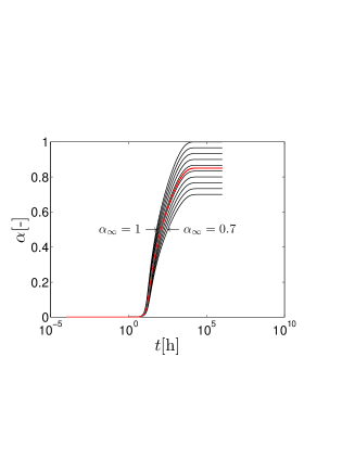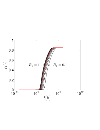
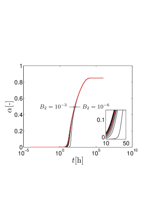
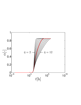
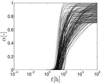
The affinity hydration model was chosen not only for its nonlinearity, but especially for its relatively simple interpretation and computationally fast simulation. Hence, we assume that the model is eligible to illustrate typical features of particular identification strategies. In order to understand the influence of the model parameters to its response more deeply, Figure 3 demonstrates the changes of the response induced by changes in a chosen parameter while other parameters are fixed. On the other hand, to illustrate the spread of the model response corresponding to the parameters varying within the given domain, we prepare a design of experiments (DoE) having $N_{\mathrm{DoE}}=100$ samples in the space of standardised parameters. The DoE is generated as Latin Hypercube Sampling optimised with respect to the modified $L_{2}$ discrepancy. Such an experimental design has a good space-filling property and is nearly orthogonal [38]. For each design point we perform a model simulation to obtain a bundle of $N_{\mathrm{DoE}}$ curves for the degree of hydration $\alpha(t)$, see Figure 4a.

(a)	(b)

Figure 4: Bundle of degree of hydration curves obtained for design points (a) and sensitivity analysis for input-output pairs (b).

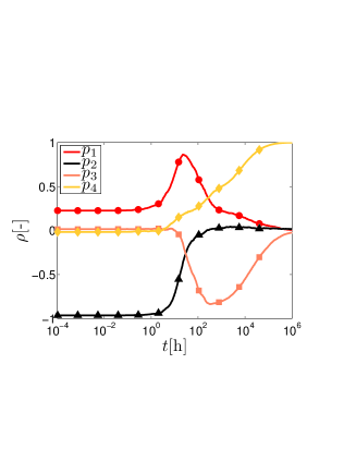
Since the model response is represented by the degree of hydration being a function of the time, the time domain is discretised into $1161$ steps uniformly distributed with the logarithm of the time. Hence, the model input vector $\mathchoice{\displaystyle\boldsymbol{p}}{\textstyle\boldsymbol{p}}{\scriptstyle\boldsymbol{p}}{\scriptscriptstyle\boldsymbol{p}}=(p_{1},p_{2},p_{3},p_{4})$ consists of $4$ parameters and the output vector $\mathchoice{\displaystyle\boldsymbol{\alpha}}{\textstyle\boldsymbol{\alpha}}{\scriptstyle\boldsymbol{\alpha}}{\scriptscriptstyle\boldsymbol{\alpha}}=(\alpha_{1},\dots,\alpha_{N_{\mathrm{time}}})$ consists of $N_{\mathrm{time}}=1161$ components. In order to quantify the influence of the model parameters to particular response components, we evaluate Spearman’s rank correlation coefficient $\rho$ for each $(\mathchoice{\displaystyle\boldsymbol{p}}{\textstyle\boldsymbol{p}}{\scriptstyle\boldsymbol{p}}{\scriptscriptstyle\boldsymbol{p}}_{i},\mathchoice{\displaystyle\boldsymbol{\alpha}}{\textstyle\boldsymbol{\alpha}}{\scriptstyle\boldsymbol{\alpha}}{\scriptscriptstyle\boldsymbol{\alpha}}_{i})$ pair using all the $i\in\{1,\dots,N_{\mathrm{DoE}}\}$ simulations. The results of such a sampling-based sensitivity analysis [36] are plotted in Figure 4b.

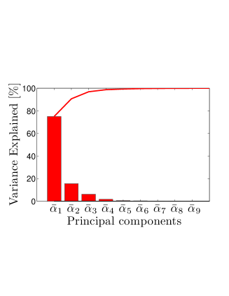
In the inverse mode of identification, the model output vector $\mathchoice{\displaystyle\boldsymbol{\alpha}}{\textstyle\boldsymbol{\alpha}}{\scriptstyle\boldsymbol{\alpha}}{\scriptscriptstyle\boldsymbol{\alpha}}$ consisting of $N_{\mathrm{time}}=1161$ components is too large for usage as an input vector for the ANN. Hence, we performed the principal component analysis (PCA) in order to reduce this number to $N_{\mathrm{PCA}}=100$ components $\bar{\mathchoice{\displaystyle\boldsymbol{\alpha}}{\textstyle\boldsymbol{\alpha}}{\scriptstyle\boldsymbol{\alpha}}{\scriptscriptstyle\boldsymbol{\alpha}}}=(\bar{\alpha}_{1},\dots,\bar{\alpha}_{2})$ with non-zero variance (this number is related to the number of simulations involved in PCA, i.e. $N_{\mathrm{PCA}}=N_{\mathrm{DoE}}$). The components are ordered according to their relative variance, see Figure 5a for the nine most important ones.

(a)	(b)

Figure 5: Variance explained by the first nine principal components (a) and sensitivity analysis for model inputs $\mathchoice{\displaystyle\boldsymbol{p}}{\textstyle\boldsymbol{p}}{\scriptstyle\boldsymbol{p}}{\scriptscriptstyle\boldsymbol{p}}_{i}$ - principal components $\bar{\mathchoice{\displaystyle\boldsymbol{\alpha}}{\textstyle\boldsymbol{\alpha}}{\scriptstyle\boldsymbol{\alpha}}{\scriptscriptstyle\boldsymbol{\alpha}}}_{i}$ (b).

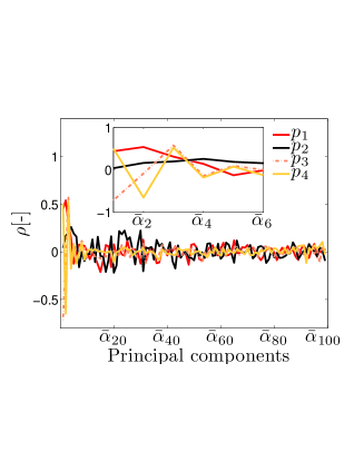
Resulting principal components are technically new quantities obtained by a linear combination of the original model outputs $\bar{\mathchoice{\displaystyle\boldsymbol{\alpha}}{\textstyle\boldsymbol{\alpha}}{\scriptstyle\boldsymbol{\alpha}}{\scriptscriptstyle\boldsymbol{\alpha}}}=\bar{A}(\mathchoice{\displaystyle\boldsymbol{\alpha}}{\textstyle\boldsymbol{\alpha}}{\scriptstyle\boldsymbol{\alpha}}{\scriptscriptstyle\boldsymbol{\alpha}})$. This transformation has of course an influence to sensitivity analysis and thus we computed correlations between the model inputs $\mathchoice{\displaystyle\boldsymbol{p}}{\textstyle\boldsymbol{p}}{\scriptstyle\boldsymbol{p}}{\scriptscriptstyle\boldsymbol{p}}_{i}$ and principal components $\bar{\mathchoice{\displaystyle\boldsymbol{\alpha}}{\textstyle\boldsymbol{\alpha}}{\scriptstyle\boldsymbol{\alpha}}{\scriptscriptstyle\boldsymbol{\alpha}}}_{i}$, see Figure 5b.

6 Implementation of approximation strategies

Results of the described simulations are also used as training simulations for ANNs, i.e. $\mathcal{D}_{\mathrm{train}}=\{(\mathchoice{\displaystyle\boldsymbol{p}}{\textstyle\boldsymbol{p}}{\scriptstyle\boldsymbol{p}}{\scriptscriptstyle\boldsymbol{p}}_{i},\mathchoice{\displaystyle\boldsymbol{\alpha}}{\textstyle\boldsymbol{\alpha}}{\scriptstyle\boldsymbol{\alpha}}{\scriptscriptstyle\boldsymbol{\alpha}}_{i})\,|\,i\in\{1,2,\dots,N_{\mathrm{train}}\},N_{\mathrm{train}}=N_{\mathrm{DoE}}=100\}$. Particular approximation strategies, however, process the training simulations in a different way.

The strategy of the forward model approximation can be formulated in two ways, which differ in handling the high dimensionality of the model output $\mathchoice{\displaystyle\boldsymbol{\alpha}}{\textstyle\boldsymbol{\alpha}}{\scriptstyle\boldsymbol{\alpha}}{\scriptscriptstyle\boldsymbol{\alpha}}$. In the first formulation, we can consider the time step $t_{k}$ as the fifth model parameter (i.e. the fifth model input) and thus the model output reduces into only one scalar value of the hydration degree $\alpha_{k}$ corresponding to the given time $t_{k}$. As the objective of the ANN is thus to span the parameter as well as the time space, we called this strategy as Forward Complex (ForwComp). In such a configuration, the results of $N_{\mathrm{train}}$ training simulations turn into $N_{\mathrm{train}}\times N_{\mathrm{time}}=116,100$ training samples. Evaluation of so many samples at every iteration of the ANN’s training process is, however, very time-consuming. Therefore, only every $m$-th time step is included for ANN training and thus the training set is given as $\mathcal{D}_{\mathrm{train}}^{\mathrm{ForwComp}}=\{((\mathchoice{\displaystyle\boldsymbol{p}}{\textstyle\boldsymbol{p}}{\scriptstyle\boldsymbol{p}}{\scriptscriptstyle\boldsymbol{p}}_{i},t_{k}),\alpha_{i,k})\,|\,i\in\{1,2,\dots,N_{\mathrm{train}}\},k\in\{1,1+m,1+2m,\dots,N_{\mathrm{time}}\}\}$. In our particular implementation, we selected $m=10$ leading to $|\mathcal{D}_{\mathrm{train}}^{\mathrm{ForwComp}}|=11,700$ samples. Note that in all other strategies, the number of training samples equals the number of training simulations, see Table 2, where the significant parameters of particular approximation strategies are briefly summarised.

Strategy	$N_{\mathrm{ANN}}$	Inputs	Outputs	$|\mathcal{D}_{\mathrm{train}}|$
Forward Complex	$1$	$p_{1}$, $p_{2}$, $p_{3}$, $p_{4}$, $t_{k}$	$\alpha_{k}\,|\,k\in\{1,11,\dots,1161\}$	$11700$
Forward Split	$9$	$p_{1}$, $p_{2}$, $p_{3}$, $p_{4}$	$\alpha_{300};\alpha_{400};\dots;\alpha_{1100}$	$100$
Forward Split II	$22$	$p_{1}$, $p_{2}$, $p_{3}$, $p_{4}$	$\alpha_{100};\alpha_{150};\dots;\alpha_{1150}$	$100$
Forward Split III	$43$	$p_{1}$, $p_{2}$, $p_{3}$, $p_{4}$	$\alpha_{100};\alpha_{130};\alpha_{150};\alpha_{170};\dots;\alpha_{1150}$	$100$
Error $F_{1}$	$1$	$p_{1}$, $p_{2}$, $p_{3}$, $p_{4}$	$F_{1}$	$100$
Error $F_{2}$	$1$	$p_{1}$, $p_{2}$, $p_{3}$, $p_{4}$	$F_{2}$	$100$
Inverse Expert	$4$	$\alpha_{300},\alpha_{400},\dots,\alpha_{1100}$	$p_{1}$; $p_{2}$; $p_{3}$; $p_{4}$	$100$
Inverse Expert II	$4$	$\alpha_{200},\alpha_{300},\dots,\alpha_{1100}$	$p_{1}$; $p_{2}$; $p_{3}$; $p_{4}$	$100$
Inverse PCA	$4$	$\bar{\alpha}_{1},\bar{\alpha}_{2},\dots,\bar{\alpha}_{9}$	$p_{1}$; $p_{2}$; $p_{3}$; $p_{4}$	$100$

Table 2: Parameters of approximation strategies

The second way of the model output approximation is based on training an independent ANN for every time step $t_{k}$. Here, the particular ANN approximates simpler relation and span only the parameter space. A training data set for ANN approximating the response component $\alpha_{k}$ is thus given as $\mathcal{D}_{\mathrm{train}}^{\mathrm{ForwSpli,}\alpha_{k}}=\{(\mathchoice{\displaystyle\boldsymbol{p}}{\textstyle\boldsymbol{p}}{\scriptstyle\boldsymbol{p}}{\scriptscriptstyle\boldsymbol{p}}_{i},\alpha_{i,k})\,|\,i\in\{1,2,\dots,100\}\}$ having only $|\mathcal{D}_{\mathrm{train}}^{\mathrm{ForwSpli,}\alpha_{k}}|=100$ samples. A disadvantage of such an approach consists in training a large number $N_{\mathrm{ANN}}$ of smaller ANNs. As training of $N_{\mathrm{ANN}}=N_{\mathrm{time}}=1161$ different ANNs can be almost unfeasible, we select only a few of the time steps, where the approximation is constructed and thus, the model output approximation is more rough. The choice of the important time steps and their number can be driven by the expert knowledge or results of the sensitivity analysis. Hence, we present three different choices so as to illustrate its influence, see Table 2. We further call these strategies as Forward Split (ForwSpli), Forward Split II (ForwSpliII) and Forward Split III (ForwSpliIII).

The error function approximation is the only strategy where the high dimensionality of the model output does not impose any complications. The model output is used for evaluation of the error function and the ANN is trained to approximate the mapping from the parameter space to a single scalar value of the error function, i.e. $\mathcal{D}_{\mathrm{train}}^{\mathrm{Error,}F_{a}}=\{(\mathchoice{\displaystyle\boldsymbol{p}}{\textstyle\boldsymbol{p}}{\scriptstyle\boldsymbol{p}}{\scriptscriptstyle\boldsymbol{p}}_{i},F_{a})\,|\,i\in\{1,2,\dots,N_{\mathrm{train}}\}\}$ and $|\mathcal{D}_{\mathrm{train}}^{\mathrm{Error,}F_{a}}|=100$, where $F_{a}$ stands for a chosen error function. As we already mentioned in Section 3, there are two very common error functions given by Eqs. (3) and (4) and thus we investigate both considering the two strategies further called as Error $F_{1}$ and Error $F_{2}$, respectively.

In case of the inverse relation approximation, the high dimensionality of the model output needs again some special treatment so as to keep the number of ANN inputs and thus the ANN complexity reasonable. An intuitive approach is a simple selection of a limited number of output values $\mathchoice{\displaystyle\boldsymbol{a}}{\textstyle\boldsymbol{a}}{\scriptstyle\boldsymbol{a}}{\scriptscriptstyle\boldsymbol{a}}=A(\mathchoice{\displaystyle\boldsymbol{\alpha}}{\textstyle\boldsymbol{\alpha}}{\scriptstyle\boldsymbol{\alpha}}{\scriptscriptstyle\boldsymbol{\alpha}})$. Here, one ANN is trained to predict one model parameter $p_{j}$ and thus $\mathcal{D}_{\mathrm{train}}^{\mathrm{InvExp},p_{j}}=\{(\mathchoice{\displaystyle\boldsymbol{a}}{\textstyle\boldsymbol{a}}{\scriptstyle\boldsymbol{a}}{\scriptscriptstyle\boldsymbol{a}}_{i},p_{i,j})\,|\,i\in\{1,2,\dots,N_{\mathrm{train}}\}\}$ and $|\mathcal{D}_{\mathrm{train}}^{\mathrm{InvExp,}p_{j}}|=100$. A particular choice of components in the vector $\mathchoice{\displaystyle\boldsymbol{a}}{\textstyle\boldsymbol{a}}{\scriptstyle\boldsymbol{a}}{\scriptscriptstyle\boldsymbol{a}}_{i}$ defined by the operator $A$ should take into account not only the results of sensitivity analysis, but also a possible measurement error in experimental data as well as any other expert knowledge. Hence we present again two different choices in order to illustrate its influence, see Table 2 and we further call these configurations as Inverse Expert (InvExp) and Inverse Expert II (InvExpII).

In order to reduce the influence of the expert choice, the principal components $\bar{\mathchoice{\displaystyle\boldsymbol{\alpha}}{\textstyle\boldsymbol{\alpha}}{\scriptstyle\boldsymbol{\alpha}}{\scriptscriptstyle\boldsymbol{\alpha}}}$ computed as described in the previous section can be used as the ANN’s inputs and one has to choose only their number. To compare the information contained in the same number of inputs selected by an expert, we have chosen the same number of principal components as the number of inputs in the Inverse Expert configuration and thus $\mathcal{D}_{\mathrm{train}}^{\mathrm{InvPCA},p_{j}}=\{((\bar{\alpha}_{i,1},\dots,\bar{\alpha}_{i,9}),p_{i,j})\,|\,i\in\{1,2,\dots,N_{\mathrm{train}}\}\}$ and $|\mathcal{D}_{\mathrm{train}}^{\mathrm{InvPCA,}p_{j}}|=100$. The principal components based strategy is further called Inverse PCA (InvPCA). In our preliminary study presented in [10], we have also tested the possibility to choose smaller number of PCA-based inputs selected separately for each parameter to be identified according to the sensitivity analysis. Nevertheless, such sensitivity-driven reduction of PCA-based inputs was shown to deteriorate the quality of trained ANNs.

Then, the last preparatory step concerns the generation of testing data for a final assessment of the resulting ANNs consisting of $N_{\mathrm{test}}=50$ simulations for randomly generated sets of input parameters. The obtained data are then processed by particular approximation strategies in the same way as the training data described above.

7 Neural network training algorithm and topology choice

The quality of the ANN-based approximation estimated on a given data set $\mathcal{D}$ can be expressed as the mean relative prediction error $\varepsilon^{\mathrm{MRP}}(\mathcal{D})$ given as

$$\varepsilon^{\mathrm{MRP}}(\mathcal{D})=\frac{\sum^{|\mathcal{D}|}_{i=1}|O_{i}-T_{i,\mathcal{D}}|}{|\mathcal{D}|(T_{\mathrm{max,\mathcal{D}_{train}}}-T_{\mathrm{min,\mathcal{D}_{train}}})}\,,$$ (10)

where $O_{i}$ is the ANN’s output corresponding to the target value $T_{i,\mathcal{D}}$ contained in the data set $\mathcal{D}$, which consists of $|\mathcal{D}|$ samples. $T_{\mathrm{max,\mathcal{D}_{train}}}$ and $T_{\mathrm{min,\mathcal{D}_{train}}}$ are the maximal and minimal target values in the training data set $\mathcal{D}_{\mathrm{train}}$, so the error $\varepsilon^{\mathrm{MRP}}(\mathcal{D})$ is always scaled by the same factor for any chosen data set $\mathcal{D}$ and this factor corresponds to the range of the training data.

The conjugate gradient-based method [39] was applied as a training algorithm for synaptic weights computation and the cross-validation method was employed to determine the number of hidden neurons. In $V$-fold cross-validation we break the training data set $\mathcal{D}_{\mathrm{train}}$ into $V$ approximately equisized subsets $\mathcal{D}_{\mathrm{train}}=\mathcal{D}_{\mathrm{train},1}\cup\mathcal{D}_{\mathrm{train},2}\cup\dots\cup\mathcal{D}_{\mathrm{train,}V}$ and then we perform $V$ training processes, each time leaving out one of the subsets $\mathcal{D}_{\mathrm{train},i}$ and using the rest of the training data set $\mathcal{D}_{\mathrm{train}}\setminus\mathcal{D}_{\mathrm{train,i}}$.

The criterion for stopping the training process is governed by the prediction errors ratio $r^{\mathrm{PE}}_{k}$ computed at the $k$-th iteration of the training algorithm given as

$$r^{\mathrm{PE}}_{k}(\mathcal{D}_{\mathrm{train}}\setminus\mathcal{D}_{\mathrm{train,i}})=\frac{\sum_{j=k-J}^{k}\varepsilon^{\mathrm{MRP}}_{j}(\mathcal{D}_{\mathrm{train}}\setminus\mathcal{D}_{\mathrm{train,i}})}{\sum_{j=k-2J}^{k-J-1}\varepsilon^{\mathrm{MRP}}_{j}(\mathcal{D}_{\mathrm{train}}\setminus\mathcal{D}_{\mathrm{train,i}})}\,,$$ (11)

where $\varepsilon^{\mathrm{MRP}}_{j}(\mathcal{D}_{\mathrm{train}}\setminus\mathcal{D}_{\mathrm{train,i}})$ is the mean relative prediction error obtained at the $j$-th iteration of the training algorithm obtained on the training data set without its $i$-th partition. $J$ is the chosen number of iterations considered for computing the ratio $r^{\mathrm{PE}}_{k}$ for its smoothing effect on $r^{\mathrm{PE}}_{k}$. The training process is stopped either when the number of iterations achieves its chosen maximal value $K$ or if the prediction errors ratio $r^{\mathrm{PE}}_{k}$ exceeds a chosen critical value $r^{\mathrm{PE}}_{\mathrm{max}}$.

Once the training process is completed, the ANN is evaluated on the remaining part of the training data $\mathcal{D}_{\mathrm{train,i}}$, which was not used in the training process. The quality of the ANN with a particular number of hidden neurons $h$ is assessed by the cross-validation error $\varepsilon^{\mathrm{CV}}_{h}$, which is computed as a mean of the errors obtained for the ANNs trained on the subsets $\mathcal{D}_{\mathrm{train}}\setminus\mathcal{D}_{\mathrm{train,i}}$ and then evaluated on the remaining subset $\mathcal{D}_{\mathrm{train,i}}$ , i.e.

$$\varepsilon^{\mathrm{CV}}_{h}=\frac{1}{V}\sum_{i=1}^{V}\varepsilon^{\mathrm{MRP}}(\mathcal{D}_{\mathrm{train,i}})\,.$$ (12)

We start with an ANN having $h_{\mathrm{min}}$ hidden neurons and we compute the corresponding cross-validation error. Then, one hidden neuron is added and after all the training processes on training data subsets, the new cross-validation error is evaluated. We compute the cross-validation error ratio $r^{\mathrm{CVE}}_{h}$ as

$$r^{\mathrm{CVE}}_{h}=\varepsilon^{\mathrm{CV}}_{h}/\varepsilon^{\mathrm{CV}}_{h-1}\,.$$ (13)

We count the situations when the ratio $r^{\mathrm{CVE}}_{h}$ exceeds a chosen critical value $r^{\mathrm{CVE}}_{\mathrm{max}}$. If this happened $W$ times, the addition of hidden neurons is stopped. Then we choose the architecture having the smallest cross-validation error $\varepsilon^{\mathrm{CV}}_{h}$ and the particular ANN with the synaptic weights having the smallest training error $\varepsilon^{\mathrm{MRP}}$.

Number of subsets in cross-validation	$V$	$10$
Number of iteration considered in $r^{\mathrm{PE}}_{k}$	$J$	100
Maximal number of training iterations	$K$	$5000$
Maximal value of prediction errors ratio	$r^{\mathrm{PE}}_{\mathrm{max}}$	$0.999$
Starting value of hidden neurons	$h_{\mathrm{min}}$	$1$
Maximal value of cross-validation error ratio	$r^{\mathrm{CVE}}_{\mathrm{max}}$	$0.99$
Maximal value of $r^{\mathrm{CVE}}_{\mathrm{max}}$ exceeding	$W$	$3$

Table 3: Parameters of ANN training algorithm and cross-validation method

The resulting ANNs are tested on an independent testing data set $\mathcal{D}_{\mathrm{test}}$. Since some of the approximation strategies consist of a high number of ANNs, the resulting number of hidden neurons and achieved errors on training and testing data for all the trained ANNs are listed in A. Brief summary of these results is presented in Table 4.

Strategy	$h$	$\varepsilon^{\mathrm{MRP}}(\mathcal{D}_{\mathrm{train}})[\%]$	$\varepsilon^{\mathrm{MRP}}(\mathcal{D}_{\mathrm{test}})[\%]$
Forward Complex	$7$	$2.03$	$2.67$
Forward Split	$3$ to $10$	$0.06$ to   $1.06$	$0.06$ to   $1.27$
Forward Split II	$4$ to $13$	$0.06$ to   $1.42$	$0.07$ to   $2.04$
Forward Split III	$3$ to $13$	$0.03$ to   $1.50$	$0.03$ to   $1.98$
Error $F_{1}$	$10$	$0.40$ to   $0.54$	$0.57$ to   $0.74$
Error $F_{2}$	$9$ to $11$	$0.78$ to   $1.36$	$0.96$ to   $1.56$
Inverse Expert	$5$ to   $8$	$1.14$ to   $5.74$	$1.31$ to   $6.43$
Inverse Expert II	$4$ to   $6$	$1.38$ to   $5.79$	$1.36$ to   $6.52$
Inverse PCA	$4$ to   $8$	$0.28$ to $10.50$	$0.33$ to $16.73$

Table 4: Architecture of particular ANNs in inverse strategies and their errors on training and testing data.

Regarding the number of hidden neurons, the results point to higher complexity of the error function relationships. Nevertheless, the differences in hidden neurons among particular strategies are relatively small.

The quality of the resulting ANNs in approximation of the given relationships is measured by the obtained errors on all the training $\varepsilon^{\mathrm{MRP}}(\mathcal{D}_{\mathrm{train}})$ and testing $\varepsilon^{\mathrm{MRP}}(\mathcal{D}_{\mathrm{test}})$ data. Small differences between the training and testing errors refer to well-trained ANNs and to the good quality of the training method as well as the method for topology estimation. Note that overtrained ANNs usually lead to significantly higher errors on testing data.

Comparing the approximation quality of the particular strategies, we can point out good results of the forward model approximation and error function approximation, where the errors did not exceed the value of $3$ %. The good approximation of the forward model is not surprising since the relationship is well-defined, smooth and relatively simple. The good results of the error function approximation are more unexpected, because the relationship here is probably more nonlinear and complex. One possible explanation is a large spread of error function values on the training data, which is used to scale the errors (see Eq. (10)). While the error functions converge to zero near the optimal parameter values, they quickly rise to extremely high values for parameter values more distant from the optimum. Hence, we presume that the small errors obtained in the error function approximation do not promise comparably good results in the final parameter identification.

The results of the inverse relation approximation are not very good, but it was foreseen due to unknown and probably ill-posed relationship. Nevertheless, the obtained errors are actually the final errors of the whole identification process for the training and testing data, since there is no other following step concerning any optimisation as in the case of other identification strategies. Hence, further comments on these results are presented in the following section concerning verification of the overall identification strategies on the testing data.

8 Verification of model calibration

Since the errors in Table 4 represent only the quality of the constructed ANNs, we have to also investigate the quality of the identification procedures. This section is devoted to verification of the model calibration, where the goal is to predict the model parameters’ values corresponding to the simulated data, which are not perturbated by any noise. The advantage of verification is that we also know the true values of the parameters and thus, we can easily evaluate the quality of their estimation by each strategy. In particular, the calibration strategies were applied to estimate the parameters’ values for all the training and testing simulations.

As mentioned, in case of the inverse relation approximation, the outputs of ANNs are directly the predicted values of the identified parameters $\widehat{\mathchoice{\displaystyle\boldsymbol{p}}{\textstyle\boldsymbol{p}}{\scriptstyle\boldsymbol{p}}{\scriptscriptstyle\boldsymbol{p}}}$. In case of the forward model approximation, we have to run a subsequent optimisation process. Here, the evolutionary algorithm GRADE, see [9] for details about this method, is applied to find a set of parameters’ values $\widehat{\mathchoice{\displaystyle\boldsymbol{p}}{\textstyle\boldsymbol{p}}{\scriptstyle\boldsymbol{p}}{\scriptscriptstyle\boldsymbol{p}}}$ minimising the square distance $\delta$ between components of the model response $\alpha_{k}$ and their corresponding ANN-based approximated counterparts $\widetilde{\alpha}_{k}$, i.e.

$$\delta=\sum_{k}(\alpha_{k}-\widetilde{\alpha}_{k})^{2}\,,$$ (14)

where $k$ corresponds to the selected approximated components defined for particular identification strategies in Table 2. In such a way, the parameters $\widehat{\mathchoice{\displaystyle\boldsymbol{p}}{\textstyle\boldsymbol{p}}{\scriptstyle\boldsymbol{p}}{\scriptscriptstyle\boldsymbol{p}}}$ are predicted for all the training as well as testing data. As the true values of parameters $\mathchoice{\displaystyle\boldsymbol{p}}{\textstyle\boldsymbol{p}}{\scriptstyle\boldsymbol{p}}{\scriptscriptstyle\boldsymbol{p}}$ are known in the verification process, the mean prediction errors $\widehat{\varepsilon}$ are computed relatively to the spread of the training data, i.e.

$$\widehat{\epsilon}(\widehat{p}_{j})=\frac{\sum_{i=1}^{|\mathcal{D}|}|p_{i,j}-\widehat{p}_{i,j}|}{|\mathcal{D}|(p_{\mathrm{max}(\mathcal{D}_{\mathrm{train}}),j}-p_{\mathrm{min}(\mathcal{D}_{\mathrm{train}}),j})}\,,$$ (15)

and the obtained errors for particular identification strategies are listed in Table 5.

	$\widehat{\varepsilon}(\widehat{p}_{1})$		$\widehat{\varepsilon}(\widehat{p}_{2})$		$\widehat{\varepsilon}(\widehat{p}_{3})$		$\widehat{\varepsilon}(\widehat{p}_{4})$		$\widehat{\varepsilon}(\widehat{\alpha})$
	train	test	train	test	train	test	train	test	train	test
Forward Complex	16.78	17.09	52.20	47.91	6.06	5.45	3.67	2.69	1.079	1.088
Forward Split	9.48	11.62	30.18	38.45	3.14	4.65	1.17	3.10	0.310	0.370
Forward Split II	5.09	6.47	13.34	15.03	1.69	2.60	0.67	1.02	0.144	0.205
Forward Split III	4.12	4.84	10.73	10.65	1.49	1.63	0.57	0.64	0.124	0.160
Inverse Expert	5.74	6.43	5.15	6.21	1.99	2.16	1.14	1.31	0.490	0.493
Inverse Expert II	5.79	6.23	5.60	6.52	2.60	3.18	1.38	1.36	0.444	0.533
Inverse PCA	3.86	5.10	10.50	16.73	1.25	1.89	0.28	0.33	0.377	1.209

Table 5: Results of verification of particular identification strategies in terms of mean relative prediction errors $\widehat{\varepsilon}$ [%]. Best results are highlighted in bold font.

In application of the identification strategy to real experimental data, the parameter values are not known, but the success of the identification process is quantified by quality of fitting the data by the model response obtained for the identified parameters. Hence, the model simulations were performed for all the identified parameter sets and prediction errors $\widetilde{\varepsilon}$ in terms of predicted responses $\widetilde{\mathchoice{\displaystyle\boldsymbol{\alpha}}{\textstyle\boldsymbol{\alpha}}{\scriptstyle\boldsymbol{\alpha}}{\scriptscriptstyle\boldsymbol{\alpha}}}$ are computed analogously to the Eq. (15). Their values averaged also over all the response components are then listed in Table 5.

The results for the strategies based on an approximation of the error function are missing here, because they require to build a particular ANN for every curve of the hydration degree and for each require to run an additional minimisation procedure. This is overwhelming and thus these strategies are only validated on the experimental data as described in the following section.

One can see that among the forward strategies, the complex variant provided the worst results in the training process as well as in the final identification. The complex relationship covering the time domain causes apparently certain difficulties to the training process. We can conclude that training of a set of neural networks means more work, but offers significantly better quality of the model approximation. We can also point out the large differences in errors of particular parameters, which correspond to influence of particular parameters to the model response. As demonstrated in Figure 3, the largest spread of the model response is related namely to change in the parameters $p_{4}$ and $p_{3}$, while the parameter $p_{1}$ and also $p_{2}$ seem to be almost negligible. The sensitivity analysis illustrated in Figure 4b shows very high sensitivity of the model response to the parameter $p_{2}$ at early stage of hydration, nevertheless, at this stage the spread of the model response is almost negligible and even a very small error in the response approximation can be fatal for identification of the parameter $p_{2}$. On the other hand, it is not surprising that the identification accuracy is significantly improved with an increasing number of approximated response components, i.e. an increasing number of trained ANNs.

Despite the worse results in training of ANNs, the inverse strategies achieved comparably good results with the forward strategies in parameter identification and also in fitted measurements. More precisely, the results of measurements fitting are slightly worse, but the errors in parameter prediction are smaller. Especially the Inverse Expert strategies provided surprisingly small errors in $p_{2}$ prediction and the errors in parameters are generally more balanced. This phenomenon can be possibly explained by fact that each ANN is trained to predict each parameter separately, thus automatically selecting and emphasizing the combinations of the model response critical for the parameter. In the strategy Inverse Expert II, the usage of one additional input at the early stage of hydration caused no improvement of the resulting prediction, which is probably caused again by fact that the responses at this stage have a negligible spread and almost no predictive value. The last interesting result concerns the application of principal component analysis. The Inverse PCA strategy provided again significantly different errors in prediction of particular parameters, similarly to the forward strategies. The reason resides possibly in fact that PCA emphasize the most important components, while it can mix the effects of the less significant parameters. Nevertheless, when compared with strategies Forward Split and Inverse Expert using the same number of response components, the Inverse PCA provided the best results in prediction of all the parameters except $p_{2}$. Its quality of measurement fitting is, however, the worst among those strategies.

From this thorough comparison we may conclude that all the inverse strategies provide very good results, which makes them highly promising considering their very simple implementation which does not include any additional optimisation process except the only training of ANNs. Moreover, the Inverse Expert strategies can be especially recommended for identification of less significant parameters.

9 Validation of model calibration

The previous section was focused on mutual comparison of the presented identification strategies on simulated data. However, a complete comparison has to include their validation on experimental data. To that purpose we used the four experimental data obtained by isothermal calorimetry: one for cement “Mokra” CEM I 42.5 R taken directly from Heidelberg cement group’s kiln in Mokrá, Czech Republic [35] and three others from the following literature: “Boumiz” [40], “Hua” [41] and “Princigallo” [42].

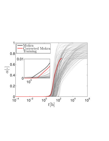
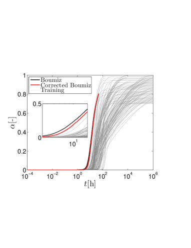
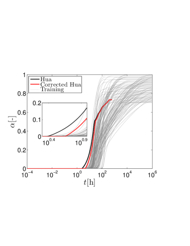
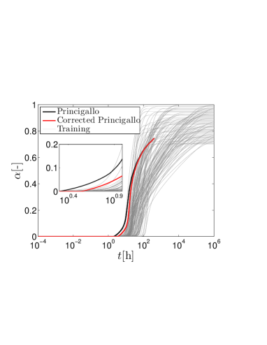
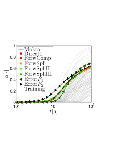
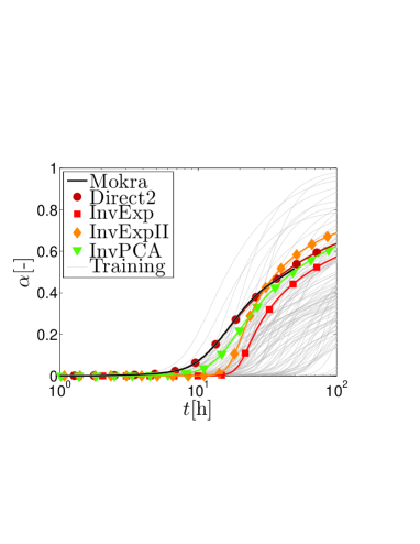
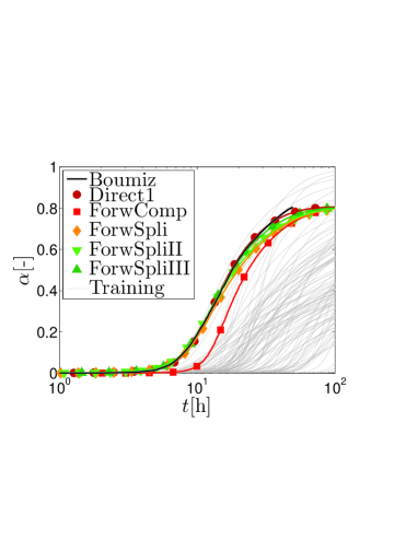
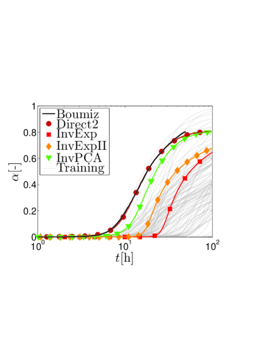
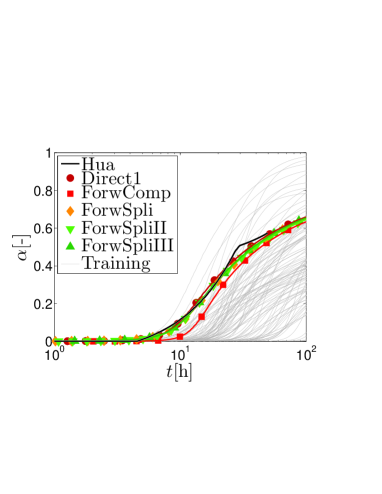
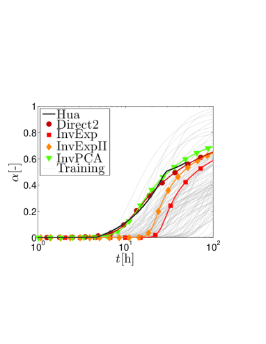
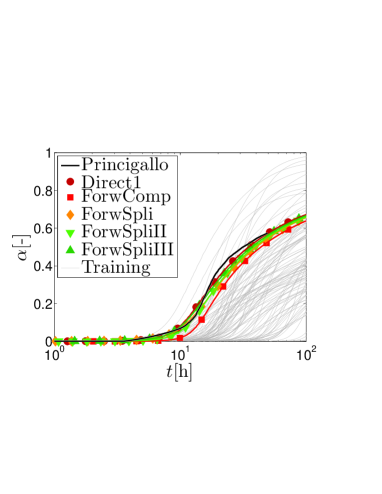
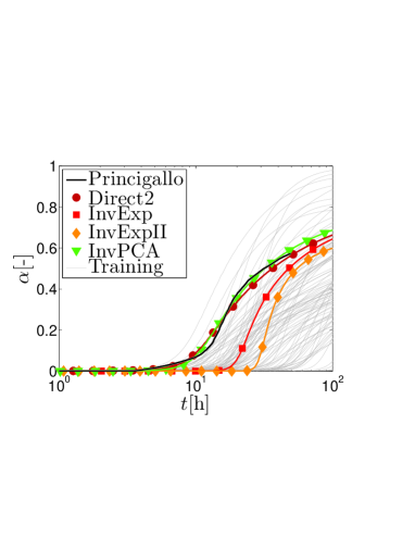
In parameter identification from experimental data, one often face to difficulties related to (i) experimental errors and (ii) model imperfections. Especially in case of models with parameters having a specific physical meaning – like the affinity hydration model – it happens that the experimental data seems to lie beyond the physically meaningful values of the model parameters. This is exactly what we face in case of the four experimental curves depicted in Figure 6.

correction: $0.5$ h	correction: $1$ h
correction: $4.5$ h	correction: $3.5$ h

Figure 6: Corrections of experimental curves.

The grey curves represent the training samples generated in an optimised fashion so as to maximally cover the parameter space. Nevertheless, it is visible that all the experimental curves lie out of the bundle of the training samples. Applying the identification strategies to these data will require the ANNs to extrapolate and it will probably lead to unphysical and wrong predictions of the model parameters. Such results were presented for “Mokra” in [11]. Looking in more detail on the experimental curves, one can see that the difference between the experimental data and simulations can be explained by wrong estimation of the origin of hydration. Correction of the starting time moves the curves into the bundle of response simulations. As a matter of fact, the correction in orders of hours is negligible comparing to the duration of the whole hydration process lasting often days or weeks. Moreover, the goal of this paper is not to argue against the correctness of the model or data, but to demonstrate the properties of particular identification strategies which can be better illustrated in a situation, where the observed data are not outliers w.r.t. sampled parameter domain. For an interested reader about the identification of outliers we refer to [11].

In general, validation does not allow for a comparison in terms of parameters’ values, because these are not known a priori. Nevertheless, the simplicity and the fast simulation of the affinity hydration model permit a direct optimisation of the model parameters so as to fit the measured data without any incorporated approximation. The resulting optimal solutions can be then compared with the results obtained using the ANN approximations. To that purpose, we employ again the error functions given in Eqs. (3) and (4) and the GRADE algorithm with the same setting as in the previous section to minimise the both error functions. The obtained results are referred to as Direct1 and Direct2, respectively, and they represent the best results that can be achieved with the current model on the given data.

Subsequently, the identification strategies were applied to the experimental data using the prepared ANNs. Since the ANNs are constructed for specific time steps of the hydration degree, the experimental curves are interpolated to the time steps required by the particular ANNs. If necessary, the data are extrapolated beyond the last measured time step assuming the further progress of hydration to be constant at the last measured value. The identified parameters together with the parameters’ values obtained by the direct optimisation are written in Tables 6 and 7. Note that the parameter values highlighted in bold font refer to situation, where the measured data lie beyond the domain of training data and the ANN is forced to extrapolate.

	“Mokra”					“Boumiz”
Method	$p_{1}$	$p_{2}$	$p_{3}$	$p_{4}$	$\widehat{\varepsilon}(\widehat{\alpha})$	$p_{1}$	$p_{2}$	$p_{3}$	$p_{4}$	$\widehat{\varepsilon}(\widehat{\alpha})$
Direct1	0.84	0.99	0.18	0.05	0.70	0.93	1.00	0.02	0.36	2.37
Direct2	0.82	0.98	0.18	0.05	0.65	0.93	1.00	0.02	0.35	2.70
Forward Complex	0.81	1.00	0.18	0.03	1.35	1.00	0.61	0.08	0.36	12.67
Forward Split	0.82	1.00	0.19	0.05	1.15	0.96	1.00	0.08	0.35	5.44
Forward Split II	0.78	1.01	0.18	0.05	0.83	1.00	1.00	0.08	0.35	4.11
Forward Split III	0.80	1.00	0.19	0.05	0.91	0.98	1.00	0.05	0.35	3.03
Error $F_{1}$	0.78	0.73	0.09	0.07	3.89	-	-	-	-	-
Error $F_{2}$	1.00	1.19	0.15	-0.06	2.73	-	-	-	-	-
Inverse Expert	1.16	-0.18	0.29	0.03	6.83	0.78	-0.24	0.22	0.30	35.11
Inverse Expert II	1.21	-0.06	0.19	0.16	4.68	1.27	-0.14	0.20	0.13	25.94
Inverse PCA	0.75	0.83	0.18	0.06	1.82	0.78	0.87	0.02	0.35	10.82

Table 6: Results of identification strategies obtained for “Mokra” and “Boumiz”: identified values of model parameters and mean relative error in degree of hydration $\widehat{\varepsilon}(\widehat{\alpha})$ [%].

	“Hua”					“Princigallo”
Method	$p_{1}$	$p_{2}$	$p_{3}$	$p_{4}$	$\widehat{\varepsilon}(\widehat{\alpha})$	$p_{1}$	$p_{2}$	$p_{3}$	$p_{4}$	$\widehat{\varepsilon}(\widehat{\alpha})$
Direct1	1.00	0.94	0.20	0.11	2.24	1.00	0.85	0.19	0.14	3.46
Direct2	0.99	0.96	0.21	0.11	2.46	1.00	0.88	0.21	0.15	3.27
Forward Complex	1.00	0.64	0.22	0.08	4.10	1.00	0.58	0.23	0.14	6.21
Forward Split	0.87	1.00	0.19	0.11	2.84	0.78	0.98	0.18	0.15	4.39
Forward Split II	0.93	0.96	0.21	0.11	2.92	0.92	0.82	0.20	0.14	4.44
Forward Split III	0.87	1.01	0.18	0.10	2.71	0.89	0.92	0.18	0.14	3.75
Inverse Expert	0.94	-0.29	0.26	0.12	10.64	1.07	-0.16	0.22	0.15	9.02
Inverse Expert II	1.26	-0.27	0.19	0.02	6.23	1.52	-1.38	0.13	-0.24	15.05
Inverse PCA	1.00	0.89	0.15	0.12	2.41	1.13	0.74	0.19	0.15	3.62

Table 7: Results of identification strategies obtained for “Hua” and “Princigallo”: identified values of model parameters and mean relative error in degree of hydration $\widehat{\varepsilon}(\widehat{\alpha})$ [%].

The identified parameters were used as inputs for simulations, whose results are compared with the experimental data in Figures 7 and 8. To quantify the quality of obtained fits, Tables 6 and 7 contain also the mean relative error $\widehat{\varepsilon}(\widehat{\alpha})$ [%] computed in the same manner as in Table 5 for an easy comparison of the verification and validation results.

Figure 7: Comparison of corrected experimental data “Mokra” and “Boumiz” and corresponding results of calibration strategies.

Figure 8: Comparison of corrected experimental data “Hua” and “Princigallo” and corresponding results of calibration strategies.

The strategies based on the error function approximation are illustrated on the parameter identification from “Mokra” data, which are used to define the error functions, which are approximated by the ANNs. The trained ANNs are then optimised by the GRADE algorithm so as to provide the optimal set of the identified parameters. As we presumed, the identification results are not satisfactory despite very good results of the ANNs’ training processes, see Table 4. The training and testing errors are small relatively to the spread of error functions’ values, which increase quickly with the distance from the optimal solution. The strategy, however, requires high precision of the ANN’s approximation near the optimal solution, which can be hardly achieved due the overall complex shape of the error functions.

The worst results on all the experimental curves were obtained by the inverse strategies based on selected components of the model response used as the ANNs’ inputs. The results pointed out the high sensitivity of this strategy to the measurement noise and to the specific choice of the inputs. Both drawbacks are overcome by employing principal component analysis, which allows to employ a high number of the response components and filter the measurement noise out of the several first principal components. The Inverse PCA strategy thus achieved significantly better results.

The forward strategies provided generally the best results consistent with the results of verification on the simulated data. These strategies thus proved to be rather immune to the noise in experimental data.

10 Conclusions

The presented paper reviews and compares several possible applications of artificial neural networks in calibration of numerical models. In particular, the feedforward layered neural network is employed in three basic schemes to surrogate: (i) response of a model, (ii) inverse relationship of model parameters and model response and (iii) error function quantifying how well the model response fits the experimental data. Their advantages and drawbacks are illustrated on calibration of four parameters of the affinity hydration model. The model is chosen for its nonlinearity, difference in sensitivities to particular parameters on one hand and simplicity and very fast numerical evaluation on the other. The later allow for the model calibration based on the stochastic evolutionary algorithm without any involved approximation and thus better quantification of calibration results provided by the particular strategies. The investigated calibration strategies are verified on $50$ simulated curves of hydration degree and validated on four experimental ones.

Strategy	$N_{\mathrm{ANN}}$	optimisation	new data	errors
Forward Complex	$1$	yes	optimisation	middle
Forward Split	$N_{\mathrm{\alpha}}$	yes	optimisation	low
Error $F$	$1$	yes	traininng + optimisation	high
Inverse Expert	$N_{\mathrm{p}}$	no	-	high
Inverse PCA	$N_{\mathrm{p}}$	no	-	middle

Table 8: Simplified summary of calibration strategies. $N_{\mathrm{\alpha}}$ stands for a number of approximated components of model response, $N_{\mathrm{p}}$ is a number of model parameters.

Simplified summary of the obtained results is written in Table 8. One of the simplest strategies from the implementation point of view is based on an approximation of the error function (Error $F$), where only one neural network needs to be trained for the prediction of the error function values. This simplicity, however, does not hold in case of multiple experimental measurements, where the whole identification process including the neural network training as well as its optimisation needs to be done all over again for any new experiment. Moreover, the presented examples revealed that the complexity of the error function may cause difficulties for neural network training resulting in high errors in the identified parameters. The potential of the neural network is wasted on approximating the whole domain, while the accurate predictions are required only in the vicinity of the optimal values of parameters. Hence, this strategy is more suited for surrogate models based on radial basis function networks or kriging, which can be trained along with the optimisation of the error function thus allowing to improve the precision in the promising area, see e.g. [26].

An equally simple strategy is based on the approximation of the model response, where time or space variables are included among the neural network inputs (Forward Complex). This strategy is better suited for layered neural networks, which is trained only once and then can be used repeatedly for any new observations. The effort invested into the approximation of the whole domain is thus not wasted. The application to new data requires only one new optimisation process. The results obtained by this strategy were not excellent, but can be considered as satisfactory solution at a low price.

The best results were achieved by separate approximations of particular response components, where a higher number of neural networks is trained to approximate rather simple relationship defined by the calibrated model (Forward Split). This procedure requires more work on networks preparation, which is compensated by high accuracy of the obtained results. The accuracy is proportionally increasing with the number of approximated response components and can be thus influenced by work invested to the surrogate construction. Moreover, the constructed approximations can be then used again for any new data, where only the optimisation of model parameters needs to be repeated.

The worst results were obtained by the strategy approximating the inverse mapping from the response components to the model parameters (Inverse Expert). Such relationship does not have to exist and can be hardly approximated. Moreover, if the inputs for a neural network are not properly selected and thus highly sensitive to the measurement error, the procedure provides unsatisfactory results. Nevertheless, using an expert knowledge for a proper selection of inputs as presented in [28], this strategy gives good results at a very low price, since neither training nor optimisation process, but only a simple evaluation of the trained networks is needed for parameter identification from new data.

The necessity of the expert knowledge and sensitivity to the measurement error can be easily circumvented by employing principal component analysis on the model response components (Inverse PCA). Then only the number of components entering as inputs in the neural network needs to be selected. The strategy thus represents a compromise solution providing satisfactory results at a low price especially in the repeated application to new observed data.

Appendix A Configurations and results of particular neural networks

The particular choice of ANN inputs and outputs are presented in Tables 9 and 11 for forward and inverse mode strategies, respectively.

Strategy	Inputs	$h$	Output	$\varepsilon^{\mathrm{MRP}}(\mathcal{D}_{\mathrm{train}})[\%]$	$\varepsilon^{\mathrm{MRP}}(\mathcal{D}_{\mathrm{test}})[\%]$
Forward Complex	$p_{1}$, $p_{2}$, $p_{3}$, $p_{4}$, $t_{k}$	7	$\alpha_{k}$	2.03	2.67
Forward Split	$p_{1}$, $p_{2}$, $p_{3}$, $p_{4}$	7	$\alpha_{300}$	0.06	0.06
	$p_{1}$, $p_{2}$, $p_{3}$, $p_{4}$	8	$\alpha_{400}$	0.07	0.12
	$p_{1}$, $p_{2}$, $p_{3}$, $p_{4}$	7	$\alpha_{500}$	0.08	0.11
	$p_{1}$, $p_{2}$, $p_{3}$, $p_{4}$	2	$\alpha_{600}$	0.62	1.01
	$p_{1}$, $p_{2}$, $p_{3}$, $p_{4}$	7	$\alpha_{700}$	0.79	1.01
	$p_{1}$, $p_{2}$, $p_{3}$, $p_{4}$	6	$\alpha_{800}$	1.06	1.27
	$p_{1}$, $p_{2}$, $p_{3}$, $p_{4}$	8	$\alpha_{900}$	0.28	0.32
	$p_{1}$, $p_{2}$, $p_{3}$, $p_{4}$	10	$\alpha_{1000}$	0.22	0.27
	$p_{1}$, $p_{2}$, $p_{3}$, $p_{4}$	9	$\alpha_{1100}$	0.21	0.30
Forward Split II	$p_{1}$, $p_{2}$, $p_{3}$, $p_{4}$	7	$\alpha_{100}$	0.52	0.88
	$p_{1}$, $p_{2}$, $p_{3}$, $p_{4}$	4	$\alpha_{150}$	0.86	1.39
	$p_{1}$, $p_{2}$, $p_{3}$, $p_{4}$	4	$\alpha_{200}$	0.08	0.11
	$p_{1}$, $p_{2}$, $p_{3}$, $p_{4}$	8	$\alpha_{250}$	0.68	0.80
	$p_{1}$, $p_{2}$, $p_{3}$, $p_{4}$	4	$\alpha_{300}$	0.44	0.60
	$p_{1}$, $p_{2}$, $p_{3}$, $p_{4}$	5	$\alpha_{350}$	0.48	0.95
	$p_{1}$, $p_{2}$, $p_{3}$, $p_{4}$	4	$\alpha_{400}$	0.06	0.07
	$p_{1}$, $p_{2}$, $p_{3}$, $p_{4}$	6	$\alpha_{450}$	0.07	0.10
	$p_{1}$, $p_{2}$, $p_{3}$, $p_{4}$	6	$\alpha_{500}$	0.07	0.13
	$p_{1}$, $p_{2}$, $p_{3}$, $p_{4}$	9	$\alpha_{550}$	0.15	0.22
	$p_{1}$, $p_{2}$, $p_{3}$, $p_{4}$	6	$\alpha_{600}$	1.42	2.04
	$p_{1}$, $p_{2}$, $p_{3}$, $p_{4}$	5	$\alpha_{650}$	0.84	1.19
	$p_{1}$, $p_{2}$, $p_{3}$, $p_{4}$	6	$\alpha_{700}$	0.55	0.73
	$p_{1}$, $p_{2}$, $p_{3}$, $p_{4}$	8	$\alpha_{750}$	0.60	1.18
	$p_{1}$, $p_{2}$, $p_{3}$, $p_{4}$	7	$\alpha_{800}$	0.46	0.62
	$p_{1}$, $p_{2}$, $p_{3}$, $p_{4}$	9	$\alpha_{850}$	0.75	1.09
	$p_{1}$, $p_{2}$, $p_{3}$, $p_{4}$	7	$\alpha_{900}$	0.20	0.23
	$p_{1}$, $p_{2}$, $p_{3}$, $p_{4}$	13	$\alpha_{950}$	0.28	0.43
	$p_{1}$, $p_{2}$, $p_{3}$, $p_{4}$	9	$\alpha_{1000}$	0.73	1.16
	$p_{1}$, $p_{2}$, $p_{3}$, $p_{4}$	6	$\alpha_{1050}$	0.10	0.17
	$p_{1}$, $p_{2}$, $p_{3}$, $p_{4}$	9	$\alpha_{1100}$	0.10	0.19
	$p_{1}$, $p_{2}$, $p_{3}$, $p_{4}$	7	$\alpha_{1150}$	0.08	0.14
Error $F_{1}$	$p_{1}$, $p_{2}$, $p_{3}$, $p_{4}$	10	$F_{1}$ for Mokra	0.54	0.74
	$p_{1}$, $p_{2}$, $p_{3}$, $p_{4}$	10	$F_{1}$ for shifted Mokra	0.40	0.57
Error $F_{2}$	$p_{1}$, $p_{2}$, $p_{3}$, $p_{4}$	9	$F_{2}$ for Mokra	0.78	0.96
	$p_{1}$, $p_{2}$, $p_{3}$, $p_{4}$	9	$F_{2}$ for shifted Mokra	1.36	1.56

Table 9: Architecture of particular ANNs constructed in forward strategies and their errors on training and testing data.

Strategy	Inputs	$h$	Output	$\varepsilon^{\mathrm{MRP}}(\mathcal{D}_{\mathrm{train}})[\%]$	$\varepsilon^{\mathrm{MRP}}(\mathcal{D}_{\mathrm{test}})[\%]$
Forward Split III	$p_{1}$, $p_{2}$, $p_{3}$, $p_{4}$	7	$\alpha_{100}$	0.07	0.08
	$p_{1}$, $p_{2}$, $p_{3}$, $p_{4}$	4	$\alpha_{130}$	0.56	0.45
	$p_{1}$, $p_{2}$, $p_{3}$, $p_{4}$	4	$\alpha_{150}$	1.03	0.95
	$p_{1}$, $p_{2}$, $p_{3}$, $p_{4}$	8	$\alpha_{170}$	0.08	0.06
	$p_{1}$, $p_{2}$, $p_{3}$, $p_{4}$	4	$\alpha_{200}$	0.76	0.74
	$p_{1}$, $p_{2}$, $p_{3}$, $p_{4}$	5	$\alpha_{230}$	0.44	0.41
	$p_{1}$, $p_{2}$, $p_{3}$, $p_{4}$	4	$\alpha_{250}$	0.49	0.45
	$p_{1}$, $p_{2}$, $p_{3}$, $p_{4}$	6	$\alpha_{270}$	0.07	0.06
	$p_{1}$, $p_{2}$, $p_{3}$, $p_{4}$	6	$\alpha_{300}$	0.07	0.05
	$p_{1}$, $p_{2}$, $p_{3}$, $p_{4}$	9	$\alpha_{330}$	0.07	0.11
	$p_{1}$, $p_{2}$, $p_{3}$, $p_{4}$	6	$\alpha_{350}$	0.16	0.37
	$p_{1}$, $p_{2}$, $p_{3}$, $p_{4}$	5	$\alpha_{370}$	1.47	1.90
	$p_{1}$, $p_{2}$, $p_{3}$, $p_{4}$	6	$\alpha_{400}$	0.84	1.06
	$p_{1}$, $p_{2}$, $p_{3}$, $p_{4}$	8	$\alpha_{430}$	0.59	0.96
	$p_{1}$, $p_{2}$, $p_{3}$, $p_{4}$	7	$\alpha_{450}$	0.71	0.92
	$p_{1}$, $p_{2}$, $p_{3}$, $p_{4}$	9	$\alpha_{470}$	0.54	0.55
	$p_{1}$, $p_{2}$, $p_{3}$, $p_{4}$	7	$\alpha_{500}$	0.89	0.98
	$p_{1}$, $p_{2}$, $p_{3}$, $p_{4}$	13	$\alpha_{530}$	0.23	0.40
	$p_{1}$, $p_{2}$, $p_{3}$, $p_{4}$	9	$\alpha_{550}$	0.30	0.44
	$p_{1}$, $p_{2}$, $p_{3}$, $p_{4}$	6	$\alpha_{570}$	0.73	0.63
	$p_{1}$, $p_{2}$, $p_{3}$, $p_{4}$	9	$\alpha_{600}$	0.12	0.20
	$p_{1}$, $p_{2}$, $p_{3}$, $p_{4}$	7	$\alpha_{630}$	0.11	0.18
	$p_{1}$, $p_{2}$, $p_{3}$, $p_{4}$	7	$\alpha_{650}$	0.07	0.08
	$p_{1}$, $p_{2}$, $p_{3}$, $p_{4}$	4	$\alpha_{670}$	0.55	0.49
	$p_{1}$, $p_{2}$, $p_{3}$, $p_{4}$	6	$\alpha_{700}$	0.07	0.09
	$p_{1}$, $p_{2}$, $p_{3}$, $p_{4}$	8	$\alpha_{730}$	0.06	0.06
	$p_{1}$, $p_{2}$, $p_{3}$, $p_{4}$	9	$\alpha_{750}$	0.07	0.06
	$p_{1}$, $p_{2}$, $p_{3}$, $p_{4}$	8	$\alpha_{770}$	0.03	0.03
	$p_{1}$, $p_{2}$, $p_{3}$, $p_{4}$	8	$\alpha_{800}$	0.05	0.04
	$p_{1}$, $p_{2}$, $p_{3}$, $p_{4}$	5	$\alpha_{830}$	0.09	0.10
	$p_{1}$, $p_{2}$, $p_{3}$, $p_{4}$	5	$\alpha_{850}$	0.77	0.42
	$p_{1}$, $p_{2}$, $p_{3}$, $p_{4}$	3	$\alpha_{870}$	0.23	0.27
	$p_{1}$, $p_{2}$, $p_{3}$, $p_{4}$	6	$\alpha_{900}$	1.06	0.99
	$p_{1}$, $p_{2}$, $p_{3}$, $p_{4}$	7	$\alpha_{930}$	1.50	1.88
	$p_{1}$, $p_{2}$, $p_{3}$, $p_{4}$	8	$\alpha_{950}$	0.37	0.49
	$p_{1}$, $p_{2}$, $p_{3}$, $p_{4}$	7	$\alpha_{970}$	1.38	1.98
	$p_{1}$, $p_{2}$, $p_{3}$, $p_{4}$	7	$\alpha_{1000}$	0.93	1.05
	$p_{1}$, $p_{2}$, $p_{3}$, $p_{4}$	8	$\alpha_{1030}$	0.26	0.35
	$p_{1}$, $p_{2}$, $p_{3}$, $p_{4}$	7	$\alpha_{1050}$	0.83	0.87
	$p_{1}$, $p_{2}$, $p_{3}$, $p_{4}$	6	$\alpha_{1070}$	1.12	1.04
	$p_{1}$, $p_{2}$, $p_{3}$, $p_{4}$	8	$\alpha_{1100}$	0.31	0.36
	$p_{1}$, $p_{2}$, $p_{3}$, $p_{4}$	11	$\alpha_{1130}$	0.13	0.20
	$p_{1}$, $p_{2}$, $p_{3}$, $p_{4}$	7	$\alpha_{1150}$	0.14	0.20

Table 10: Architecture of particular ANNs constructed in forward strategies and their errors on training and testing data.

Strategy	Inputs	$h$	Output	$\varepsilon^{\mathrm{MRP}}(\mathcal{D}_{\mathrm{train}})[\%]$	$\varepsilon^{\mathrm{MRP}}(\mathcal{D}_{\mathrm{test}})[\%]$
Inverse Expert	$9$ values: $\alpha_{300},\alpha_{400},\dots,\alpha_{1100}$	5	$p_{1}$	5.74	6.43
	$9$ values: $\alpha_{300},\alpha_{400},\dots,\alpha_{1100}$	7	$p_{2}$	5.15	6.21
	$9$ values: $\alpha_{300},\alpha_{400},\dots,\alpha_{1100}$	8	$p_{3}$	1.99	2.16
	$9$ values: $\alpha_{300},\alpha_{400},\dots,\alpha_{1100}$	5	$p_{4}$	1.14	1.31
Inverse Expert II	$10$ values: $\alpha_{200},\alpha_{300},\dots,\alpha_{1100}$	5	$p_{1}$	5.79	6.23
	$10$ values: $\alpha_{200},\alpha_{300},\dots,\alpha_{1100}$	4	$p_{2}$	5.60	6.52
	$10$ values: $\alpha_{200},\alpha_{300},\dots,\alpha_{1100}$	6	$p_{3}$	2.60	3.18
	$10$ values: $\alpha_{200},\alpha_{300},\dots,\alpha_{1100}$	5	$p_{4}$	1.38	1.36
Inverse PCA	$9$ values: $\bar{\alpha}_{1},\bar{\alpha}_{2},\dots,\bar{\alpha}_{9}$	6	$p_{1}$	3.86	5.10
	$9$ values: $\bar{\alpha}_{1},\bar{\alpha}_{2},\dots,\bar{\alpha}_{9}$	4	$p_{2}$	10.50	16.73
	$9$ values: $\bar{\alpha}_{1},\bar{\alpha}_{2},\dots,\bar{\alpha}_{9}$	8	$p_{3}$	1.25	1.89
	$9$ values: $\bar{\alpha}_{1},\bar{\alpha}_{2},\dots,\bar{\alpha}_{9}$	8	$p_{4}$	0.28	0.33

Table 11: Architecture of particular ANNs in inverse strategies and their errors on training and testing data.

References

- [1] G. Stavroulakis, G. Bolzon, Z. Waszczyszyn, L. Ziemianski, 3.13 - inverse analysis, in: E. in Chief: I. Milne, R. O. Ritchie, , B. Karihaloo (Eds.), Comprehensive Structural Integrity, Pergamon, Oxford, 2003, pp. 685 – 718.
- [2] Y. Marzouk, H. Najm, L. Rahn., Stochastic spectral methods for efficient Bayesian solution of inverse problems, Journal of Computational Physics 224 (2) (2007) 560–586.
- [3] A. Kučerová, J. Sýkora, B. Rosić, H. G. Matthies, Acceleration of uncertainty updating in the description of transport processes in heterogeneous materials, Journal of Computational and Applied Mathematics 236 (18) (2012) 4862–4872.
- [4] E. T. Jaynes., Probability Theory, The Logic of Science, Cambridge University Press, Cambridge, 2003.
- [5] A. Tarantola, Inverse Problem Theory and Methods for Model Parameter Estimation, Society for Industrial and Applied Mathematics, 2005.
- [6] H. G. Matthies, Encyclopedia of Computational Mechanics, John Wiley & Sons, Ltd., 2007, Ch. Uncertainty Quantification with Stochastic Finite Elements.
- [7] B. V. Rosić, A. Kučerová, J. Sýkora, O. Pajonk, A. Litvinenko, H. G. Matthies, Parameter identification in a probabilistic setting, Engineering Structures 50 (2013) 179–196.
- [8] J.-S. R. Jang, C.-T. Sun, Neuro-fuzzy and soft computing: a computational approach to learning and machine intelligence, Prentice-Hall, Inc., Upper Saddle River, NJ, USA, 1997.
- [9] A. Kučerová, Identification of nonlinear mechanical model parameters based on softcomputing methods, Ph.D. thesis, Ecole Normale Supérieure de Cachan, Laboratoire de Mécanique et Technologie (2007).
- [10] T. Mareš, E. Janouchová, A. Kučerová, Artificial neural networks in calibration of nonlinear models, in: A. Strauss, D. Frangopol, K. Bergmeister (Eds.), Life-Cycle and Sustainability of Civil Infrastructure Systems - Proceedings of the Third International Symposium on Life-Cycle Civil Engineering (IALCCE’12), Vienna, Austria, October 3-6, 2012, Life-Cycle of Civil Engineering Systems, CRC Press, Stirlingshire, UK, 2012, pp. 2225–2232.
- [11] T. Mareš, E. Janouchová, A. Kučerová, Application of artificial neural networks in identification of affinity hydration model parameters, Paper 94 (2012).
- [12] K. N. Gurney, An introduction to neural networks, UCL Press, London, 2002.
- [13] S. S. Haykin, Neural networks and learning machines, 3rd Edition, Prentice Hall/Pearson, New York, 2009.
- [14] K. Hornik, M. Stinchcombe, H. White, Multilayer feedforward networks are universal approximators, Neural Networks 2 (1989) 359–366.
- [15] K. Hornik, Some new results on neural network approximation, Neural Networks 6 (1993) 1069–1072.
- [16] U. Anders, O. Korn, Model selection in neural networks, Neural Networks 12 (2) (1999) 309–323.
- [17] P. L. Narasimha, W. H. Delashmit, M. T. Manry, J. Li, F. Maldonado, An integrated growing-pruning method for feedforward network training, Neurocomputing 71 (13–15) (2008) 2831–2847.
- [18] P. Kordík, GAME – Hybrid Self-Organizing Modeling System Based on GMDH, in: Hybrid Self-Organizing Modeling Systems, Vol. 211 of Studies in Computational Intelligence, Springer Berlin Heidelberg, 2009, pp. 233–280.
- [19] P. Kordík, J. Koutník, J. Drchal, O. Kovářík, M. Čepek, M. Šnorek, Meta-learning approach to neural network optimization, Neural Networks 23 (4) (2010) 568–582.
- [20] J. Moody, Prediction risk and architecture selection for neural networks, From Statistics to Neural Networks, NATO ASI Series 136 (1994) 147–165.
- [21] S. Freitag, Computational Technology Reviews, Vol. 12, Civil-Comp Press Ltd, 2015, Ch. Artificial Neural Networks in Structural Mechanics, pp. 1–26.
- [22] M. Abendroth, M. Kuna, Identification of ductile damage and fracture parameters from the small punch test using neural networks, Engineering Fracture Mechanics 73 (2006) 710–725.
- [23] B. Pichler, R. Lackner, H. A. Mang, Back analysis of model parameters in geotechnical engineering by means of soft computing, International journal for numerical methods in engineering 57 (2003) 1943–1978.
- [24] H. Aguir, H. BelHadjSalah, R. Hambli, Parameter identification of an elasto-plastic behaviour using artificial neural networks–genetic algorithm method, Materials and Design 32 (2011) 48–53.
- [25] N. V. Queipo, R. T. Haftka, W. Shyy, T. Goel, R. Vaidyanathan, P. K. Tucker, Surrogate-based analysis and optimization, Progress in Aerospace Sciences 41 (2005) 1–28.
- [26] A. Kučerová, D. Brancherie, A. Ibrahimbegović, J. Zeman, Z. Bittnar, Novel anisotropic continuum-discrete damage model capable of representing localized failure of massive structures. Part II: identification from tests under heterogeneous stress field, Engineering Computations 26 (1/2) (2009) 128–144.
- [27] D. Novák, D. Lehký, ANN inverse analysis based on stochastic small-sample training set simulation, Engineering Applications of Artificial Intelligence 19 (2006) 731–740.
- [28] A. Kučerová, M. Lepš, Soft computing-based calibration of microplane M4 model parameters: Methodology and validation, Advances in Engineering Software 72 (2014) 226–235.
- [29] K. Zaw, G. R. Liu, B. Deng, K. B. C. Tan, Rapid identification of elastic modulus of the interface tissue on dental implants surfaces using reduced-basis method and a neural network, Journal of Biomechanics 42 (2009) 634–641.
- [30] L. Zhang, L. Li, H. Ju, B. Zhu, Inverse identification of interfacial heat transfer coefficient between the casting and metal mold using neural network, Energy Conversion and Management 51 (2010) 1898–1904.
- [31] M. Klos, Z. Waszczyszyn, Modal analysis and modified cascade neural networks in identification of geometrical parameters of circular arches, Computers and Structures 89 (2011) 581–589.
- [32] W. R. L. da Silva, V. Šmilauer, Fuzzy affinity hydration model, Journal of Intelligent & Fuzzy Systems 28 (2015) 127–139.
- [33] M. Cervera, J. Oliver, T. Prato, Thermo-chemo-mechanical model for concrete. i: Hydration and aging, Journal of Engineering Mechanics ASCE 125 (9) (1999) 1018–1027.
- [34] D. Gawin, F. Pesavento, B. Schrefler, Hygro-thermo-chemo-mechanical modelling of concrete at early ages and beyond. part i: Hydration and hygro-thermal phenomena, International Journal for Numerical Methods in Engineering 67 (3) (2006) 299–331.
- [35] V. Šmilauer, Multiscale Hierarchical Modeling of Hydrating Concrete, Saxe-Coburg Publications, Stirling, 2015.
- [36] J. Helton, J. Johnson, C. Sallaberry, C. Storlie, Survey of sampling-based methods for uncertainty and sensitivity analysis, Reliability Engineering & System Safety 91 (2006) 1175–1209.
- [37] A. Saltelli, K. Chan, E. M. Scott, Sensitivity analysis, NY:Wiley, New York, 2000.
- [38] E. Janouchová, A. Kučerová, Competitive comparison of optimal designs of experiments for sampling-based sensitivity analysis, Computers & Structures 124 (2013) 47–60.
- [39] J. R. Shewchuk, An introduction to the conjugate gradient method without the agonizing pain, Tech. rep., Pittsburgh, PA, USA (1994).
- [40] A. Boumiz, C. Vernet, F. C. Tenoudji, Mechanical properties of cement pastes and mortars at early ages, Advanced Cement Based Materials 3 (3–4) (1996) 94–106.
- [41] C. Hua, P. Acker, A. Ehrlacher, Analyses and models of the autogenous shrinkage of hardening cement paste. I. modelling at macroscopic scale, Cement and Concrete Research 25 (7) (1995) 1457–1468.
- [42] A. Princigallo, P. Lura, K. van Breugel, G. Levita, Early development of properties in a cement paste: A numerical and experimental study, Cement and Concrete Research 33 (7) (2003) 1013–1020.