Tailoring Strong Lensing Cosmographic Observations

Abstract

Strong lensing time delay cosmography has excellent complementarity with other dark energy probes, and will soon have abundant systems detected. We investigate two issues in the imaging and spectroscopic followup required to obtain the time delay distance. The first is optimization of spectroscopic resources. We develop a code to optimize the cosmological leverage under the constraint of constant spectroscopic time, and find that sculpting the lens system redshift distribution can deliver a 40% improvement in dark energy figure of merit. The second is the role of systematics, correlated between different quantities of a given system or model errors common to all systems. We show how the levels of different systematics affect the cosmological parameter estimation, and derive guidance for the fraction of double image vs quad image systems to follow as a function of differing systematics between them.

I Introduction

Cosmographic, or geometric, methods such as distance-redshift relations provide key insights into the nature of our universe. The Type Ia supernova luminosity distance-redshift relation revealed that the cosmic expansion is accelerating perl99 ; riess98 , with the physical cause denoted as dark energy. The cosmic microwave background radiation anisotropies and baryon acoustic oscillations in galaxy clustering are other probes that have at least a substantial geometric component (modulo dark energy perturbations or coupling to matter). Cosmic redshift drift has been recognized since the 1960s as a potential cosmographic probe, though not yet measured sandage ; mcvittie ; fpoc ; klee . The strong gravitational lensing time delay distance-redshift relation was also proposed in the 1960s refsdal and in the last few years has matured to the stage of being used as a cosmological probe suyu12 ; suyu13 .

The development of strong lensing distances is a particularly interesting advance since unlike the standard distance-redshift relations the measured time delay is a dimensionful quantity, and the time delay distance is comprised of the ratio of three distances. This makes it sensitive to the Hubble constant $H_{0}$. Also because of this ratio the time delay distance has an unusual dependence on dark energy properties and has high complementarity with the usual distance probes lin04 ; lin11 . Ongoing and future surveys such as from the Dark Energy Survey, Large Synoptic Survey Telescope, and Euclid and WFIRST satellites have incorporated strong lensing time delays into their suite of cosmological probes.

Here we examine two aspects of implementation of time delay distances into such surveys, focused on trades and optimization of the followup resources required to obtain a robust distance-redshift relation. In particular the wide field imaging surveys must be supplemented with spectroscopy to obtain accurate redshifts of lens and source, and to constrain the lens mass model. Since spectroscopy is time intensive, and not part of some of the planned surveys, we consider how to efficiently allocate the additional resources among the large numbers (1000-10000) of strong lens systems that will be found.

In Sec. II we review the basics of strong lensing time delays and the types of observations necessary to measure the time delay distance-redshift relation. We develop in Sec. III an optimization procedure for the cosmological leverage of the data under the constraint of fixed resources such as total spectroscopic time. This addresses questions of followup of low vs high redshift systems. The influence of systematic uncertainties is investigated in Sec. IV, along with questions such as how to trade between different populations of lens systems, such as ones with double images vs quad images. We summarize and conclude in Sec. V.

II Measuring Time Delay Distances

The time delay distance can be thought of as the focal length of the lensing, and depends on the distances between observer and lens $D_{l}$, observer and source $D_{s}$, and lens and source $D_{ls}$. The time delay between two images of the source comes from the geometric path difference of the light propagation and from the differing gravitational potentials experienced. In summary, the time delay distance is

$$D_{\Delta t}\equiv(1+z_{l})\frac{D_{l}D_{s}}{D_{ls}}=\frac{\Delta t}{\Delta\phi}\ ,$$ (1)

where $z_{l}$ is the lens redshift, $\Delta t$ is the observed time delay, and $\Delta\phi$ is the Fermat potential difference modeled from the observations such as image positions, fluxes, surface brightness, etc.

For strong lensing time delay cosmography, the source should be a bright, time varying object such as an active galactic nucleus (AGN) and the lens is generally a foreground galaxy (as cluster lenses are harder to model). See araa ; snowsl ; ogurimars ; coemous ; dobke ; koop ; oguri07 ; lewisibata ; futa ; hjorth ; sereno for further details on strong lensing time delays as a cosmological probe.

Wide field surveys such as from the Dark Energy Survey, Large Synoptic Survey Telescope, and Euclid and WFIRST satellites will be superb tools for finding large samples of strong lens systems. Due to their repeat observations, they can also monitor the image fluxes over several years to measure the time delay $\Delta t$. This may be supplemented with further cadenced observations from external programs, along the lines of the highly successful COSMOGRAIL program cosmograil .

The Fermat potential $\Delta\phi$ is constrained by the rich data of the images, but this works best with additional high resolution imaging, currently supplied by the Hubble Space Telescope, and for future surveys possibly by the James Webb Space Telescope (JWST) and ground based adaptive optics. For the lens part of the Fermat potential, the lens mass modeling requires constraint by measurement of the galaxy velocity dispersion through spectroscopy. This also plays a key role in breaking the mass sheet degeneracy treukoop ; koop03 ; suyu13 . Similarly, spectroscopy obtains the redshifts of lens and source. (The velocity dispersion is also crucial for the possibility of using time delay lensing to obtain the usual angular diameter distance hjorth ; komatsu .)

Thus these essential followup resources must be sought in order to derive the strong lensing cosmological constraints from the wide field imaging survey. Since these are generally external to the wide field survey, and require application for highly subscribed telescope time, they can become a limiting factor in the science return. We consider here the optimization of cosmological leverage given a finite followup resource. In the next section we present calculations specifically dealing with spectroscopy, but the optimization procedure is quite general.

Since any one cosmological probe has particular degeneracies between parameters, we combine the strong lensing distances with cosmic microwave background and supernova distances. Strong lensing was shown to have great complementarity with these probes lin11 , and these data will exist at the time of the wide field surveys (indeed supernovae as distance probes are another component of the surveys). We adopt a Planck quality constraint on the distance to last scattering (0.2%) and physical matter density $\Omega_{m}h^{2}$ (0.9%). For supernovae we use a sample of the quality expected from ground based surveys: 150 supernovae at $z<0.1$, 900 from $z=0.1$–1, and 42 from $z=1$–1.7, with a statistical uncertainty of 0.15 mag and a systematic of $0.02(1+z)$ mag added in quadrature to each 0.1 width bin in redshift.

We perform a Fisher information analysis to estimate the cosmological parameters of the matter density $\Omega_{m}$, dark energy equation of state present value $w_{0}$ and a measure of its time variation $w_{a}$, reduced Hubble constant $h$, and a nuisance parameter $\mathcal{M}$ for the supernova absolute magnitude. The fiducial cosmology is flat $\Lambda$CDM with $\Omega_{m}=0.3$, $h=0.7$.

III Optimizing Spectroscopic Followup

Since spectroscopic time is restricted, and generally requires arrangements outside the main survey, it is advantageous to treat it as a limited resource and optimize its use. We consider it as a fixed quantity, and seek to maximize the cosmological leverage of the measured time delay distance given this constraint. To do so, we examine the impact of sculpting the redshift distribution of the lenses to be followed up. The spectroscopic time is dominated by measurement of the lens galaxy velocity dispersion. However our methodology is general and similar results should occur for any measurement to some given signal to noise. For example, one might instead optimize a resource capable of high resolution imaging, to map the distorted source images, such as JWST or ground based adaptive optics time. The principles are the same.

For specificity, we concentrate on fixed spectroscopic time for the sample of lenses. To measure a redshift, or the galaxy velocity dispersion, requires good signal to noise data of line fluxes. Consider the following illustrative calculation. The signal scales with the number of photons from the spectral feature to be measured, hence the fluence times the exposure time. We will take the contribution of other sources of photons to be dominated by a redshift independent contribution, times the exposure time, so the noise, i.e. the fluctuations, goes as the square root of exposure time. This gives

$$\frac{S}{N}=\frac{{\mathcal{F}}\,t_{\rm exp}}{N_{\rm sky}\sqrt{t_{\rm exp}}}\ .$$ (2)

We emphasize that we are presenting an illustrative methodology: true survey optimization will depend on many sources of noise and the survey specifications such as instrumental properties, scanning strategy, etc. This requires a full exposure time calculator and is beyond the scope of this article, but we will see below that our simple, heuristic approach matches some known results.

Since the fluence is just the flux divided by the photon energy, we lose one less factor of $1+z$ than the usual flux-redshift relation, i.e. $\mathcal{F}\propto(1+z)/d_{L}^{2}$, where $d_{L}$ is the luminosity distance. So to achieve a desired constant signal to noise threshold requires the exposure time to vary as

$$t_{\rm exp}\propto\frac{1}{\mathcal{F}^{2}}\propto\frac{d_{L}^{4}}{(1+z)^{2}}\propto d_{A}^{4}(1+z)^{6}\ ,$$ (3)

where $d_{A}=(1+z)^{-2}d_{L}$ is the angular diameter distance. At redshifts $z\approx 1$–2, the angular diameter distance in our universe stays close to constant, and we recover the result snap that spectroscopic exposure time becomes increasingly expensive with redshift as roughly $(1+z)^{6}$.

At lower redshift, the slope is steeper. We will be interested in a range around $z\approx 0.5$. However, as exposure time gets smaller, other noise contributions enter as well as overheads such as telescope slewing and detector readout time. Therefore we adopt a reasonable approximation that the spectroscopy cost goes as $t\propto(1+z)^{r}$ with $r=8$. We have checked that using instead Eq. (3) plus a constant overhead makes no significant difference in our results. We emphasize again that the key point is that for any $t_{\rm exp}(z)$ from an instrument’s exposure time calculator, the optimization code described will produce results under a fixed resource constraint.

The next step, given the resource constraint, is to choose the quantity to optimize. We take this to be the dark energy figure of merit (FOM), the area of a confidence contour in the dark energy equation of state plane, marginalized over all other parameters. The dark energy equation of state $w(a)=w_{0}+w_{a}(1-a)$ fits a broad range of models, and is accurate in recreating distances to the 0.1% level lin03 ; calde . The parameter $w_{0}$ measures the present equation of state and $w_{a}$ the time variation, with $a=1/(1+z)$ the scale factor, and ${\rm FOM}=(\det{\rm COV}[w_{0},w_{a}])^{-1/2}$. In the next section we also consider the effect of optimization on the determination of the Hubble constant.

At different lens redshifts, the time delay distance has different sensitivities to the cosmological parameters. (This is true for the source redshift as well, but we fix $z_{s}=3z_{l}$ for simplicity; reasonable variations of this ratio have little effect on the cosmological sensitivity lin11 .) So the question is whether the extra expense of spectroscopy of higher redshift lenses overcomes their possibly greater leverage.

To optimize the redshift distribution we begin with a uniform distribution in lens redshift (recall we are most interested in spectroscopy of the lens galaxy to obtain its velocity dispersion, used to constrain the lens mass model). We take 25 time delay systems of 5% precision in each bin of redshift width $dz=0.1$ over the range $z=0.1$–0.7, for a total of 150 systems. This carries with it a certain total spectroscopic time, and that is the fixed resource constraint under which the optimization proceeds.

This initial uniform distribution is perturbed by one system in each bin, one at a time, and resulting FOM is calculated. Each redshift also has a different time burden, and we compute the quantity

$$\dot{\rm FOM}_{i}=\frac{\rm FOM(perturbed)-FOM}{\Delta t_{i}}\ ,$$ (4)

for each redshift bin $i$, where $\Delta t_{i}$ is the spectroscopic time required for a system at that redshift. The bin with the lowest $\dot{\rm FOM}_{i}$, i.e. the least change in cosmological leverage, has one system subtracted from it. The time saved is then reallocated to the other redshift bins, increasing the number of systems in every other bin $j$, weighted by $\dot{\rm FOM}_{j}$. That is,

$$\Delta n_{j}=\Delta n_{\rm sub}\left(\frac{1+z_{\rm sub}}{1+z_{j}}\right)^{8}\frac{\dot{\rm FOM}_{j}}{\sum_{k\neq{\rm sub}}\dot{\rm FOM}_{k}}\ ,$$ (5)

where sub is the bin from which $\Delta n_{\rm sub}=1$ systems are removed. This formula conserves the resource, i.e. spectroscopic time.

The FOM for the new distribution is computed, and the process iterates. The new distribution is perturbed, and again one system from the lowest leverage bin is removed (if this would cause the number in that bin to go negative, we use the next lowest leverage bin) and its time burden is reallocated. The iteration continues until convergence. As a final step we round the numbers in each bin to the nearest integer, but this has less than 0.3% impact on the cosmology parameter estimation. This optimization method is computationally fast and efficient, and widely applicable to many astrophysical studies with constrained resources.

Figure 1 illustrates the results. The optimization increases the FOM by almost 40%, while keeping the spectroscopic time fixed. The optimized redshift distribution has a number of interesting properties: it is heavily weighted toward low redshift, with a single peak at higher, but not maximal redshift. Low redshift gives a decreased time burden, and still good cosmological leverage, especially on the Hubble constant $h$, but also the dark energy parameters since the source redshift extends the cosmological lever arm lin11 . To break covariances between parameters, the higher redshift bin is needed, but note it does not seek to maximize the range by taking the highest bin since this has the greatest time burden. (Note that the pioneering cosmological optimization of huttur fixed the number of supernovae, not the observing time, to find a peak at the redshift maximum. In fhlt both constant number resource and constant spectroscopic time resource with $n=6$ were studied for the supernova distance probe.) The intermediate redshift bins, and the two highest redshift bins, at $z=0.5$–0.6 and 0.6–0.7, are zeroed out in the optimization.

Figure 1: Histograms of the lens redshift distribution are shown for three cases: uniform, magnitude limited, and optimized cosmological leverage distributions. All three have the same fixed resource constraint on the total spectroscopic followup time; each is labeled with the resulting dark energy figure of merit.

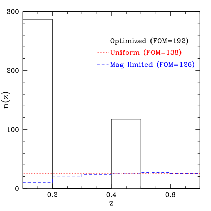
The FOM becomes a quite respectable 192, with determination of $\Omega_{m}$ to 0.0035, $w_{0}$ to 0.061, $w_{a}$ to 0.22, and $h$ to $0.0030$. Each parameter estimation, as well as the FOM, is better than for either the uniform redshift distribution or a magnitude limited distribution derived from ogurimars using cuts on image and lens flux and image separation (P. Marshall, S. Suyu private communication). We have tested reducing the redshift range to 0.1–0.4 or 0.1–0.5, and obtain the same optimized distribution, i.e. the optimum really has only the low and mid redshift bin. We also shifted the range to $z=0.2$–0.7 and found the optimized FOM dropped significantly, to 135, demonstrating the lowest bin is critical for dark energy as well as the Hubble constant.

IV Influence of Systematics

Any cosmological probe must deal with systematic uncertainties, especially for next generation surveys where abundant numbers of objects drive down the statistical uncertainty. We investigate two of the manifold aspects of the impact of systematics. Again, a detailed treatment would need to delve deep into survey and instrumentation properties, and is beyond the present scope.

IV.1 Redshift distribution revisited

Let us explore the effect of systematic uncertainties on the optimization carried out in Sec. III. The number of lens systems in the lowest redshift bin approached 300, which for individual system precision of 5% implies a required control of systematic bias at the 0.3% level. We do not yet know enough from current strong lensing observations and studies to know what is a realistic level, but strong efforts and advances in understanding are underway. For example, the blind data Time Delay Challenge (http://timedelaychallenge.org) has already achieved 0.1–0.2% control of time delay estimation tdc0 ; tdc1 ; hoj ; amir .

Therefore we study the impact of various levels of systematic on the optimized redshift distribution and the resulting cosmological parameter estimation. We implement the systematic as a floor, added in quadrature to the statistical uncertainty,

$$\frac{\sigma^{2}}{n_{i}}=\frac{\sigma^{2}_{\rm stat}}{n_{i}}+\sigma^{2}_{\rm sys}\ ,$$ (6)

where $n_{i}$ is the number in redshift bin $i$ and each bin is treated independently. This model is commonly used in supernova distance-redshift relation studies klmm . (But see the next subsection for an alternative approach to systematics.)

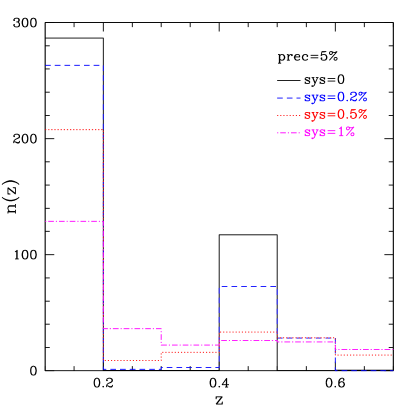
Figure 2 shows the optimized distributions, subject to the resource constraint, for different levels of systematic. As the systematic level increases, it is less advantageous to put a large number of systems in a given redshift bin and additional systems diffuse into neighboring bins. This fills in the intermediate redshift gap and also pushes some lens systems to high redshift, making the distribution closer to uniform.

Figure 2: The resource-constrained optimization of the lens redshift distribution is shown as a function of coherent distance systematic floor. This floor prevents large numbers of systems in a redshift bin from improving the accuracy.

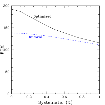
Both the presence of the systematic and the redistribution of the data away from the zero-systematic optimum lowers the FOM. Figure 3 plots the FOM vs the systematic level. At 0.2% systematic, the FOM has decreased by only 8% relative to zero systematic case, but larger systematics impact the cosmology more severely. For high enough levels, there is little difference in leverage between the optimized and uniform (or magnitude limited) distributions.

Figure 3: Dark energy figure of merit is plotted for the optimized cosmological leverage and uniform lens redshift distributions as a function of systematic floor. For high systematics, the optimized distribution has little extra leverage, but at low systematics the improvement can approach 40%.

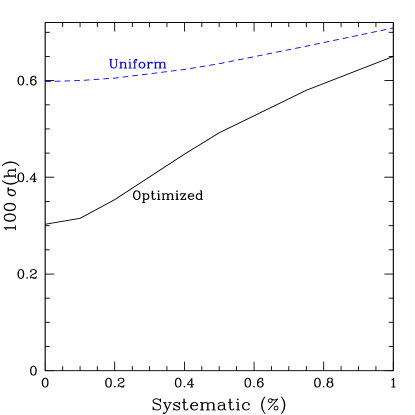
To make sure that optimizing for dark energy FOM also helps improve other cosmological parameters, we show in Fig. 4 the constraint on the Hubble constant $h$. For zero systematic the optimization actually improves the estimation by a factor 2 (not just 40% as for the FOM). This is because the increased low redshift sample is particularly useful for the Hubble constant. Even for higher levels of systematics the optimization continues to give added leverage on $h$.

Figure 4: As Fig. 3 but for the Hubble constant constraint (note that here low values are better). At high systematics, the optimization still improves the results by almost 10%, while at low systematics the gain is a factor 2.

IV.2 Model systematics

Statistical uncertainties in the time delay distance arise from measurement imprecision, but the measurement errors can have systematic components as well. These take two main forms: correlated errors between elements in a given lensed system, and model errors that are common between different lens systems. These will give diagonal and offdiagonal contributions to the distance error matrix. Below we give an illustrative exhibition of the effect of such systematics; again, actual survey analysis requires a more detailed and sophisticated treatment but this demonstrates the main points.

Let us write the time delay distance as

$$D_{\Delta t}=D_{\Delta t}(\Delta t,\Delta\phi(m,\vec{\theta},\Delta t,v,z),\kappa_{\rm ext})\ ,$$ (7)

where the Fermat potential depends on image magnitudes $m$, positions $\vec{\theta}$, time delays $\Delta t$, lens and image redshifts $z$, and lens velocity dispersion $v$. Additional mass along the line of sight affects the modeling through the external convergence $\kappa_{\rm ext}$.

Ref. suyu13 demonstrates that over the angular range important for the images, i.e. near the Einstein radius of the lens, the Fermat potential scales with the projected lens mass profile slope $\gamma^{\prime}$. Even when the galaxy lens profile has a multicomponent composition sluse of a Hernquist stellar core plus a Navarro-Frenk-White dark matter profile, over the angular range of interest the slope $\gamma^{\prime}$ captures the profile dependence. Uncertainties or misestimation in $\gamma^{\prime}$ then lead to dispersion or systematics in the Fermat potential and hence the distances. There is also a mass sheet degeneracy due to mass along the line of sight. Both these effects can be incorporated through suyu13

$$\phi\approx\bar{\phi}\,(1-\kappa_{\rm ext})(\gamma^{\prime}-1)\ ,$$ (8)

in the vicinity of the standard profile slope $\gamma^{\prime}=2$. Note that systems measured to date have rms dispersion of $\lesssim 5\%$ in $\gamma^{\prime}$ so this form is accurate.

We can now write the time delay distance as

$$D_{\Delta t}=\frac{\Delta t}{\bar{\phi}(m,\vec{\theta},\Delta t,v,z)\,(1-\kappa_{\rm ext})(\gamma^{\prime}-1)}\ .$$ (9)

The error propagation to the time delay distance, for accurate image flux and position measurements, is then

$$\delta D=D_{t}\delta t+D_{v}\delta v+D_{z}\delta z+D_{\kappa}\delta\kappa+D_{\gamma}\delta\gamma\ ,$$ (10)

where we use the simplifying notation $D=D_{\Delta t}$, $D_{x}$=$\partial D/\partial x$, and $\gamma=\gamma^{\prime}$, $\kappa=\kappa_{\rm ext}$, $t=\Delta t$.

A reasonable first approach, based on current data, is that the error budget will be dominated by the time delay estimation, external convergence, and lens mass profile and velocity dispersion. In this case the diagonal entries in the error matrix (i.e. for a single lens system) would be

$$C_{DD} \approx D^{2}_{t}\sigma^{2}_{t}+D^{2}_{v}\sigma^{2}_{v}+D^{2}_{\kappa}\sigma^{2}_{\kappa}+D^{2}_{\gamma}\sigma^{2}_{\gamma}$$ (11)

$$+D_{v}D_{\gamma}\langle\delta v\,\delta\gamma\rangle+D_{\kappa}D_{\gamma}\langle\delta\kappa\,\delta\gamma\rangle\ .$$

This reflects the individual errors, plus the correlated errors between $v$ and $\gamma$ in the lens density profile (e.g. whether $v$ is measured at the appropriate place in the profile), and between $\gamma$ and $\kappa$ in the profile-mass sheet degeneracy. We emphasize this is illustrative.

The model errors enter in the off diagonal elements. Recall these correlate two different lens systems at distances $D$ and $D^{\prime}$. Here the error matrix gets the contribution

$$C_{DD^{\prime}} = D_{t}D^{\prime}_{t}\langle\delta t\,\delta t^{\prime}\rangle+D_{v}D^{\prime}_{v}\langle\delta v\,\delta v^{\prime}\rangle+D_{\kappa}D^{\prime}_{\kappa}\langle\delta\kappa\,\delta\kappa^{\prime}\rangle$$ (12)

$$+ D_{\gamma}D^{\prime}_{\gamma}\langle\delta\gamma\,\delta\gamma^{\prime}\rangle+D_{v}D^{\prime}_{\gamma}\langle\delta v\,\delta\gamma^{\prime}\rangle+D^{\prime}_{v}D_{\gamma}\langle\delta v^{\prime}\,\delta\gamma\rangle$$

$$+ D_{\kappa}D^{\prime}_{\gamma}\langle\delta\kappa\,\delta\gamma^{\prime}\rangle+D^{\prime}_{\kappa}D_{\gamma}\langle\delta\kappa^{\prime}\,\delta\gamma\rangle\ .$$

Several of the derivatives can be written in a straightforward manner using Eq. (9):

$$D_{t} = \frac{D}{\Delta t}\quad;\quad D_{\gamma}=-\frac{D}{\gamma-1}$$ (13)

$$D_{\kappa} = \frac{D}{1-\kappa_{\rm ext}}\quad;\quad D_{v}=D_{\phi}\frac{\partial\phi}{\partial v}\approx-2\frac{D}{v}\ .$$

The approximation sign in $D_{v}$ represents the result for a singular isothermal sphere.

Once we are in the regime of thousands of strong lenses coemous ; ogurimars , the $\sqrt{N}$ statistical reduction will be dominated by the residual systematics. It is crucial to identify the effects of these systematics on cosmological results, and where the greatest leverage lies in controlling them. This has significant interplay with our previous analysis of constrained followup resources. That is, we want to identify where best to concentrate the limited resources, e.g. on long time delay, quad image systems. One example is that double images often occur at different radii where the lens slope profile may vary, while quads suffer less from such a systematic. Quad systems may have better precision from the extra measurement constraints, but possibly also an increased opportunity for differential microlensing or varying external convergence.

For a tractable first approach, we note that Eqs. (11), (12), and (13) have the property that the uncertainties often enter into the error covariance matrix as logarithmic fractional quantities, i.e. $\delta\gamma^{\prime}/(\gamma^{\prime}-1)$ or $\delta\kappa/(1-\kappa)$, times the time delay distance. We adopt the Ansatz that these fractional systematic uncertainties have a scaling with redshift $s=s_{\star}\,[(1+z)/(1+z_{\star})]^{n}$, where $z_{\star}=0.4$ is the midpoint of the redshift range, and a possible population dependence, where the errors in double systems may differ from those in quad systems. Since the fraction of doubles vs quads detected in a survey changes with redshift, this causes a population drift in a manner similar to supernova subtype evolution.

The overall covariance matrix will then have two entries in each redshift bin, for doubles and quads, with distinct statistical and systematic errors. We sum up all the statistical errors from the time delay estimation, mass profile slope, etc. to give diagonal entries of $\sigma^{2}_{\{d,q\}}(z_{i})\,D_{i}^{2}$ in the $i$th lens redshift bin. Here $D_{i}$ is the time delay distance of Eq. (1). The systematic errors $s_{\{d,q\}}(z_{i})\,D_{i}$ also contribute to the diagonal elements and moreover their correlations produce offdiagonal entries. While in actual data analysis one might not bin the data, and the error model will become more sophisticated over time, this approach using five parameters ($\sigma_{d}$, $\sigma_{q}$, $s_{d}$, $s_{q}$, and $n$ if desired) is tractable and gives important first indications of the effect of systematics.

We first discuss direct redshift evolution of the systematics, and then the influence of population drift.

Figure 5 shows the influence of the redshift dependence of the systematic. In order to focus on the redshift evolution of the systematic, we here take the uniform redshift distribution of Sec. III (despite its lower FOM), and treat all populations (doubles or quads) as having 5% statistical precision in distance and a fractional distance systematic $s$ per redshift bin. The evolution in $s$ with redshift could arise from, e.g., decreased signal to noise, and hence more uncertain modeling, of higher redshift lens systems (and a longer path length so greater uncertainty in the projected mass along the line of sight).

Figure 5: The dark energy figure of merit (solid curves) and Hubble constant uncertainty (dashed curves) are shown as a function of systematic error amplitude $s_{\star}$ at $z_{\star}=0.4$, for three different redshift evolutions. The systematic scales as $(1+z)^{n}$ for $n=0$, 1, 2. Note that high figure of merit is good, and low $\sigma(h)$ is good.

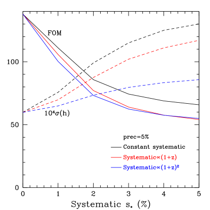
We see that the specific systematic redshift evolution model, as opposed to the mere presence of the systematic, has a modest effect, with the variation among $n=0-2$ affecting the dark energy figure of merit by $\sim 20\%$ and determination of the Hubble constant by $\sim 50\%$ at the highest systematic levels. Note that the evolution does change the covariance between parameters; this is responsible for the $n=1$ and $n=2$ curves crossing at high systematic. Although $w_{0}$ and $w_{a}$ are both better determined in the $n=1$ case, the FOM is not, due to their altered covariance. As expected, a constant fractional systematic has more of an effect on $h$, and so less on the FOM.

As a next step, we include separate systematics for the populations of double and quad image systems. Again the motivation is that these have different levels of constraints on the lens model from the observations, e.g. image positions, flux ratios, number of time delays. To focus on this population aspect, we keep the explicit systematic amplitude independent of redshift ($n=0$; recall we just saw that the cosmology constraints were fairly insensitive to $n$ anyway) but incorporate population drift with redshift.

The distribution of doubles and quads we use is the magnitude limited sample of Sec. III, based on ogurimars (again for illustration, despite its lower FOM). This arises from the constraints that 1) image separation is larger than $1^{\prime\prime}$, 2) the quasar images are brighter than i-magnitude 20.8, and 3) the lens magnitude is brighter than 22. These help ensure that images and arcs can be well resolved, time delays can be accurately measured, and the lens velocity dispersion can be measured with reasonable use of resources. The ratio of doubles to quads varies from roughly 9 to 4 from the low to high end of the redshift range, with statistical scatter in numbers included. The drift in the proportion leads to an effective redshift evolution in the systematic uncertainty, analogously to how population drift of supernovae subtypes with slightly different absolute magnitudes engenders supernova magnitude evolution (see likesys ; johansys for detailed treatment of the propagation of this effect into cosmology constraints).

Figure 6 quantifies how population drift between the double image and quad image systems propagates into cosmological constraints as the amplitude and ratio of the double and quad systematic errors varies. The top panel fixes $s_{q}=1\%$ and varies $s_{d}$, while the bottom panel fixes $s_{d}=4\%$ and varies $s_{q}$. As the systematic level increases, the dark energy figure of merit decreases and the uncertainty in the determination of the Hubble constant increases, as expected. However, when the systematic error of the doubles exceeds their statistical uncertainty, then the information from the doubles saturates, the quads dominate the leverage, and the FOM and $\sigma(h)$ level off (see top panel). This implies that systematics in doubles have a natural “knee” – defining when the limited observational resources have greater leverage when used to accurately characterize the rarer quad systems. The bottom panel shows that as long as the quad systematic is lower than its statistical uncertainty, then more accurate measurement of quads leads to more stringent cosmological constraints. Such an analysis can inform the optimal use of resources for strong lensing time delay distances as a cosmological probe.

Figure 6: [Top panel] The dark energy figure of merit (solid curve) and Hubble constant uncertainty (dashed curve) are shown as a function of fractional systematic error $s_{d}$ in double image systems, for a fixed quad image systematic $s_{q}=0.01$. [Bottom panel] As the top panel, but as a function of $s_{q}$ for fixed $s_{d}=0.04$.

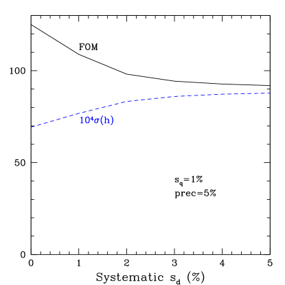
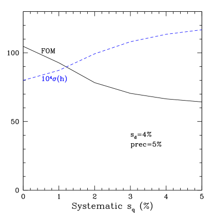
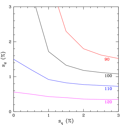
Figure 7 depicts the results for simultaneous variation of the double and quad systematics, showing contours of constant FOM. At high systematics level, having the two contributions be comparable gives the best FOM. However at low systematics level we are below the quad statistical uncertainty. This gives two approaches for improvement: either improving the doubles systematic or allocating more resources to followup more quad systems and bring down their statistical error. From the distance between the contours, we see that if low quad systematics can be achieved, then considerable improvement in doubles systematics is required for significant improvement; thus following up more quad systems seems a better option in this case.

Figure 7: Contours of constant FOM are plotted as a function of the systematic levels in double and quad lensing systems. The zero systematics point has FOM=126.

V Conclusions

The strong gravitational lensing time delay distance-redshift relation is a geometric probe of cosmology. It has two particularly valuable characteristics: being dimensionful and hence sensitive to the Hubble constant $H_{0}$, and being a triple distance ratio and hence with different parameter degeneracies that make it highly complementary to other distance probes such as the cosmic microwave background or supernovae. Moreover, the observations and modeling are rapidly advancing, enabling it to place cosmological constraints of significant leverage, comparable to other methods.

We considered the question of the followup resources needed to complement the forthcoming strong lensing imaging surveys that detect and monitor the lens systems. Since high resolution imaging or spectroscopic followup is limited and expensive, we optimized the lens system redshift distribution to give maximal cosmology leverage. The optimization code under fixed resources such as spectroscopic time (e.g. to measure the lens galaxy velocity dispersion to constrain the lens mass model) is computationally fast and efficient, with its algorithm generally applicable to many astrophysical studies and figures of merit.

The sculpted distribution delivers a nearly 40% improvement in dark energy figure of merit, and a factor two tighter constraint on the Hubble constant, than a uniform redshift distribution. Low redshift systems are found to be particularly preferred, and there is no need to spend followup time on lenses with $z>0.5$.

Systematics enter as correlated quantities within a given lensing system, and as model systematics common to many systems. We examined both in an illustrative model that captures key aspects. A systematic uncertainty floor somewhat spreads out the optimal redshift distribution, but preserves the advantage of low redshift. We then demonstrated the effects of both a systematic explicitly evolving in redshift and one caused by population drift between different lens system types, such as double image vs quad image systems. If the systematic level for one population is larger than for the other, we can quantify by how much the followup resources are better spent on the more accurate population.

As wide field surveys deliver 1000–10000 strong lensing systems, the issue of followup will become a key limitation, and these optimization tools can significantly improve the cosmological leverage. Similarly, as our measurement of strong lensing systems improves, the illustrative systematic correlation model here will become more realistic and enable more sophisticated trade studies regarding low vs high redshift, or double vs quad image systems. This will further optimize future surveys to use strong lensing time delay distances as a unique cosmological probe.