Computation of Local Time of Reflecting Brownian Motion and Probabilistic Representation of the Neumann Problem

Abstract

In this paper, we propose numerical methods for computing the boundary local time of reflecting Brownian motion (RBM) in $\displaystyle R^{3}$ and its use in the probabilistic representation of the solution of the Laplace equation with the Neumann boundary condition. Approximations of the RBM based on a walk-on-spheres (WOS) and random walk on lattices are discussed and tested for sampling the RBM paths and their applicability in finding accurate approximation of the local time and discretization of the probabilistic formula. Numerical tests for several types of domains (cube, sphere, and ellipsoid) have shown the convergence of the numerical methods as the length of the RBM path and number of paths sampled increase.

, ,

Suggested Running Head:
Local Time of Reflecting Brownian Motion and Probabilistic Representation of the Neumann Problem

Corresponding Author:
Prof. Wei Cai
Department of Mathematics and Statistics,
University of North Carolina at Charlotte,
Charlotte, NC 28223-0001
Phone: 704-687-0628, Fax: 704-687-6415,
Email: wcai@uncc.edu

AMS Subject classifications: 65C05, 65N99, 78M25, 92C45

1 Introduction

Traditionally numerical solutions of boundary value problems for partial differential equations (PDEs) are obtained by using finite difference, finite element or boundary element methods with both space and/or time discretizations. This usually requires spatial mesh fine enough to ensure accuracy, which results in considerable storage space requirement and computation time. Moreover, the solution process is global, namely, the solutions of the PDEs have to be found together at all mesh points. However, in many scientific and engineering applications, local solutions are sometimes all we need, such as the local electrostatic potential on a molecular surface where molecular binding activities are most likely to occur or the stress field at specific locations where the materials are susceptive to failures. Therefore, it is of practical importance to have a numerical approach which can give a local solution of the PDEs at some locality of our choice. In the case of elliptic PDEs, this kind of local numerical method can be constructed using the well-known probabilistic representation and the associated Feynman-Kac formula [16][17], which relate Itô diffusion paths to the solution of the elliptic PDEs. By sampling the diffusion paths, the evaluation of the solution at any point in the domain can be done through an averaging process of the boundary (Dirichlet or Neumann) data under some given measure on the boundary. Moreover, this method avoids the expensive mesh generations required by mesh-based methods mentioned above [15].

Our previous work [4] , using the Feynman-Kac formula for the Laplace equation with Dirichlet data, has produced a local method to compute the DtN (Dirichlet-to-Neumann) mapping for the Laplace operator. In this paper, we will focus on solving the following Neumann boundary value problem of the elliptic PDE using a probabilistic approach:

$$\left\{\begin{aligned} \Delta u&=f,\ on\ D\\ \frac{\partial u}{\partial n}&=\phi,\ on\ \partial D\\ \end{aligned}\right.,$$ (1)

where $\displaystyle D$ is a bounded domain in $\displaystyle R^{3}$, $\displaystyle\Delta$ is the Laplace operator, $\displaystyle f$ is a measurable function and $\displaystyle\phi$ is a bounded measurable function on the boundary $\displaystyle\partial D$ satisfying $\displaystyle\int_{\partial D}\phi d\sigma=\int_{D}fdx$. Equation $\displaystyle(1)$ becomes the Laplace equation when $\displaystyle f=0$, which is the subject of our work.

The PDE (1) originates from either the Poisson equation for electrostatic potentials [19], an implicit time discretization of the heat equation or the momentum equation of the Naiver-Stokes equation with an additional lower term in the latter cases. Historically, Brownian motion (BM) has been used in solving PDEs due to its effectiveness and easy implementation regardless of dimensions [10]. The well-known probabilistic representation can solve the elliptic equation with the Dirichlet boundary condition by using the first exit time $\displaystyle\tau_{D}$ of BM, i.e.,

$$u(x)=E^{x}(\phi(x_{\tau_{D}}))+E^{x}\left[\int_{0}^{\tau_{D}}f(X_{t})dt\right].$$ (2)

In the above formula, only the values at the hitting positions on the boundary are used in the computation of the mathematical expectation (average) to obtain $\displaystyle u(x)$. Taking the idea of killed Brownian motion [4] in junction with Monte Carlo methods, we can easily obtain an estimate of $\displaystyle u(x)$.

However, for the Neumann problem to be studied here, in contrast to the Brownian motion in (2), reflecting Brownian motion (RBM) will be needed to produce a similar probabilistic solution to (1). This theory has been developed in [1] by employing the concept of the boundary local time whose one dimensional predecessor was introduced by Lévy in [3]. In [1], the boundary local time of a one dimensional BM was extended to high dimensions and an explicit form, shown in (6), was obtained for domains with smooth boundaries. It should be noted that the boundary local time is related to the Skorohod equation [14] and plays a significant role in the theoretical development of the probabilistic approach to the Neumann problem.

One-dimensional local time of Brownian motion has been studied by many authors [3][11][13][14]. For higher dimensions, similar results have been found by Brosamler [2]. Morillon [8] gave a modified Feynman-Kac formula for the Poisson problem with various boundary conditions, algorithms based on random walk on a grid have been proposed. However, numerical algorithms for computing local time in $\displaystyle R^{3}$ based on a rigorous probabilistic theory has not been done in the literature. It is the objective of this paper to obtain practical numerical methods for computing the local time of RBM in three dimensions and apply the resulting numerical methods to implement computationally the probabilistic representation for the Neumann problem.

The rest of the paper is organized as follows. In section 2, we give some background information on the Skorohod problem which is the key to the Neumann problem. In section 3, an explicit probabilistic solution to the Neumann problem will be given. In section 4, a walk-on-spheres (WOS) method is reviewed and discussed for its application for RBM. In section 5, a numerical method, the WOS combined with a Monte Carlo method, is proposed for an approximation to the Neumann problem. Numerical results for cubic, spherical and ellipsoidal domains will be given in Section 6. Finally, we draw conclusions from our Monte Carlo simulations and discuss possible further work.

2 Skorohod Problem, RBM and Boundary Local Time

For the sake of completeness, we first give the definitions of Brownian motion and reflecting Brownian motion in $\displaystyle R^{d}$.

Definition 1

Brownian motion: A Brownian motion $\displaystyle B(t)=(B_{1}(t),B_{2}(t),...,B_{d}(t))$ in $\displaystyle R^{d}$ is a set of $\displaystyle d$ independent stochastic processes with the following properties: for $\displaystyle 1\leq i\leq d$,

1. (Normal increments) $\displaystyle B_{i}(t)-B_{i}(s)$ has a normal distribution with mean 0 and variance $\displaystyle t-s$.

2. (Independence of increments) $\displaystyle B_{i}(t)-B_{i}(s)$ is independent of the past, i.e., of $\displaystyle B_{u}$, $\displaystyle 0\leq u\leq s$.

3. (Continuity of paths) $\displaystyle B_{i}(t),t\geq 0$ is a continuous function of $\displaystyle t$.

Definition 2

Skorohod equation: Assume $\displaystyle D$ is a bounded domain in $\displaystyle R^{d}$ with a $\displaystyle C^{2}$ boundary. Let $\displaystyle f(t)$ be a (continuous) path in $\displaystyle R^{d}$ with $\displaystyle f(0)\in\bar{D}$. A pair $\displaystyle(\xi_{t},L_{t})$ is a solution to the Skorohod equation $\displaystyle S(f;D)$ if the following conditions are satisfied:

1. $\displaystyle\xi$ is a path in $\displaystyle\bar{D}$;

2. $\displaystyle L(t)$ is a nondecreasing function which increases only when $\displaystyle\xi\in\partial D$, namely,

   $$L(t)=\int_{0}^{t}I_{\partial D}(\xi(s))L(ds);$$ (3)

3. The Skorohod equation holds:

   $$S(f;D):\qquad\ \xi(t)=f(t)-\frac{1}{2}\int_{0}^{t}n(\xi(s))L(ds),$$ (4)

   where $\displaystyle n(x)$ stands for the outward unit normal vector at $\displaystyle x\in\partial D$.

Remark 3

In Definition 2, the smoothness constraint on $\displaystyle D$ can be relaxed to bounded domains with $\displaystyle C^{1}$ boundaries, which however will only guarantee the existence of $\displaystyle(\ref{eq7})$. But for a domain $\displaystyle D$ with a $\displaystyle C^{2}$ boundary, the solution will be unique. Obviously, $\displaystyle(\xi_{t},L_{t})$ is continuous in the sense that each component is continuous.

If $\displaystyle f(t)$ is replaced by the standard Brownian motion (BM) $\displaystyle B_{t}$, the corresponding $\displaystyle\xi_{t}$ will be a standard reflecting Brownian motion (RBM) $\displaystyle X_{t}$. Just as the name suggests, a reflecting BM (RBM) behaves like a BM as long as its path remains inside the domain $\displaystyle D$, but it will be reflected back inwardly along the normal direction of the boundary when the path attempts to pass through the boundary. The fact that $\displaystyle X_{t}$ is a diffusion process with the Neumann boundary condition can be proven by using a martingale formulation and showing that $\displaystyle X_{t}$ is the solution to the corresponding martingale problem with the Neumann boundary condition [1]. The result gives an intuitive and direct way to construct RBM from BM. This construction will be discussed in detail in Section 5.

Next we will review the concept of boundary local time $\displaystyle L(t)$ for a RBM, which in a sense is a measure of the amount of time a RBM spends near the boundary and at the same time the frequency that a RBM hits the boundary. We have the following properties of $\displaystyle L(t)$:

1. It is the unique continuous nondecreasing process that appears in the Skorohod equation (4) [1];

2. It measures the amount of time the standard reflecting Brownian motion $\displaystyle X_{t}$ spending in a vanishing neighborhood of the boundary within the period $\displaystyle[0,t]$. If $\displaystyle D$ has a $\displaystyle C^{3}$ boundary, then

   $$L(t)\equiv\lim_{\epsilon\rightarrow 0}\frac{\int_{0}^{t}I_{D_{\epsilon}}(X_{s})ds}{\epsilon},$$ (5)

   where $\displaystyle D_{\epsilon}$ is a strip region of width $\displaystyle\epsilon$ containing $\displaystyle\partial D$ and $\displaystyle D_{\epsilon}\subset D$. This limit exists both in $\displaystyle L^{2}$ and $\displaystyle P^{x}$-$\displaystyle a.s$. for any $\displaystyle x\in\overline{D}$;

3. $\displaystyle L(t)$ is a continuous additive functional (CAF) [2] which satisfies the additivity property [1][2][13][14]: $\displaystyle A_{t+s}=A_{s}+A_{t}(\theta_{s})$. Here $\displaystyle\theta_{s}$ denotes the shift operator along the paths. The additivity property of $\displaystyle L(t)$ can be seen as follows:

   From the definition in (5), we have

   $$\left\{\begin{aligned} L(t+s)&=\lim_{\epsilon\rightarrow 0}\frac{\int_{0}^{t+s}I_{D_{\epsilon}}(X_{\tau})d\tau}{\epsilon}\\ L(s)&=\lim_{\epsilon\rightarrow 0}\frac{\int_{0}^{s}I_{D_{\epsilon}}(X_{\tau})d\tau}{\epsilon}\\ L(t)\circ\theta_{s}&=\lim_{\epsilon\rightarrow 0}\frac{\int_{0}^{t}I_{D_{\epsilon}}(X_{\tau+s})d\tau}{\epsilon}=\lim_{\epsilon\rightarrow 0}\frac{\int_{s}^{t+s}I_{D_{\epsilon}}(X_{\tau})d\tau}{\epsilon}\end{aligned}\right.,$$

   therefore,

   $$L(t+s)=L(t)+L(t)\circ\theta_{s},$$

   which shows that $\displaystyle L(t)$ satisfies the additivity property.

For one-dimensional case, much existing literature devoted to the study of local times for Brownian motion and more general diffusion processes. It is well known that for one dimensional Brownian motion starting from the origin, the local time $\displaystyle L(t)$ of RBM and $\displaystyle\max_{s\leq t}B(s)$ have the same distribution as stochastic processes. Hence, valuable properties of RBM can be drawn by just observing $\displaystyle\max_{s\leq t}B(s)$. But this is not true in general in higher dimensions. However, we have the following explicit formula for $\displaystyle L(t)$ derived in [1],

$$L(t)=\sqrt{\frac{\pi}{2}}\int_{0}^{t}I_{\partial D}(X_{s})\sqrt{ds},$$ (6)

where the the right-hand side of (6) is understood as the limit of

$$\sum_{i=1}^{n-1}\smash{\displaystyle\max_{s\in\Delta_{i}}I_{\partial D}(X_{s})\sqrt{|\Delta_{i}|}},\quad\smash{\displaystyle\max_{i}}|\Delta_{i}|\rightarrow 0,$$ (7)

where $\displaystyle\Delta=\{\Delta_{i}\}$ is a partition of the interval $\displaystyle[0,t]$ and each $\displaystyle\Delta_{i}$ is an element in $\displaystyle\Delta$. We will discuss the implementation of both (5) and (6) in Section 5.

3 Neumann Problem

We will consider the elliptic PDE in $\displaystyle R^{3}$ with a Neumann boundary condition

$$\left\{\begin{aligned} \left(\frac{\Delta}{2}+q\right)u&=0,\ on\ D\\ \frac{\partial u}{\partial n}&=\phi,\ on\ \partial D\\ \end{aligned}\right..$$ (8)

When the bottom of the spectrum of the operator $\displaystyle\Delta/2+q$ is negative a probablistic solution of $\displaystyle(\ref{eq17})$ is given by

$$u(x)=\frac{1}{2}E^{x}\left[\int_{0}^{\infty}e_{q}(t)\phi(X_{t})L(dt)\right],$$ (9)

where $\displaystyle X_{t}$ is a RBM starting at $\displaystyle x$ and $\displaystyle e_{q}(t)$ is the Feynman-Kac functional [1]

$$e_{q}(t)=\exp\left[\int_{0}^{t}q(X_{s})\,ds\right].$$

From the definition of the local time in (5), we have the following approximation for small $\displaystyle\epsilon$

$$L(t)\approx\frac{\int_{0}^{t}I_{D_{\epsilon}}(X_{s})ds}{\epsilon}.$$ (10)

Plugging $\displaystyle(\ref{eq21})$ into $\displaystyle(\ref{eq19})$, we have

$$u(x)\approx\frac{1}{2\epsilon}E^{x}\left[\int_{0}^{\infty}e_{q}(t)\phi(X_{t})\int_{t}^{t+dt}I_{D_{\epsilon}}(X_{s})ds\right].$$ (11)

The solution defined in $\displaystyle(\ref{eq19})$ should be understood as a weak solution for the classical PDE $\displaystyle(\ref{eq17})$. The proof of the equivalence of (9) with a classical solution is done by using a martingale formulation [1]. If the weak solution satisfies some smoothness condition [1][2], it can be shown that it is also a classical solution to the Neumann problem. This formula is the basis for our numerical approximations to the Neumann problem $\displaystyle(\ref{eq17})$. To compute the expectation in the formula, we rely on Monte Carlo random samplings to simulate Brownian paths and then take the average.

In the present work, as we only consider the Laplace equation where $\displaystyle q=0$, therefore,

$$u(x)\approx\frac{1}{2\epsilon}E^{x}\left[\int_{0}^{\infty}\phi(X_{t})\int_{s}^{s+dt}I_{D_{\epsilon}}(X_{s})ds\right],$$ (12)

and we will show how this formula is implemented with the Monte Carlo and WOS methods in section 5.

Remark 4

Comparing with formula $\displaystyle(\ref{eq19})$, we find that the probabilistic solutions to the Laplace operator with the Dirichlet boundary condition has a very similar form (referring to $\displaystyle(\ref{eq29})$). In the Dirichlet case, killed Brownian paths were sampled by running random walks until the latter are absorbed on the boundary and $\displaystyle u(x)$ is evaluated as an average of the Dirichlet values at the first hitting positions on the boundary, namely, $\displaystyle u(x)=E^{x}\left[\phi(X_{\tau_{D}})\right]$ where $\displaystyle\phi$ is the Dirichlet boundary data. On the other hand, for the Neumann condition, while $\displaystyle u(x)$ is also given as a weighted average of the Neumann data at hitting positions of RBM on the boundary, the weight is related to the boundary local time of RBM. This is a noteworthy point when we compare the probabilistic solutions of the two boundary value problems and try to understand the formula in $\displaystyle(\ref{eq19})$.

4 Method of Walk on Spheres (WOS)

Random walk on spheres (WOS) method was first proposed by Müller [7], which can solve the Dirichlet problem for the Laplace operator efficiently. Here we will first briefly review this method and then show how it can be adapted for RBM and the Neumann problem.

For a general linear elliptic problem with a Dirichlet boundary condition,

$$L(u)=\sum_{i=1}^{n}b_{i}(x)\frac{\partial u}{\partial x_{i}}+\sum_{i,j=1}^{n}a_{ij}(x)\frac{\partial^{2}u}{\partial x_{i}\partial x_{j}}=f(x),x\in D,$$ (13)

$$u|_{\partial D}=\phi(x),x\in\partial D.$$

The probabilistic representation of the solution is ([16][17])

$$u(x)=E^{x}(\phi(x_{\tau_{D}}))+E^{x}\left[\int_{0}^{\tau_{D}}f(X_{t})dt\right],$$ (14)

where $\displaystyle X_{t}(w)$ is an Itô diffusion defined by

$$dX_{t}=b(X_{t})dt+\alpha(X_{t})dB_{t},$$ (15)

and $\displaystyle B_{t}(w)$ is the Brownian motion, $\displaystyle[a_{ij}]=\frac{1}{2}\alpha(x)\alpha^{T}(x)$.

The expectation in (14) is taken over all sample paths starting from $\displaystyle x$ and $\displaystyle\tau_{D}$ is the first exit time for the domain $\displaystyle D$. This representation holds true for general linear elliptic PDEs. For the Neumann boundary condition, similar formulas can be obtained [8]. However different measures on the boundary $\displaystyle\partial D$ will be used in the mathematical expectation.

In order to illustrate the WOS method for the Dirichlet problem, let us consider the Laplace equation where $\displaystyle f=0,a_{ij}=\delta_{ij}$ and $\displaystyle b_{i}=0$ in (13) and the Itô diffusion is then simply the standard Brownian motion with no drift. The solution to the Laplace equation can be rewritten in terms of a measure $\displaystyle\mu_{D}^{x}$ defined on the boundary $\displaystyle\partial D$,

$$u(x)=E^{x}(\phi(X_{\tau_{D}}))=\int_{\partial D}\phi(y)d\mu_{D}^{x},$$ (16)

where $\displaystyle\mu_{D}^{x}$ is the so-called harmonic measure defined by

$$\mu_{D}^{x}(F)=P^{x}\left\{X_{\tau_{D}}\in F\right\},F\subset\partial D,x\in D.$$ (17)

It can be shown that the harmonic measure is related to the Green’s function for the domain with a homogeneous boundary condition,

$$\left\{\begin{aligned} -\Delta g(x,y)&=\delta(x-y),\ &x\in D,\\ g(x,y)&=0,\ &x\in\partial D\\ \end{aligned}\right..$$ (18)

By the third Green’s identity,

$$u(x)=\int_{\partial D}\left[u(y)\frac{\partial g(y,x)}{\partial n}-g(y,x)\frac{\partial u}{\partial n}(y)\right]dS_{y},$$ (19)

and using the zero boundary condition of $\displaystyle g$, we have

$$u(x)=\int_{\partial D}u(y)\frac{\partial g(y,x)}{\partial n}dS_{y}.$$ (20)

Thus, the hitting probability $\displaystyle\mu_{D}^{x}([y,y+dS_{y}])$ is equivalent to $\displaystyle p(x,y)dS_{y}$. Comparing (16) with (20), we can see that

$$p(\mathbf{x},\mathbf{y})=-\frac{\partial g(x,y)}{\partial n_{y}}.$$ (21)

For instance, the Green’s function for a ball for this purpose is given as

$$g(x,y)=-\frac{1}{4\pi|x-y|}+-\frac{1}{4\pi|x-y^{\ast}|},$$ (22)

where $\displaystyle y^{\ast}$ is the inversion point of $\displaystyle y$ with respect to the sphere [4].

If the starting point $\displaystyle x$ of a Brownian motion is at the center of a ball, the probability of the BM exiting a portion of the boundary of the ball will be proportional to the portion’s area. It is known that all sample functions of Brownian motion processes starting in the domain intersects the boundary $\displaystyle\partial D$ almost surely [7]. Therefore, sampling a Brownian path by drawing balls within the domain, regardless of how the path navigates in the interior before hitting the boundary, can significantly reduce the path sampling time. To be more specific, given a starting point $\displaystyle x$ inside the domain $\displaystyle D$, we simply draw a ball of largest possible radius fully contained in $\displaystyle D$ and then the next location of the Brownian path on the surface of the ball can be sampled, using a uniform distribution on the sphere, say at $\displaystyle x_{1}$. Treat $\displaystyle x_{1}$ as the new starting point, draw a second ball fully contained in $\displaystyle D$, make a jump from $\displaystyle x_{1}$ to $\displaystyle x_{2}$ on the surface of the second ball as before. Repeat this procedure until the path hits a absorption $\displaystyle\epsilon$-shell of the domain [5]. When this happens, we assume that the path has hit the boundary $\displaystyle\partial D$ (see Figure 1(a) for an illustration).

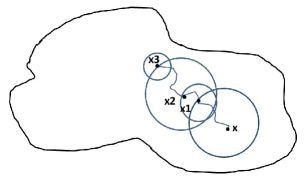
(a) WOS within the domain

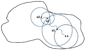
(b) WOS (with a maximal step size for each jump) within the domain

Figure 1: Walk on Spheres method

Next we define an estimator of (14) by

$$u(x)\approx\frac{1}{N}\sum_{i=1}^{N}u(x_{i}),$$ (23)

where $\displaystyle N$ is the number of Brownian paths sampled and $\displaystyle x_{i}$ is the first hitting point of each path on the boundary. Using a jump size (radius of the ball) $\displaystyle\delta$ on each step for the WOS, we expect to take $\displaystyle O(1/\delta^{2})$ steps for a Brownian path to reach the boundary [6]. To speed up, maximum possible size for each step would allow faster first hitting on the boundary. Most of the numerical results in this paper will use the WOS approach as illustrated in Figure 1(b).

5 Numerical Methods

5.1 Simulation of reflecting Brownian paths

A standard reflecting Brownian motion path can be constructed by reflecting a standard Brownian motion path back into the domain whenever it crosses the boundary. So in principle, the simulation of RBM is reduced to that of BM.

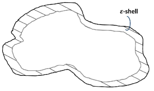
Figure 2: A $\displaystyle\epsilon$-region for a bounded domain in $\displaystyle R^{3}$

It is known that standard Brownian motion can also be constructed as the scaling limit of a random walk on a lattice so we can model BM by a random walk with proper scale (see Appendix for details). However, it turns out that the WOS method is the preferred method to simulate BM for our purpose [9] (see Remark 6 for details). As mentioned before, a $\displaystyle\epsilon$-shell is chosen around the boundary as the termination region in the Dirichlet case. Here we follow a similar strategy by setting up a $\displaystyle\epsilon$-region but allowing the process $\displaystyle X_{t}$ to continue moving after the latter reaches the $\displaystyle\epsilon$-region instead of being absorbed.

Figure 2 shows a strip region with width $\displaystyle\epsilon$ near the boundary is identified for a bounded domain. In a spherical domain, the $\displaystyle\epsilon$-region is simply an $\displaystyle\epsilon$-shell near the boundary of width $\displaystyle\epsilon$. Denote $\displaystyle M_{\epsilon}(D)$ as the $\displaystyle\epsilon$-region and $\displaystyle I(D)$ as the remaining interior region $\displaystyle D\backslash M_{\epsilon}(D)$.

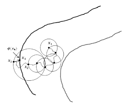
Figure 3: WOS in the $\displaystyle\epsilon$-region. BM path hits $\displaystyle x_{1}$ in $\displaystyle\epsilon$-region for the first time. Then the radius of sphere is changed to $\displaystyle\Delta x$, the path continues until it arrives at $\displaystyle x_{2}$ whose distance to $\displaystyle\partial D$ is smaller or equal to $\displaystyle\Delta x$. Then the radius of the ball is enlarged to 2$\displaystyle\Delta x$ so that the path has a chance to run out of the domain at $\displaystyle x_{3}$. If that happens, we pull back $\displaystyle x_{3}$ to $\displaystyle x_{4}$ which is the closest point to $\displaystyle x_{3}$ on the boundary. Record $\displaystyle\phi(x_{4})$, and continue WOS-sampling the path starting at $\displaystyle x_{4}$.

Recall the discussion of the WOS in the previous section. For a BM starting at a point $\displaystyle x$ in the domain, we draw a ball centered at $\displaystyle x$, the Brownian path will hit the spherical surface with a uniform probability as long as the ball does not overlap the domain boundary $\displaystyle\partial D$. The balls are constructed so that the jumps are as large as possible by taking the radius of the ball to be the distance to the boundary $\displaystyle\partial D$. We repeat this procedure until the path reaches the region $\displaystyle M_{\epsilon}(D)$. Here, we continue the WOS in $\displaystyle M_{\epsilon}(D)$ but with a fixed radius $\displaystyle\Delta x$ much smaller than $\displaystyle\epsilon$. In order to simulate the path of RBM, at some points of the time the BM path may run out of the domain. For this to happen, the radius of WOS is increased to $\displaystyle 2\Delta x$ when the path is close to boundary at a distance less than $\displaystyle\Delta x$. In this way, the BM path will have a chance to get out of the domain, and when that happens, we then pull it back to the nearest point on the boundary along the normal of the boundary. Afterwards, the BM path will continue as before.

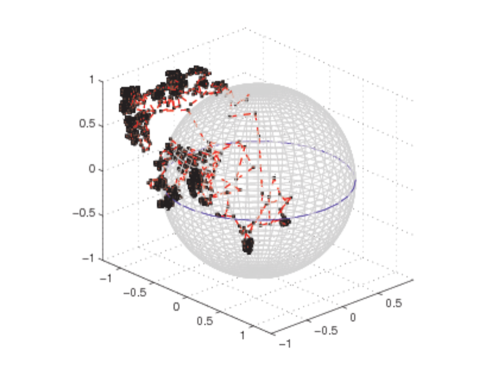
Figure 4: A RBM path with a cube in $\displaystyle R^{3}$

In summary, a reflecting Brownian motion path is simulated by the WOS method inside $\displaystyle D$. Once it enters the $\displaystyle\epsilon$-region $\displaystyle M_{\epsilon}(D)$, the radius of WOS changes to a fixed value, either $\displaystyle\Delta x$ or $\displaystyle 2\Delta x$, depending on its current distance of the Brownian particle to the boundary. Once the path reaches a point on the boundary after the reflection, the radius of WOS changes back to $\displaystyle\Delta x$. Figure 3 illustrates the movement of RBM in the $\displaystyle\epsilon$-region $\displaystyle M_{\epsilon}(D)$. As time progresses, we expect the path hits the boundary at some time instances and lies in either $\displaystyle I(D)$ or $\displaystyle M_{\epsilon}(D)$ at others. A RBM path is shown in Figure 4 within a cube of size 2.

5.2 Computing the boundary local time $\displaystyle L(t)$

Two equivalent forms of the local time have been given in (5) and (6). Here we will show how the $\displaystyle\epsilon$-region for the construction of the RBM in Fig. 3 can also be used for the calculation of the local time. When the $\displaystyle\epsilon$-region is thin enough, i.e. $\displaystyle\epsilon\ll 1$, an approximation of (5) is given in (10), which is the occupation time that RBM $\displaystyle X_{s}$ sojourns within the $\displaystyle\epsilon$-region during the time interval $\displaystyle[0,t]$. A close look at (10) reveals that only the time spent near the boundary is involved and the specific moment when the path enters the $\displaystyle\epsilon$-region has no effect on the calculation of $\displaystyle L(t)$.

Suppose $\displaystyle x\in D$ is the starting point of a Brownian path, which is simulated by the WOS method. Once the path enters the $\displaystyle\epsilon$-region, the radius of WOS is changed to $\displaystyle\Delta x$ or $\displaystyle 2\Delta x$. It is known that the elapsed time $\displaystyle\Delta t$ for a step of a random walk on average is proportional to the square of the step size, in fact, $\displaystyle\Delta t=(\Delta x)^{2}/d,d=3$ when $\displaystyle\Delta x$ is small (see Appendix), which also applies to WOS moves (See Remark 6 for details). Therefore, we can obtain an approximation of the local time $\displaystyle L(dt)$ by counting the number of steps the path spent inside $\displaystyle M_{\epsilon}(D)$ multiplied by the time elapsed for each step, i.e.

$$L(dt)=L(t_{j}-t_{j-1})\approx\frac{\int_{t_{j-1}}^{t_{j}}I_{D_{\epsilon}}(X_{s})ds}{\epsilon}=(n_{t_{j}}-n_{t_{j-1}})\frac{(\Delta x)^{2}}{3\epsilon},$$ (24)

where $\displaystyle n_{t_{j}}-n_{t_{j-1}}$ is the number of steps that WOS steps remain in the $\displaystyle\epsilon$-region during the time interval [$\displaystyle t_{j-1},t_{j}].$ Figure 5 gives a sample path of the simulated local time associated with the RBM in Figure 4.

Remark 5

(Alternative way to compute local time $\displaystyle L(t)$ ) From $\displaystyle(\ref{eq13})$, the local time increases if and only if the RBM path hits the boundary, which implies that the time before the path hits the boundary makes no contribution to the increment of the local time. Thus, a WOS method with a changing radius can also be used with $\displaystyle(\ref{eq13})$. Specifically, we divide the time interval $\displaystyle[0,t]$ into to $\displaystyle N$ small subintervals of equal length. In each $\displaystyle[t_{i},t_{i+1}]$ the Brownian path will move $\displaystyle 2\Delta x$ or $\displaystyle\Delta x$ with the WOS method when the current path lies within a distance less or more than $\displaystyle\Delta x$ to the boundary. If the path hits or crosses the boundary within $\displaystyle[t_{i},t_{i+1}]$, then $\displaystyle L(t)$ will increase by $\displaystyle\sqrt{\pi/2}\sqrt{t_{i+1}-t_{i}}$.

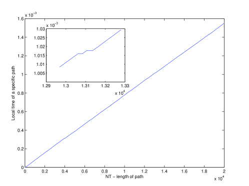
Figure 5: Boundary local time (24) increases when the path runs into the region $\displaystyle M_{\epsilon}(D)$. The insert shows the piecewise linear profile of the local time path with flat level regions. The path of $\displaystyle L(t)$ is a nondecreasing function and increases at a rate lower than $\displaystyle O(NT)$. $\displaystyle NT$ is the length of the path.

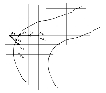
Figure 6: Random walks on the $\displaystyle\epsilon$-region. A BM path hits $\displaystyle x_{1}\in M_{\epsilon}(D)$ by the WOS method. Replace $\displaystyle x_{1}$ by the nearest grid point $\displaystyle x_{1}^{\prime}$. Then several steps of random walks will make a path as $\displaystyle x_{2}\rightarrow x_{3}\rightarrow x_{4}$. Since $\displaystyle x_{4}\notin D$, we push it back along the normal line (dash arrow) to $\displaystyle x_{4}^{\prime}$ then replace it by the closest grid point within domain (solid arrow) $\displaystyle x_{5}$. Here path crosses the boundary at $\displaystyle x_{4}^{\prime}\in\partial D$. Then continue the random walk as usual at $\displaystyle x_{6}$.

Remark 6

(Approximating RBM by WOS or random walks on a lattice - a comparison) There are two ways to find approximation to Brownian paths inside the region $\displaystyle M_{\epsilon}(D)$ and construct their reflections once they get out of the boundary. One way is by using the WOS approach as described in Section 5.1. The other is in fact to use a random walk on a lattice inside $\displaystyle M_{\epsilon}(D).$ In the second approach, as illustrated in Fig. 6, a grid mesh is set up over $\displaystyle M_{\epsilon}(D)$ and the random walk takes a one-step walk on the lattice until the path goes out of the domain and then it will be pushed back to the nearest lattice point inside $\displaystyle M_{\epsilon}(D)$. And the elapsed time for a $\displaystyle\Delta x$ walk is on average $\displaystyle(\Delta x)^{2}/3$ as shown in the Appendix. The boundary local time $\displaystyle L(t)$ can be still calculated as in $\displaystyle(\ref{eq45})$. The problem with this approach is that a Brownian motion actually should have equal probability to go in all directions in the space while a random walk on the lattice only considers six directions in $\displaystyle R^{3}$. This limitation was found in our numerical tests to lead to insufficient accuracy in simulating reflecting Brownian motions for our purpose.

Meanwhile, the WOS method in the $\displaystyle\epsilon$-region $\displaystyle M_{\epsilon}(D)$ has a fixed radius $\displaystyle\Delta x$, which enables us to calculate the boundary local time by $\displaystyle(\ref{eq45})$ since the elapsed time of a $\displaystyle\Delta x$ move in $\displaystyle R^{3}$ on average still remains to be $\displaystyle(\Delta x)^{2}/3$.  This conclusion can be heuristically justified by considering points on the sphere are the linear combination of the directions along the three axes, which implies that the average time that the path hits the sphere with radius $\displaystyle\Delta x$ should also be the same. As discussed before, if the path comes within a distance very close to the boundary, say less than $\displaystyle\Delta x$, the radius of the WOS method is increased to $\displaystyle 2\Delta x$ so that it will have a chance to run out of the domain and then be pushed back to the nearest point on the boundary to affect a hit of the RBM on the boundary.

5.3 Probabilistic representation for the Neumann problem

Finally, with the boundary local time of RBM available, we can come to the approximation of the Neumann problem solution $\displaystyle u(x)$ using the probabilistic approach (12). First of all, we will need to truncate the infinite time duration required for the RBM path $\displaystyle X_{t}$ in (12) to a finite extent for computer simulations. The exact length of truncation will have to be numerically determined by increasing the length until a convergence is confirmed (namely, the approximation to $\displaystyle u(x)$ does not improve within a prescribed error tolerance between two different choices of truncation times under same number of sampled paths). Assume that the time period is limited to from $\displaystyle 0$ to $\displaystyle T$, then by a Monte Carlo sampling of the RBM paths, an approximation of (12) will be

$$\widetilde{u}(x)=\frac{1}{2\epsilon}\sum_{i=1}^{N}\left[\int_{0}^{T}\phi(X_{t}^{i})I_{\partial D}(X_{t}^{i})\int_{t}^{t+dt}I_{D_{\epsilon}}(X_{s}^{i})ds\right],$$ (25)

where $\displaystyle X_{t}^{i},i=1,...,N$ are stochastic processes sampled according to the law of RBM.

Next, let us see how the RBM can be incorporated into the representation formula once its path is obtained.

Associate the time interval $\displaystyle[0,T]$ with the number of steps $\displaystyle NT$ of a sampling path, $\displaystyle NT$ will give the total length of each path. Then, the integral inside the square bracket in (25) can be transformed into $\displaystyle j$

$$\sum_{j^{\prime}=1}^{NT}\left(\phi(X_{t_{j}}^{i})I_{\partial D}(X_{t_{j}}^{i})\int_{t_{j-1}}^{t_{j}}I_{D_{\epsilon}}(X_{s}^{i})ds\right),$$ (26)

where $\displaystyle j^{\prime}$ stands for the $\displaystyle j^{\prime}-$th step the WOS method has taken, and $\displaystyle j$ indicates a step for which $\displaystyle X_{t_{j}}^{i}\in\partial D$.

As the integral in (26) is in fact the occupation time as shown in (24), (26) becomes

$$\sum_{j^{\prime}=1}^{NT}\left(\phi(X_{t_{j}}^{i})I_{\partial D}(X_{t_{j}}^{i})(n_{t_{j}}-n_{t_{j-1}})\frac{(\Delta x)^{2}}{3}\right).$$ (27)

As a result, an approximation to the PDE solution $\displaystyle\widetilde{u}(x)$ becomes

$$\widetilde{u}(x)=\frac{1}{2\epsilon}\sum_{i=1}^{N}\left[\sum_{j^{\prime}=1}^{NT}\left(\phi(X_{t_{j}}^{i})I_{\partial D}(X_{t_{j}}^{i})(n_{t_{j}}-n_{t_{j-1}})\frac{(\Delta x)^{2}}{3}\right)\right].$$ (28)

Theoretically speaking, $\displaystyle\epsilon$ should be chosen much larger than $\displaystyle\Delta x$. Here, we take $\displaystyle\epsilon=k\Delta x$, $\displaystyle k$ $\displaystyle>1$ is an integer, which will increase as $\displaystyle\Delta x$ vanishes to zero. Then, (28) reduces to

$$\widetilde{u}(x) =\frac{1}{2k\Delta x}\sum_{i=1}^{N}\left[\sum_{j=1}^{NT}\left(\phi(X_{t_{j}}^{i})I_{\partial D}(X_{t_{j}}^{i})(n_{t_{j}}-n_{t_{j-1}})\frac{(\Delta x)^{2}}{3}\right)\right]$$ (29)

$$=\frac{\Delta x}{6k}\sum_{i=1}^{N}\left[\sum_{j=1}^{NT}\left(\phi(X_{t_{j}}^{i})I_{\partial D}(X_{t_{j}}^{i})(n_{t_{j}}-n_{t_{j-1}})\right)\right],$$

which is the final numerical algorithm for the Neumann problem. In the following we present the general implementation of this numerical algorithm.

Let $\displaystyle x$ be any interior point in $\displaystyle D$ where the solution $\displaystyle u(x)$ for the Neumann problem is sought. First, we define the $\displaystyle\epsilon$-region $\displaystyle M_{\epsilon}(D)$ near the boundary. For each one of $\displaystyle N$ RBM paths, the following procedure will be executed until the length of the path reaches a prescribed length given by $\displaystyle NT\cdot\Delta x$:

1. If $\displaystyle x\notin M_{\epsilon}(D)$, predict next point of the path by the WOS with a maximum possible radius until the path locates near the boundary within a certain given distance $\displaystyle\epsilon,$ say $\displaystyle\epsilon=5\Delta x$ (hit the $\displaystyle\epsilon$-region $\displaystyle M_{\epsilon}(D)$). If $\displaystyle x\in M_{\epsilon}(D)$, $\displaystyle l(t_{i})=1$; otherwise, $\displaystyle l(t_{i})=0$. Here $\displaystyle l(t)$ is the unit increment of $\displaystyle L(t)$ at time $\displaystyle t$.

2. If $\displaystyle x\in M_{\epsilon}(D)$, use the WOS method with a fixed radius $\displaystyle\Delta x$ to predict the next location for Brownian path. Then, execute one of the two options:

Option 1. If the path happens to hit the domain boundary $\displaystyle\partial D$ at $\displaystyle x_{t_{i}}$, record $\displaystyle\phi(x_{t_{i}})$.

Option 2. If the path passes crosses the domain boundary $\displaystyle\partial D$, then pull the path back along the normal to the nearest point on the boundary. Record the Neumann value at the boundary location.

Due to the independence of the paths simulated with the Monte Carlo method, we can run a large number of paths simultaneously on a computer with many cores in a perfectly parallel manner, and then collect all the data at the end of the simulation to compute the average. Algorithm 1 gives a pseudo-code for the numerical realization of implementing the WOS in both $\displaystyle I(D)$ and $\displaystyle M_{\epsilon}(D)$ regions.

Data: Select integers $\displaystyle N$ and $\displaystyle NT$, a starting point $\displaystyle X_{0}\in D$, step size $\displaystyle h$ and $\displaystyle\epsilon$-region $\displaystyle M_{\epsilon}(D)$ near the boundary.

Output An approximation of $\displaystyle u(X_{0})$.

Initialization $\displaystyle L[NT],v[NT],u[N]$, $\displaystyle X=X_{0}$, $\displaystyle i\leftarrow 1$ and $\displaystyle j\leftarrow 1$;

While $\displaystyle i\leq N$ do

    Set $\displaystyle S_{i}=0$.

    While $\displaystyle j\leq NT$ do

       If $\displaystyle X\in I(D)$ then  /* If the path has not touched the $\displaystyle\epsilon$-region */

        Set $\displaystyle L[j]\leftarrow$ 0;  /*Increment of local time at each step. */

        Set $\displaystyle r\leftarrow d(X,\partial D)$; /* Find the distance to the boundary */

        Randomly choose a point $\displaystyle X_{1}$ on $\displaystyle B(X,r)$ then set $\displaystyle X\leftarrow X_{1}$.

       Else /* The path enters the $\displaystyle\epsilon$-region */

        $\displaystyle L[j]\leftarrow 1$;  /*local time increases */

        Set $\displaystyle r\leftarrow$ h (2h); /* If $\displaystyle d(X,\partial D)>h$ or =0 ($\displaystyle 0<d(X,\partial D)\leq h$) */

        Randomly choose a point $\displaystyle X_{1}$ on $\displaystyle B(X,r)$ then set $\displaystyle X\leftarrow X_{1}$.

        If $\displaystyle X\notin\bar{D}$, then

          Find $\displaystyle X_{j}$ to be the nearest point on $\displaystyle\partial D$ to X and pull $\displaystyle X$ back

          onto $\displaystyle\partial D$ at $\displaystyle X_{j}$;

          Set $\displaystyle X\leftarrow X_{j}$;

          Set $\displaystyle v[j]\leftarrow\phi(X_{j})$

        End

       End

       $\displaystyle j\leftarrow j+1$;

   End

    count $\displaystyle\leftarrow$ 0;

    For k=1:NT

       count $\displaystyle\leftarrow$ count + $\displaystyle L[k]$;

       If $\displaystyle v[k]\sim=0$ then

       $\displaystyle u[i]\leftarrow u[i]+\phi(X_{k})\cdot$count;

       count $\displaystyle\leftarrow$ 0;

    End

   $\displaystyle i\leftarrow i+1$;

End

Return $\displaystyle\widetilde{u}(X_{0})=h\sum_{k=1}^{N}u[k]/N/(6k)$

Algorithm 1: The algorithm for the probabilistic solution of the Laplace equation with the Neumann boundary condition

6 Numerical results

In this section, we give the numerical results for the Neumann problem in cubic, spherical and ellipsoid domains.

To monitor the accuracy of the numerical approximation of the solutions, we select a circle inside the domain, where the solution of the PDE $\displaystyle u(x)$ will be found by the proposed numerical methods, defined by

$$\{(x,y,z)^{T}=(r\cos\theta_{1}\sin\theta_{2},r\sin\theta_{1}\sin\theta_{2},r\cos\theta_{2})^{T}\}$$ (30)

with $\displaystyle r=0.6$, $\displaystyle\theta_{1}=0:k\cdot 2\pi/30:2\pi$, $\displaystyle\theta_{2}=\pi/4$ with $\displaystyle k=1,...,15$. In addition, a line segment will also be selected as the locations to monitor the numerical solution, the endpoints of the segment are $\displaystyle(0.4,0.4,0.6)^{T}$ and $\displaystyle(0.1,0,0)^{T}$, respectively. Fifteen uniformly spaced points on the circle or the line are chosen as the locations for computing the numerical solutions.

The true solution of the Neumann problem (1) with the corresponding Neumann boundary data is

$$u(x)=\sin 3x\sin 4y\ e^{5z}+5.$$ (31)

In the figures of numerical results given below, the blue curves are the true solutions and the red-circle ones are the approximations. The numerical solutions are shifted by a constant so they agree with the exact solution at one point as the Neumann problem is only unique up to an arbitrary additive constant. “Err”indicates the relative error of the approximations.

6.1 Cube domain and test on the length of the path

A cube domain of size 2 is selected to test the choice of the number of paths and the length of the paths (truncation time duration $\displaystyle T$) in the numerical formula (29).

The step-size $\displaystyle\Delta x=0.0005$ is used as the radius of the WOS inside the $\displaystyle\epsilon$-region $\displaystyle M_{\epsilon}(D)$, namely, the step-size of the random walk approximation of the RBM near the boundary. The number of paths is taken as $\displaystyle N=2e5.$ Two choices for the path length parameter $\displaystyle NP=2.7e4$ and $\displaystyle NP=3e4$ are compared to gauge the convergence of the numerical formula (29) in terms of the path truncation. Figures 7 and 8 shows the solution and the relative errors in both cases, which indicates that $\displaystyle NP=3e4$ will be sufficient to give an error around 5% as shown in Fig. 8.

In the rest of the numerical tests, we will set the number of path $\displaystyle N=2e5,$ and number of steps for each path $\displaystyle NP=3e4$.

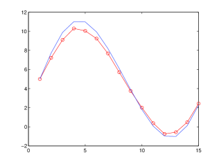
(a) $\displaystyle\epsilon$ = 6$\displaystyle\Delta x$, Err = 10.71%

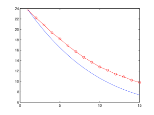
(b) $\displaystyle\epsilon$ = 7$\displaystyle\Delta x$, Err = 12.19%

Figure 7: Cubic domain: number of paths $\displaystyle N=2e5$, and number of steps for each path $\displaystyle NP=2.7e4$. (Left) Solution on the circle defined in (31), (right) solution on a line segment.

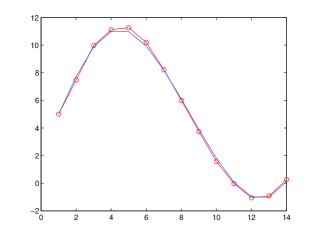
(a) $\displaystyle\epsilon$ = 6$\displaystyle\Delta x$, Err = 5.35%

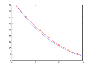
(b) $\displaystyle\epsilon$ = 7$\displaystyle\Delta x$, Err = 5.85%

Figure 8: Cubic domain: number of paths $\displaystyle N=2e5,$ and number of steps for each path $\displaystyle NP=3e4$. (Left) Solution on the circle defined in (31), (right) solution on a line segment.

6.2 Spherical domain

The unit ball is centered at the origin. We set $\displaystyle\Delta x=0.0005$ and adjust $\displaystyle\epsilon$, similar numerical results are obtained as in the case of the cube domain. Here, the reflected points of Brownian path are the intersection of the normal and the domain. Though Figure 8(b) shows some oscillations in the middle, the overall approximation are within a relative error around $\displaystyle 5.85\%$.

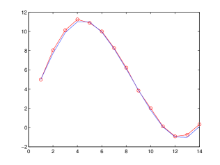
(a) $\displaystyle\epsilon$ = 5$\displaystyle\Delta x$, Err = 5.13%

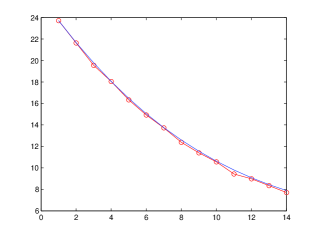
(b) $\displaystyle\epsilon$ = 5$\displaystyle\Delta x$, Err = 4.03%

Figure 9: Spherical domain: number of paths $\displaystyle N=2e5$, and number of steps for each path $\displaystyle NP=3e4$. (Left) Solution on the circle defined in (31), (right) solution on a line segment.

6.3 Ellipsoid domain

The ellipse with axis lengths $\displaystyle(3,\ 2,\ 1)$ is centered at the origin. We set $\displaystyle\Delta x=0.0004$. The numerical results along the circle behave better than those along the line segment, especially along the tail section of the latter (Figure 10(b)), which lie closer to the origin $\displaystyle\mathbf{0}$.

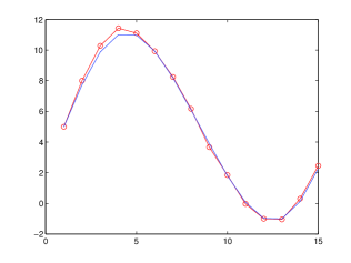
(a) $\displaystyle\epsilon$ = 5$\displaystyle\Delta x$, Err = 5.75%

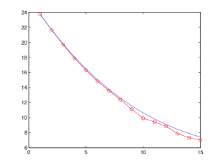
(b) $\displaystyle\epsilon$ = 5$\displaystyle\Delta x$, Err = 5.12%

Figure 10: Ellipsoid domain: number of paths $\displaystyle N=2e5$, and number of steps for each path $\displaystyle NP=3e4$. Left: solution on the circle defined in (31). Right: solution on a line segment.

7 Conclusions and discussion

In this paper we have proposed numerical methods for computing the local time of reflecting Brownian motion and the probabilistic solution of the Laplace equation with the Neumann boundary condition. Without knowing the complete trajectories of RBM in space, we are able to use the WOS to sample the RBM and calculate its local time, based on which a discrete probabilistic representation (29) was obtained to produce satisfactory approximations to the solution of the Neumann problem at one single point. Numerical results validated the stability and accuracy of the proposed numerical methods.

In addition, random walk on a lattice was also investigated as an alternative way to sample RBM. However, numerical experiments show that the numerical results are inferior to those obtained by the WOS method. A possible reason is that formula (5) for the local time is valid for a smooth path while a random walk approximation of the the Brownian path contains inherent errors.

The local time can also be computed by a mathematically equivalent formula (6), for which the implementation is discussed briefly in section 5.2. Again the numerical results based on (6) are inferior to those obtained using the original limiting process of Lévy in [3] . This fact we believe may result from the time discretization error of Brownian paths especially when long time truncation is employed in the probabilistic representation.

Various issues affecting the accuracy of the proposed numerical methods remain to be further investigated, such as the number of random walk or WOS steps and the truncation of duration time $\displaystyle T$ for the paths, the choice of the thickness for the $\displaystyle\epsilon$-region, the size of $\displaystyle\Delta x$ for the lattice, etc. In theory, the larger the truncation time $\displaystyle T$, the more accurate is the probabilistic formula for the Neumann solution. However, for a fixed spatial mesh size $\displaystyle\Delta x,$ long time integration will result in the accumulation of time discretization error for the Brownian pathes, thus leading to the degeneracy of the numerical solutions as verified by our numerical experiments. Meanwhile, Révész [18] have proposed some approximations of local time by other stochastic processes in the case of a half line. We conjecture such results may still hold in higher dimensions and progress in this direction will shed light on how to improve the numerical procedures proposed in this paper.

8 Appendix

If the random walk on a lattice as in Fig. 11 is to converge to a continuous BM, a relationship between $\displaystyle\Delta t$ and $\displaystyle\Delta x$ in $\displaystyle R^{3}$ will be needed and is shown to be

$$\Delta t=\frac{(\Delta x)^{2}}{3}.$$ (32)

The following is a proof for this result (See [12] for reference). The density function of standard BM satisfies the following PDE [1]

$$\frac{\partial p}{\partial t}=\frac{1}{2}\Delta_{x}p(t,x,y)\ .$$ (33)

By using a central difference scheme and changing $\displaystyle p$ to $\displaystyle v$, equation (33) becomes

$$\frac{v_{i,j,k}^{n+1}-v_{i,j,k}^{n}}{\Delta t}=\frac{1}{2}\frac{v_{i+1,j,k}^{n}+v_{i-1,j,k}^{n}+v_{i,j+1,k}^{n}+v_{i,j-1,k}^{n}+v_{i,j,k+1}^{n}+v_{i,j,k-1}^{n}-6v_{i,j,k}^{n}}{(\Delta x)^{2}}\text{ }.$$ (34)

Reorganizing and letting $\displaystyle\lambda=\Delta t/(2(\Delta x)^{2})$ , we have

$$v_{i,j,k}^{n+1}=\lambda v_{i+1,j,k}^{n}+\lambda v_{i-1,j,k}^{n}+\lambda v_{i,j+1,k}^{n}+\lambda v_{i,j-1,k}^{n}+\lambda v_{i,j,k+1}^{n}+\lambda v_{i,j,k-1}^{n}+(1-6\lambda)v_{i,j,k}^{n}\text{ },$$ (35)

By setting $\displaystyle\lambda=\frac{1}{6}$, we have

$$v_{i,j,k}^{n+1}=\frac{1}{6}v_{i+1,j,k}^{n}+\frac{1}{6}v_{i-1,j,k}^{n}+\frac{1}{6}v_{i,j+1,k}^{n}+\frac{1}{6}v_{i,j-1,k}^{n}+\frac{1}{6}v_{i,j,k+1}^{n}+\frac{1}{6}v_{i,j,k-1}^{n}.$$ (36)

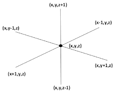
Figure 11: Central difference scheme in $\displaystyle R^{3}$

For the initial condition $\displaystyle\phi$, we have

$$v_{i,j,k}^{n+1}=\sum_{i^{\prime},j^{\prime},k^{\prime}}C_{i^{\prime},j^{\prime},k^{\prime}}\phi\left(\sum_{l=1}^{n}\overset{\rightarrow}{\eta_{l}}\right)$$ (37)

where

$$\overset{\rightarrow}{\eta_{l}}=\left\{\begin{aligned} &(-h,0,0)^{T},\ &prob=\frac{1}{6}\\ &(h,0,0)^{T},\ &prob=\frac{1}{6}\\ &(0,h,0)^{T},\ &prob=\frac{1}{6}\\ &(0,-h,0)^{T},\ &prob=\frac{1}{6}\\ &(0,0,h)^{T},\ &prob=\frac{1}{6}\\ &(0,0,-h)^{T},\ &prob=\frac{1}{6}\\ \end{aligned}\right.,$$ (38)

and

$$\sum_{l=1}^{n}\overset{\rightarrow}{\eta_{l}}=\left(\begin{aligned} &-n+2i^{\prime}+i\\ &-n+2j^{\prime}+j\\ &-n+2k^{\prime}+k\\ \end{aligned}\right)h.$$ (39)

Let $\displaystyle\overset{\rightarrow}{\eta_{l}}=(x_{l},y_{l},z_{l})^{T}$, then

$$x_{l}=\left\{\begin{aligned} -h,\ &prob=\frac{1}{6}\\ h,\ &prob=\frac{1}{6}\\ 0,\ &prob=\frac{2}{3}\\ \end{aligned}\right.,$$ (40)

for each $\displaystyle l$. We known that $\displaystyle y_{l}$, $\displaystyle z_{l}$ have the same distribution as $\displaystyle x_{l}$.

Notice that the covariance between any two of $\displaystyle x_{l}$, $\displaystyle y_{l}$, $\displaystyle z_{l}$ is zero, i.e. $\displaystyle E(x_{l}y_{l})=0$, $\displaystyle E(y_{l}z_{l})=0$ and $\displaystyle E(x_{l}z_{l})=0$. So $\displaystyle E(\sum_{i=1}^{n}x_{l}\sum_{i=1}^{n}y_{l})=0$, $\displaystyle E(\sum_{i=1}^{n}y_{l}\sum_{i=1}^{n}z_{l})=0$ and $\displaystyle E(\sum_{i=1}^{n}x_{l}\sum_{i=1}^{n}z_{l})=0$. According to the central limit theorem, we have

$$\sum_{i=1}^{n}x_{l}\overset{D}{=}N\left(0,\frac{nh^{2}}{3}\right)\ as\ \ n\rightarrow\infty.$$ (41)

The same assertion holds for $\displaystyle\sum_{i=1}^{n}y_{l}$ and $\displaystyle\sum_{i=1}^{n}z_{l}$.

Since $\displaystyle\lambda=\frac{\Delta t}{2(\Delta x)^{2}}=\frac{1}{6}$, then $\displaystyle h^{2}=3k$ and hence $\displaystyle\frac{nh^{2}}{3}=nk=t$. Therefore $\displaystyle\sum_{i=1}^{n}x_{l}\ \sim N(0,t)$ as $\displaystyle n\rightarrow\infty$. So are $\displaystyle\sum_{i=1}^{n}y_{l}$ and $\displaystyle\sum_{i=1}^{n}z_{l}$.

Recall that the covariance between any pair of $\displaystyle\sum_{i=1}^{n}x_{l}$, $\displaystyle\sum_{i=1}^{n}y_{l}$, and $\displaystyle\sum_{i=1}^{n}z_{l}$ is zero, that $\displaystyle\sum_{i=1}^{n}x_{l}$,$\displaystyle\sum_{i=1}^{n}y_{l}$ and $\displaystyle\sum_{i=1}^{n}z_{l}$ are independent normal random variables. Hence,

$$C_{i^{\prime},j^{\prime},k^{\prime},n}=P\left\{\sum_{l=1}^{n}\overset{\rightarrow}{\eta_{l}}=\left(\begin{aligned} &-n+2i^{\prime}+i\\ &-n+2j^{\prime}+j\\ &-n+2k^{\prime}+k\\ \end{aligned}\right)h=\left(\begin{aligned} \sum_{i=1}^{n}x_{l}\\ \sum_{i=1}^{n}y_{l}\\ \sum_{i=1}^{n}z_{l}\\ \end{aligned}\right)\right\}\overset{D}{\rightarrow}\frac{1}{(2\pi t)^{3/2}}e^{\frac{-\|\overset{\rightarrow}{x}-\overset{\rightarrow}{x_{0}}\|^{2}}{2t}},$$ (42)

and

$$v_{i,j,k}^{n+1}=\sum_{i^{\prime},j^{\prime},k^{\prime}}C_{i^{\prime},j^{\prime},k^{\prime},n}\phi(\sum_{l=1}^{n}\overset{\rightarrow}{\eta_{l}})\rightarrow\iiint_{R^{3}}\frac{1}{(2\pi t)^{3/2}}e^{\frac{-\|\overset{\rightarrow}{x}-\overset{\rightarrow}{x_{0}}\|^{2}}{2t}}\phi(\overset{\rightarrow}{x})d\overset{\rightarrow}{x},$$ (43)

which coincides with the density function of the 3-$\displaystyle d$ standard BM.

In conclusion, when $\displaystyle\frac{\Delta t}{2(\Delta x)^{2}}=\frac{1}{6}$, i.e. $\displaystyle\Delta t=\frac{(\Delta x)^{2}}{3}$ or $\displaystyle\sqrt{dt}=\frac{dx}{\sqrt{3}}$, the central difference scheme converges to the standard BM in 3-$\displaystyle d$. Generally, the result can be extended to $\displaystyle d$-dimensional Euclidean space and the result will be $\displaystyle\Delta t=\frac{(\Delta x)^{2}}{d}$.

References

- [1] (Elton) P. Hsu, ”Reflecting Brownian motion, boundary local time and the Neumann problem”, Dissertation Abstracts International Part B: Science and Engineering[DISS. ABST. INT. PT. B- SCI. ENG.], Vol. 45, No. 6, 1984.
- [2] G. A. Brosamler, A probabilistic solution of the Neumann problem, Mathematica Scandinavica, Vol. 38, 137-147, 1976.
- [3] P. Lévy, Pocessus Stochastiques et Mouvement Brownien, Gauthier-Villars, Paris, 1948.
- [4] C. Yan, W. Cai and X. Zeng, A parallel method for solving Laplace equations with Dirichlet data using local boundary integral equations and random walks, SIAM J. Scientific Computing, Vol. 35, No. 4, B868- B889, 2013.
- [5] J. A. Given, Chi-Ok Hwang and M. Mascagni, First- and last-passage Monte Carlo algorithms for the charge density distribution on a conducting surface, Physical Review E 66, 056704, 2002.
- [6] I. Binder and M. Braverman, The rate of convergence of the walk of sphere algorithm, Geometric and Functional Analysis, Vol. 22, 558-587, 2012.
- [7] M.E. Müller, Some continuous Monte Carlo methods for the Dirichlet problem, The Annals of Mathematical Statistics, Vol. 27, No. 3, 569-589, 1956.
- [8] J.-P. Morillon, Numerical solutions of linear mixed boundary value problems using stochastic representations, Int. J. Numer. Meth. Engng., Vol. 40, 387-405, 1997.
- [9] K. K. Sabelfeld and N. A. Simonov, Random walks on boundary for solving PDEs, Walter de Gruyter, 1994.
- [10] F. C. Klebaner, Introduction to Stochastic Calculus with Applications, Imperial College Press, 2001.
- [11] P. Mörters and Y. Peres, Brownian motion, Cambridge University Press, Vol. 30, 2010.
- [12] A. J. Chorin and O. H. Hald, Stochastic tools in mathematics and science, Dordrecht: Springer, Vol. 1, 2009.
- [13] I. Karatzas and S. E. Shreve, Brownian motion and stochastic calculus, Springer-Verlag New York Inc., 1988.
- [14] K. L. Chung and R. J. Williams, Introduction to Stochastic Integration, Progress in Probability and Statistics, Vol. 4, 1983.
- [15] J.E. Souza de Cursi, Numerical methods for linear boundary value problems based on Feynman-Kac representations, Mathematics and computers in simulation, Vol. 36, No. 1, 1-16, 1994.
- [16] M. Freidlin, Functional Integration and Partial Differential Equations, Princeton University Press, 1985.
- [17] A. Friedman, Stochastic differential equations and applications, Dover publication, 2006.
- [18] M. Csörgő and P. Révész , Three Strong Approximation of The Local Time of a Wiener Process and Their Applications to Invariance, North-Holland, 1984.
- [19] F. Fogolari, A. Brigo and H. Molinari, The Boltzmann equation for biomolecular electrostatics: a tool for structural biology, J. Mol. Recognit., Vol. 15, 377- 392, 2002.