The GBT 67 – 93.6 GHz Spectral Line Survey of Orion-KL

Abstract

We present a 67–93.6 GHz spectral line survey of Orion-KL with the new 4 mm Receiver on the Green Bank Telescope (GBT). The survey reaches unprecedented depths and covers the low-frequency end of the 3 mm atmospheric window which has been relatively unexplored previously. The entire spectral-line survey is published electronically for general use by the astronomical community. The calibration and performance of 4 mm Receiver on the GBT is also summarized.

1 Introduction

The Orion Nebula, the nearest region containing high-mass star formation (at a distance of only 414 pc, Menten et al. 2007), is one of the most studied objects in the entire sky. Within the Orion Molecular Cloud 1 (OMC1) complex, the Kleinmann-Low (KL) nebular harbors one of the most luminous embedded infrared sources (Wynn-Williams et al. 1984). The hot core and the intense shocks associated with the ongoing star formation within the massive molecular cloud give rise to very rich and complex chemistry (e.g., Esplugues et al. 2014).

Orion has been an important target of several spectral-line surveys (e.g., Sutton et al. 1985; Turner 1989; Lee et al. 2001; Schilke et al. 1997, 2001; Lee & Cho 2002; Lerate et al. 2006; Olofsson, A. et al. 2007; Carter et al. 2012), as spectral-line observations are key to disentangling the chemistry and physical processes in star-forming regions. Spectral surveys at 1 mm and shorter wavelengths are complicated by line confusion. Within the 3 mm atmospheric window, astronomical line confusion is less of an issue, and the window contains the fundamental ground-state transitions of several key molecular species.

The 4 mm Receiver was commissioned on the Robert C. Byrd Green Bank Telescope (GBT) in 2012. In this paper, we present the 67–93.6 GHz spectral line survey of Orion-KL taken with the new instrument.

2 The 4 mm Receiver

The 4 mm Receiver is a dual-beam, corrugated feed horn receiver that covers the frequency range of approximately 67–93 GHz. The system is a single-side band receiver, and both feeds are within the cold cryostat (15 K). The first version of the 4 mm Receiver (White et al. 2012) used a modified version of the W-band low-noise amplifiers (LNAs) originally built for the Wilkinson Microwave Anisotropy Probe (Pospieszalski et al. 2000). This receiver exhibited noise temperatures better than 80 K over much of the frequency band and was used during the initial observing season (through the summer of 2012). In the fall of 2012, the receiver was upgraded with LNAs developed for this band with more modern InP high-electron-mobility transistor (HEMT) devices (Pospieszalski 2012, Bryerton at al. 2013). The upgraded amplifiers reduced the receiver noise to 40 K over much of the band.

Unlike other receivers on the GBT, there are no noise diodes for calibration with the 4 mm Receiver. The receiver has an optical wheel external to the cryostat that is used for calibration. The wheel also contains a quarter-wave plate for the conversion of linear polarization into circular polarization for very long baseline interferometry (VLBI) observations. For calibration, the wheel has an ambient temperature load ($T_{\rm amb}$ that is monitored by a sensor) and an offset mirror used to view an internal cold load that has a stable effective temperature ($T_{\rm cold}$), which is derived from laboratory measurements. For calibration, the table is rotated to place the cold and ambient loads into each of the beams with alternating observations. Using the known temperatures of the loads, the effective gains ($g$ [Kelvin/Volt]) of the system are measured.

3 Observations

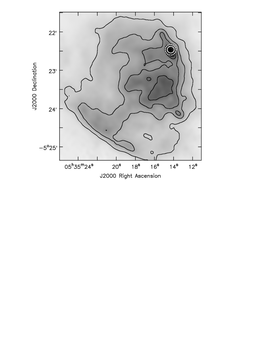
Figure 1: The GBT Mustang 90 GHz continuum image of Orion shown as grey-scale and contours (Dicker et al. 2009). The contours start at 0.2 Jy and are incremented by 0.2 Jy. The location of the nominal GBT beam at 77 GHz of the spectral-line observations is shown by the solid white circle, which corresponds to the bright continuum position of Orion-KL. The dotted white circle shows the possible area observed including the pointing errors and the variation of the beam size during the daytime observations.

Orion-KL was observed using the 4 mm Receiver on the GBT (project GBT12A_364) during four observational sessions between 2012 May 30 and 2012 June 15. The observed position of Orion-KL was $\alpha{\rm(J2000.0)}=05^{\rm h}35^{\rm m}14\fs 28$, $\delta{\rm(J2000.0)}=-05\arcdeg 22\arcmin 27\farcs 5$, corresponding to the bright continuum peak (Fig. 1). We adopt a source LSR velocity of $V_{LSR}=8.8\,\textstyle\rm{km~{}s}^{-1}$ (Turner 1989). The observations were taken in position-switched mode with alternating 1 minute ON and 1 minute OFF scans, using beam-1 of the receiver with both linear polarization channels. The OFF position was offset by one degree in right ascension and at the same declination as Orion-KL.

Twelve individual setups using the wide-bandwidth mode of the GBT Spectrometer (see GBT proposer’s guide) were used to carry out the survey with a channel resolution of 0.39 MHz ($\sim 1.5\,\textstyle\rm{km~{}s}^{-1}$). In total, 38 overlapping 800 MHz spectrometer windows separated by 700 MHz were used to cover the full frequency range of 67.0 GHz to 93.6 GHz. For each frequency set up, a sequence of 10 ON-OFF pairs of Orion-KL observations were carried out along with short calibration scans of the cold and ambient loads before and after the target observations. The observations for each setup were repeated twice, resulting in a nominal total integration time of 20 minutes of on-source data per frequency (20 ON-OFF pairs).

Observations of Jupiter and the nearby quasar 0423$-$0120 were used to derive pointing and focus corrections every hour. Representative daytime pointing offsets during the observing sessions were $2\farcs 7\pm 2\farcs 1$ which is a smaller than the 10-13$\arcsec$ beam and much smaller than the Orion complex which shows strong emission over 1-3 arc-minutes.

Given the extended source size, most of the observations were done without the “AutoOOF” measurements that are used to provide the thermal corrections to the active surface (see GBT documentation for a description of AutoOOF). In contrast, optimal point-source observations should be carried out with regular AutoOOF measurements during the nighttime when the thermal stability of the dish is best. Based on commissioning tests with the 4 mm Receiver, the AutoOOF corrections improve the point-source aperture efficiency by 30% or more. Application of these corrections during the day are not typically practical for the 4 mm Receiver given that the thermal environment of the dish is generally not sufficiently stable. During the day, the measured beam size was found to vary significantly (e.g., 10–$13\arcsec$), but the beam shape remained well-behaved (fairly symmetric and Gaussian). Although the variation of beam size has a direct impact on the point-source aperture efficiency ($\eta_{a}$), it has little impact on the effective main-beam efficiency ($\eta_{mb}$) used for the calibration of extended sources. For example during the commissioning of the instrument, we measured a beam size of $10\farcs 8$ at 77 GHz and derived $\eta_{a}=31$% and $\eta_{mb}=50$% in good nighttime conditions with the application of the thermal AutoOOF surface corrections. Without the AutoOOF corrections, the beam-size increased to 12$\farcs 5$ and the aperture efficiency decreased to 23%, but the main-beam efficiency remained nearly constant at about 50%. Given the insensitivity of $\eta_{mb}$ for extended source emission, we adopt the main-beam temperature scale $T_{mb}$ for the calibration of the data.

The main-beam temperature $T_{mb}$ is computed from the observed antenna temperature $T_{A}$ using the relationship

$$T_{mb}=T_{A}\exp(\tau_{o}A)/\eta_{mb},$$ (1)

where $\tau_{o}$ is the zenith opacity, $A$ is the airmass, and $\eta_{mb}$ is the main-beam efficiency. The opacity is derived from the weather database for Green Bank which successfully forecasts the opacity as a function of frequency and time with an accuracy of $\Delta(\tau)=0.006$ (Maddalena 2010a). For the four observational sessions, the zenith opacity varied only slightly ($\Delta\tau\simeq 0.02$–0.03). The opacity variations contribute less than 3% to the total error budget of $T_{mb}$.

The antenna temperature for each ON-OFF scan pair is given by

$$T_{A}=T_{\rm sys}(V_{ON}-V_{OFF})/V_{OFF},$$ (2)

where $T_{\rm sys}$ is the single-side-band system temperature and $V_{ON}$ and $V_{OFF}$ are the measured voltages of the ON and OFF scans. The calibration scans are used to measure the gain ($g$) and compute the system temperature for the OFF scan ($T_{\rm sys}=g\,V_{OFF}$). Based on the known temperatures ($T$) and measured voltages ($V$) of the ambient ($amb$) and cold loads, the gain is given by

$$g=[(T_{amb}-T_{cold})/(V_{amb}-V_{cold})].$$ (3)

We adopt the median value of $T_{\rm sys}$ across each spectral window in calibrating the spectra using equation (2). This is referred to “scalar” calibration within GBT documentation and contrasts to “vector” calibration which uses $T_{\rm sys}$ computed as a function frequency. Currently for the 800 MHz spectral windows, scalar calibration gives significantly better baseline performance than vector calibration for the 4 mm Receiver.

Assuming a Gaussian beam, the main-beam efficiency is given by

$$\eta_{mb}=0.8899\eta_{a}(\theta_{FWHM}D/\lambda)^{2},$$ (4)

where $\eta_{a}$ is the aperture efficiency, $\theta_{FWHM}$ is the full-width half-maximum beam size in radians, D is the diameter of the GBT (100m), and $\lambda$ is the observed wavelength (Maddalena 2010b). The applicability of this equation was confirmed directly by integrating the intensity profiles taken during the pointing scans. Based on measurements as a function of frequency, $\theta_{FWHM}\simeq 10\farcs 8({\rm 77\,GHz}/\nu)$, where $\nu$ is the frequency in GHz.

Observations of 3C279 in 2012 March were used to measure the aperture efficiency. For the GBT, $\eta_{a}=0.352T_{A}\exp(\tau_{o}A)/S_{\nu}$. Based on available measurements from the Atacama Large Millimeter Array (ALMA) and the Combined Array for Research Millimeter-wave Astronomy (CARMA), the derived flux density for 3C279 at the time of the GBT observations was $S_{\nu}{(\rm 77\,GHz)}=23\pm 2$ Jy. The corresponding derived aperture efficiency at 77 GHz is $31\pm 4$%. This efficiency is consistent with net surface errors of $\epsilon=280\mu\rm{m}$ using the Ruze equation:

$$\eta_{a}=0.71\exp[-(4\pi\epsilon/\lambda)^{2})],$$ (5)

where the coefficient 0.71 is the aperture efficiency at long wavelengths for the GBT. Adopting $\epsilon=280\mu\rm{m}$, equation (5) was used to compute $\eta_{a}$ as a function of wavelength.

The calibration results based on 3C279 at 77 GHz were confirmed within measurement errors with additional observations of Mars at 77 GHz (2012 March), 3C84 at 89 GHz (2013 December), and 0927+392 at 89 GHz (2013 March). In terms of absolute flux calibration, there is some degeneracy between the uncertainty of the temperature of the cold load and the derived aperature efficiency, and hence $T_{mb}$. The effective temperature of the the cold load derived in the lab is known to within 10%, which corresponds to a 2.5% uncertainty in $T_{mb}$. The uncertainty in the cold load contributes negligibly to the total error budget in comparison to the measurement errors of the astronomical observations. Factoring all known sources of errors, the estimated uncertainty on the calibrated $T_{mb}$ temperature scale is 17%.

4 Results

The observational parameters as a function of frequency are given in Table 1. The measured system temperature, aperture efficiency, and main-beam efficiency are shown in Figure 2. After data editing, removing a low-order polynomial baseline, and combining the data for both polarizations and observing sessions, the resulting empirical noise level per 0.39 MHz channel is 20–40 mK over most of the frequency range. The 38 calibrated overlapping spectrometer windows were spliced together to form a data set comprising of 68,096 frequencies and $T_{mb}$ values (Table 2). The complete tabulated data set is available as supplemental online material from the journal. Figure 3 displays the entire data set ploted on a logrithmic scale. To show the typical noise properties and baseline quality of the data, an example portion of the survey is plotted as Figure 4. Overlapping spectra separated by 0.5 GHz for the entire survey are provided in the supplemental online material (Fig. 5).

The data are fairly clean, but a few artifacts remain in the data from atmospheric O₂ and radio-frequency interference (RFI). Table 3 lists the frequency of data features that are not associated with Orion-KL. The “P-Cygni” profiles from O₂ result from position-switching. Separate frequency-switched observations were carried out to verify the association of these features with broad atmospheric O₂ lines.

The detected spectral lines were fitted with a Gaussian using the GBTIDL fitgauss routine. Below 1 K the data are very rich, and the identifications of weak features become challenging in many cases due to blended transitions and the associated with multiple possible species. In Table 4, we provide the results of fitting the brightest features ($T_{mb}>1$ K). In total, we tabulate measurements for 140 lines brighter than 1 K. These measurements represent only a small fraction of 727 spectral features detected in the data. The species associate with each of the lines in Table 4 were identified using the spectral line catalogs given within Splatalogue which is based on several spectroscoptic databases (Müller et al. 2005; Prickett et al. 1998; Lovas & Dragoset 2004). For each line, we list the most likely species. For the bright lines listed in Table 4, only one feature was not identified. This transition was measured at $T_{mb}=3.9$ K at an observed frequency of 81.756 GHz. Species with cataloged transitions closest in the frequency to this unidentified line include c-HCOOH (formic acid), H₂NCH₂CN (aminoacetonitrile), CH₃COCH₃ (acetone), and CH₂ND, but none of these possible identifications seem particularly compelling due to significant velocity offsets or the lack of other detected transitions associated with the species.

The vast majority of the spectral lines detected are associated with the cooler molecular gas regions consistent with velocities of $v_{\rm LSR}=8.8\,\textstyle\rm{km~{}s}^{-1}$ and widths of about $5\,\textstyle\rm{km~{}s}^{-1}$, or with the “hot core” region with $v_{\rm LSR}\approx 5\,\textstyle\rm{km~{}s}^{-1}$ and widths of about $10\,\textstyle\rm{km~{}s}^{-1}$ (Sutton et al. 1985). The SO₂ features show an additional broad component that may be associated with a strong outflow in the system (e.g., Wright et al. 1996).

The spectral lines observed with the 100-meter GBT are typically a few to more than 10 times brighter than those previously measured by the much smaller NRAO 36 Foot telescope (Turner 1989), and the brightest lines (e.g., SiO and HCN) observed with the GBT also tend to be brighter than those observed with the IRAM 30m (Carter et al. 2012). The variations in line strengths from different telescopes highlight the effects of beam dilution and filling factor effects where the observed intensity from small emission regions decreases with an increasing telescope beam size. However, many species also show good agreement in their observed line strengths. We find similar line strengths within measurement errors between the tabulated 30m measurements (Esplugues et al. 2013; Tercero et al. 2010) and those presented in Table 4 from the GBT for the SO, ³⁴SO, SO₂, and OCS transitions. These results suggest that the emission from these species are extended over both the 30m and GBT beams. The interpretation of line strengths is also complicated due to the multiple overlapping components of the Orion complex (extended ridge, compact ridge, plateau, and hot core; e.g., Tercero et al. 2010). Telescopes with different beam sizes will not observe the exact same portion of the Orion complex in a single pointing. High-spatial resolution mapping observations would be useful in disentangling the relative line strengths from the different components in Orion given that the components also have similar velocities (e.g., Widicus Weaver & Friedel 2012; Brouillet et al. 2013).

5 Concluding Remarks

In this paper we present the 67–93.6 GHz spectral-line survey of Orion-KL taken with the GBT. The full spectrum is available electronically. We tabulate spectral-line measurements for features brighter than $T_{mb}>1$ K, but features as weak as 10 mK are identifiable in the data. The survey targeted the bright continuum peak of Orion-KL. Many molecules are known to have strong emission elsewhere within Orion (e.g., Peng et al. 2013), and the GBT beam of $10\arcsec$ would be well-suited for mapping the distribution of molecular emission throughout the Orion complex.

Given the large collecting area of the GBT, the improved accuracy of the surface, and the excellent performance of the optimized LNAs, the GBT 4 mm system is the most sensitive facility in the world for this band. Within the over-lapping frequency range of ALMA band-3, the GBT system can achieve better system temperatures in spite of the higher opacity associated with the lower elevation of the Green Bank site. With the multi-pixel instruments currently under development (e.g., Argus, Sieth et al. 2014; Mustang-2, Dicker et al. 2014), the mapping speed within this band using the GBT would be unparalleled.

Figure 2: The measured system temperatures for the Orion-KL data are shown by squares (2012 June), and the improved system temperatures with the upgraded cold amplifies are shown by triangles (2012 December). Both data sets were taken in similar atmospheric opacity. The telescope efficiency scale is shown to the right. The measured main-beam efficiency ($\eta_{mb}$) and aperture efficiency ($\eta_{a}$) are shown as a function of frequency by the solid and dotted lines, respectively.

Figure 3: The 67–93.6 GHz spectrum of Orion-KL taken with the GBT. The data have been baseline subtracted, but the spectrum has been shifted by $+1$ K for plotting on a logarithm scale.

Figure 4: An example portion of the survey that includes the strong HCN(1-0) emission line. The top panel shows the full data range, while the bottom panel shows the same data zoomed-in along the y-axis to highlight the visibility of weak features. Spectral features are marked by the dotted-lines and labeled by species. The dotted-lines of neighboring transitions from the same species are connected by a solid line below the spectrum for clarity. The feature labeled with a “U” is unidentified. The full survey plotted similarly with overlapping spectra separated by 0.5 GHz is provided as supplemental online material (Fig. 5).

Table 1: Observational Parameters

Frequency	T(on)	$T({\rm sys})$	$\eta_{mb}$	$\sigma$
GHz	min	K		mK
(1)	(2)	(3)	(4)	(5)
67.35	24.55	314	0.61	77.0
68.05	17.85	277	0.60	61.7
68.75	19.80	256	0.60	71.2
69.45	19.80	216	0.59	43.9
70.15	19.80	201	0.58	36.7
70.85	20.75	181	0.57	33.0
71.55	20.80	172	0.56	32.0
72.25	20.80	174	0.56	28.4
72.95	20.80	165	0.55	33.5
73.65	19.60	180	0.54	33.9
74.35	19.80	146	0.53	26.8
75.05	19.80	155	0.53	29.5
75.75	19.80	143	0.52	26.9
76.45	19.80	147	0.51	32.5
77.15	18.80	134	0.50	27.6
77.85	18.80	128	0.50	25.0
78.55	18.80	143	0.49	30.9
79.25	18.80	140	0.48	31.3
79.95	19.80	129	0.47	24.6
80.65	19.80	126	0.47	22.6
81.35	19.80	130	0.46	26.7
82.05	19.90	142	0.45	33.0
82.75	18.80	154	0.45	40.8
83.45	18.80	155	0.44	31.9
84.15	18.80	156	0.43	33.0
84.85	18.80	154	0.42	39.4
85.55	19.80	177	0.42	36.9
86.25	19.80	172	0.41	45.9
86.95	19.80	197	0.40	43.9
87.65	19.80	185	0.40	38.5
88.35	19.80	167	0.39	37.9
89.05	19.80	145	0.38	38.2
89.75	19.80	129	0.38	31.9
90.45	19.80	149	0.37	36.1
91.15	19.80	128	0.36	45.3
91.85	19.80	157	0.36	50.2
92.55	19.80	175	0.35	59.2
93.25	19.65	159	0.34	52.3

Table 2: The GBT 67 – 93.6 GHz Spectrum of Orion-KL

LSR Frequency	$T_{mb}$
GHz	K
(1)	(2)
66.998244	-0.008832
66.998634	0.123508
66.999025	0.079210
66.999416	0.023435
66.999806	-0.065857
67.000197	0.092554

Table 3: Data Artifacts

Frequency	Feature
GHz
67.370	Atmospheric O2
67.901	Atmospheric O2
68.431	Atmospheric O2
82.495	RFI
82.851	RFI
86.629	RFI

Table 4: Bright Line Measurements and Identification

Frequency	Line Peak	FWHM	Identified Species
MHz	K	MHz
(1)	(2)	(3)	(4)
67847.503$\pm$0.074	1.30$\pm$0.09	2.11$\pm$0.23	SO2
68303.919$\pm$ 0.035	4.68$\pm$0.41	0.78$\pm$0.08	CH3OH
68553.163$\pm$0.033	1.10$\pm$0.09	0.83$\pm$0.08	CH3OH
68970.754$\pm$0.075	19.20$\pm$0.71	3.65$\pm$0.24	SO2

References

- (1) Brouillet, N., et al. 2013, A&A, 550, A46
- (2) Bryerton, E. W., Morgan, M., & Pospieszalski, M. W. 2013, in Proc. 2013 IEEE RWS, 358, doi:10.1109/RWS.2013.6486740
- (3) Carter, M., et al. 2012, A&A, 538, A89
- (4) Dicker, S. R., et al. 2009, ApJ, 705, 226
- (5) Dicker S. R., et al. 2014, Journal of Low Temperature Physics, Jan. 2014, doi: 10.1007/s10909-013-1070-8
- (6) Esplugues G. B., Tercero, B., Cernicharo, J., Goicoechea, J. R., Palau, A., Marcelino, N., & Bell T. A. 2013, A&A, 556, A143
- (7) Esplugues G. B., Viti, S., Goicoechea, J. R., & Cernicharo, J. 2014, A&A, 567, A95
- (8) Lee, C., & Cho, S. 2002, JKAS, 35, 187
- (9) Lee, C., Cho, S. & Lee, S. 2001, ApJ, 551, 333
- (10) Lerate, M., et al. et al. 2006, MNRAS, 370, 587
- (11) Lovas, F. J. & Dragoset, R. A. 2004, J. Phys. Chem. Ref. Data, 33(1), 177
- (12) Maddalena, R. 2010a, BAAS, 42, 406
- (13) Maddalena, R. 2010b, GBT Memo#276
- (14) Menten, K., et al. 2007, A&A, 474, 515
- (15) Müller, H. S. P., Schlöder, Stutzki, J. & Winnewisser, G. 2005, J. Mol. Struct. 742, 215
- (16) Olofsson, A., et al. 2007, A&A, 476, 791
- (17) Peng, T.-C., et al. 2013, A&A, 554, A78
- (18) Pickett, H. M., Poynter, R. L., Cohen, E. A., Delitsky, M. L., Pearson, J. C., & Müller, H. S. P. 1998, J. Quant. Spectrosc. & Rad. Transfer 60, 883
- (19) Pospieszalski, M. W. 2012, in Proc. MIKO 2012 19th Int. Conf., vol. 2, 748, doi:10.1109/MIKON.2012.6233589
- (20) Pospieszalski, M. W., et al. 2000, in Proc. 2000 IEEE MTT-S Int. Microwave Symp., vol. 1, 25, doi:10.1109/MWSYM.2000.860877
- (21) Schilke, P., et al. 2001, ApJS, 132, 281
- (22) Schilke, P., et al. 1997, ApJS, 108, 301
- (23) Sieth, M., et al. 2014, SPIE, submitted
- (24) Sutton, E. C., et al. 1985, ApJS, 58, 341
- (25) Terceo, B.,Cernicharo, J., Pardo, J. R., & Goicoechea, J. R., 2010, A&A, 517, A96
- (26) Turner, B. E. 1989, ApJS, 70, 539
- (27) White, S., et al. 2012, SPIE, 8452, 2J
- (28)
- (29) Widicus Weaver, S. L. & Friedel, D. N. 2012, ApJS, 201, 16
- (30) Wright, M. C. H., Plambeck, R. L. & Wilner, D. J. 1996, ApJ, 469, 216
- (31) Wynn-Williams, C. G., Genzel, R., Becklin, E. E., & Downes, D. 1984, ApJ, 281, 172