Amplitude extraction in pseudoscalar-meson photoproduction: towards a situation of complete information

Abstract

A complete set for pseudoscalar-meson photoproduction is a minimum set of observables from which one can determine the underlying reaction amplitudes unambiguously. The complete sets considered in this work involve single- and double-polarization observables. It is argued that for extracting amplitudes from data, the transversity representation of the reaction amplitudes offers advantages over alternate representations. It is shown that with the available single-polarization data for the $p\left(\gamma,K^{+}\right)\Lambda$ reaction, the energy and angular dependence of the moduli of the normalized transversity amplitudes in the resonance region can be determined to a fair accuracy. Determining the relative phases of the amplitudes from double-polarization observables is far less evident.

Keywords: Meson photoproduction, complete experiments, extraction of physical information from data, amplitude analysis of photoproduction data

1 Introduction

Figuring out how the interaction energy between the quarks comes about at distance scales of the order of the nucleon size, is a topic of intense research in hadron physics. Various classes of models, like constituent-quark approaches, have been developed to understand the structure and dynamics of hadrons in the low-energy regime of quantum chromodynamics (QCD). While these models hold great promise, most of them predict far more excited baryon states or “resonances” than experimentally observed. The missing-resonance issue refers to the fact that the currently extracted excitation-energy spectrum of baryons contains less states than predicted in the available models. This points towards a fundamental lack of understanding of the underlying physics, which asks to be resolved.

Photoproduction of pseudoscalar mesons $M$ from the nucleon $N$, which will be denoted as $N(\gamma,M)X$ throughout this work, continues to be an invaluable source of information about the $N$ and $\Delta$ excitation spectrum and the operation of quantum chromodynamics (QCD) in the non-perturbative regime [1, 2, 3, 4, 5]. Whilst most data are accumulated for the $N(\gamma,\pi)N$ reaction, recent years have witnessed an enormous increase in the available data for the $N(\gamma,\eta)N$, $N(\gamma,K)Y$ ($Y$ denotes hyperons), $N(\gamma,2\pi)N$,…reaction channels. Partial-wave analyses of these data in advanced coupled-channel models, have tremendously improved our knowledge about resonances [6, 7, 8], but many properties of those are still not established. This asks for a complementary approach to the extraction of the physical information from the data for pseudoscalar-meson photoproduction. The experimental determination of the reaction amplitudes represents a stringent test of models, and may open up a new chapter in the understanding of resonances’ energy eigenvalues, decay and electromagnetic properties.

Thanks to technological advances and the concerted research efforts of many groups, it is now feasible to measure several combinations of $N(\gamma,M)X$ single- and double-polarization observables. Dedicated research programs with polarized beams and targets are for example conducted at the Mainz Microtron (MAMI) [9], the Elektronen-Stretcher-Anlage (ELSA) in Bonn [10], and the Continuous Electron Beam Accelerator Facility (CEBAF) at Jefferson Lab [11]. It can be anticipated that these measurements involving polarization degrees-of-freedom provide a novel window on the missing-resonance problem and have the potential to constrain the theoretical models to a large accuracy [12, 13, 14].

Quantum mechanics dictates that measurable quantities can be expressed in terms of combinations of bilinear products of matrix elements (= complex numbers). For $N(\gamma,M)X$, the kinematical conditions can be conveniently determined by the combination of the invariant energy $W$ and by the angle $\theta_{\textrm{\footnotesize{c.m.}}}$ under which the meson is detected in the center-of-mass (c.m.) frame. As we are dealing with a time-reversal invariant process involving two spin-$\frac{1}{2}$ particles and one photon, the $N(\gamma,M)X$ observables are determined in terms of seven real values (four complex numbers with one arbitrary phase). A status of complete knowledge about $N(\gamma,M)X$ processes over some kinematical range can be reached by mapping the kinematical dependence of those seven real values. In the strict sense one defines a “complete set” as a minimum set of measured $N(\gamma,M)X$ observables from which, at fixed kinematics, the seven real values can be extracted unambiguously. In a seminal paper dating back to 1975, Barker, Donnachie, and Storrow argued that a complete set requires nine observables of a specific type [15]. In 1996, this was contested by Keaton and Workman [16] and by Wen-Tai Chiang and Tabakin [17]. These authors asserted that eight well-chosen observables suffice to unambiguously determine the four moduli and three independent relative phases. In a recent paper [18], we have shown that for realistic experimental accuracies, the availability of data for a complete set of observables does not guarantee that one can determine the reaction amplitudes unambiguously. The underlying reason for this is the fact that data for polarization observables come with finite error bars and that nonlinear equations connect the observables to the underlying amplitudes. Accordingly, a status of complete quantum mechanical knowledge about $N(\gamma,M)X$ appears to require more than eight observables. In this paper we discuss some issues connected to the extraction of the $N(\gamma,M)X$ reaction amplitudes from data. This procedure is known as “amplitude analysis”. To date, the most frequently used analysis technique of $N(\gamma,M)X$ data is partial-wave analysis. Thereby, the $\theta_{\textrm{\footnotesize{c.m.}}}$ dependence of the amplitudes at fixed $W$ are expanded in terms of Legendre polynomials.

This paper is structured as follows. Section 2 summarizes the formalism that can be used to connect measured $N(\gamma,M)X$ polarization observables to the reaction amplitudes in the transversity basis. In Sec. 3 a two-step procedure is proposed for the purpose of extracting the reaction amplitudes from data with finite error bars. Thereby, one first determines the moduli of the amplitudes from single-polarization observables. Second, one determines the phases of the reaction amplitudes from double-polarization observables. We use real single-polarization data for the $p\left(\gamma,K^{+}\right)\Lambda$ reaction to illustrate the procedure of extracting the amplitudes’ moduli. Pseudo data with realistic error bars are used to discuss the potential of determining also the phases. Section 4 contains our conclusions and prospects.

Table 1: The connection between the $N(\gamma,M)X$ asymmetries of Eq. (4) and the normalized transversity amplitudes $a_{k}=r_{k}\exp\left(i\alpha_{k}\right)$. For the photon beam we adopt the following conventions: The $\mathcal{B}=+$ ($\mathcal{B}=-$) refers to a circularly polarized beam with positive (negative) photon helicity. The $\mathcal{B}=\pm\frac{\pi}{4}$ refers to oblique polarization, or photons which are linearly polarized along an axis tilted over an angle $\pm\frac{\pi}{4}$ with respect to the scattering plane.

Type		$\left(\mathcal{B}_{1},\mathcal{T}_{1},\mathcal{R}_{1}\right)\quad\left(\mathcal{B}_{2},\mathcal{T}_{2},\mathcal{R}_{2}\right)$	Transversity representation
Single	$\Sigma$	$(y,0,0)\quad(x,0,0)$	$r_{1}^{2}+r_{2}^{2}-r_{3}^{2}-r_{4}^{2}$
	$T$	$(0,+y,0)\quad(0,-y,0)$	$r_{1}^{2}-r_{2}^{2}-r_{3}^{2}+r_{4}^{2}$
	$P$	$(0,0,+y)\quad(0,0,-y)$	$r_{1}^{2}-r_{2}^{2}+r_{3}^{2}-r_{4}^{2}$
Double $\mathcal{B}\mathcal{R}$	$C_{x}$	$(+,0,+x)\quad(+,0,-x)$	$-$$-2\textrm{Im}(a_{1}a_{4}^{*}+a_{2}a_{3}^{*})$$-$
	$C_{z}$	$(+,0,+z)\quad(+,0,-z)$	$+2\textrm{Re}(a_{1}a_{4}^{*}-a_{2}a_{3}^{*})$
	$O_{x}$	$(+\frac{\pi}{4},0,+x)\quad(+\frac{\pi}{4},0,-x)$	$+2\textrm{Re}(a_{1}a_{4}^{*}+a_{2}a_{3}^{*})$
	$O_{z}$	$(+\frac{\pi}{4},0,+z)\quad(+\frac{\pi}{4},0,-z)$	$+2\textrm{Im}(a_{1}a_{4}^{*}-a_{2}a_{3}^{*})$
Double $\mathcal{B}\mathcal{T}$	$E$	$(+,-z,0)\quad(+,+z,0)$	$+2\textrm{Re}(a_{1}a_{3}^{*}-a_{2}a_{4}^{*})$
	$F$	$(+,+x,0)\quad(+,-x,0)$	$-2\textrm{Im}(a_{1}a_{3}^{*}+a_{2}a_{4}^{*})$
	$G$	$(+\frac{\pi}{4},+z,0)\quad(+\frac{\pi}{4},-z,0)$	$-2\textrm{Im}(a_{1}a_{3}^{*}-a_{2}a_{4}^{*})$
	$H$	$(+\frac{\pi}{4},+x,0)\quad(+\frac{\pi}{4},-x,0)$	$+2\textrm{Re}(a_{1}a_{3}^{*}+a_{2}a_{4}^{*})$
Double $\mathcal{T}\mathcal{R}$	$T_{x}$	$(0,+x,+x)\quad(0,+x,-x)$	$+2\textrm{Re}(a_{1}a_{2}^{*}+a_{3}a_{4}^{*})$
	$T_{z}$	$(0,+x,+z)\quad(0,+x,-z)$	$+2\textrm{Im}(a_{1}a_{2}^{*}+a_{3}a_{4}^{*})$
	$L_{x}$	$(0,+z,+x)\quad(0,+z,-x)$	$-2\textrm{Im}(a_{1}a_{2}^{*}-a_{3}a_{4}^{*})$
	$L_{z}$	$(0,+z,+z)\quad(0,+z,-z)$	$+2\textrm{Re}(a_{1}a_{2}^{*}-a_{3}a_{4}^{*})$

2 Formalism

Any $N(\gamma,M)X$ observable can be written in terms of bilinear products of four amplitudes $\left\{\mathcal{M}_{1},\mathcal{M}_{2},\mathcal{M}_{3},\mathcal{M}_{4}\right\}$. The choices made with regard to the spin-quantization axis for the $N,\gamma$ and $X$ determine the representation of the reaction amplitudes. Many representations are available in literature and a detailed review is given in Ref. [25]. In Sec. 3 we develop arguments explaining that the use of transversity amplitudes offers great advantages in the process of extracting the amplitudes from the data.

We define the $z$-axis along the three-momentum $\vec{q}$ of the impinging photon and the $xz$-plane as the reaction plane. The direction of the $x$-axis is such that the $x$-component of the meson momentum is positive. An alternate coordinate frame that is often used is the $x^{\prime}y^{\prime}z^{\prime}$-frame, with $\vec{y}^{\,\prime}\equiv\vec{y}$ and the $z^{\prime}$-axis pointing in the meson’s three-momentum direction. The transversity amplitudes (TA) $b_{i}$ express the $\mathcal{M}_{i}$ in terms of the spinors $|\pm\rangle_{y}$ with a quantization axis perpendicular to the reaction plane, and linear photon polarizations along the $x$-axis or $y$-axis. The corresponding current operators are denoted by $J_{x}$ and $J_{y}$. One has

$$b_{1}={}_{y}\langle+|J_{y}|+\rangle_{y},\hskip 21.68231ptb_{2}={}_{y}\langle-|J_{y}|-\rangle_{y},\hskip 21.68231ptb_{3}={}_{y}\langle+|J_{x}|-\rangle_{y},\hskip 21.68231ptb_{4}={}_{y}\langle-|J_{x}|+\rangle_{y}\;,$$ (1)

with $\langle\pm|$ ($|\pm\rangle$) the recoil particle $X$ (target nucleon $N$). The differential cross section for a given beam, target and recoil polarization $\mathcal{B},\mathcal{T}$ and $\mathcal{R}$ is denoted as

$$\frac{d\sigma}{d\Omega}^{(\mathcal{B},\mathcal{T},\mathcal{R})}\;.$$ (2)

The notation “$\mathcal{B}=0$” refers to a measurement with an unpolarized beam. Similar definitions are adopted for the target and the recoil baryon. In computing the cross section (2) for $\mathcal{T}=0$, an averaging over both target polarizations is implicitly assumed in Eq. (2). Similarly, for $\mathcal{R}=0$ a summing over the two possible recoil polarization states, is implicitly assumed. The unpolarized differential cross section is given by

$$\frac{d\sigma}{d\Omega}=\frac{d\sigma}{d\Omega}^{(\mathcal{B}=0,\mathcal{T}=0,\mathcal{R}=0)}=\frac{K}{4}\sum_{i=1}^{i=4}\left|b_{i}\right|^{2}\;,$$ (3)

with $K$ a kinematical factor.

The single- and double-polarization asymmetries $\mathcal{A}$ can be expressed as a ratio of cross sections:

$$\mathcal{A}=\frac{\frac{d\sigma}{d\Omega}^{\left(\mathcal{B}_{1},\mathcal{T}_{1},\mathcal{R}_{1}\right)}-\frac{d\sigma}{d\Omega}^{\left(\mathcal{B}_{2},\mathcal{T}_{2},\mathcal{R}_{2}\right)}}{\frac{d\sigma}{d\Omega}^{\left(\mathcal{B}_{1},\mathcal{T}_{1},\mathcal{R}_{1}\right)}+\frac{d\sigma}{d\Omega}^{\left(\mathcal{B}_{2},\mathcal{T}_{2},\mathcal{R}_{2}\right)}}\;.$$ (4)

There are three single-polarization observables: the beam asymmetry $\Sigma$ ($\mathcal{B}\neq 0,\mathcal{T}=0,\mathcal{R}=0$), the target asymmetry $T$ ($\mathcal{B}=0,\mathcal{T}\neq 0,\mathcal{R}=0$), and the recoil asymmetry $P$ ($\mathcal{B}=0,\mathcal{T}=0,\mathcal{R}\neq 0$), all contained in Table 1. A double asymmetry, involves two polarized and one unpolarized state. There are three types of double asymmetries: the target-recoil asymmetries “$\mathcal{T}\mathcal{R}$” ($\mathcal{B}_{1}=\mathcal{B}_{2}=0$), the beam-recoil “$\mathcal{B}\mathcal{R}$” asymmetries ($\mathcal{T}_{1}=\mathcal{T}_{2}=0$), and the beam-target “$\mathcal{B}\mathcal{T}$” asymmetries ($\mathcal{R}_{1}=\mathcal{R}_{2}=0$). The definitions of the double asymmetries are also contained in Table 1. The double asymmetries involving a recoil polarization (denoted as ‘$A_{\{x,z\}}$’) are often expressed in the $x^{\prime}y^{\prime}z^{\prime}$-frame (denoted as ‘$A_{\{x^{\prime},z^{\prime}\}}$’). The $A_{\{x^{\prime},z^{\prime}\}}$ and $A_{\{x,z\}}$ are related through

$$\begin{array}[]{ll}A_{x^{\prime}}=A_{x}\cos\theta_{\textrm{\footnotesize{c.m.}}}-A_{z}\sin\theta_{\textrm{\footnotesize{c.m.}}},\\ A_{z^{\prime}}=A_{x}\sin\theta_{\textrm{\footnotesize{c.m.}}}+A_{z}\cos\theta_{\textrm{\footnotesize{c.m.}}},\end{array}$$

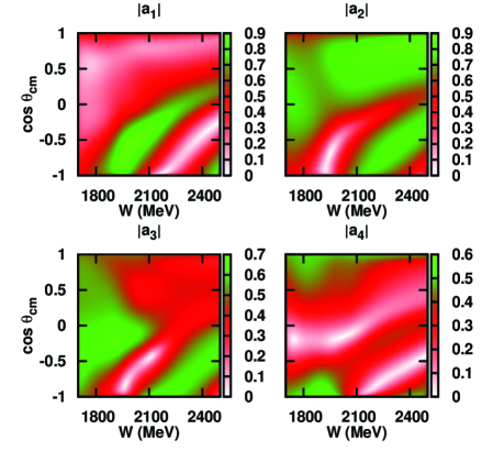
Figure 1: The RPR-2011 predictions for the energy and kaon-angle dependence of the moduli $r_{i}=|a_{i}|$ of the NTA for the $p(\gamma,K^{+})\Lambda$ reaction.

The normalized transversity amplitudes (NTA) [18] are defined in the following way:

$$a_{i}\equiv\frac{b_{i}}{\sqrt{\sum_{i=1}^{i=4}\left|b_{i}\right|^{2}}}=\frac{b_{i}}{\sqrt{\frac{4}{K}\frac{d\sigma}{d\Omega}}}\;.$$ (5)

The NTA provide complete information about the $N(\gamma,M)X$ tranversity amplitudes $\left\{b_{1},b_{2},b_{3},b_{4}\right\}$ after measuring the differential cross section. Given the four TA, one can determine the amplitudes in any quantization basis by means of a unitary transformation [18, 25]. As can be appreciated from Table 1, any polarization observable can be expressed in terms of linear and nonlinear equations of bilinear products of the $a_{i}$. For given kinematics $\left(W,\theta_{\textrm{\footnotesize{c.m.}}}\right)$, the NTA $a_{k}\equiv r_{k}\exp\left(i\alpha_{k}\right)$ are fully determined by six real numbers conveniently expressed as three real moduli $r_{k=1,2,3}$ $\;\biggl{(}r_{4}=\sqrt{1-\sum_{k=1}^{k=3}r_{k}^{2}}\biggr{)}$ and three real relative phases $\delta_{k=1,2,3}\equiv\alpha_{k=1,2,3}-\alpha_{4}$. Only three phases are relevant as all $N(\gamma,M)X$ observables are invariant under a transformation of the type $\alpha_{k=1,2,3,4}\rightarrow\alpha_{k=1,2,3,4}+\beta$, with $\beta\in\mathbb{R}$ an arbitrary overall phase. The moduli of the NTA lie on a unit three-sphere in four dimensions:

$$r_{1}^{2}+r_{2}^{2}+r_{3}^{2}+r_{4}^{2}=1\;.$$ (6)

Choosing $\alpha_{4}=0$, the NTA obey the equation of a unit six-sphere in seven dimensions [12]:

$$\left[\textrm{Re}\left(a_{4}\right)\right]^{2}+\sum_{i=1}^{i=3}\left(\left[\textrm{Re}\left(a_{i}\right)\right]^{2}+\left[\textrm{Im}\left(a_{i}\right)\right]^{2}\right)=1\;.$$ (7)

Six real numbers are required to uniquely identify a point on a six-sphere. The NTA $a_{i}$, as defined in this work, and the Chew-Goldberger-Low-Nambu (CGLN) amplitudes $F_{i}$ are related through

$$F_{i}=U_{ij}a_{j}\sqrt{\frac{d\sigma}{d\Omega}/\rho_{0}},$$ (8)

with $\rho_{0}$ the ratio of the three-momenta of the meson and photon in the c.m. frame [25] and $U$ a unitary matrix given by [18]

$$U=-\frac{i}{\sin^{2}\theta_{\textrm{\footnotesize{c.m.}}}}\left(\begin{array}[]{*{4}{c}}i\sin\theta_{\textrm{\footnotesize{c.m.}}}e^{i\theta_{\textrm{\scriptsize{c.m.}}}}&i\sin\theta_{\textrm{\footnotesize{c.m.}}}e^{-i\theta_{\textrm{\scriptsize{c.m.}}}}&0&0\\ i\sin\theta_{\textrm{\footnotesize{c.m.}}}&i\sin\theta_{\textrm{\footnotesize{c.m.}}}&0&0\\ -e^{i\theta_{\textrm{\scriptsize{c.m.}}}}&e^{-i\theta_{\textrm{\scriptsize{c.m.}}}}&e^{i\theta_{\textrm{\scriptsize{c.m.}}}}&e^{-i\theta_{\textrm{\scriptsize{c.m.}}}}\\ 1&-1&-1&-1\end{array}\right).$$ (9)

In the remainder of this work, we consider the $p(\gamma,K^{+})\Lambda$ reaction as a prototypical example of pseudoscalar-meson photoproduction from the nucleon. Despite the fact that the cross section is several orders of magnitude smaller than those of pion photoproduction, the selfanalyzing character of the $\Lambda$ hyperon is an enormous asset for gathering a sufficiently large amount of polarization observables and achieving a status of complete information.

Before turning to an amplitude analysis of experimental data, in Fig. 1 we show model predictions for the energy and angular dependence of the $p(\gamma,K^{+})\Lambda$ normalized transversity amplitudes. We use the Regge-plus-Resonance (RPR) framework in its most recent version RPR-2011 [19, 20]. The model has a Reggeized $t$-channel background and the $s$-channel resonances $S_{11}(1535)$, $S_{11}(1650)$, $F_{15}(1680)$, $P_{13}(1720)$, $P_{11}(1900)$, $D_{13}(1900)$, $P_{13}(1900)$, and $F_{15}(2000)$. The resonance content of the RPR-2011 model was determined in a Bayesian analysis of the available data. The RPR approach provides a low-parameter framework with predictive power for $K^{+}$ and $K^{0}$ photoproduction on the proton and the deuteron [21].

Interestingly, in Fig.1 it is seen that the energy and angular dependence of the moduli of the amplitudes $r_{i}=|a_{i}|$ display some interesting features. At forward kaon angles, where most the strength resides, the $r_{2}$ plays a dominant role. The strongest variations with energy are observed at backward kaon angles. No dramatic changes in the energy dependence of the $|a_{i}|$ are observed near the poles of the $s$-channel resonances. The smooth energy dependence of the moduli at forward angles reflects the fact that RPR-2011 predicts that the reaction under consideration receives very important $t$-channel background contributions. The strongest effects from the $s$-channel resonances are predicted to occur at backward angles. In the forthcoming section it will be shown that model predictions of the type shown in Fig. 1 can already be confronted with published data.

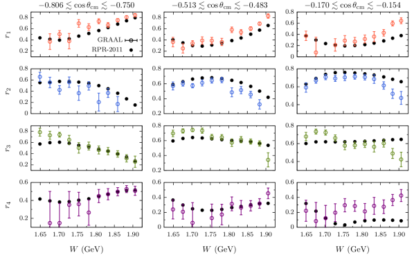
Figure 2: The moduli $r_{i}$ for $p(\gamma,K^{+})\Lambda$ as a function of $W$ at three $\cos\theta_{\textrm{\footnotesize{c.m.}}}<0$ bins. The data are extracted from the single-polarization observables of Refs. [22, 23] with the Eq. (10). The dots are the RPR-2011 predictions.

3 Results

In Table IV of Ref. [19] an overview of the published experimental data for the $p(\gamma,K^{+})\Lambda$ reaction is provided. Not surprisingly, in the quality and quantity of the experimental results, there is a natural hierarchy whereby the unpolarized data are most abundant. To date, the $p\left(\gamma,K^{+}\right)\Lambda$ data base contains 4231 measured differential cross sections, 2260 measured single-polarization observables (178 $\Sigma$, 2013 $P$, 69 $T$) and 452 data points for double-polarization observables (320 $C_{(x,z)}$ and 132 $O_{(x^{\prime},z^{\prime})}$). For an amplitude analysis, it is important to realize that the underlying physical realm is such that there are about 5 times as many $p\left(\gamma,K^{+}\right)\Lambda$ single-polarization data than double-polarization data. In view of this, the transversity representation of the amplitudes is a very promising one. Indeed, in the transversity basis the single-polarization observables are linked to the squared moduli of the NTA by means of linear equations. From Table 1 one easily finds that the squared NTA moduli can be directly obtained from

$$\left\{\begin{array}[]{ll}r_{1}^{2}=\frac{1}{4}\left(1+\Sigma+T+P\right),\\ r_{2}^{2}=\frac{1}{4}\left(1+\Sigma-T-P\right),\\ r_{3}^{2}=\frac{1}{4}\left(1-\Sigma-T+P\right),\\ r_{4}^{2}=\frac{1}{4}\left(1-\Sigma+T-P\right)\;.\end{array}\right.$$ (10)

Accordingly, a measurement of $\left(\Sigma,T,P\right)$ at given $(W,\cos\theta_{\textrm{\footnotesize{c.m.}}})$ provides good prospects to infer the moduli $r_{i}(W,\cos\theta_{\textrm{\footnotesize{c.m.}}})$ of the NTA. We now illustrate this with published data. The GRAAL collaboration [22, 23] provides $p(\gamma,K^{+})\Lambda$ data for $\left\{\Sigma,T,P\right\}$ at 66 $(W,\cos\theta_{\textrm{\footnotesize{c.m.}}})$ combinations in the ranges $1.65\lesssim W\lesssim 1.91$ GeV (with a bin width of $\Delta W\approx 50$ MeV) and $-0.81\lesssim\cos\theta_{\textrm{\footnotesize{c.m.}}}\lesssim 0.86$ (with a bin width of $\Delta\cos\theta_{\textrm{\footnotesize{c.m.}}}\approx 0.3$). Figure 2 shows a selection of the extracted $r_{i}$ at three $\theta_{\textrm{\footnotesize{c.m.}}}$ intervals in the backward kaon hemisphere along with the RPR-2011 predictions. For 7 out of a total of 131 points, the $r_{i}$ could not be retrieved from the data. This occurs whenever one or more terms of the right-hand side of Eq. (10) are negative due to finite experimental error bars. Note that there is negative correlation between the magnitude of $r_{i}$ and the size of the error bar $\Delta r_{i}$. Moreover, the smaller the $r_{i}$ the larger the probability that it cannot be retrieved from the $\left\{\Sigma,T,P\right\}$ data. From Fig. 2 it is further clear that the RPR-2011 model offers a reasonable description of the magnitude and $W$ dependence of the extracted $r_{i}$. At forward angles (not shown here) the data confirm the predicted dominance of $r_{2}$ [18]. Another striking feature of Fig. 2 is the rather soft energy and angular dependence of the moduli. As a matter of fact, the accomplished energy and angular resolution of the GRAAL data really suffices to map the moduli of the NTA in sufficient detail.

The above discussion illustrates that extraction of the moduli from measured single-polarization observables can be successfully completed in over 90% of the kinematic situations, given the present accuracy of the data. Given information about values of the NTA moduli, inferring the NTA phases $\left\{\delta_{1},\delta_{2},\delta_{3}\right\}$ from data requires measured double asymmetries. Some discrete ambiguities arise from the nonlinear character of the equations that connect the data to the underlying phases. We illustrate this with an example using the complete set $\{{\Sigma,P,T},C_{x},O_{x},E,F\}$. From the expressions of Table 1 one readily finds [17, 18]

$$\left\{\begin{array}[]{ll}{r_{1}r_{4}}\sin\delta_{1}+{r_{2}r_{3}}\sin\Delta_{23}=-\frac{C_{x}}{2},\\ {r_{1}r_{4}}\cos\delta_{1}+{r_{2}r_{3}}\cos\Delta_{23}=+\frac{O_{x}}{2},\\ {r_{1}r_{3}}\cos\Delta_{13}-{r_{2}r_{4}}\cos\delta_{2}=+\frac{E}{2},\\ {r_{1}r_{3}}\sin\Delta_{13}+{r_{2}r_{4}}\sin\delta_{2}=-\frac{F}{2}\;,\end{array}\right.$$ (11)

where two independent $\delta_{i}$ and two dependent phases $\Delta_{ij}$ have been introduced:

$$\delta_{i}\equiv\alpha_{i}-\alpha_{4}\hskip 21.68231pt\textrm{and,}\hskip 21.68231pt\Delta_{ij}=\delta_{i}-\delta_{j}\;.$$ (12)

After determining the $r_{i}$, measured $\left\{C_{x},O_{x}\right\}$ allow one to compute $\left\{\delta_{1},\Delta_{23}\right\}$, while data for $\left\{E,F\right\}$ yield $\left\{\delta_{2},\Delta_{13}\right\}$. Upon solving the above set for the cosine of a specific angle one finds two solutions. The equation for the sine is used to determine the quadrant in which each angle lies. This means that upon solving the above set of four equations, there are four possible combinations of angles $\left\{\delta_{1},\delta_{2},\Delta_{13},\Delta_{23}\right\}$ which are compatible with the double-polarization data given the moduli $\left\{r_{1},r_{2},r_{3},r_{4}\right\}$. We stress that in the transversity basis, single-polarization observables are part of any complete set as they provide the information about the NTA moduli. From the four possible solutions for the $\left\{\delta_{1},\delta_{2},\Delta_{13},\Delta_{23}\right\}$ of Eq. (11), the physical one can, in principle, be selected from the trivial condition

$$\delta_{1}-\Delta_{13}-\delta_{2}+\Delta_{23}=0\;.$$ (13)

Several types of complete sets can be distinguished. Complete sets necessarily involve double-polarization observables of two different kinds, for example the combination of $\mathcal{B}\mathcal{R}$ and $\mathcal{B}\mathcal{T}$. In this work we consider complete sets of the first kind and complete sets of the second kind. The abovementioned set $\{{\Sigma,P,T},C_{x},O_{x},E,F\}$ is a prototypical example of a complete set of the first kind with four possible solutions to the phases. A similar procedure applied to complete sets of the second kind, for example $\{{\Sigma,P,T},C_{x},O_{x},E,H\}$, leads to eight solutions.

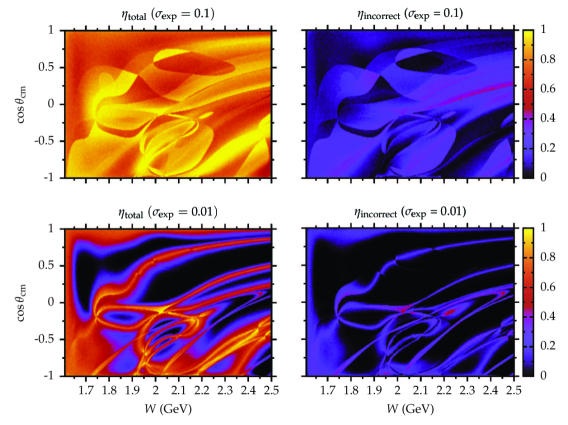
Figure 3: The energy and angular dependence of the insolvabilities $\eta_{\textrm{\footnotesize{total}}}$ ($\eta_{\textrm{\footnotesize{incorrect}}}$) at two values of the experimental accuracy. The pseudo data for the complete set $\{\Sigma,P,T,C_{x},O_{x},E,F\}$ are generated with the RPR-2011 model.

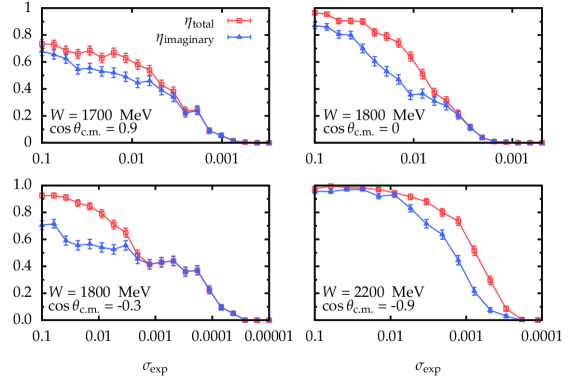
Figure 4: The insolvability of the NTA as a function of the experimental accuracy at four different kinematical points. The data are generated from the complete set $\{\Sigma,P,T,C_{x},O_{x},E,F\}$. The squares (triangles) are the $\eta_{\textrm{\footnotesize{total}}}$ ($\eta_{\textrm{\footnotesize{imaginary}}}$) insolvability.

To date, the published double-polarization observables $\{C_{x},C_{z},O_{x^{\prime}},O_{z^{\prime}}\}$ for $p\left(\gamma,K^{+}\right)\Lambda$ are of the $\mathcal{B}\mathcal{R}$ type and do not comprise a complete set, as, to our knowledge, neither $\mathcal{B}\mathcal{T}$ nor $\mathcal{T}\mathcal{R}$ data is available. In order to assess the potential to retrieve the NTA phases from double-polarization data with finite error bars, we have conducted studies with pseudo data generated by the RPR-2011 model for $p\left(\gamma,K^{+}\right)\Lambda$. We have considered ensembles of 200 pseudo data sets for $\{\Sigma,P,T,C_{x},O_{x},E,F\}$ in a fine grid of kinematic conditions. The pseudo data for all observables are drawn from Gaussians with the RPR-2011 prediction as mean and a given experimental accuracy $\sigma_{\textrm{\footnotesize{exp}}}$ determining the standard deviation. The retrieved $\{r_{i=1,2,3,4},\delta_{i=1,2,3}\}$ from analyzing the pseudo data with the aid of Eqs. (10), (11) and (13) do not necessarily comply with the RPR-2011 input amplitudes, to which we will refer as the “actual solutions”. There are various sources of error:

• imaginary solutions for the moduli upon solving the set of Eq. (10) with input values of $\{\Sigma,P,T\}$,

• imaginary solutions for the phases upon solving a set of the type of Eq. (11) with input values for four different double-polarization observables,

• incorrect solutions which stem from the fact that the condition of Eq. (13) cannot be exactly obeyed for data with finite errors. Thereby, the most likely solution does not necessarily coincide with the actual one.

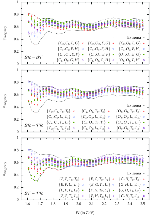
Figure 5: The energy dependence of the $\eta_{\textrm{\footnotesize{imaginary}}}$ for $\sigma_{\textrm{\footnotesize{exp}}}=0.1$. We consider all 36 complete sets of the first kind of the $\mathcal{B}\mathcal{R}$, $\mathcal{B}\mathcal{T}$, and $\mathcal{T}\mathcal{R}$ type. Also shown is the minimum and maximum value of $\eta_{\textrm{\footnotesize{imaginary}}}$.

The insolvability $\eta$ at a specific kinematic point $\left(W,\cos\theta_{\textrm{\footnotesize{c.m.}}}\right)$ is introduced as the fraction of simulated complete data sets that are solved incorrectly or have imaginary solutions:

$$\eta_{\textrm{\footnotesize{total}}}=\eta_{\textrm{\footnotesize{incorrect}}}+\eta_{\textrm{\footnotesize{imaginary}}}\;.$$ (14)

In the simulations, we first check whether all values of the retrieved NTA phases and moduli are real. Subsequently, we check whether those extracted real values for $\{r_{i=1,2,3,4},\delta_{i=1,2,3}\}$ coincide with the “actual’ ones. As an example, $\eta_{\textrm{\footnotesize{incorrect}}}=0.4$ indicates that $40\%$ of the evaluated sets of “complete” pseudo data that provide real solutions, are incorrect. For, $\eta_{\textrm{\footnotesize{total}}}=0$ the actual NTA can be retrieved in all considered sets of pseudo data. Figure 3 shows the angular and energy dependence of the insolvabilities for the complete set $\{\Sigma,P,T,C_{x},O_{x},E,F\}$. It can be concluded that for realistic experimental accuracies of the order of 10% of an asymmetry’s maximum possible value (corresponding with $\sigma_{\textrm{\footnotesize{exp}}}=0.1$) the $\eta_{\textrm{\footnotesize{total}}}$ are quite substantial and of the order 0.6–0.7. Thereby, the largest contribution is from the imaginary solutions upon determining the NTA phases from measured double asymmetries. Figure 4 illustrates that increasing the experimental resolution clearly improves the overall solvability. In the limit of vanishing error bars, the complete sets of observables do, indeed, allow one to retrieve the full information about the NTA from the data. For achievable experimental accuracies this is unfortunately not the case in the majority of situations.

Although incorrect solutions make up the smaller contribution to $\eta_{\textrm{\footnotesize{total}}}$, they can never really be identified in an analysis of real data without invoking a model. Incorrect solutions originate from assigning the most likely solution as the actual solution, which is not a statistically sound procedure. A more conservative approach would consist of imposing a tolerance level on the confidence interval of the most likely solution. Then, the most likely solution would be accepted as the actual one if it has a certain minimum statistical significance. As discussed at the end of Sec. IV C 2 in Ref. [18], however, imposing a tolerance confidence level would not be effective as the entire elimination of the incorrect solutions would lead to a rejection of the lion’s share of the fraction of correct solutions. This would result in an almost 100% insolvability.

The above conclusions about the possibility to determine the NTA from “complete” sets are based on a statistical analysis of pseudo data for $\{\Sigma,P,T,C_{x},O_{x},E,F\}$. We now address the question whether there are large differences between the various complete sets for retrieving the NTA. To this end, we have performed simulations for all 36 complete sets of the first kind. We find that $\eta_{\textrm{\footnotesize{imaginary}}}$ is consistently the most important source of NTA extraction failure. The results of our simulations are displayed in Fig. 5. It can be concluded that for $\sigma_{\textrm{\footnotesize{exp}}}=0.1$ and $W\gtrsim 1.8$ GeV, the $\eta_{\textrm{\footnotesize{imaginary}}}$ cluster around 0.6-0.7 for all 36 complete sets of the first kind. Larger variations are observed in the threshold region. This means that for the bulk of the kinematic conditions, no combination of observables performs any better than others. The results of Fig. 5 involve an averaging over $\cos\theta_{\textrm{\footnotesize{c.m.}}}$.

4 Conclusion

We have addressed the issue of extracting the reaction amplitudes from pseudoscalar-meson photoproduction experiments involving single-polarization and double-polarization observables. A possible roadmap for reaching a status of complete information in those reactions has been sketched. We suggest that the use of transversity amplitudes is tailored to the situation that experimental information about the single-polarization observables $\{\Sigma,P,T\}$ is more abundant (and most often more precise) than for the double-polarization observables. Linear equations directly connect $\{\Sigma,P,T\}$ to the squared moduli $r_{i=1,2,3,4}^{2}$ of the normalized transversity amplitudes. From an analysis of available $p(\gamma,K^{+})\Lambda$ single-polarization data, we could extract the $r_{i}$ in the majority of considered kinematic situations. Extracting the NTA independent phases is far more challenging as the equations which link them to the double asymmetries are nonlinear. Using studies with pseudo data, we have found that for currently achievable experimental accuracies, the actual phases cannot be extracted in the majority of situations. Overcomplete sets which involve more than four double asymmetries considerably improve on this figure of merit and these are subject of current investigations.

References

References

- [1] Pasyuk E and the CLAS collaboration 2012 Meson photoproduction experiments with CLAS EPJ Web Conf. 37 06013
- [2] Klein F J (CLAS Collaboration) 2012 Complete pseudoscalar photo-production experiments AIP Conf. Proc. 1432 51
- [3] D’Angelo A et al. (GRAAL Collaboration) 2012 Results from polarized experiments at LEGS and GRAAL AIP Conf. Proc. 1432 56
- [4] Arends H-J 2012 Highlights of experiments at MAMI AIP Conf. Proc. 1432 142
- [5] Klein F 2012 Highlights of experiments at ELSA AIP Conf. Proc. 1432 150
- [6] Kamano H, Nakamura S X, Lee T-S H and Sato T 2013 Nucleon resonances within a dynamical coupled-channels model of and reactions Phys. Rev. C 88 035209
- [7] Rönchen D et al. 2013 Coupled-channel dynamics in the reactions , , , Eur. Phys. J. A 49 44
- [8] Anisovich A V, Beck R, Klempt E, Nikonov V A , Sarantsev A V and Thoma U 2012 Pion- and photo-induced transition amplitudes to and Eur. Phys. J. A 48 88
- [9] The Mainz Microtron at the University of Mainz http://www.kph.uni-mainz.de/
- [10] The Elektronen-Stretcher-Anlage am Physikalischen Institut der Rheinischen Friedrich-Wilhelms-Universität Bonn http://www-elsa.physik.uni-bonn.de/
- [11] The electron accelerator at Jefferson Lab http:/www.jlab.org/
- [12] Ireland D G 2010 Information content of polarization measurements Phys. Rev. C 82 025204
- [13] Arenhövel H, Leidemann W, Tomusiak E L 1998 On complete sets of polarization observables Nucl. Phys. A 641 517
- [14] Wunderlich Y, Beck R and Tiator L 2014 The complete-experiment problem of photoproduction of pseudoscalar mesons in a truncated partial-wave analysis Phys. Rev. C 89 055203
- [15] Barker I S, Donnachie A and Storrow J K 1975 Complete experiments in pseudoscalar photoproduction Nucl. Phys. B 95 347
- [16] Keaton G and Workman R 1996 Amplitude ambiguities in pseudoscalar meson photoproduction Phys. Rev. C 53 1434
- [17] Chiang W-T and Tabakin F 1997 Completeness rules for spin observables in pseudoscalar meson photoproduction Phys. Rev. C 55 2054
- [18] Vrancx T, Ryckebusch J, Van Cuyck T and Vancraeyveld P 2013 Incompleteness of complete pseudoscalar-meson photoproduction Phys. Rev. C 87 055205
- [19] De Cruz L, Ryckebusch J, Vrancx T and Vancraeyveld P 2012 A Bayesian analysis of kaon photoproduction with the Regge-plus-resonance model Phys. Rev. C 86 015212
- [20] De Cruz L, Vrancx T, Vancraeyveld P and Ryckebusch J 2012 Bayesian inference of the resonance content of Phys. Rev. Lett. 108 182002
- [21] Vancraeyveld P, De Cruz L, Ryckebusch J and Vrancx T 2013 Kaon photoproduction from the deuteron in a Regge-plus-resonance approach Nucl. Phys. A 897 42
- [22] Lleres A et al. (GRAAL Collaboration) 2007 Polarization observable measurements for and for energies up to 1.5 GeV Eur. Phys. J. A 31 79
- [23] Lleres A et al. (GRAAL Collaboration) 2009 Measurement of beam-recoil observables , and target asymmetry for the reaction Eur. Phys. J. A 39 149
- [24] Workman R L, Paris M W, Briscoe W J, Tiator L, Schumann S, Ostrick M and Kamalov S S 2011 Model dependence of single-energy fits to pion photoproduction data Eur. Phys. J. 47 143
- [25] Sandorfi A M, Hoblit S, Kamano H and Lee T-S H 2011 Determining pseudoscalar meson photoproduction amplitudes from complete experiments J. Phys. G 38 053001