Reconstructing the final state of Pb+Pb collisions at TeV
Abstract
We fit the single-hadron transverse-momentum spectra measured in Pb+Pb collisions at TeV with the blast-wave model that includes production via resonance decays. Common fit to pions, kaons, (anti)protons, and lambdas yields centrality dependence of the freeze-out temperature and transverse expansion velocity. In the most central collisions we see MeV and . The resonance fits into this picture but the meson might freeze-out a little earlier. Multistrange baryons seem to decouple at higher temperature and weaker transverse flow. Within our model we observe hints of chemical potential for the charged pions.
pacs:
25.75.-q,25.75.Dw,25.75.Ld1 Introduction
Hot nuclear matter created in ultrarelativistic heavy-ion collisions exhibits its properties through the collective expansion of the fireball. In addition to the longitudinal flow which is largely set by the initial transparency of the nuclei, pressure gradients drive strong expansion also perpendicularly to the collision axis. Due to expansion and cooling the fireball eventually arrives to the state where it disintegrates. This is the moment when most abundant hadrons obtain their observed momenta and momentum spectra are frozen-out. In fact, it does not happen instantaneously for all hadrons. Freeze-out is a continuous process.
It is useful to describe the freeze-out state of the fireball by hydrodynamically inspired parametrisations. They usually assume that freeze-out happens instantaneously along some hypersurface. The models include locally thermalized momentum distribution and some pattern of longitudinal and transverse expansion flow velocity. A few parametrisations are on the market [1, 2, 3, 4, 5, 6] which differ in details of the assumptions for the density and velocity profiles or the exact shape of the freeze-out hypersurface. In our analysis we shall make use of the so-called blast-wave model [3].
An important part of final state hadrons does not originate directly from the fireball but comes from decays of unstable resonances which themselves were emitted from the fireball. Hadron production by resonance decays is clearly substantial for pions. However, it also contributes largely to protons and kaons, as we will show below. In spite of this, it is often omitted in calculations and analyses due to its computational complexity [7, 8, 9].
In this paper we compare Monte-Carlo-generated transverse momentum spectra with the data measured in Pb+Pb collisions at TeV by ALICE collaboration [10]. Our simulation follows the prescription of the blast-wave model. The Monte Carlo treatment has been chosen because in this way we are able to include also the resonance production of hadrons into the simulation. A similar analysis of RHIC spectra can be found in [11].
This allows us to deduce the values of kinetic freeze-out temperature and transverse expansion velocity much more reliably than in fits with only direct thermal production included, e.g. [10].
In the next Section we briefly summarize the relevant features of our Monte Carlo model—the package DRAGON [12]. In Section 3 we study how resonance production of hadrons affects spectra. As a cross-check of our approach we have also performed an analysis identical to [10] and then show how results change if resonances are included. Our main results are presented in Section 4. We have fitted spectra of pions, kaons, (anti)protons, and ’s [13] and also looked at ’s and ’s [14]. From the resulting fireball freeze-out parameters we calculated spectra of and and compared them with the measured data [15]. We show our values of the parameters for six different centrality classes. Multistrange baryons seem to drop out of the systematics that describes other hadrons. Conclusions are drawn in Section 5.
2 The model
Our analysis is performed in framework of the blast-wave model, which is characterised by its emission function. Formally, it is the Wigner phase-space density of the source of hadrons of type
| (1) | |||||
Because of the dominant expansion in the longitudinal direction one uses longitudinal proper time and space-time rapidity . Polar coordinates , are used in the transverse plane. We use proper quantum statistical distributions with for fermions (bosons) and is the spin degeneracy. Every isospin state is treated separately. This prescription assumes sharp freeze-out along the hypersurface and uniform density distribution within the radius . This means that our freeze-out time does not depend on radial coordinate111This is one of the differences between our model and the Cracow single freeze-out model [16] which was used in fits to spectra measured by ALICE collaboration recently [17, 18, 19]. . The expansion of the fireball is represented by the velocity field
| (2) |
where the transverse velocity is such that
| (3) |
In this relation parametrises transverse flow gradient and the profile of the transverse velocity. The mean transverse velocity is then
| (4) |
The transverse size and the freeze-out proper time influence total normalizations of transverse momentum spectra. However, in this study we ignore those and hence we have no sensitivity to these geometric parameters.
From the emission function, spectrum of directly produced hadrons is obtained as
| (5) |
where the integration runs over the whole freeze-out hypersurface. If one replaces the quantum-statistical distribution in eq. (1) by the classical Boltzmann distribution and performs some of the integrations in eq. (5), one arrives at
| (6) |
This formula is rather easy to evaluate and thus it is often used in spectra fitting.
Resonances are emitted as described by the emission function in eq. (1) and then decay exponentially in time according to their width. All matrix elements for the decays are assumed to be constant and thus the decay is determined by the phase-space only. In principle, one can derive the emission function that includes hadrons from resonance decays [3] but the expression—unlike eq. (6)—is not suitable for massively multiple use in the fitting procedure.
Therefore, we generate stable hadrons and also resonances according to distribution and the assumption of chemical equilibrium. Resonances are then let to decay so that in the end we look only at stable hadrons. In our simulation we will systematically vary the temperature , transverse flow gradient , and the power . We construct histograms in for some number of Monte Carlo events for each set of parameters which are then compared with measured data and a value of is obtained. This procedure is rather CPU and storage-demanding because the generation must be done separately for each set of parameters that we want to check.
The share of hadrons coming from resonance decays in our model is set at the chemical freeze-out specified by MeV and [20]. Note that shifting these values slightly is not expected to cause a big change in the shape of the transverse momentum spectra.
This value of chemical freeze-out temperature was found to reproduce the ratios of hadron multiplicities [20] and we keep it in order to satisfy that observation. Since the thermal freeze-out temperature is lower, we actually assume here that the time between chemical and thermal freeze-out is so short that the majority of resonances does not decay so that their products would rescatter. The opposite extreme scenario (not studied here) is that strong interactions regenerate some number of resonances. This must happen so that the state of partial chemical equilibrium is established, because the final observed numbers of stable hadrons is fixed to the values that correspond to the chemical freeze-out state. Thus in partial chemical equilibrium the loss of pions due to fewer resonances that decay would have to be exactly compensated by the increase of the number of direct pions. The real scenario may likely be somewhere in between these two extreme models. Another possibility is the scenario with single chemical and thermal freeze-out [17, 18]. As mentioned above, due to fast transverse expansion at the LHC, here we assume only short time between chemical and thermal freeze-out which keeps basically all resonances according to the chemical freeze-out temperature. At the chemical freeze-out, all hadrons are produced from the same common volume. Then, in the short time of further expansion the volume occupied by each species may be slightly different due to the difference in their thermal velocities. Same kind of model has been applied also in an analysis of nuclear collisions at RHIC energies [11].
3 Impact of resonance decays on transverse momentum spectra
Data from Pb+Pb collisions at TeV were measured by the ALICE collaboration. Spectra of the most abundant species—pions, kaons, protons and antiprotons—were published in [10] along with a simple thermal fit to the spectra which included only directly produced particles and no resonance decay effect. An effort has been made to identify fiducial intervals in where the influence of resonance decays can be omitted. They were for pions, for kaons and for protons. As we first wanted to set the benchmark and compare our method to other analyses, we performed the same blast-wave model fit with the same fiducial intervals as [10] using our Monte Carlo approach instead of eq. (6).
Event samples were generated for different sets of parameters . The parameter space was sampled so that the step in temperature was 4 MeV, the step in was 0.01, and the step in was 0.02 or 0.04. Each of these steps induces roughly the same amount of change in the resulting spectra. The step size was compromised in view of the CPU time required and has impact on the precision with which we can locate the parameter set that fits the data best. Explored parameter sets were chosen so that we always explore large enough region in parameter space around the best fit.
We checked that the generated spectra are accurately described by eq. (6) with appropriate parameters. Then we looked for the parameter set for which Monte Carlo data show the best match with measured data using the minimum method. Results are summarised in Table 1. They agree with those by ALICE collaboration [10] reasonably well.
-
ALICE [10] no resonances with resonances centrality (MeV) (MeV) (MeV) 0–5% 95 0.651 0.71 98 0.645 0.73 82 0.662 0.69 5–10% 97 0.646 0.72 98 0.645 0.73 94 0.654 0.69 10–20% 99 0.639 0.74 102 0.637 0.73 90 0.649 0.71 20–30% 101 0.625 0.78 102 0.624 0.79 98 0.633 0.75 30–40% 106 0.604 0.84 110 0.605 0.81 102 0.616 0.79 40–50% 112 0.574 0.94 110 0.572 0.97 118 0.581 0.89 50–60% 118 0.535 1.10 122 0.527 1.15 126 0.541 1.03 60–70% 129 0.489 1.29 126 0.484 1.39 146 0.489 1.23 70–80% 139 0.438 1.58 142 0.439 1.51 170 0.423 1.55
Then, in order to check whether resonances can indeed be neglected in the fiducial range, we added resonance decays to our Monte Carlo data. Their contribution is characterised by the chemical freeze-out temperature as described in the previous section. We still kept the limitation to the fiducial intervals. Results are summarised in Table 1. The extracted kinetic freeze-out temperatures changed and the direction in which they have gone depends on centrality. For central collisions the temperature was lowered while for peripheral ones it went up. It thus seems that leaving out resonances is not a good approximation even if one tries to identify a reasonable fiducial range for the fitting.
To support this statement we have analysed our Monte Carlo events and looked at the number of hadrons emitted directly and the number coming from the decays of resonances.
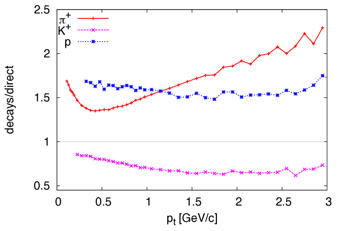
In Fig. 1 we plot the ratio of hadrons produced from the resonance decays to those produced directly as functions of . They are calculated for model parameters which best fit the spectra in most central collisions (see Table 2). The portion of resonance production is very important not only for pions but also for kaons and protons. Moreover, the ratio shows nontrivial dependence. One might omit resonances in the fitting procedure in a region where these ratios are constant but there is no such interval for any of the investigated species. For pions the -dependence is even non-monotonic. Hence, leaving out resonances is an invalid simplification.
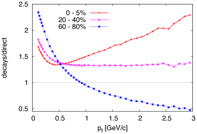
We analysed the resonance contribution to hadron spectra in much detail. In Fig. 2 we demonstrate that the relative contribution of resonance decays to pion production also depends on kinetic freeze-out temperature and transverse flow. Simulated data correspond to best fits in the indicated centrality classes (next Section). The rise of decays/direct ratio with increasing is due to decays of resonances with masses so high that pions get large kinetic energy from their decays. In central collisions the freeze-out temperature is low. Thus at higher the pion spectrum is dominated by heavy resonance decay products. It also helps that these resonances are boosted due to large transverse velocity of the part of fireball which emits them. In peripheral collisions the freeze-out temperature increases and the transverse flow is weaker. The former gives high to direct pions and the latter gives less boost to heavy resonances. As a result, the contribution of resonance production decreases with growing .
4 Fits to hadron transverse momentum spectra
In our actual analysis we fitted spectra of pions, charged kaons, protons and antiprotons [10] together with spectra of ’s and ’s [13]. Our simulations were further compared with spectra of multistrange baryons and published in [14]. Finally, we compared with data [15] our predictions for and which were based on the results of fits to , , , , and .
The and hyperon data are divided into fewer centrality classes than data from , , , and . In order to make consistent fits which include all species, we used the centrality classes of hyperon spectra and summed up corresponding centrality bins in pion, kaon, and proton spectra. Error bars of experimental data points were taken as statistical and systematic added in quadrature.
The parameter space was sampled as described in the previous section. After having all ensembles of events simulated we compared them with data. Histograms of simulated data were normalized individually so that their normalization matches that of experimental spectrum. Among all simulated ensembles we found the one which best agrees with the data (the minimum ). We chose this procedure in order to find the best fits to the shape of the spectrum which is sensitive to the dynamical state of the fireball at the freeze-out. Their normalization, on the other hand, requires the volume which is best reconstructed in common analysis with femtoscopy data.
Fit results depend on the cuts imposed on the spectra. For each species we specified a high- cut. This is justified, because from some value of upwards hadrons are expected to be more influenced by hard production processes and not described by the thermal model we use. To find the cuts we determined ratios of measured-to-simulated bin content for each species as a function of . Then, those bins from the high- end of the spectra for which the value of was outside the range (0.9, 1.1) were excluded, effectively introducing high- cuts. (The chosen range was found to lead to best fits.) In the next step, Monte Carlo data were again compared with the data without excluded bins. This time, new high- cuts were determined and the procedure was repeated again. The iterations were stopped when they converged to one set of parameters and certain set of cuts.
For pions, we imposed also a low cut at 400 MeV/, thus not including the first 9 bins into the comparison. We found that the quality of the fit significantly deteriorated without this cut. It seems that pion spectra show an enhancement here which might be due to non-equilibrium pion chemical potential not included in our simulation.
Here we did not try to come up with a fit function using Tsallis distribution that would cover the whole interval [21, 22, 23]. Its interpretation in terms of thermal model would be unclear.
4.1 Spectra of
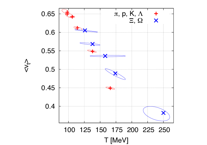
We first fitted spectra for the most abundant species: pions, kaons, (anti)protons, ’s, and ’s. In Fig. 3 we show positions of the best fits for each centrality.
Note that in the actual fitting procedure we determined three parameters: , , and . In order to compare results in a relevant way we have plotted here the positions of the best fits in just two parameters, and , with the latter calculated from eq. (4) for the values of that give the minimum of . As can also be seen in Table 2, with the change of centrality, sometimes changes due to a change in and not in .
-
centrality (MeV) 0–5% 98 0.88 0.69 0.654 0.214 194 5–10% 98 0.88 0.71 0.649 0.266 197 10–20% 106 0.87 0.71 0.642 0.272 210 20–40% 114 0.86 0.81 0.612 0.294 202 40–60% 138 0.82 0.99 0.548 0.347 195 60–80% 166 0.77 1.43 0.449 0.449 168
In Table 2 the fitted values are displayed together with their and the number of degrees of freedom. In Fig. 3 they are displayed together with our estimates for the uncertainty region for the best fit values. We stress that these are only estimates because the evaluation of in discrete points does not allow us to determine them more precisely. We observe that the position of minimum determines very precisely the value of . For the temperature, the uncertainty is larger. It may range up to 10–15 MeV from the minimum.
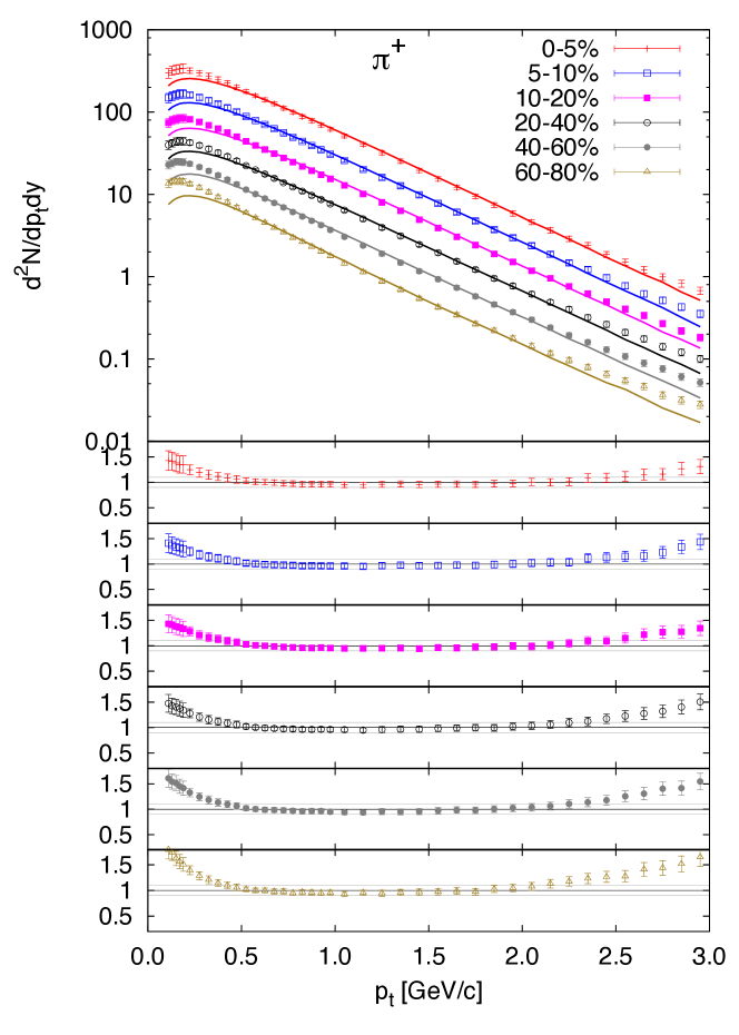
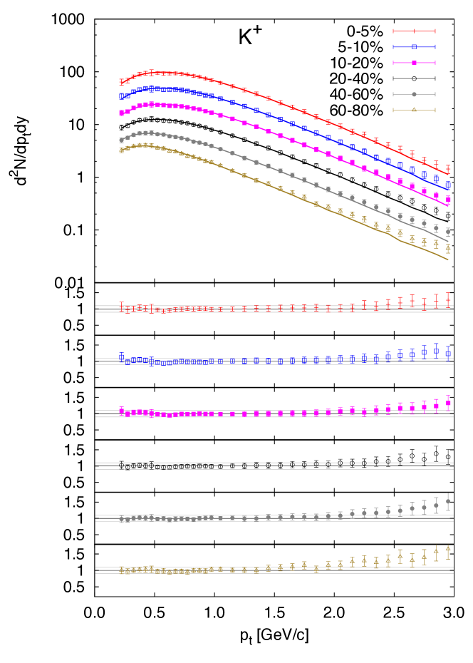
We illustrate the quality of the fits in Figs. 4–8. For brevity, for the most abundant spectra we only show the comparison with positively charged species and note that the comparison looks the same for negative species. For pions (Fig. 4) we clearly see the enhancement at low . Recall that our fitting procedure does not include any chemical potential but we account for resonance production. For pions at below 400 MeV/, resonance contribution grows as is lowered. This can be observed in Fig. 1. Still, although qualitatively this behaviour might agree with what is seen in data, quantitatively it is not sufficient to explain them. Resonances tend to populate low- region but this is not enough to fit the data. We speculate that the solution might be in introducing non-equilibrium chemical potential for pions. This would naturally occur if the hadron gas chemically freezes out at a temperature around 150–160 MeV and then cools down while keeping the effective ratios of individual species constant. We estimated that the pion chemical potential at kinetic freeze-out temperature might reach values around 100 MeV. This is not enough for Bose-Einstein condensation but modifies the spectrum considerably.
In the higher- region the pion spectrum is well reproduced up to about 2 GeV. This seems reasonable, as for higher we may see signs of hard production.
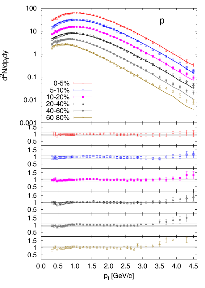
Charged kaons (Fig. 5) are well reproduced in a similar interval without the need to leave out any bins at low . We also observe good fits to (anti)proton spectrum (Fig. 6) stretching out even to about 4 GeV. In general, the agreement becomes slightly worse when going away from central collisions. For the most peripheral class charged kaons depart from the theoretical curve above 2 GeV/ and protons above 3.5 GeV/.
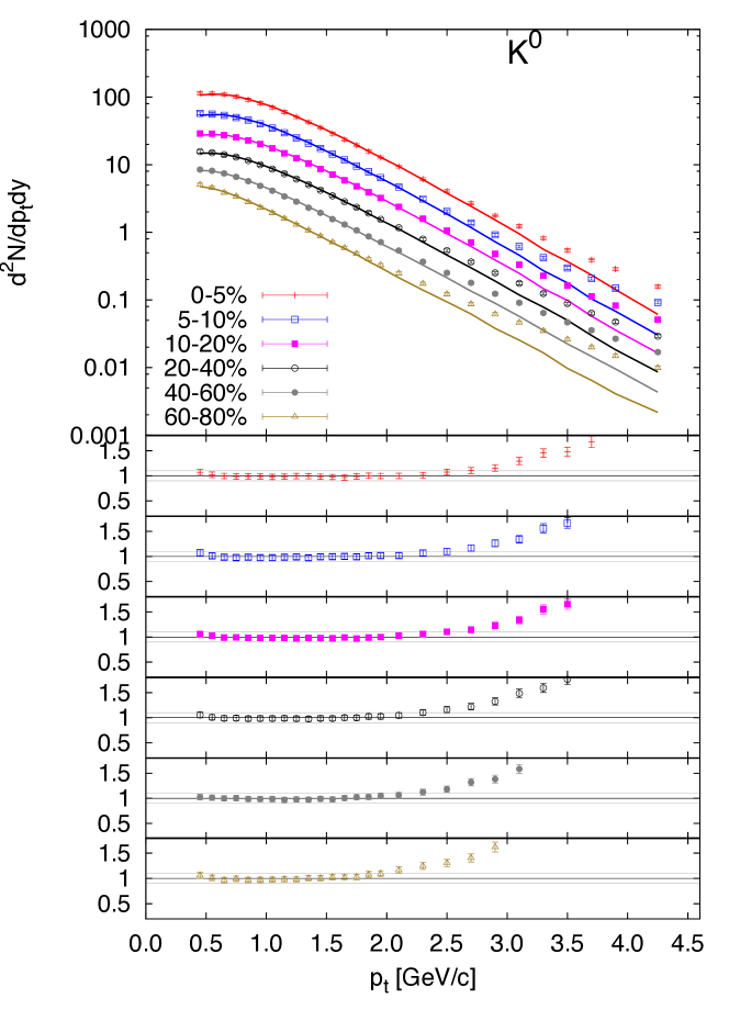
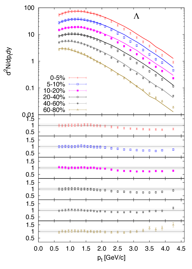
In the fit we also included strange ’s which were measured up to of 4.5 GeV/ [13]. The kaons show (Fig. 7) similar behaviour as their charged isospin partners. When comparing the two plots for (Fig. 5) and (Fig. 7) one should notice the different intervals in which these spectra are measured. Below the cut of 2 GeV also the ’s are fitted well (Fig. 8). They slightly depart from this agreement above 2 GeV, but in a different way than other species: ’s are steeper at high than the thermal fits. Note that the values of freeze-out parameters were determined in common fits to all 8 species, including ’s. We might be seeing here the beginning of the departure of strange baryon spectra from the scenario of common freeze-out. Note, however, that the departure occurs for above 2 GeV/ where thermal hydrodynamically inspired model should not be given too much stress.
4.2 Spectra of , , , and
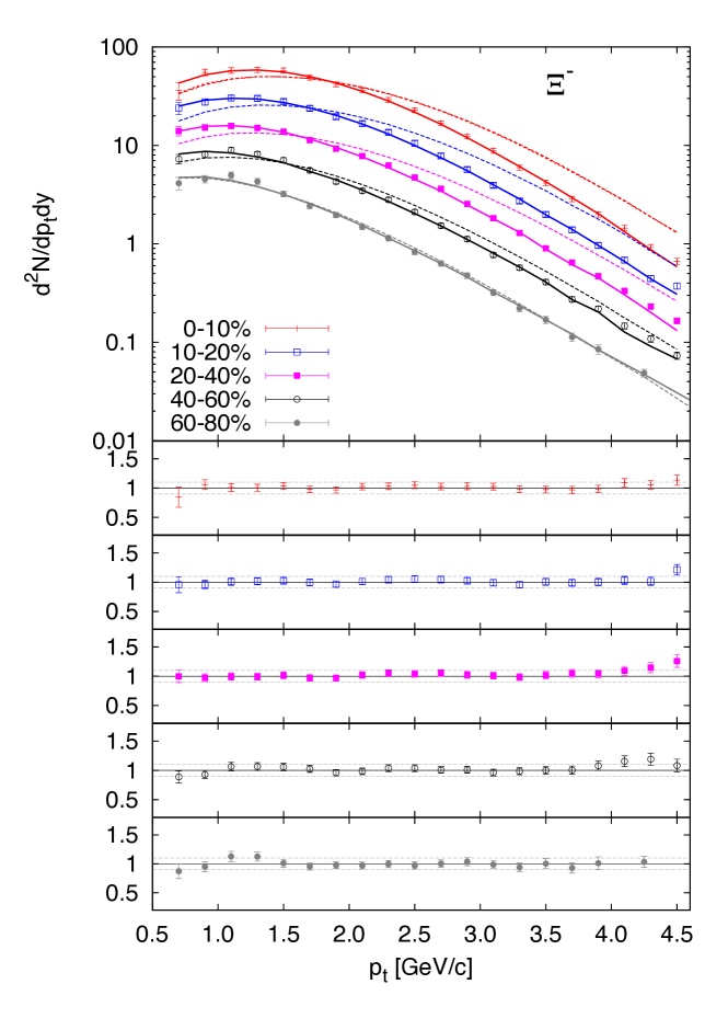
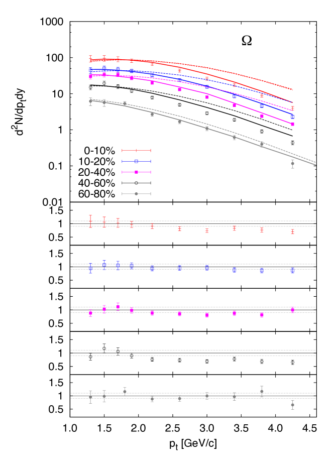
The departure of data from the model fitted in previous subsection is clearly seen when we focus on spectra of multiply strange baryons: , , , and . We show only the spectra of baryons in Fig. 9 () and Fig. 10 (). Results for antibaryons are similar. Note that these species were not included in the previous fitting procedure. In order to check whether they fit into the same description of the fireball we have simulated their spectra in DRAGON with the sets of parameters that come from the fits to , , , , (Table 2). These predictions are plotted in Figs. 9 and 10 by dashed curves. We notice that in general the data are steeper than the prediction. The data would thus indicate lower transverse expansion velocities and earlier freeze-out of multiply strange baryons [24]. Note, however, that for the two most peripheral classes the agreement of data and prediction becomes better.
In order to quantify this statement we have performed common fits to the four multistrange baryon species: , , , and and extracted their values of , , and corresponding . They are listed in Table 3 and compared with the other fit results in Fig. 3.
-
centrality (MeV) 0–10% 126 0.82 0.71 0.605 0.375 41 10–20% 138 0.81 0.85 0.568 0.325 41 20–40% 158 0.78 0.91 0.536 0.417 37 40–60% 174 0.76 1.11 0.489 0.497 33 60–80% 250 0.64 1.35 0.382 0.795 39
This clearly shows the general effect that multiply strange baryons seem to decouple at higher temperature and weaker transverse expansion. The fitted spectra are compared to data in Figs. 9 and 10 by solid lines. Due to higher statistics, fit results seem to be driven by the ’s rather than by ’s. Although it is hard to support it statistically, it seems that the spectrum is even steeper than the fit results. This would indicate even lower expansion velocity at the moment of decoupling.
Looking at the most peripheral centrality class we notice that the measured data seem to be well reproduced by both sets of fit results. Note that the freeze-out temperature in peripheral collisions is higher than in the central ones. The spectra in those collisions are thus less sensitive to the mass of particles. What we see here is an illustration of the ambiguity in determination of and . Lower temperature can be compensated by stronger flow and vice-versa. When spectra depend on the mass, this ambiguity is usually resolved by different shapes of spectra of different species. Figure 3 indicates that statistically one can still resolve the fit to multistrange baryons as the uniquely correct result.
4.3 Spectra of and
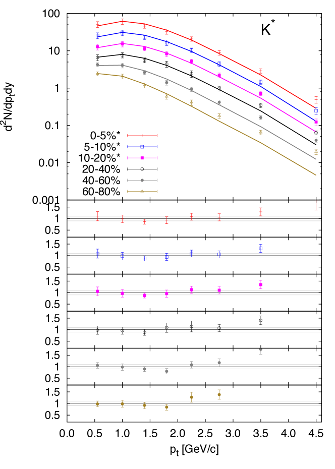
ALICE collaboration has also published transverse momentum spectra of resonances and [15]. Studying resonances may reveal information about the dynamics of the fireball, particularly its evolution between chemical and thermal freeze-out. In order to simulate these resonances we have forbidden them to decay in our Monte Carlo generator since by default their decay is turned on. We simulated their spectra with the parameters from Table 2 and compare them with data in Figs. 11 and 12. Hence, they have not been fitted in our treatment. We observe reasonably good agreement of theory with data in centrality classes 0–20% and 20–40% and below 2 GeV/ for the . For higher the data tend to be flatter than the theory.
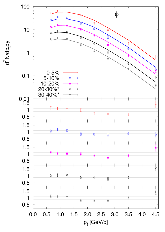
The meson with its mass 1.02 GeV/ is an important probe of fireball dynamics. If it is produced from the thermalized fireball at the common freeze-out, then its spectrum must be close to that of protons. In Fig. 12 we compare the data with predictions based on parameters from Table 2. Data seem to be slightly steeper than the prediction. This is best seen in the ratios plotted in the lower panels of the Figure. Such a disagreement might indicate slightly earlier freeze-out from the fireball. Note, however, that the deviation of the prediction from the data is much smaller than in the case of multistrange baryons and no indisputable sign of earlier decoupling can be claimed.
5 Conclusions
The blast-wave model with hadron production from resonance decays included can well reproduce single-particle spectra measured by ALICE collaboration in Pb+Pb collisions at TeV. Resonance contribution leads to shifts in the values of freeze-out parameters. For central collisions our freeze-out temperatures tend to be lower than those extracted by ALICE [10]. On the other hand, the temperatures shift in the opposite direction for peripheral collisions. Shifts in have smaller relative size.
Multistrange baryons show freeze-out at higher temperature and weaker transverse flow. This is consistent with earlier decoupling from the fireball. Note that such a behaviour is known from SPS [24] and RHIC [25] data, as well.
In fits to data from most peripheral collisions we obtain temperatures for kinetic freeze-out that are higher than what is usually assumed for the chemical freeze-out. On one side we can take this result as a parametrisation and the values of parameters are those which fit the data best. However, as soon as we want to interpret these values in the framework of some scenario for the fireball evolution, we may be witnessing limitations of the used model.
In principle, our assumption of chemical equilibrium may seem inconsistent with individual normalisation of each spectrum as we performed it. If different spectra are multiplied with different factors this can be seen as effectively changing relative numbers of final state species. Caution would be particularly in place if we tried to predict the absolute yields of final hadron species. Here, however, we wanted to enhance the sensitivity to and and thus we focussed on the shapes of the spectra which remain intact by the individual normalizations. Indeed, although rescaling one spectrum might have an influence on another one through changing yields of resonances which also contribute to a different final state species (like e.g. contributing to pions and nucleons), this does not tie different spectra too strongly together. The reason is that the main contributing resonance decays are different for different hadron species: for pions the most important are , , [26]; for protons the resonance; for the and hyperons; for kaons the . Thus rescaling the yield for one species does not have much influence on another species.
A more complete analysis would include also the model interpretation of the normalisations which are given by the volume. Such an analysis, however, must include femtoscopy and is planned for the future.
Similar fits were performed recently with the Cracow single freeze-out model [17, 18]. The main feature of that model is common chemical and thermal freeze-out with non-equilibrium fugacities introduced for strange and also non-strange species. Due to this, the freeze-out temperature fitted there is generally higher than our results. Note however, that their freeze-out hypersurface has a different shape. Naturally, this opens the question if one can distinguish between the two models. Perhaps femtoscopy can provide the tool for this task.
It is an intriguing speculation if the two approaches may be equivalent. Here we recall the scenario that matter hadronizes and cools down while keeping partial chemical equilibrium. This leads to the appearance of non-equilibrium chemical potentials for all species, i.e. chemical potentials that are not given by chemical potentials of conserved quantum numbers [27]. In the single freeze-out model, on the other hand, the system is born into the chemical non-equilibrium. We wonder how close to this non-equilibrium state the fireball comes in the cooling fireball scenario.
A comprehensive picture of the gradual fireball cooling should also include earlier decoupling of multistrange baryons.
Finally, let us come back to the issue that our results have been obtained in a scenario which assumes different chemical and thermal freeze-out and the difference between their temperatures is rather high. If one would revisit the question of the evolution between them, the inclusion of chemical potentials may be important. They may have influence on the shape of spectra especially for pions and we seem to observe the corresponding features in the data. This task will be addressed in a subsequent paper.
References
- [1] P. J. Siemens and J. O. Rasmussen, Phys. Rev. Lett. 42, 880 (1979).
- [2] K. S. Lee and U. Heinz, Z. Phys. C 43, 425 (1989).
- [3] E. Schnedermann, J. Sollfrank and U. Heinz, Phys. Rev. C 48, 2462 (1993) [nucl-th/9307020].
- [4] T. Csörgő and B. Lörstad, Phys. Rev. C 54, 1390 (1996) [hep-ph/9509213].
- [5] B. Tomášik, U. A. Wiedemann and U. Heinz, Heavy Ion Phys. 17, 105 (2003) [nucl-th/9907096].
- [6] F. Retiere and M. A. Lisa, Phys. Rev. C 70, 044907 (2004) [nucl-th/0312024].
- [7] J. Sollfrank, P. Koch and U. Heinz, Phys. Lett. B 252, 256 (1990).
- [8] J. Sollfrank, P. Koch and U. Heinz, Z. Phys. C 52, 593 (1991).
- [9] U. A. Wiedemann and U. Heinz, Phys. Rev. C 56, 3265 (1997) [nucl-th/9611031].
- [10] B. Abelev et al. [ALICE collaboration], Phys. Rev. C 88, 044910 (2013).
- [11] S Choi and K S Lee, Phys. Rev. C 84 (2011) 064905
- [12] B. Tomášik, Comput. Phys. Commun. 180, 1642 (2009) [arXiv:0806.4770 [nucl-th]].
- [13] B. Abelev et al. [ALICE collaboration], Phys. Rev. Lett. 111, 222301 (2014).
- [14] B. Abelev et al. [ALICE collaboration], Phys. Lett. B 728, 216 (2014).
- [15] B. Abelev et al. [ALICE Collaboration], arXiv:1404.0495 [nucl-ex].
- [16] W. Broniowski and W. Florkowski, Phys. Rev. Lett. 87, 272302 (2001) [nucl-th/0106050].
- [17] V. Begun, W. Florkowski and M. Rybczyński, Phys. Rev. C 90, no. 1, 014906 (2014) [arXiv:1312.1487 [nucl-th]].
- [18] V. Begun, W. Florkowski and M. Rybczyński, Phys. Rev. C 90, no. 5, 054912 (2014) [arXiv:1405.7252 [hep-ph]].
- [19] S. Chatterjee, B. Mohanty and R. Singh, Phys. Rev. C 92 (2015) 2, 024917 [arXiv:1411.1718 [nucl-th]].
- [20] L. Milano [ALICE Collaboration], Nucl. Phys. A 904-905, 531c (2013) [arXiv:1302.6624 [hep-ex]].
- [21] G. Wilk and Z. Wlodarczyk, Eur. Phys. J. A 40, 299 (2009) [arXiv:0810.2939 [hep-ph]].
- [22] J. Cleymans, G. Hamar, P. Lévai and S. Wheaton, J. Phys. G 36, 064018 (2009) [arXiv:0812.1471 [hep-ph]].
- [23] H. R. Wei, F. H. Liu and R. A. Lacey, arXiv:1509.09083 [nucl-ex].
- [24] H. van Hecke, H. Sorge and N. Xu, Phys. Rev. Lett. 81, 5764 (1998) [nucl-th/9804035].
- [25] J. Adams et al. [STAR Collaboration], Phys. Rev. Lett. 92, 182301 (2004) [nucl-ex/0307024].
- [26] I. Melo, B. Tomášik, arXiv:1509.05383 [nucl-th].
- [27] H. Bebie, P. Gerber, J. L. Goity and H. Leutwyler, Nucl. Phys. B 378, 95 (1992).
