$\boldsymbol{Wb\bar{b}j}$ production at NLO with POWHEG+MiNLO

Abstract:

We present a next-to-leading order plus parton-shower event generator for the production of a $W$ boson plus two bottom quarks and a jet at hadron colliders, implemented in the POWHEG BOX framework. Bottom-mass effects and spin correlations of the decay products of the $W$ boson are fully taken into account. The code has been automatically generated using the two available interfaces to MadGraph4 and GoSam, the last one updated to a new version. We have applied the MiNLO prescription to our $Wb\bar{b}j$ calculation, obtaining a finite differential cross section also in the limit of vanishing jet transverse momentum. Furthermore, we have compared several key distributions for $Wb\bar{b}j$ production with those generated with a next-to-leading order plus parton-shower event generator for $Wb\bar{b}$ production, and studied their factorization- and renormalization-scale dependence. Finally, we have compared our results with recent experimental data from the ATLAS and CMS Collaborations.

1 Introduction

The production of a $W$ boson in association with two $b$ jets at hadron collider has many interesting experimental and theoretical facets. On the experimental side, more interest for this process has been recently driven by the discovery of a light scalar particle [1, 2], whose characteristics point to make it a suitable candidate for being the Higgs boson responsible for the spontaneous symmetry breaking of the Standard Model. In this respect, $Wb\bar{b}+X$ is an irreducible background for $HW$ production, with the Higgs boson decaying into $b$ quarks. In addition, it is also a background to single top and top-pair production, where the top quark decays into a $Wb$ pair, and to many new physics searches.

On the theoretical side, the calculation of differential cross sections at hadronic colliders in the presence of massive quarks is surely more challenging than with massless partons. In addition, the presence of logarithmic-enhanced terms of ratios of the quark mass over higher scales may invalidate the perturbative expansion in the strong coupling constant $\alpha_{\mathchoice{\displaystyle}{\scriptstyle}{\scriptscriptstyle}{\scriptscriptstyle}\rm S}$ (see also ref. [3] for a recent review of the subject).

$Wb\bar{b}$ production at next-to-leading order (NLO) in QCD has been studied for a while [4, 5, 6, 7, 8]. All these calculations were performed in the so-called 4-flavour scheme, where the $b$ quark is treated as massive (except for ref. [4], where the bottom quark is massless) and there is no direct contribution from the $b$ parton-distribution function in the incoming hadrons. $Wb+X$ production in the 5-flavour scheme, where the $b$ quark is treated as massless and there is a contribution from the $b$ parton-distribution function, is discussed, for example, in refs. [9, 10, 11]. $Wb\bar{b}$ production is also available in NLO+parton-shower (NLO+PS) event generators such as the POWHEG BOX [12] and MC@NLO [8].

In this paper we present a NLO calculation for $Wb\bar{b}$ + 1 jet production interfaced with the POWHEG method [13, 14] and distributed as part of the POWHEG BOX package [15]. Bottom-mass effects and spin correlations of the leptonic decay products of the $W$ boson have been fully taken into account. In the following we will refer to this event generator as Wbbj.

The Born, real, spin- and colour-correlated Born amplitudes have been generated automatically using the interface of MadGraph4 [16, 17] to the POWHEG BOX [18]. The virtual contribution has also been computed automatically using the interface [19] to GoSam [20, 21].

With the straightforward use of these two interfaces we have also generated a new code for $Wb\bar{b}$ production at NLO, with exact spin correlations in the decay of the $W$ boson into leptons. We will refer to this event generator as Wbb. In ref. [12], $Wb\bar{b}$ production was interfaced with the POWHEG method, and the $W$ decay was simulated in an approximated way. We made several comparisons between the generator described in ref. [12] and the new Wbb one, studying angular and transverse-momentum distributions of the $W$ decay products, and found no sizable differences.

The choice of factorization and renormalization scale(s) for $Wb\bar{b}+X$ production is a debated issue in the scientific literature: in fact, it is well known that NLO corrections to $Wb\bar{b}$ production are quite large [6], due to the opening of gluon-initiated channels at NLO. A separate paper will be needed to discuss scale dependence more thoroughly. In this paper, we apply the MiNLO [22] procedure to our calculation, and we leave POWHEG and MiNLO to choose two of the scales at which the strong coupling constant is evaluated. This process, in fact, starts at order $\alpha_{\mathchoice{\displaystyle}{\scriptstyle}{\scriptscriptstyle}{\scriptscriptstyle}\rm S}^{3}\,\alpha_{\mathchoice{\displaystyle}{\scriptstyle}{\scriptscriptstyle}{\scriptscriptstyle}EM}^{2}$ and gets contributions up to order $\alpha_{\mathchoice{\displaystyle}{\scriptstyle}{\scriptscriptstyle}{\scriptscriptstyle}\rm S}^{4}\,\alpha_{\mathchoice{\displaystyle}{\scriptstyle}{\scriptscriptstyle}{\scriptscriptstyle}EM}^{2}$ at next-to-leading order. The advantage of using MiNLO is twofold:

1. First of all, we are left only with the choice of the scale(s) for the primary process, i.e. the underlying flavour and kinematic configuration after the clusterization operated by the MiNLO procedure.

2. We can provide event samples that are NLO+PS accurate for $Wb\bar{b}j$ production (this is by construction) but that display, at the same time, a finite differential cross section in the limit of the accompanying jet $j$ becoming soft or collinear, overlapping in this way to the Wbb results.

The paper is organized as follows: in sec. 2 we recall all the ingredients that are necessary in order to build the NLO+PS code in the POWHEG BOX, and some technical detail on the change of the renormalization scheme. In sec. 3, we illustrate the modifications to the original MiNLO procedure for the case at hand, and the scale choice(s) for the primary process. In sec. 4 we study some key distributions at the NLO and Les Houches event level, and we compare the Wbb generator with the Wbbj+MiNLO one. We present a comparison with CMS and ATLAS data in sec. 5 and we give our conclusions in sec. 6.

2 Born, real and virtual contributions

The code for the computation of the amplitudes for $Wb\bar{b}$ and $Wb\bar{b}j$ production was generated using the existing interfaces of the POWHEG BOX to MadGraph4 and GoSam [20] presented in refs. [18, 19]. The one-loop amplitudes are generated with the new version 2.0 of GoSam [21], that uses QGRAF [23], FORM [24] and SPINNEY [25] for the generation of the Feynman diagrams. They are then computed at running time with Ninja [26, 27], which is a reduction program based on the Laurent expansion of the integrand [28], and using OneLOop [29] for the evaluation of the scalar one-loop integrals. For unstable phase-space points, the reduction automatically switches to Golem95 [30], that allows to compute the same one-loop amplitude evaluating tensor integrals. Alternatively, the traditional integrand-reduction method [31], extended to $D$-dimensions [32], as implemented in SAMURAI [33], can be used.

We point out that a numeric calculation for $Wb\bar{b}j$ was performed in ref. [34] too, with the $W$ boson treated as stable, and in ref. [26], with full spin correlations in the decay of the $W$ boson. In addition, there are other automated codes that can generate the virtual contributions (see, for example, ref. [35]).

In order to run the code, the user has only to select the sign of the $W$ boson, i.e. $W^{+}$ or $W^{-}$, and its leptonic decay mode, i.e. electronic, muonic or tauonic decay, in the POWHEG BOX input file. Other flags to control the POWHEG BOX behavior are documented in previous implementations and in the Docs directory.

2.1 The decoupling and $\overline{\rm MS}$ schemes

When performing a fixed-order calculation with massive quarks, one can define two consistent renormalization schemes that describe the same physics: the usual $\overline{\rm MS}$ scheme, where all flavours are treated on equal footing, and a mixed scheme [36], that we call decoupling scheme, in which the $n_{\rm lf}$ light flavours are subtracted in the $\overline{\rm MS}$ scheme, while the heavy-flavour loop is subtracted at zero momentum. In this scheme, the heavy flavour decouples at low energies.

The virtual contributions generated by GoSam are computed in the decoupling scheme. This means that, since we are dealing with bottom-quark production, we have the correct virtual contributions if the strong coupling constant $\alpha_{\mathchoice{\displaystyle}{\scriptstyle}{\scriptscriptstyle}{\scriptscriptstyle}\rm S}$ is running with 4 light flavours, and if the appropriate parton distribution functions (pdfs) do not include the bottom quark in the evolution.

To make contact with other results expressed in terms of the ${\overline{\rm MS}}$ strong coupling constant, running with 5 light flavours, and with pdfs with 5 flavours, we prefer to change our renormalization scheme and to switch to the ${\overline{\rm MS}}$ one.

The procedure for such a switch is well known, and was discussed in ref. [37] (see Appendix A for a quick review of this procedure). For $Wb\bar{b}j$ production, we need to add to the NLO cross section, computed in the decoupling scheme, the following two terms:

• to the $qq$ initial-state channel

  $$-2\,T_{\mathchoice{\displaystyle}{\scriptstyle}{\scriptscriptstyle}{\scriptscriptstyle}\rm F}\,\frac{\alpha_{\mathchoice{\displaystyle}{\scriptstyle}{\scriptscriptstyle}{\scriptscriptstyle}\rm S}}{2\pi}\,\log\left(\frac{\mu_{\mathchoice{\displaystyle}{\scriptstyle}{\scriptscriptstyle}{\scriptscriptstyle}\rm R}^{2}}{m_{\scriptscriptstyle\rm b}^{2}}\right)\,{\cal B}_{qq}$$ (1)

• to the $qg$ initial-state channel

  $$2\,T_{\mathchoice{\displaystyle}{\scriptstyle}{\scriptscriptstyle}{\scriptscriptstyle}\rm F}\,\frac{\alpha_{\mathchoice{\displaystyle}{\scriptstyle}{\scriptscriptstyle}{\scriptscriptstyle}\rm S}}{2\pi}\left[\frac{1}{3}\log\left(\frac{\mu_{\mathchoice{\displaystyle}{\scriptstyle}{\scriptscriptstyle}{\scriptscriptstyle}\rm F}^{2}}{m_{\scriptscriptstyle\rm b}^{2}}\right)-\log\left(\frac{\mu_{\mathchoice{\displaystyle}{\scriptstyle}{\scriptscriptstyle}{\scriptscriptstyle}\rm R}^{2}}{m_{\scriptscriptstyle\rm b}^{2}}\right)\right]{\cal B}_{qg}$$ (2)

where ${\cal B}_{qq}$ and ${\cal B}_{qg}$ are the squared Born amplitude for the corresponding initial states, $\mu_{\mathchoice{\displaystyle}{\scriptstyle}{\scriptscriptstyle}{\scriptscriptstyle}\rm R}$ and $\mu_{\mathchoice{\displaystyle}{\scriptstyle}{\scriptscriptstyle}{\scriptscriptstyle}\rm F}$ are the renormalization and factorization scale, respectively, and $m_{\scriptscriptstyle\rm b}$ is the bottom-quark mass.

2.2 LO and NLO comparisons

In this section we perform a comparison between the leading order (LO) and next-to-leading order results for $Wb\bar{b}j$ production, using a static renormalization and factorization scale.

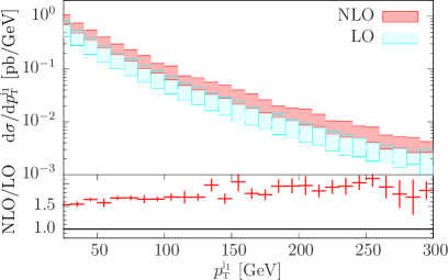
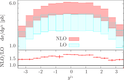
Figure 1: Transverse momentum (left) and rapidity distribution (right) of the hardest jet in $Wb\bar{b}j$ production. NLO and LO scale-variation bands are obtained as explained in the text. In the lower insert, we plot the ratio of the NLO over the LO result, computed with the central scale. The corresponding integration statistical error is also shown.

We present results for $W^{+}$ production at the LHC at 14 TeV. Similar results can be obtained for $W^{-}$ production. We have set the renormalization and factorization scale equal to $\mu$

$$\mu_{\mathchoice{\displaystyle}{\scriptstyle}{\scriptscriptstyle}{\scriptscriptstyle}\rm R}=\mu_{\mathchoice{\displaystyle}{\scriptstyle}{\scriptscriptstyle}{\scriptscriptstyle}\rm F}=\mu$$ (3)

and varied $\mu$ in the range $\mu=\{m_{\mathchoice{\displaystyle}{\scriptstyle}{\scriptscriptstyle}{\scriptscriptstyle}W}/2,m_{\mathchoice{\displaystyle}{\scriptstyle}{\scriptscriptstyle}{\scriptscriptstyle}W},2\,m_{\mathchoice{\displaystyle}{\scriptstyle}{\scriptscriptstyle}{\scriptscriptstyle}W}\}$. Jets and other physical parameters are defined as in sec. 4 and a minimum cut on the hardest jet of 25 GeV has been imposed, in order to have finite distributions. The total cross sections for the central scale are

$$\sigma_{\mathchoice{\displaystyle}{\scriptstyle}{\scriptscriptstyle}{\scriptscriptstyle}\rm LO}=17.3~{}{\rm pb},\qquad\qquad\sigma_{\mathchoice{\displaystyle}{\scriptstyle}{\scriptscriptstyle}{\scriptscriptstyle}\rm NLO}=28.4~{}{\rm pb}.$$ (4)

By varying the renormalization and factorization scale we have a 46% variation for the LO total cross and a 29% variation at NLO, showing a significative reduction of the scale dependence. In fig. 1 we compare two differential distributions, i.e. the transverse momentum and rapidity of the hardest jet, at leading and next-to-leading order. A reduction on the scale dependence is clear in the two panels.

In the rest of the paper we abandon the use of a fixed scale, since we leave to MiNLO [22] the choice of scales. Being interested in a shower Monte Carlo simulation, the most appropriate scale for the evaluation of the strong coupling constant associated with the emission of a jet is the transverse momentum of the jet itself, provided the suitable Sudakov form factor is attached, as done by the MiNLO procedure. We will further illustrate our use of the MiNLO procedure in the next section.

3 MiNLO

The MiNLO procedure [22] has already been applied successfully to several production processes: $H/Z/Wj$ [38], $W/Zjj$ [39], $HVj$ [19], trijet [40], $W\gamma$ [41] production. In $H/Z/Wj$ and $HVj$ production, a slightly modified version of the original MiNLO formalism [38] allowed to reach NLO accuracy for inclusive quantities with one less jet too, i.e. $H/W/Z$ and $HV$ production, respectively. With the same modified version and with the additional knowledge of the fixed NNLO differential cross section [42, 43], Higgs boson [44, 45] and Drell-Yan [46] production could be simulated at NNLO+PS accuracy.

Unfortunately, for $Wb\bar{b}j$ production, no such modification of the MiNLO Sudakov form factor is known (due to the presence of coloured particles in the final state that complicates the structure of the resummation formulae), and we cannot demonstrate that we can generate an event sample with NLO accuracy for $Wb\bar{b}$ production too. We will limit ourselves to show that we can generate a $Wb\bar{b}j$ event sample with finite differential cross section down to the transverse momentum of the hardest jet $j$ going to zero, and to show that it agrees fairly well with the cross section obtained with the Wbb event generator for $Wb\bar{b}$ production.

Our last remark concerns the clusterization procedure operated by MiNLO: since no collinear singularities are associated with the final-state $b$ quarks, the clusterization procedure is not applied to the heavy quarks. In this way, if the event gets clustered, then we have to deal with the kinematics of a $Wb\bar{b}$ configuration, otherwise we have a $Wb\bar{b}j$ one.

3.1 Wbb and Wbbj+MiNLO scale choice

$Wb\bar{b}$ and $Wb\bar{b}j$ production are multi-scale processes. The investigation of the dependence of the differential cross section on different scale choices is fundamental to assess the uncertainties on the theoretical predictions and in the comparison with the experimental data. In sec. 4, we limit ourselves to present results at a given dynamical scale and we compute scale-variation bands around it. In sec. 5, we present a few results at a different scale when we compare our theoretical predictions with the ATLAS data.

Our default scale choice is the following:

1. In the Wbb generator, we have set the renormalization and factorization scales equal to

   $$\mu_{\mathchoice{\displaystyle}{\scriptstyle}{\scriptscriptstyle}{\scriptscriptstyle}\rm R}=\mu_{\mathchoice{\displaystyle}{\scriptstyle}{\scriptscriptstyle}{\scriptscriptstyle}\rm F}=\mu\equiv\frac{E_{B}}{4}\,,{\rm\quad where\quad}E_{B}=\sqrt{\hat{s}}\,,{\rm\quad and\quad}\hat{s}=(p_{\mathchoice{\displaystyle}{\scriptstyle}{\scriptscriptstyle}{\scriptscriptstyle}\rm W}+p_{\mathchoice{\displaystyle}{\scriptstyle}{\scriptscriptstyle}{\scriptscriptstyle}\rm b}+p_{\mathchoice{\displaystyle}{\scriptstyle}{\scriptscriptstyle}{\scriptscriptstyle}\rm\bar{b}})^{2},$$ (5)

   where $p_{\mathchoice{\displaystyle}{\scriptstyle}{\scriptscriptstyle}{\scriptscriptstyle}\rm W}$, $p_{\mathchoice{\displaystyle}{\scriptstyle}{\scriptscriptstyle}{\scriptscriptstyle}\rm b}$ and $p_{\mathchoice{\displaystyle}{\scriptstyle}{\scriptscriptstyle}{\scriptscriptstyle}\rm\bar{b}}$ are the momenta of the $W$ boson, of the $b$ and $\bar{b}$ quark respectively, at the underlying-Born level, i.e. the kinematic configuration on top of which the POWHEG BOX attaches the hard radiated parton with the appropriate Sudakov form factor.

2. In the Wbbj+MiNLO generator, we have the freedom to set the scale(s) of the primary process. We have fixed this scale to be the same scale $E_{B}$ of eq. (5), where now $p_{\mathchoice{\displaystyle}{\scriptstyle}{\scriptscriptstyle}{\scriptscriptstyle}\rm W}$, $p_{\mathchoice{\displaystyle}{\scriptstyle}{\scriptscriptstyle}{\scriptscriptstyle}\rm b}$ and $p_{\mathchoice{\displaystyle}{\scriptstyle}{\scriptscriptstyle}{\scriptscriptstyle}\rm\bar{b}}$ are the momenta of the $W$, $b$ and $\bar{b}$ in the primary process if there has been a clusterization. If the event has not been clustered by the MiNLO procedure, i.e. if the underlying Born $Wb\bar{b}j$ process is not clustered by MiNLO, we take as scale the partonic center-of-mass energy of the event.

With these scale choices, we have good agreement between the the Wbb and Wbbj+MiNLO results, as will be shown in sec. 4.2. The fact that the scale in the Wbb generator is smaller than the scale of the primary process in the Wbbj+MiNLO generator is a common feature of the MiNLO procedure. In fact, it has already been observed in vector-boson and Higgs boson production plus jet [22, 39, 19], and in trijet production [40].

4 Results

In this section, we present our findings for the LHC at 7 TeV. We have set the $b$ quark mass at the value $m_{b}=4.75$ GeV and we have used the MSTW2008 [47] pdf. Clearly, any other pdf could have been used.

The CKM matrix has been set to

$$\begin{array}[]{c}\\ V_{\rm\mathchoice{\displaystyle}{\scriptstyle}{\scriptscriptstyle}{\scriptscriptstyle}CKM}=\end{array}\begin{array}[]{c c}&d\quad\quad\ \ s\ \ \quad\quad b\\ \begin{array}[]{c}u\\ c\\ t\end{array}&\left(\begin{array}[]{c c c}0.97428&0.2253&0.00347\\ 0.2252&0.97345&0.041\\ 0.00862&0.0403&0.999152\end{array}\right).\end{array}$$ (6)

Since the experimental data for $Wb\bar{b}$ production are presented as summed over $W^{+}$ and $W^{-}$ production, we do the same in our plots.

Jets are reconstructed using the anti-$k_{\mathchoice{\displaystyle}{\scriptstyle}{\scriptscriptstyle}{\scriptscriptstyle}\rm T}$ algorithm [48] as implemented in the Fastjet package [49, 50], with jet radius $R=0.7$. A minimum transverse-momentum cut of 1 GeV has been imposed to all the jets. No cuts on $b$-jets have been imposed. In all our results, the MiNLO procedure has always been turned on and events have been showered and hadronized by PYTHIA (version 6.4.25) [51], with the AMBT1 tune (call to PYTUNE(340)).

4.1 NLO and Les Houches event comparisons

In this section, we compare a few interesting kinematic distributions at the NLO level and at the Les Houches event (LHE) level, i.e. after the first hard emission generated with the POWHEG method.

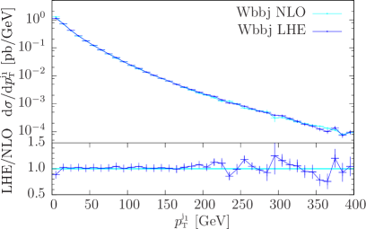
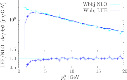
Figure 2: Transverse-momentum distribution of the hardest jet at NLO and LHE level.

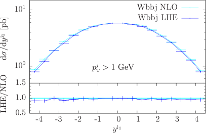
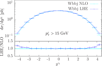
Figure 3: Rapidity distribution of the hardest jet at NLO and LHE level.

We first compare the transverse momentum and rapidity of the first hardest jet, that are predicted by the Wbbj generator with next-to-leading order accuracy.

In fig. 2, we plot the transverse momentum of the hardest jet $p_{\mathchoice{\displaystyle}{\scriptstyle}{\scriptscriptstyle}{\scriptscriptstyle}\rm T}^{\mathchoice{\displaystyle}{\scriptstyle}{\scriptscriptstyle}{\scriptscriptstyle}\rm j_{1}}$ at NLO and LHE level. The agreement is very good over a wide kinematic range. In the right panel, the low $p_{\mathchoice{\displaystyle}{\scriptstyle}{\scriptscriptstyle}{\scriptscriptstyle}\rm T}^{\mathchoice{\displaystyle}{\scriptstyle}{\scriptscriptstyle}{\scriptscriptstyle}\rm j_{1}}$ region is illustrated: here, the LHE distribution is finite and goes to zero due to the Sudakov form factor coming from MiNLO, applied to the primary process, and to the suppression factor associated to the produced radiation, i.e. the second jet, coming from the POWHEG Sudakov form factor. In the NLO result, the latter Sudakov form factor is absent, and the result increases.

We find very good agreement also for the rapidity of the hardest jet, $y^{\mathchoice{\displaystyle}{\scriptstyle}{\scriptscriptstyle}{\scriptscriptstyle}\rm j_{1}}$, shown in fig. 3. In the right panel, a minimum $p_{\mathchoice{\displaystyle}{\scriptstyle}{\scriptscriptstyle}{\scriptscriptstyle}\rm T}$ cut of 15 GeV on jets has been imposed.

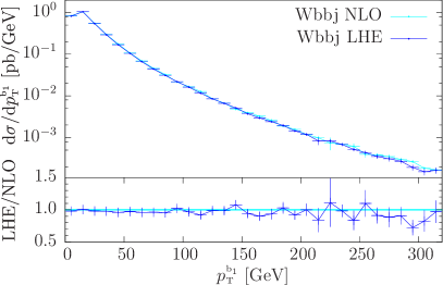
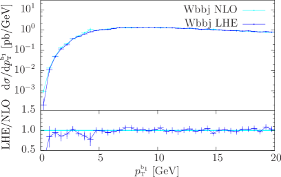
Figure 4: Transverse-momentum distribution of the hardest $b$ jet.

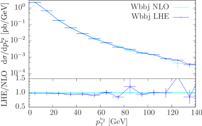
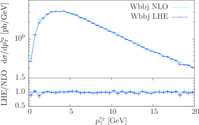
Figure 5: Transverse-momentum distribution of the next-to-hardest $b$ jet.

In figs. 4 and 5 we show the transverse-momentum distribution for the hardest and next-to-hardest $b$ jets. In both cases, the agreement between the NLO and LHE result is at the level of a few percent, over the entire $p_{\mathchoice{\displaystyle}{\scriptstyle}{\scriptscriptstyle}{\scriptscriptstyle}\rm T}$ range.

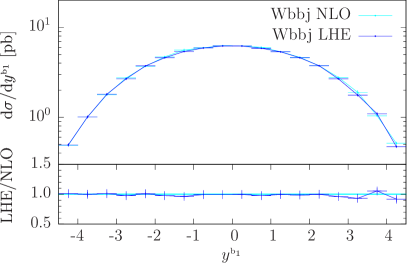
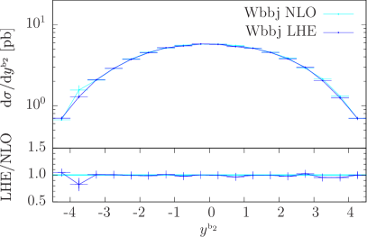
Figure 6: Rapidity distribution of the hardest (left panel) and next-to-hardest $b$ jet (right panel).

Similar conclusions hold for their rapidities, $y^{\mathchoice{\displaystyle}{\scriptstyle}{\scriptscriptstyle}{\scriptscriptstyle}\rm b_{1}}$ and $y^{\mathchoice{\displaystyle}{\scriptstyle}{\scriptscriptstyle}{\scriptscriptstyle}\rm b_{2}}$, illustrated in fig. 6.

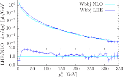
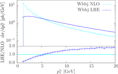
Figure 7: Transverse-momentum distribution of the next-to-hardest jet.

The transverse-momentum distribution of the next-to-hardest jet shown in fig. 7 is predicted at leading-order only. The divergent behavior at small transverse momentum in the NLO result is clearly visible in the right panel, where, instead, the POWHEG Sudakov form factor damps the LHE result.

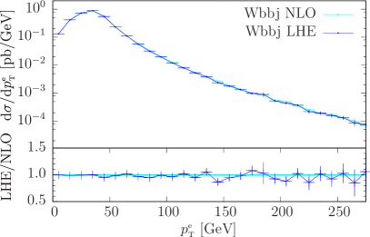
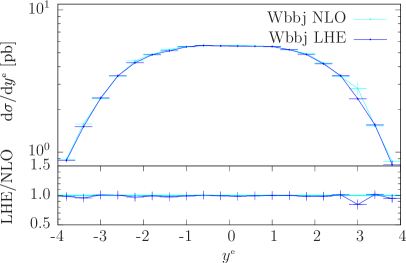
Figure 8: Transverse-momentum (left panel) and rapidity distribution (right panel) of the charged lepton from $W$-boson decay.

As last example, we plot the transverse-momentum and rapidity distribution of the charged lepton from $W$-boson decay in fig. 8, finding again very good agreement between the NLO and LHE level results.

We have compared several other kinematic distributions with different cuts and we have always found, when expected, excellent agreement between the NLO and the LHE results.

4.2 Wbb and Wbbj+MiNLO comparisons

In this section we compare key distributions for $Wb\bar{b}$ and $Wb\bar{b}j$ production, computed using the Wbb and Wbbj+MiNLO generators, respectively, in order to investigate the level of agreement between them, when the hardest jet $j$ becomes soft or collinear.

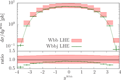
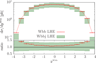
Figure 9: Rapidity distribution of the $Wb\bar{b}$ system computed with the Wbb and Wbbj+MiNLO generators, at the LHE level. In the left panel, we show the scale variation of the Wbb generator in red, and the central value of the Wbbj generator in green. In the right panel, we plot the scale variation of the Wbbj+MiNLO code in green, and the central value of the Wbb code in red. In the lower insert, we display the ratio between the maximum and the minimum of the band over the respective central value.

The rapidity $y^{\scriptscriptstyle\rm Wbb}$ of the $Wb\bar{b}$ system computed by the Wbb generator has NLO accuracy. In fact, this distribution receives contributions both at the Born level and from the virtual and real diagrams. In fig. 9 we plot such quantity, together with the same distribution as predicted by Wbbj+MiNLO.

The bands in the plots of this section are the envelope of the distributions obtained by varying the renormalization and factorization scales by a factor of 2 around the reference scale $\mu$ of eq. (5), i.e. by multiplying the factorization and the renormalization scale by the scale factors $K_{\scriptscriptstyle\rm F}$ and $K_{\scriptscriptstyle\rm R}$, respectively, where

$$(K_{\scriptscriptstyle\rm R},K_{\scriptscriptstyle\rm F})=(0.5,0.5),(0.5,1),(1,0.5),(1,1),(2,1),(1,2),(2,2).$$ (7)

These variations have been computed using the POWHEG BOX reweighting procedure, that recomputes the weight associated with an event in a fast way.

In the left panel of fig. 9, we show the scale variation of the Wbb generator in red, and the central value of the Wbbj generator in green, at the LHE level. In the right panel, we plot the scale variation of the Wbbj+MiNLO code in green, and the central value of the Wbb code in red. In the lower insert, we display the ratio between the maximum and the minimum of the band over the respective central value.

The agreement between the predictions of the Wbb and Wbbj+MiNLO generators is within the scale-variation bands. We remind the reader that, if we had used the POWHEG BOX result for $Wb\bar{b}j$ production without MiNLO, we could have not compare these distributions, since the rapidity of the $Wb\bar{b}$ system would have been divergent in the limit of the accompanying jet becoming soft or collinear with the incoming beams.

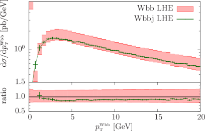
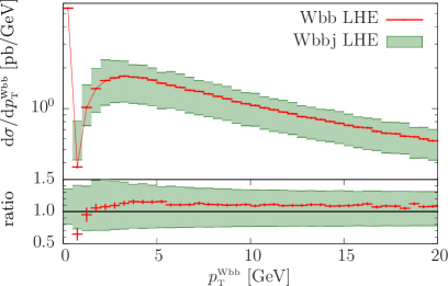
Figure 10: Same as fig. 9 but for the transverse momentum of the $Wb\bar{b}$ system.

To better illustrate the behavior of the differential cross section in the small transverse-momentum region, we compare the $p_{\mathchoice{\displaystyle}{\scriptstyle}{\scriptscriptstyle}{\scriptscriptstyle}\rm T}$ of the $Wb\bar{b}$ system obtained with the two generators in fig. 10. In $Wb\bar{b}$ production, this distribution is predicted with leading-order accuracy and the POWHEG Sudakov form factor attached to the radiation makes it finite in the small-$p_{\mathchoice{\displaystyle}{\scriptstyle}{\scriptscriptstyle}{\scriptscriptstyle}\rm T}$ region (the $Wb\bar{b}$ system recoils against the only hard jet generated by the POWHEG BOX). In $Wb\bar{b}j$ production, this distribution is finite due to the presence of the POWHEG Sudakov form factor attached to the radiation, most likely the next-to-hardest jet, and to the MiNLO Sudakov form factor, attached to the hardest jet accompanying the $Wb\bar{b}$ system. Again the agreement is very good. The finite contribution to the differential cross section visible in the first $p_{\rm\scriptscriptstyle T}^{\rm\scriptscriptstyle Wbb}$ bin, in $Wb\bar{b}$ production, is due to events that have not radiated at the LHE level.

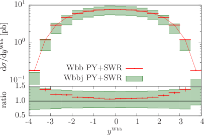
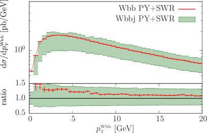
Figure 11: Rapidity and transverse momentum distribution of the $Wb\bar{b}$ system, generated by the Wbbj+MiNLO code, and showered by PYTHIA.

This peak is diluted away when the whole shower is completed by a Monte Carlo program such as PYTHIA or HERWIG [52, 53], as shown in fig. 11, right panel. In this figure, we plot the differential cross sections as a function of $y^{\scriptscriptstyle\rm Wbb}$ and $p_{\rm\scriptscriptstyle T}^{\rm\scriptscriptstyle Wbb}$ after the shower has been completed by PYTHIA. No hadronization has been switched on at this level, but we have explicitly checked that it has a negligible effect on these distributions.

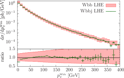
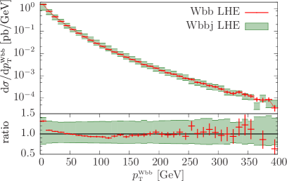
Figure 12: Same as fig. 9 but for the transverse momentum of the $Wb\bar{b}$ system.

Away from the small transverse-momentum region, the differential cross section as a function of $p_{\rm\scriptscriptstyle T}^{\rm\scriptscriptstyle Wbb}$ is predicted at LO by the Wbb generator, and at NLO by the Wbbj one. This is clearly displayed in fig. 12, where the scale variation bands for $Wb\bar{b}$ production reaches the 70%, while they are around 40% for $Wb\bar{b}j$ production.

5 Comparison with ATLAS and CMS data

In this section we compare the results that we obtained with the Wbb and Wbbj generators with the available experimental data.

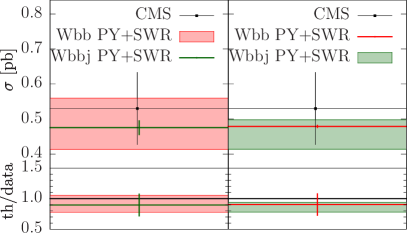
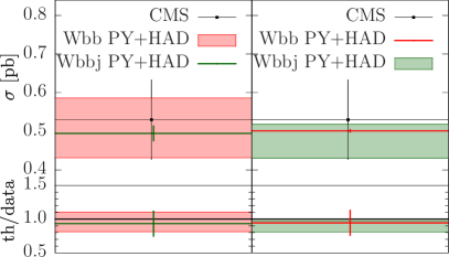
Figure 13: Total cross section for $Wb\bar{b}$ production within the cuts of eq. (9). In the left panel, the results after the shower done by PYTHIA. In the right plot, the full showered and hadronized results are shown. The measured value is compared with the results from the Wbb and Wbbj+MiNLO generators.

The CMS Collaboration has measured the $Wb\bar{b}$ cross section at the LHC at 7 TeV and the result, reported in ref. [54], is

$$\sigma(pp\to Wb\bar{b})\times{\rm BR}(W\to\mu\nu)=0.53\pm 0.10~{}{\rm pb}\,,$$ (8)

within the following experimental cuts on jets and charged leptons

$$p_{\mathchoice{\displaystyle}{\scriptstyle}{\scriptscriptstyle}{\scriptscriptstyle}\rm T}^{\mathchoice{\displaystyle}{\scriptstyle}{\scriptscriptstyle}{\scriptscriptstyle}\rm j}>25~{}{\rm GeV}\,,\quad\left|y^{\rm\mathchoice{\displaystyle}{\scriptstyle}{\scriptscriptstyle}{\scriptscriptstyle}j}\right|<2.4\,,\quad p_{\mathchoice{\displaystyle}{\scriptstyle}{\scriptscriptstyle}{\scriptscriptstyle}\rm T}^{\rm\mathchoice{\displaystyle}{\scriptstyle}{\scriptscriptstyle}{\scriptscriptstyle}e}>25~{}{\rm GeV}\,,\quad\left|y^{\rm\mathchoice{\displaystyle}{\scriptstyle}{\scriptscriptstyle}{\scriptscriptstyle}e}\right|<2.1\,,\quad\Delta R_{\rm\mathchoice{\displaystyle}{\scriptstyle}{\scriptscriptstyle}{\scriptscriptstyle}j,e}>0.5\,.$$ (9)

To reconstruct jets the anti-$k_{\mathchoice{\displaystyle}{\scriptstyle}{\scriptscriptstyle}{\scriptscriptstyle}\rm T}$ algorithm with $R=0.5$ was used and only events with exactly two jets which passed the $b$-tagging requirements were taken into account. In fig. 13 we compare our predictions with the measured value. In the left panel, we show our result after the shower done by PYTHIA, and in the right panel, the same result at the hadronic level. In particular, with the Wbb generator we have

$$\sigma(pp\to Wb\bar{b})\times{\rm BR}(W\to\ell\nu_{\ell})=0.50\,^{+0.09}_{-0.07}~{}{\rm pb}$$ (10)

and with the Wbbj+MiNLO one

$$\sigma(pp\to Wb\bar{b})\times{\rm BR}(W\to\ell\nu_{\ell})=0.49\,^{+0.03}_{-0.06}~{}{\rm pb}$$ (11)

at the hadronic level. We find very good agreement between the cross section computed with the Wbb generator and the Wbbj+MiNLO one, and both are consistent with the measured data.

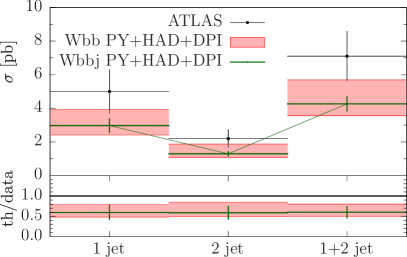
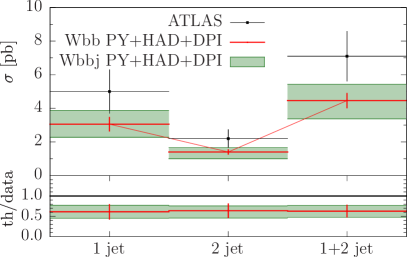
Figure 14: Cross sections, within the cuts described in the text, for the ATLAS measurement of “1 jet”, “2 jet” and “1+2 jet” $Wb$ production. The theoretical central results and error bands have been corrected for the DPI effects of tab. 1. Results are at the full shower+hadron level.

The ATLAS Collaboration reported a measurement of $W$+ $b$-jets ($W+b+X$ and $W+b\bar{b}+X$) cross section at 7 TeV in ref. [55]. Candidate $W+b$-jets events are required to have exactly one high-$p_{\mathchoice{\displaystyle}{\scriptstyle}{\scriptscriptstyle}{\scriptscriptstyle}\rm T}$ electron or muon, as well as missing transverse momentum consistent with a neutrino from a $W$ boson, and one or two reconstructed jets, exactly one of which must be $b$-tagged. Events with two or more $b$-tagged jets are rejected, as are events with three or more jets. The details of the analysis are as follows: jets are reconstructed using the anti-$k_{\mathchoice{\displaystyle}{\scriptstyle}{\scriptscriptstyle}{\scriptscriptstyle}\rm T}$ algorithm, with a radius parameter $R=0.4$, and are required to have a transverse momentum greater than 25 GeV and absolute rapidity $|y^{\mathchoice{\displaystyle}{\scriptstyle}{\scriptscriptstyle}{\scriptscriptstyle}j}|<2.1$. Furthermore the following cuts are applied

$$p_{\mathchoice{\displaystyle}{\scriptstyle}{\scriptscriptstyle}{\scriptscriptstyle}\rm T}^{\mathchoice{\displaystyle}{\scriptstyle}{\scriptscriptstyle}{\scriptscriptstyle}\rm e}>25~{}{\rm GeV}\,,\quad p_{\mathchoice{\displaystyle}{\scriptstyle}{\scriptscriptstyle}{\scriptscriptstyle}\rm T}^{\mathchoice{\displaystyle}{\scriptstyle}{\scriptscriptstyle}{\scriptscriptstyle}\rm\nu}>25~{}{\rm GeV}\,,\quad\left|y^{\mathchoice{\displaystyle}{\scriptstyle}{\scriptscriptstyle}{\scriptscriptstyle}\rm e}\right|<2.5\,,\quad m_{\mathchoice{\displaystyle}{\scriptstyle}{\scriptscriptstyle}{\scriptscriptstyle}\rm T}^{\mathchoice{\displaystyle}{\scriptstyle}{\scriptscriptstyle}{\scriptscriptstyle}\rm W^{\pm}}>60~{}{\rm GeV}\,,\quad\Delta R_{\rm\mathchoice{\displaystyle}{\scriptstyle}{\scriptscriptstyle}{\scriptscriptstyle}j,e}>0.5\,.$$ (12)

In fig. 14 we plot the ATLAS results for the measured cross-sections for the “1 jet”, “2 jet” and “1+2 jet” fiducial regions, together with our results. In the “1 jet” bin, we show the cross section with only one jet, that necessarily must contain at least one $b$ quark, or a $\bar{b}$, or both (clustered in a single jet). In the “2 jet” bin, we plot the cross section for events with two jets, only one of which is $b$-tagged. In the “1+2 jet” bin, there is the sum of the previous two cross sections.

With the same scale choice of sec. 3.1, our predictions for the “1+2 jet” bin are

$$\sigma_{\tt Wbbj}({\rm\mbox{1+2~{}jet}}) = 2.93\,^{+0.73}_{-0.59}~{}{\rm pb}$$

$$\sigma_{\tt Wbb}({\rm\mbox{1+2~{}jet}}) = 3.12\,^{+0.81}_{-0.58}~{}{\rm pb}$$ (13)

at the hadron level.

correction	1 jet	2 jet	1+2 jet
—DPI [pb]	$\ \ 1.02\,^{+0.40}_{-0.29}$	$\ \ 0.32\,^{+0.12}_{-0.09}\ \$	$1.34\,^{+0.42}_{-0.30}\ \$

Table 1: Additive corrections for double-parton interactions (DPI) as estimated by the ATLAS Collaboration. See tab. 7 in ref. [55].

Since neither the Wbb nor the Wbbj+MiNLO results contain the effect of double-parton interactions (DPI) within the same proton, we need to correct our cross sections for this. The computation of this contribution is beyond the aim of the present paper. On the other hand, the ATLAS Collaboration has estimated such effect and has provided some additive values to correct for it. We collect them in tab. 1 and after correcting for DPI, we get

$$\sigma_{{\tt Wbbj}+{\rm\mathchoice{\displaystyle}{\scriptstyle}{\scriptscriptstyle}{\scriptscriptstyle}DPI}}({\rm\mbox{1+2~{}jet}}) = 4.26\,^{+1.16}_{-0.89}~{}{\rm pb}$$ (14)

$$\sigma_{{\tt Wbb}+{\rm\mathchoice{\displaystyle}{\scriptstyle}{\scriptscriptstyle}{\scriptscriptstyle}DPI}}({\rm\mbox{1+2~{}jet}}) = 4.46\,^{+0.97}_{-0.89}~{}{\rm pb}$$ (15)

where we have estimated the total errors by simply adding in quadrature the errors from different sources. These results, plus the ones for “1 jet” and “2 jet” are plotted in fig. 14. Our predictions in eqs. (14) and (15) should be compared with the measured value

$$\sigma({\rm\mbox{1+2~{}jet}})=7.1\pm 1.5~{}{\rm pb}\,.$$ (16)

Although the theoretical results and the experimental data are consistent between each other, the level of agreement is not so good: in fact the error bands overlap only marginally.

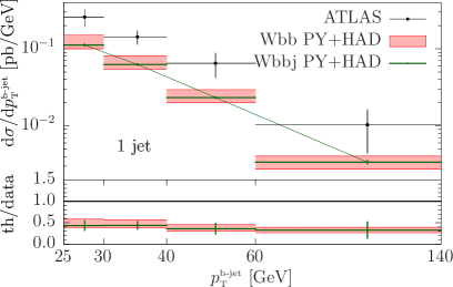
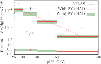
Figure 15: Transverse-momentum distribution of the $b$-tagged jet in the “1 jet” sample. The theoretical results are at the shower+hadron level. No DPI corrections included.

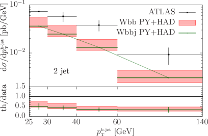
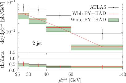
Figure 16: Transverse-momentum distribution of the $b$-tagged jet in the “2 jet” sample. The theoretical results are at the shower+hadron level. No DPI corrections included.

The ATLAS Collaboration has also measured the $p_{\mathchoice{\displaystyle}{\scriptstyle}{\scriptscriptstyle}{\scriptscriptstyle}\rm T}$ spectrum of the $b$-tagged jet in the “1 jet” and “2 jet” samples. We plot the measured values and our theoretical results in figs. 15 and 16. No DPI corrections are available for these quantities, and this partially explains the discrepancy between theory and data, both with the Wbb and Wbbj+MiNLO generator.

5.1 A different scale choice

All the results presented so far have been computed at the scales illustrated in sec. 3.1. In this section, we show a few results at the same scale used by the ATLAS Collaboration in ref. [55], where the measured cross sections are compared with the predictions of mixed 4- and 5-flavour NLO calculations [9, 10, 11], computed using MCFM [56]. The results are generated using the following central renormalization and factorization dynamical scale

$$\mu_{\mathchoice{\displaystyle}{\scriptstyle}{\scriptscriptstyle}{\scriptscriptstyle}\rm F}^{2}=\mu_{\mathchoice{\displaystyle}{\scriptstyle}{\scriptscriptstyle}{\scriptscriptstyle}\rm R}^{2}=\mu^{2}=m^{2}_{\mathchoice{\displaystyle}{\scriptstyle}{\scriptscriptstyle}{\scriptscriptstyle}\rm e\nu}+\left(p_{\mathchoice{\displaystyle}{\scriptstyle}{\scriptscriptstyle}{\scriptscriptstyle}\rm T}^{\mathchoice{\displaystyle}{\scriptstyle}{\scriptscriptstyle}{\scriptscriptstyle}\rm e\nu}\right)^{2}+\frac{m_{\scriptscriptstyle\rm b}^{2}+\left(p_{\mathchoice{\displaystyle}{\scriptstyle}{\scriptscriptstyle}{\scriptscriptstyle}\rm T}^{\mathchoice{\displaystyle}{\scriptstyle}{\scriptscriptstyle}{\scriptscriptstyle}\rm b}\right)^{2}}{2}+\frac{m_{\scriptscriptstyle\rm b}^{2}+\left(p_{\mathchoice{\displaystyle}{\scriptstyle}{\scriptscriptstyle}{\scriptscriptstyle}\rm T}^{\mathchoice{\displaystyle}{\scriptstyle}{\scriptscriptstyle}{\scriptscriptstyle}\rm\bar{b}}\right)^{2}}{2}\,.$$ (17)

The scale-variation bands computed in ref. [55] are obtained by varying $\mu$ between a quarter and four times the central value, while in our results we have varied the scales independently as discussed in sec. 4.2.

	MCFM NLO	LHE	PY+SWR	MCFM+HAD	PY+HAD
—“1 jet”	$2.16\,^{+0.78}_{-0.59}$	$2.54\,^{+0.27}_{-0.41}$	$2.39\,^{+0.23}_{-0.37}$	$1.99\,^{+0.72}_{-0.54}$	$2.40\,^{+0.22}_{-0.37}$
—“2 jet”	$1.43\,^{+0.42}_{-0.24}$	$1.52\,^{+0.38}_{-0.30}$	$1.24\,^{+0.31}_{-0.25}$	$1.37\,^{+0.40}_{-0.23}$	$1.27\,^{+0.31}_{-0.25}$

Table 2: Cross sections (in pb) for the “1 jet” and “2 jet” sample, as defined in the text, computed at fixed next-to-leading order with MCFM (second column), at the LHE by the POWHEG BOX (third column), LHE + shower effects (fourth column), MCFM corrected for hadronization effects (fifth column) and LHE + shower and hadronization (last column). Scale-variation bands are also shown.

In tab. 2 we compare the MCFM results computed by the ATLAS Collaboration with our results at different stages. The MCFM NLO results are as obtained by simply running the MCFM code, i.e. we have subtracted all the DPI corrections and undone the hadronization corrections applied by ATLAS. In this way, we can compare the results for the MCFM NLO $W$+1$b$-jet and $W$+1$b$+1$j$ production with the LHE and LHE + shower ones. We observe a good level of agreement among these predictions, within the scale-variation bands. In addition, we notice that hadronization effects (last column of the table) have a very small impact on the showered results, at the level of a few percent.

The theoretical result for “1+2 jet” production with hadronization effects included (i.e. the sum of the numbers in the MCFM+HAD column), plus DPI corrections, quoted in ref. [55], is given by

$$\sigma({\rm\mbox{1+2~{}jet}})=4.70\,^{+0.82}_{-0.65}~{}{\rm pb}\,.$$ (18)

This value for the cross section is in agreement, within the scale-variation band, with our 4-flavour result obtained with the Wbbj+MiNLO generator of eq. (14).

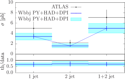
Figure 17: Cross sections, within the cuts described in the text, for the ATLAS measurement of “1 jet”, “2 jet” and “1+2 jet” $Wb$ production, using the scale of eq. (17) as central scale of the primary process. The theoretical central results and error bands have been corrected for the DPI effects of tab. 1. Results are at the full shower+hadron level.

If instead we use the scale in eq. (17) as central scale for the primary process, we get

$$\sigma({\rm\mbox{1+2~{}jet}})=5.00\,^{+0.97}_{-0.93}~{}{\rm pb}\,,$$ (19)

with all the other results for the “1 jet” and “2 jet” sample collected in fig. 17. In this figure, the cross sections obtained using eq. (17) as scale for the primary process are displayed in blue, with the associated statistical and DPI error bars. The bands are obtained exactly as in the previous section, by varying the scales around the central one. With this scale choice, we have a higher degree of overlapping of the variation bands with the data, even if the agreement is still not perfect.

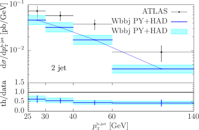
Figure 18: Transverse-momentum distribution of the $b$-tagged jet in the “1 jet” and “2 jet” samples, using the scale of eq. (17) as central scale of the primary process. The theoretical results are at the shower+hadron level. No DPI corrections included.

In fig. 18, we plot the $p_{\mathchoice{\displaystyle}{\scriptstyle}{\scriptscriptstyle}{\scriptscriptstyle}\rm T}$ spectrum of the $b$-tagged jet in the “1 jet” and “2 jet” samples. The two panels of the figure are equivalent to figs. 15 and 16, right panels, but with the scales of eq. (17). Although the blue curves are 10-20% higher than the green ones in figs. 15 and 16, the ratio of the theoretical predictions over the data is around the 50% level. We recall again that DPI corrections have not been included in these figures, and this partially accounts for the discrepancy between theoretical results and data.

6 Conclusions

The production of a $W$ boson in association with one or more $b$ jets is a significant background for $HW$ production, with the Higgs boson decaying into $b$ quarks, and to single-top and top-pair production in the Standard Model and to many new-physics searches.

In this paper we have presented a NLO+parton-shower event generator for $Wb\bar{b}j$ production, where bottom-quark mass effects and spin correlations of the leptonic decay products of the $W$ boson have been fully taken into account. The code has been automatically generated using the two available interfaces of MadGraph4 and GoSam to the POWHEG BOX.

We have applied the MiNLO procedure to this process and compared several relevant distributions with the corresponding ones generated with the NLO+parton-shower code for $Wb\bar{b}$ production. We have investigated in detail the kinematic region where the transverse momentum of the hardest jet $j$ in $Wb\bar{b}j$ production becomes small, and we have found good agreement between the two codes.

We have shown results using a dynamical scale both for the Wbb and Wbbj generators, and studied their factorization- and renormalization-scale dependence. We have compared our results with all the experimental data collected at the LHC for $Wb(b)$ production, published in the literature up to now. While we found a very good agreement with the $Wb\bar{b}$ cross section measured by the CMS Collaboration, the agreement with the ATLAS data for $Wb$ production is less satisfactory, for both our scale choices. We point out that the errors on the measurements are still quite large, and more precise results expected from the runs at higher energies will be of help in understanding the quality of the theoretical predictions.

The code for $Wb\bar{b}j$ production is available in the POWHEG BOX V2 package, under the User-Processes-V2/Wbbj/ directory, while the code for $Wb\bar{b}$ production is available in the User-Processes-V2/Wbb_dec/ folder. All the information can be found at the POWHEG BOX web page http://powhegbox.mib.infn.it.

Appendix A The change of the renormalization scheme

Our calculation was carried out in the mixed renormalization scheme (also called decoupling scheme) of ref. [36], in which the light flavours $n_{\rm lf}$ (4 in our process) are subtracted in the $\overline{\rm MS}$ scheme, while the heavy-flavour loops are subtracted at zero momentum. In this scheme the heavy flavour decouples at low energy. In fact, convergent heavy-flavour loops are suppressed by powers of the mass of the heavy flavour. The only unsuppressed contributions come from divergent graphs. But those are subtracted at zero external momenta, so their contribution is removed by renormalization for small momenta (see also ref. [57]).

A.1 The strong coupling constant

In order to make contact between the renormalization carried out in the decoupling and in the ${\overline{\rm MS}}$ scheme, we need to express the strong coupling constant $\alpha_{\mathchoice{\displaystyle}{\scriptstyle}{\scriptscriptstyle}{\scriptscriptstyle}\rm S}^{\rm(n_{\rm lf})}(\mu_{\mathchoice{\displaystyle}{\scriptstyle}{\scriptscriptstyle}{\scriptscriptstyle}\rm R})$ in the mixed scheme at the scale $\mu_{\mathchoice{\displaystyle}{\scriptstyle}{\scriptscriptstyle}{\scriptscriptstyle}\rm R}$, with $n_{\rm lf}$ light flavours, in terms of $\alpha_{\mathchoice{\displaystyle}{\scriptstyle}{\scriptscriptstyle}{\scriptscriptstyle}\rm S}^{\rm(n_{\rm f})}(\mu_{\mathchoice{\displaystyle}{\scriptstyle}{\scriptscriptstyle}{\scriptscriptstyle}\rm R})$ of the ${\overline{\rm MS}}$ scheme, with $n_{\rm f}$ light flavours.

In the mixed scheme, charge renormalization is performed at one loop with the substitution

$$\alpha_{\mathchoice{\displaystyle}{\scriptstyle}{\scriptscriptstyle}{\scriptscriptstyle}\rm S}^{b}=\mu^{2\epsilon}\,\alpha_{\mathchoice{\displaystyle}{\scriptstyle}{\scriptscriptstyle}{\scriptscriptstyle}\rm S}^{\rm(n_{\rm lf})}(\mu_{\mathchoice{\displaystyle}{\scriptstyle}{\scriptscriptstyle}{\scriptscriptstyle}\rm R})\left\{1-\alpha_{\mathchoice{\displaystyle}{\scriptstyle}{\scriptscriptstyle}{\scriptscriptstyle}\rm S}^{\rm(n_{\rm lf})}(\mu_{\mathchoice{\displaystyle}{\scriptstyle}{\scriptscriptstyle}{\scriptscriptstyle}\rm R})\,\frac{1}{\bar{\epsilon}}\left[b_{0}^{(n_{\rm lf})}-\left(\frac{\mu_{\mathchoice{\displaystyle}{\scriptstyle}{\scriptscriptstyle}{\scriptscriptstyle}\rm R}^{2}}{m^{2}}\right)^{\epsilon}\frac{T_{\mathchoice{\displaystyle}{\scriptstyle}{\scriptscriptstyle}{\scriptscriptstyle}\rm F}}{3\pi}\right]+{\cal O}\left(\alpha_{\mathchoice{\displaystyle}{\scriptstyle}{\scriptscriptstyle}{\scriptscriptstyle}\rm S}^{2}\right)\right\},$$ (20)

where $\alpha_{\mathchoice{\displaystyle}{\scriptstyle}{\scriptscriptstyle}{\scriptscriptstyle}\rm S}^{b}$ is the bare coupling constant,

$$b_{0}^{(n)}=\frac{11C_{\mathchoice{\displaystyle}{\scriptstyle}{\scriptscriptstyle}{\scriptscriptstyle}\rm A}-4\,T_{\mathchoice{\displaystyle}{\scriptstyle}{\scriptscriptstyle}{\scriptscriptstyle}\rm F}\,n}{12\pi}\,,$$ (21)

and

$$\frac{1}{\bar{\epsilon}}=\frac{1}{\epsilon}+\log(4\pi)-\gamma_{E}\,,$$ (22)

where dimensional regularization in $d=4-2\epsilon$ has been used. In the $\overline{\rm MS}$ scheme the renormalization prescription is

$$\alpha_{\mathchoice{\displaystyle}{\scriptstyle}{\scriptscriptstyle}{\scriptscriptstyle}\rm S}^{b}=\mu_{\mathchoice{\displaystyle}{\scriptstyle}{\scriptscriptstyle}{\scriptscriptstyle}\rm R}^{2\epsilon}\,\alpha_{\mathchoice{\displaystyle}{\scriptstyle}{\scriptscriptstyle}{\scriptscriptstyle}\rm S}^{\rm(n_{\rm f})}(\mu_{\mathchoice{\displaystyle}{\scriptstyle}{\scriptscriptstyle}{\scriptscriptstyle}\rm R})\left\{1-\alpha_{\mathchoice{\displaystyle}{\scriptstyle}{\scriptscriptstyle}{\scriptscriptstyle}\rm S}^{\rm(n_{\rm f})}(\mu_{\mathchoice{\displaystyle}{\scriptstyle}{\scriptscriptstyle}{\scriptscriptstyle}\rm R})\,\frac{1}{\bar{\epsilon}}\,b_{0}^{(n_{\rm f})}+{\cal O}\left(\alpha_{\mathchoice{\displaystyle}{\scriptstyle}{\scriptscriptstyle}{\scriptscriptstyle}\rm S}^{2}\right)\right\},$$ (23)

where $n_{\rm f}=n_{\rm lf}+1$.

It is straightforward to check that the couplings in the two schemes obey the well-known $n_{\rm lf}$-flavour and $n_{\rm f}$-flavour renormalization-group equation respectively

$$\frac{\mathrm{d}\alpha_{\mathchoice{\displaystyle}{\scriptstyle}{\scriptscriptstyle}{\scriptscriptstyle}\rm S}^{\rm(n_{\rm lf})}(\mu_{\mathchoice{\displaystyle}{\scriptstyle}{\scriptscriptstyle}{\scriptscriptstyle}\rm R})}{\mathrm{d}\log\mu_{\mathchoice{\displaystyle}{\scriptstyle}{\scriptscriptstyle}{\scriptscriptstyle}\rm R}^{2}} = -b_{0}^{(n_{\rm lf})}\left(\alpha_{\mathchoice{\displaystyle}{\scriptstyle}{\scriptscriptstyle}{\scriptscriptstyle}\rm S}^{\rm(n_{\rm lf})}(\mu_{\mathchoice{\displaystyle}{\scriptstyle}{\scriptscriptstyle}{\scriptscriptstyle}\rm R})\right)^{2}+{\cal O}\left(\alpha_{\mathchoice{\displaystyle}{\scriptstyle}{\scriptscriptstyle}{\scriptscriptstyle}\rm S}^{3}\right),$$ (24)

$$\frac{\mathrm{d}\alpha_{\mathchoice{\displaystyle}{\scriptstyle}{\scriptscriptstyle}{\scriptscriptstyle}\rm S}^{\rm(n_{\rm f})}(\mu_{\mathchoice{\displaystyle}{\scriptstyle}{\scriptscriptstyle}{\scriptscriptstyle}\rm R})}{\mathrm{d}\log\mu_{\mathchoice{\displaystyle}{\scriptstyle}{\scriptscriptstyle}{\scriptscriptstyle}\rm R}^{2}} = -b_{0}^{(n_{\rm f})}\left(\alpha_{\mathchoice{\displaystyle}{\scriptstyle}{\scriptscriptstyle}{\scriptscriptstyle}\rm S}^{\rm(n_{\rm f})}(\mu_{\mathchoice{\displaystyle}{\scriptstyle}{\scriptscriptstyle}{\scriptscriptstyle}\rm R})\right)^{2}+{\cal O}\left(\alpha_{\mathchoice{\displaystyle}{\scriptstyle}{\scriptscriptstyle}{\scriptscriptstyle}\rm S}^{3}\right),$$ (25)

that can be easily derived by imposing the independence of the bare coupling $\alpha_{\mathchoice{\displaystyle}{\scriptstyle}{\scriptscriptstyle}{\scriptscriptstyle}\rm S}^{b}$ under a renormalization-group transformation. Up to order $\alpha_{\mathchoice{\displaystyle}{\scriptstyle}{\scriptscriptstyle}{\scriptscriptstyle}\rm S}^{3}$, the solutions of eqs. (24) and (25) are given by

$$\alpha_{\mathchoice{\displaystyle}{\scriptstyle}{\scriptscriptstyle}{\scriptscriptstyle}\rm S}^{\rm(n_{\rm lf})}(\mu_{\mathchoice{\displaystyle}{\scriptstyle}{\scriptscriptstyle}{\scriptscriptstyle}\rm R}) = \alpha_{\mathchoice{\displaystyle}{\scriptstyle}{\scriptscriptstyle}{\scriptscriptstyle}\rm S}^{\rm(n_{\rm lf})}(m)-b_{0}^{(n_{\rm lf})}\alpha_{\mathchoice{\displaystyle}{\scriptstyle}{\scriptscriptstyle}{\scriptscriptstyle}\rm S}^{2}\log\frac{\mu_{\mathchoice{\displaystyle}{\scriptstyle}{\scriptscriptstyle}{\scriptscriptstyle}\rm R}^{2}}{m^{2}}\,,$$ (26)

$$\alpha_{\mathchoice{\displaystyle}{\scriptstyle}{\scriptscriptstyle}{\scriptscriptstyle}\rm S}^{\rm(n_{\rm f})}(\mu_{\mathchoice{\displaystyle}{\scriptstyle}{\scriptscriptstyle}{\scriptscriptstyle}\rm R}) = \alpha_{\mathchoice{\displaystyle}{\scriptstyle}{\scriptscriptstyle}{\scriptscriptstyle}\rm S}^{\rm(n_{\rm f})}(m)-b_{0}^{(n_{\rm f})}\alpha_{\mathchoice{\displaystyle}{\scriptstyle}{\scriptscriptstyle}{\scriptscriptstyle}\rm S}^{2}\log\frac{\mu_{\mathchoice{\displaystyle}{\scriptstyle}{\scriptscriptstyle}{\scriptscriptstyle}\rm R}^{2}}{m^{2}}\,.$$ (27)

Combining eqs. (20) and (23) we have

$$\alpha_{\mathchoice{\displaystyle}{\scriptstyle}{\scriptscriptstyle}{\scriptscriptstyle}\rm S}^{\rm(n_{\rm lf})}(\mu_{\mathchoice{\displaystyle}{\scriptstyle}{\scriptscriptstyle}{\scriptscriptstyle}\rm R})=\alpha_{\mathchoice{\displaystyle}{\scriptstyle}{\scriptscriptstyle}{\scriptscriptstyle}\rm S}^{\rm(n_{\rm f})}(\mu_{\mathchoice{\displaystyle}{\scriptstyle}{\scriptscriptstyle}{\scriptscriptstyle}\rm R})-\frac{2}{3}\,T_{\mathchoice{\displaystyle}{\scriptstyle}{\scriptscriptstyle}{\scriptscriptstyle}\rm F}\,\frac{\alpha_{\mathchoice{\displaystyle}{\scriptstyle}{\scriptscriptstyle}{\scriptscriptstyle}\rm S}^{2}}{2\pi}\,\log\frac{\mu_{\mathchoice{\displaystyle}{\scriptstyle}{\scriptscriptstyle}{\scriptscriptstyle}\rm R}^{2}}{m^{2}}+{\cal O}\left(\alpha_{\mathchoice{\displaystyle}{\scriptstyle}{\scriptscriptstyle}{\scriptscriptstyle}\rm S}^{3}\right)\,,$$ (28)

which is the standard $\overline{\rm MS}$ matching condition for flavour crossing

$$\alpha_{\mathchoice{\displaystyle}{\scriptstyle}{\scriptscriptstyle}{\scriptscriptstyle}\rm S}^{\rm(n_{\rm lf})}(m)=\alpha_{\mathchoice{\displaystyle}{\scriptstyle}{\scriptscriptstyle}{\scriptscriptstyle}\rm S}^{\rm(n_{\rm f})}(m)+{\cal O}\left(\alpha_{\mathchoice{\displaystyle}{\scriptstyle}{\scriptscriptstyle}{\scriptscriptstyle}\rm S}^{3}\right)\,.$$ (29)

A.2 The parton distribution functions

Similarly to what has been done for the strong coupling constant, we need to find the changes to apply to the pdfs, in order to change scheme. The parton distribution functions $f_{i}(x,\mu_{\mathchoice{\displaystyle}{\scriptstyle}{\scriptscriptstyle}{\scriptscriptstyle}\rm F})$ for $n_{\rm f}$ and $n_{\rm lf}$ massless flavours must match at the mass $m$ of the heavy quark [58], i.e. when $\mu_{\mathchoice{\displaystyle}{\scriptstyle}{\scriptscriptstyle}{\scriptscriptstyle}\rm F}=m$. More specifically, in the $\overline{\rm MS}$ subtraction scheme, they must satisfy the following (see ref. [37] for more details)

$$f^{(n_{\rm f})}_{i}(x,m) = f^{(n_{\rm lf})}_{i}(x,m)\,,\quad{\rm for\ }i\neq h\,,$$ (30)

$$f^{(n_{\rm f})}_{h}(x,m) = 0\,,$$ (31)

$$f^{(n_{\rm f})}_{\bar{h}}(x,m) = 0\,,$$ (32)

where $h$ stands for the heavy flavour. Using the Altarelli–Parisi evolution equations together with the matching conditions given in eqs. (30)-(32), one can easily find the appropriate relations between the parton densities with $n_{\rm lf}$ and $n_{\rm f}$ active flavours for $\mu$ of the order of $m$.

In fact, the Altarelli–Parisi equations for the parton densities with $n_{\rm f}=n_{\rm lf}+1$ flavours are given by

$$\frac{\partial f^{(n_{\rm f})}_{i}(x,\mu)}{\partial\log\mu^{2}}=\frac{\alpha_{\mathchoice{\displaystyle}{\scriptstyle}{\scriptscriptstyle}{\scriptscriptstyle}\rm S}^{(n_{\rm f})}(\mu)}{2\pi}\sum_{j}\int^{1}_{x}\frac{\mathrm{d}z}{z}\,f^{(n_{\rm f})}_{j}\left(\frac{x}{z},\mu\right)P^{(n_{\rm f})}_{ij}(z)\,.$$ (33)

Integrating both sides of this equation between $m$ and $\mu_{\mathchoice{\displaystyle}{\scriptstyle}{\scriptscriptstyle}{\scriptscriptstyle}\rm F}$, neglecting terms of order $\alpha_{\mathchoice{\displaystyle}{\scriptstyle}{\scriptscriptstyle}{\scriptscriptstyle}\rm S}^{2}$, and using eq. (27), we get

$$f^{(n_{\rm f})}_{i}(x,\mu_{\mathchoice{\displaystyle}{\scriptstyle}{\scriptscriptstyle}{\scriptscriptstyle}\rm F})-f^{(n_{\rm f})}_{i}(x,m)=\frac{\alpha_{\mathchoice{\displaystyle}{\scriptstyle}{\scriptscriptstyle}{\scriptscriptstyle}\rm S}^{(n_{\rm f})}(m)}{2\pi}\log\frac{\mu_{\mathchoice{\displaystyle}{\scriptstyle}{\scriptscriptstyle}{\scriptscriptstyle}\rm F}^{2}}{m^{2}}\sum_{j}\int^{1}_{x}\frac{\mathrm{d}z}{z}f^{(n_{\rm f})}_{j}\left(\frac{x}{z},m\right)P^{(n_{\rm f})}_{ij}(z)\,.$$ (34)

Since the heavy-quark parton distribution functions vanish at $\mu_{\mathchoice{\displaystyle}{\scriptstyle}{\scriptscriptstyle}{\scriptscriptstyle}\rm F}=m$ (see eqs. (31) and (32)), we can exclude them, by putting $j\neq h,\bar{h}$ in the sum, and we can write

$$f^{(n_{\rm f})}_{i}(x,\mu_{\mathchoice{\displaystyle}{\scriptstyle}{\scriptscriptstyle}{\scriptscriptstyle}\rm F})=f^{(n_{\rm f})}_{i}(x,m)+\frac{\alpha_{\mathchoice{\displaystyle}{\scriptstyle}{\scriptscriptstyle}{\scriptscriptstyle}\rm S}^{(n_{\rm f})}(m)}{2\pi}\log\frac{\mu_{\mathchoice{\displaystyle}{\scriptstyle}{\scriptscriptstyle}{\scriptscriptstyle}\rm F}^{2}}{m^{2}}\sum_{j\neq h,\bar{h}}\int^{1}_{x}\frac{\mathrm{d}z}{z}f^{(n_{\rm f})}_{j}\left(\frac{x}{z},m\right)P^{(n_{\rm f})}_{ij}(z)\,.$$ (35)

For $i=h$ (or $i=\bar{h}$), eqs. (31), (32) and (35) yield

$$f^{(n_{\rm f})}_{h}(x,\mu_{\mathchoice{\displaystyle}{\scriptstyle}{\scriptscriptstyle}{\scriptscriptstyle}\rm F})=\frac{\alpha_{\mathchoice{\displaystyle}{\scriptstyle}{\scriptscriptstyle}{\scriptscriptstyle}\rm S}^{(n_{\rm f})}(m)}{2\pi}\log\frac{\mu_{\mathchoice{\displaystyle}{\scriptstyle}{\scriptscriptstyle}{\scriptscriptstyle}\rm F}^{2}}{m^{2}}\sum_{j\neq h,\bar{h}}\int^{1}_{x}\frac{\mathrm{d}z}{z}f^{(n_{\rm f})}_{j}\left(\frac{x}{z},m\right)P^{(n_{\rm f})}_{hj}(z)\,,$$ (36)

which shows that the heavy-quark pdf is of order $\alpha_{\mathchoice{\displaystyle}{\scriptstyle}{\scriptscriptstyle}{\scriptscriptstyle}\rm S}$. Since an equation similar to eq. (35) holds for $n_{\rm lf}$ flavours

$$f^{(n_{\rm lf})}_{i}(x,\mu_{\mathchoice{\displaystyle}{\scriptstyle}{\scriptscriptstyle}{\scriptscriptstyle}\rm F})=f^{(n_{\rm lf})}_{i}(x,m)+\frac{\alpha_{\mathchoice{\displaystyle}{\scriptstyle}{\scriptscriptstyle}{\scriptscriptstyle}\rm S}^{(n_{\rm lf})}(m)}{2\pi}\log\frac{\mu_{\mathchoice{\displaystyle}{\scriptstyle}{\scriptscriptstyle}{\scriptscriptstyle}\rm F}^{2}}{m^{2}}\sum_{j\neq h,\bar{h}}\int^{1}_{x}\frac{\mathrm{d}z}{z}f^{(n_{\rm lf})}_{j}\left(\frac{x}{z},m\right)P^{(n_{\rm lf})}_{ij}(z)\,,$$ (37)

we can take the difference between eqs. (35) and (37), and using eqs. (30) and (29), we obtain, for ${i\neq h,\bar{h}}$

$$f^{(n_{\rm f})}_{i}(x,\mu_{\mathchoice{\displaystyle}{\scriptstyle}{\scriptscriptstyle}{\scriptscriptstyle}\rm F})-f^{(n_{\rm lf})}_{i}(x,\mu_{\mathchoice{\displaystyle}{\scriptstyle}{\scriptscriptstyle}{\scriptscriptstyle}\rm F})=$$

$$\qquad\qquad=\frac{\alpha_{\mathchoice{\displaystyle}{\scriptstyle}{\scriptscriptstyle}{\scriptscriptstyle}\rm S}^{(n_{\rm lf})}(m)}{2\pi}\log\frac{\mu_{\mathchoice{\displaystyle}{\scriptstyle}{\scriptscriptstyle}{\scriptscriptstyle}\rm F}^{2}}{m^{2}}\sum_{j\neq h,\bar{h}}\int^{1}_{x}\frac{\mathrm{d}z}{z}f^{(n_{\rm lf})}_{j}\left(\frac{x}{z},m\right)\left[P^{(n_{\rm f})}_{ij}(z)-P^{(n_{\rm lf})}_{ij}(z)\right]\!.\phantom{aaaa}$$ (38)

The only splitting function that depends explicitly upon the number of light flavours is the gluon splitting function, so that

$$P^{(n_{\rm f})}_{gg}(z)-P^{(n_{\rm lf})}_{gg}(z)=-\frac{2}{3}\,T_{\mathchoice{\displaystyle}{\scriptstyle}{\scriptscriptstyle}{\scriptscriptstyle}\rm F}\,\delta(1-z)\,,$$ (39)

which applied to eq. (A.2) gives

$$f^{(n_{\rm f})}_{g}(x,\mu_{\mathchoice{\displaystyle}{\scriptstyle}{\scriptscriptstyle}{\scriptscriptstyle}\rm F})-f^{(n_{\rm lf})}_{g}(x,\mu_{\mathchoice{\displaystyle}{\scriptstyle}{\scriptscriptstyle}{\scriptscriptstyle}\rm F})=-\frac{2}{3}\,T_{\mathchoice{\displaystyle}{\scriptstyle}{\scriptscriptstyle}{\scriptscriptstyle}\rm F}\,\frac{\alpha_{\mathchoice{\displaystyle}{\scriptstyle}{\scriptscriptstyle}{\scriptscriptstyle}\rm S}^{(n_{\rm lf})}(m)}{2\pi}\log\frac{\mu_{\mathchoice{\displaystyle}{\scriptstyle}{\scriptscriptstyle}{\scriptscriptstyle}\rm F}^{2}}{m^{2}}\,f^{(n_{\rm lf})}_{g}(x,m)\,.$$ (40)

The final results are then

$$f^{(n_{\rm f})}_{h\,(\bar{h})}(x,\mu_{\mathchoice{\displaystyle}{\scriptstyle}{\scriptscriptstyle}{\scriptscriptstyle}\rm F}) = {\cal O}\left(\alpha_{\mathchoice{\displaystyle}{\scriptstyle}{\scriptscriptstyle}{\scriptscriptstyle}\rm S}\right)$$ (41)

$$f^{(n_{\rm f})}_{j}(x,\mu_{\mathchoice{\displaystyle}{\scriptstyle}{\scriptscriptstyle}{\scriptscriptstyle}\rm F}) = f^{(n_{\rm lf})}_{j}(x,\mu_{\mathchoice{\displaystyle}{\scriptstyle}{\scriptscriptstyle}{\scriptscriptstyle}\rm F})+{\cal O}\left(\alpha_{\mathchoice{\displaystyle}{\scriptstyle}{\scriptscriptstyle}{\scriptscriptstyle}\rm S}^{2}\right)\,,\quad{\rm for\ }j\neq h,\bar{h},g$$ (42)

$$f^{(n_{\rm f})}_{g}(x,\mu_{\mathchoice{\displaystyle}{\scriptstyle}{\scriptscriptstyle}{\scriptscriptstyle}\rm F}) = f^{(n_{\rm lf})}_{g}(x,\mu_{\mathchoice{\displaystyle}{\scriptstyle}{\scriptscriptstyle}{\scriptscriptstyle}\rm F})\left[1-\frac{2}{3}T_{\mathchoice{\displaystyle}{\scriptstyle}{\scriptscriptstyle}{\scriptscriptstyle}\rm F}\frac{\alpha_{\mathchoice{\displaystyle}{\scriptstyle}{\scriptscriptstyle}{\scriptscriptstyle}\rm S}}{2\pi}\log\frac{\mu_{\mathchoice{\displaystyle}{\scriptstyle}{\scriptscriptstyle}{\scriptscriptstyle}\rm F}^{2}}{m^{2}}\right]+{\cal O}\left(\alpha_{\mathchoice{\displaystyle}{\scriptstyle}{\scriptscriptstyle}{\scriptscriptstyle}\rm S}^{2}\right).$$ (43)

A.3 Summarizing

We have now all the ingredients to translate our formulae for $Wb\bar{b}j$ production computed in the decoupling scheme to the standard $\overline{\rm MS}$ scheme. At the Born level, we have contributions coming from two-quark initial states and a quark-gluon initial state. We can then schematically write the contributions to the Born cross section as

$$\sigma_{qq}^{\mathchoice{\displaystyle}{\scriptstyle}{\scriptscriptstyle}{\scriptscriptstyle}\rm B} = f^{(n_{\rm lf})}_{q}(x_{1},\mu_{\mathchoice{\displaystyle}{\scriptstyle}{\scriptscriptstyle}{\scriptscriptstyle}\rm F})\,f^{(n_{\rm lf})}_{q}(x_{2},\mu_{\mathchoice{\displaystyle}{\scriptstyle}{\scriptscriptstyle}{\scriptscriptstyle}\rm F})\left[\alpha_{\mathchoice{\displaystyle}{\scriptstyle}{\scriptscriptstyle}{\scriptscriptstyle}\rm S}^{(n_{\rm lf})}(\mu_{\mathchoice{\displaystyle}{\scriptstyle}{\scriptscriptstyle}{\scriptscriptstyle}\rm R})\right]^{3}{\cal B}_{qq}\,,$$ (44)

$$\sigma_{qg}^{\mathchoice{\displaystyle}{\scriptstyle}{\scriptscriptstyle}{\scriptscriptstyle}\rm B} = f^{(n_{\rm lf})}_{q}(x_{1},\mu_{\mathchoice{\displaystyle}{\scriptstyle}{\scriptscriptstyle}{\scriptscriptstyle}\rm F})\,f^{(n_{\rm lf})}_{g}(x_{2},\mu_{\mathchoice{\displaystyle}{\scriptstyle}{\scriptscriptstyle}{\scriptscriptstyle}\rm F})\left[\alpha_{\mathchoice{\displaystyle}{\scriptstyle}{\scriptscriptstyle}{\scriptscriptstyle}\rm S}^{(n_{\rm lf})}(\mu_{\mathchoice{\displaystyle}{\scriptstyle}{\scriptscriptstyle}{\scriptscriptstyle}\rm R})\right]^{3}{\cal B}_{qg}\,,$$ (45)

where ${\cal B}_{qq}$ and ${\cal B}_{qg}$ are the squared Born amplitude for the $qq$ and $qg$ initial-state channels, respectively, with three powers of the strong coupling constant stripped off and put in front. By using eqs. (28), (42) and (43) we can write, up to order $\alpha_{\mathchoice{\displaystyle}{\scriptstyle}{\scriptscriptstyle}{\scriptscriptstyle}\rm S}^{4}$

$$\sigma_{qq}^{\mathchoice{\displaystyle}{\scriptstyle}{\scriptscriptstyle}{\scriptscriptstyle}\rm B} = f^{(n_{\rm f})}_{q}(x_{1},\mu_{\mathchoice{\displaystyle}{\scriptstyle}{\scriptscriptstyle}{\scriptscriptstyle}\rm F})\,f^{(n_{\rm f})}_{q}(x_{2},\mu_{\mathchoice{\displaystyle}{\scriptstyle}{\scriptscriptstyle}{\scriptscriptstyle}\rm F})\left[\alpha_{\mathchoice{\displaystyle}{\scriptstyle}{\scriptscriptstyle}{\scriptscriptstyle}\rm S}^{(n_{\rm f})}(\mu_{\mathchoice{\displaystyle}{\scriptstyle}{\scriptscriptstyle}{\scriptscriptstyle}\rm R})\right]^{3}\left[1-2\,T_{\mathchoice{\displaystyle}{\scriptstyle}{\scriptscriptstyle}{\scriptscriptstyle}\rm F}\frac{\alpha_{\mathchoice{\displaystyle}{\scriptstyle}{\scriptscriptstyle}{\scriptscriptstyle}\rm S}}{2\pi}\,\log\frac{\mu_{\mathchoice{\displaystyle}{\scriptstyle}{\scriptscriptstyle}{\scriptscriptstyle}\rm R}^{2}}{m^{2}}\right]{\cal B}_{qq}\,,$$ (46)

$$\sigma_{qg}^{\mathchoice{\displaystyle}{\scriptstyle}{\scriptscriptstyle}{\scriptscriptstyle}\rm B} = f^{(n_{\rm f})}_{q}(x_{1},\mu_{\mathchoice{\displaystyle}{\scriptstyle}{\scriptscriptstyle}{\scriptscriptstyle}\rm F})\,f^{(n_{\rm f})}_{g}(x_{2},\mu_{\mathchoice{\displaystyle}{\scriptstyle}{\scriptscriptstyle}{\scriptscriptstyle}\rm F})\left[\alpha_{\mathchoice{\displaystyle}{\scriptstyle}{\scriptscriptstyle}{\scriptscriptstyle}\rm S}^{(n_{\rm f})}(\mu_{\mathchoice{\displaystyle}{\scriptstyle}{\scriptscriptstyle}{\scriptscriptstyle}\rm R})\right]^{3}\left[1+\frac{2}{3}T_{\mathchoice{\displaystyle}{\scriptstyle}{\scriptscriptstyle}{\scriptscriptstyle}\rm F}\frac{\alpha_{\mathchoice{\displaystyle}{\scriptstyle}{\scriptscriptstyle}{\scriptscriptstyle}\rm S}}{2\pi}\log\frac{\mu_{\mathchoice{\displaystyle}{\scriptstyle}{\scriptscriptstyle}{\scriptscriptstyle}\rm F}^{2}}{m^{2}}\right]$$ (47)

$$\times\left[1-2\,T_{\mathchoice{\displaystyle}{\scriptstyle}{\scriptscriptstyle}{\scriptscriptstyle}\rm F}\frac{\alpha_{\mathchoice{\displaystyle}{\scriptstyle}{\scriptscriptstyle}{\scriptscriptstyle}\rm S}}{2\pi}\,\log\frac{\mu_{\mathchoice{\displaystyle}{\scriptstyle}{\scriptscriptstyle}{\scriptscriptstyle}\rm R}^{2}}{m^{2}}\right]{\cal B}_{qg}$$

$$= f^{(n_{\rm f})}_{q}(x_{1},\mu_{\mathchoice{\displaystyle}{\scriptstyle}{\scriptscriptstyle}{\scriptscriptstyle}\rm F})\,f^{(n_{\rm f})}_{g}(x_{2},\mu_{\mathchoice{\displaystyle}{\scriptstyle}{\scriptscriptstyle}{\scriptscriptstyle}\rm F})\left[\alpha_{\mathchoice{\displaystyle}{\scriptstyle}{\scriptscriptstyle}{\scriptscriptstyle}\rm S}^{(n_{\rm f})}(\mu_{\mathchoice{\displaystyle}{\scriptstyle}{\scriptscriptstyle}{\scriptscriptstyle}\rm R})\right]^{3}$$

$$\times\left[1+2\,T_{\mathchoice{\displaystyle}{\scriptstyle}{\scriptscriptstyle}{\scriptscriptstyle}\rm F}\frac{\alpha_{\mathchoice{\displaystyle}{\scriptstyle}{\scriptscriptstyle}{\scriptscriptstyle}\rm S}}{2\pi}\left(\frac{1}{3}\log\frac{\mu_{\mathchoice{\displaystyle}{\scriptstyle}{\scriptscriptstyle}{\scriptscriptstyle}\rm F}^{2}}{m^{2}}-\log\frac{\mu_{\mathchoice{\displaystyle}{\scriptstyle}{\scriptscriptstyle}{\scriptscriptstyle}\rm R}^{2}}{m^{2}}\right)\right]{\cal B}_{qg}\,.$$

Applying the same change of scheme to the virtual and real contributions would give corrections of order $\alpha_{\mathchoice{\displaystyle}{\scriptstyle}{\scriptscriptstyle}{\scriptscriptstyle}\rm S}^{5}$ or higher, beyond the NLO accuracy of our calculation. In summary, in order to change scheme, we have to:

• add a term

  $$-2\,T_{\mathchoice{\displaystyle}{\scriptstyle}{\scriptscriptstyle}{\scriptscriptstyle}\rm F}\,\frac{\alpha_{\mathchoice{\displaystyle}{\scriptstyle}{\scriptscriptstyle}{\scriptscriptstyle}\rm S}}{2\pi}\log\left(\frac{\mu_{\mathchoice{\displaystyle}{\scriptstyle}{\scriptscriptstyle}{\scriptscriptstyle}\rm R}^{2}}{m^{2}}\right)\,{\cal B}_{qq}$$ (48)

  to the $qq$ channel;

• add a term

  $$2\,T_{\mathchoice{\displaystyle}{\scriptstyle}{\scriptscriptstyle}{\scriptscriptstyle}\rm F}\,\frac{\alpha_{\mathchoice{\displaystyle}{\scriptstyle}{\scriptscriptstyle}{\scriptscriptstyle}\rm S}}{2\pi}\left[\frac{1}{3}\log\left(\frac{\mu_{\mathchoice{\displaystyle}{\scriptstyle}{\scriptscriptstyle}{\scriptscriptstyle}\rm F}^{2}}{m^{2}}\right)-\log\left(\frac{\mu_{\mathchoice{\displaystyle}{\scriptstyle}{\scriptscriptstyle}{\scriptscriptstyle}\rm R}^{2}}{m^{2}}\right)\right]{\cal B}_{qg}$$ (49)

  to the $qg$ channel.

References

- [1] ATLAS Collaboration Collaboration, G. Aad et. al., Observation of a new particle in the search for the Standard Model Higgs boson with the ATLAS detector at the LHC, Phys.Lett. B716 (2012) 1–29, [arXiv:1207.7214].
- [2] CMS Collaboration Collaboration, S. Chatrchyan et. al., Observation of a new boson at a mass of 125 GeV with the CMS experiment at the LHC, Phys.Lett. B716 (2012) 30–61, [arXiv:1207.7235].
- [3] F. Maltoni, G. Ridolfi, and M. Ubiali, b-initiated processes at the LHC: a reappraisal, JHEP 1207 (2012) 022, [arXiv:1203.6393].
- [4] R. K. Ellis and S. Veseli, Strong radiative corrections to production in collisions, Phys.Rev. D60 (1999) 011501, [hep-ph/9810489].
- [5] F. Febres Cordero, L. Reina, and D. Wackeroth, NLO QCD corrections to boson production with a massive -quark jet pair at the Tevatron collider, Phys.Rev. D74 (2006) 034007, [hep-ph/0606102].
- [6] F. Febres Cordero, L. Reina, and D. Wackeroth, - and -boson production with a massive bottom-quark pair at the Large Hadron Collider, Phys.Rev. D80 (2009) 034015, [arXiv:0906.1923].
- [7] S. Badger, J. M. Campbell, and R. Ellis, QCD corrections to the hadronic production of a heavy quark pair and a -boson including decay correlations, JHEP 1103 (2011) 027, [arXiv:1011.6647].
- [8] R. Frederix, S. Frixione, V. Hirschi, F. Maltoni, R. Pittau, et. al., and boson production in association with a bottom-antibottom pair, JHEP 1109 (2011) 061, [arXiv:1106.6019].
- [9] J. Campbell, R. K. Ellis, F. Maltoni, and S. Willenbrock, Production of a W boson and two jets with one b-quark tag, Phys. Rev. D75 (2007) 054015, [hep-ph/0611348].
- [10] J. Campbell, R. K. Ellis, F. Febres Cordero, F. Maltoni, L. Reina, D. Wackeroth, and S. Willenbrock, Associated production of a boson and one jet, Phys. Rev. D79 (2009) 034023, [0809.3003].
- [11] J. Campbell, F. Caola, F. Febres Cordero, L. Reina, and D. Wackeroth, NLO QCD predictions for jet and jet production with at least one jet at the 7 TeV LHC, Phys.Rev. D86 (2012) 034021, [arXiv:1107.3714].
- [12] C. Oleari and L. Reina, production in POWHEG, JHEP 1108 (2011) 061, [arXiv:1105.4488].
- [13] P. Nason, A new method for combining NLO QCD with shower Monte Carlo algorithms, JHEP 11 (2004) 040, [hep-ph/0409146].
- [14] S. Frixione, P. Nason, and C. Oleari, Matching NLO QCD computations with Parton Shower simulations: the POWHEG method, JHEP 11 (2007) 070, [arXiv:0709.2092].
- [15] S. Alioli, P. Nason, C. Oleari, and E. Re, A general framework for implementing NLO calculations in shower Monte Carlo programs: the POWHEG BOX, JHEP 06 (2010) 043, [arXiv:1002.2581].
- [16] T. Stelzer and W. F. Long, Automatic generation of tree level helicity amplitudes, Comput. Phys. Commun. 81 (1994) 357–371, [hep-ph/9401258].
- [17] J. Alwall et. al., MadGraph/MadEvent v4: The New Web Generation, JHEP 09 (2007) 028, [arXiv:0706.2334].
- [18] J. M. Campbell, R. K. Ellis, R. Frederix, P. Nason, C. Oleari, et. al., NLO Higgs Boson Production Plus One and Two Jets Using the POWHEG BOX, MadGraph4 and MCFM, JHEP 1207 (2012) 092, [arXiv:1202.5475].
- [19] G. Luisoni, P. Nason, C. Oleari, and F. Tramontano, /HZ + 0 and 1 jet at NLO with the POWHEG BOX interfaced to GoSam and their merging within MiNLO, JHEP 1310 (2013) 083, [arXiv:1306.2542].
- [20] G. Cullen, N. Greiner, G. Heinrich, G. Luisoni, P. Mastrolia, et. al., Automated One-Loop Calculations with GoSam, Eur.Phys.J. C72 (2012) 1889, [arXiv:1111.2034].
- [21] G. Cullen, H. van Deurzen, N. Greiner, G. Heinrich, G. Luisoni, et. al., GS-2.0: a tool for automated one-loop calculations within the Standard Model and beyond, Eur.Phys.J. C74 (2014), no. 8 3001, [arXiv:1404.7096].
- [22] K. Hamilton, P. Nason, and G. Zanderighi, MINLO: Multi-Scale Improved NLO, JHEP 1210 (2012) 155, [arXiv:1206.3572].
- [23] P. Nogueira, Automatic Feynman graph generation, J.Comput.Phys. 105 (1993) 279–289.
- [24] J. Kuipers, T. Ueda, J. Vermaseren, and J. Vollinga, FORM version 4.0, Comput.Phys.Commun. 184 (2013) 1453–1467, [arXiv:1203.6543].
- [25] G. Cullen, M. Koch-Janusz, and T. Reiter, Spinney: A Form Library for Helicity Spinors, Comput.Phys.Commun. 182 (2011) 2368–2387, [arXiv:1008.0803].
- [26] H. van Deurzen, G. Luisoni, P. Mastrolia, E. Mirabella, G. Ossola, et. al., Multi-leg One-loop Massive Amplitudes from Integrand Reduction via Laurent Expansion, JHEP 1403 (2014) 115, [arXiv:1312.6678].
- [27] T. Peraro, Ninja: Automated Integrand Reduction via Laurent Expansion for One-Loop Amplitudes, Comput.Phys.Commun. 185 (2014) 2771–2797, [arXiv:1403.1229].
- [28] P. Mastrolia, E. Mirabella, and T. Peraro, Integrand reduction of one-loop scattering amplitudes through Laurent series expansion, JHEP 1206 (2012) 095, [arXiv:1203.0291].
- [29] A. van Hameren, OneLOop: For the evaluation of one-loop scalar functions, Comput.Phys.Commun. 182 (2011) 2427–2438, [arXiv:1007.4716].
- [30] G. Cullen, J. P. Guillet, G. Heinrich, T. Kleinschmidt, E. Pilon, et. al., Golem95C: A library for one-loop integrals with complex masses, Comput.Phys.Commun. 182 (2011) 2276–2284, [arXiv:1101.5595].
- [31] G. Ossola, C. G. Papadopoulos, and R. Pittau, Reducing full one-loop amplitudes to scalar integrals at the integrand level, Nucl. Phys. B763 (2007) 147–169, [hep-ph/0609007].
- [32] R. K. Ellis, W. Giele, and Z. Kunszt, A Numerical Unitarity Formalism for Evaluating One-Loop Amplitudes, JHEP 0803 (2008) 003, [arXiv:0708.2398].
- [33] P. Mastrolia, G. Ossola, T. Reiter, and F. Tramontano, Scattering AMplitudes from Unitarity-based Reduction Algorithm at the Integrand-level, JHEP 1008 (2010) 080, [arXiv:1006.0710].
- [34] L. Reina and T. Schutzmeier, Towards + j at NLO with an Automatized Approach to One-Loop Computations, JHEP 1209 (2012) 119, [arXiv:1110.4438].
- [35] J. Alwall, R. Frederix, S. Frixione, V. Hirschi, F. Maltoni, et. al., The automated computation of tree-level and next-to-leading order differential cross sections, and their matching to parton shower simulations, JHEP 1407 (2014) 079, [arXiv:1405.0301].
- [36] J. C. Collins, F. Wilczek, and A. Zee, Low-Energy Manifestations of Heavy Particles: Application to the Neutral Current, Phys.Rev. D18 (1978) 242.
- [37] M. Cacciari, M. Greco, and P. Nason, The spectrum in heavy flavor hadroproduction, JHEP 9805 (1998) 007, [hep-ph/9803400].
- [38] K. Hamilton, P. Nason, C. Oleari, and G. Zanderighi, Merging H/W/Z + 0 and 1 jet at NLO with no merging scale: a path to parton shower + NNLO matching, JHEP 1305 (2013) 082, [arXiv:1212.4504].
- [39] J. M. Campbell, R. K. Ellis, P. Nason, and G. Zanderighi, W and Z bosons in association with two jets using the POWHEG method, JHEP 1308 (2013) 005, [arXiv:1303.5447].
- [40] A. Kardos, P. Nason, and C. Oleari, Three-jet production in POWHEG, JHEP 1404 (2014) 043, [arXiv:1402.4001].
- [41] L. Barzè, M. Chiesa, G. Montagna, P. Nason, O. Nicrosini, et. al., W production in hadronic collisions using the POWHEG+MiNLO method, JHEP 1412 (2014) 039, [arXiv:1408.5766].
- [42] M. Grazzini, NNLO predictions for the Higgs boson signal in the and decay channels, JHEP 0802 (2008) 043, [arXiv:0801.3232].
- [43] S. Catani, L. Cieri, G. Ferrera, D. de Florian, and M. Grazzini, Vector boson production at hadron colliders: a fully exclusive QCD calculation at NNLO, Phys.Rev.Lett. 103 (2009) 082001, [arXiv:0903.2120].
- [44] K. Hamilton, P. Nason, E. Re, and G. Zanderighi, NNLOPS simulation of Higgs boson production, JHEP 1310 (2013) 222, [arXiv:1309.0017].
- [45] K. Hamilton, P. Nason, and G. Zanderighi, Finite quark-mass effects in the NNLOPS POWHEG+MiNLO Higgs generator, arXiv:1501.0463.
- [46] A. Karlberg, E. Re, and G. Zanderighi, NNLOPS accurate Drell-Yan production, JHEP 1409 (2014) 134, [arXiv:1407.2940].
- [47] A. D. Martin, W. J. Stirling, R. S. Thorne, and G. Watt, Parton distributions for the LHC, Eur. Phys. J. C63 (2009) 189–285, [arXiv:0901.0002].
- [48] M. Cacciari, G. P. Salam, and G. Soyez, The anti- jet clustering algorithm, JHEP 04 (2008) 063, [arXiv:0802.1189].
- [49] M. Cacciari and G. P. Salam, Dispelling the myth for the jet-finder, Phys.Lett. B641 (2006) 57–61, [hep-ph/0512210].
- [50] M. Cacciari, G. P. Salam, and G. Soyez, FastJet User Manual, Eur.Phys.J. C72 (2012) 1896, [arXiv:1111.6097].
- [51] T. Sjostrand, S. Mrenna, and P. Z. Skands, PYTHIA 6.4 Physics and Manual, JHEP 0605 (2006) 026, [hep-ph/0603175].
- [52] G. Corcella et. al., HERWIG 6: An event generator for hadron emission reactions with interfering gluons (including supersymmetric processes), JHEP 01 (2001) 010, [hep-ph/0011363].
- [53] G. Corcella, I. Knowles, G. Marchesini, S. Moretti, K. Odagiri, et. al., HERWIG 6.5 release note, hep-ph/0210213.
- [54] CMS Collaboration Collaboration, S. Chatrchyan et. al., Measurement of the production cross section for a boson and two jets in collisions at TeV, Phys.Lett. B735 (2014) 204, [arXiv:1312.6608].
- [55] ATLAS Collaboration Collaboration, G. Aad et. al., Measurement of the cross-section for boson production in association with -jets in collisions at = 7 TeV with the ATLAS detector, JHEP 1306 (2013) 084, [arXiv:1302.2929].
- [56] http://mcfm.fnal.gov.
- [57] T. Appelquist and J. Carazzone, Infrared Singularities and Massive Fields, Phys.Rev. D11 (1975) 2856.
- [58] J. C. Collins and W.-K. Tung, Calculating Heavy Quark Distributions, Nucl.Phys. B278 (1986) 934.