Spectrum transformation and conservation laws of the lattice potential KdV equation

Abstract

Many multi-dimensional consistent discrete systems have soliton solutions with nonzero backgrounds, which brings difficulty in the investigation of integrable characteristics. In this letter we derive infinitely many conserved quantities for the lattice potential Korteweg-de Vries equation. The derivation is based on the fact that the scattering data $a(z)$ is independent of discrete space and time and the analytic property of Jost solutions of the discrete Schrödinger spectral problem. The obtained conserved densities are different from those in the known literatures. They are asymptotic to zero when $|n|$ (or $|m|$) tends to infinity. To obtain these results, we reconstruct a discrete Riccati equation by using a conformal map which transforms the upper complex plane to the inside of unit circle. Series solution to the Riccati equation is constructed based on the analytic and asymptotic properties of Jost solutions.

Keywords: conserved quantities, analytic properties, inverse scattering transform, conformal map, lattice potential KdV equation
PACS: 02.30.Ik, 02.30.Ik, 02.90.+p
MSC: 39-04, 39A05, 39A14

1 Introduction

For a nonlinear partial differential equation, possessing infinitely many conservation laws indicates the equation is integrable. In the fully discrete case, multi-dimensional consistency[1, 2, 3] provides a kind of strong integrability, under which and extra conditions lattice equations defined on quadrilateral were classified[3] and discrete Boussinesq(DBSQ)-type equations were found[4] as multi-component models. For these multi-dimensional consistent equations, infinitely many conservation laws were already constructed in several different ways[5, 6, 7, 8, 9, 10, 11, 12, 13, 14]. However, these known conservation laws are only formal ones — the nonzero boundary condition at infinity (asymptotic behavior) of the solutions of the considered lattice equations was neglected.

How does asymptotic behavior play roles? A discrete conservation law is defined in the form

$$(E_{m}-1)F_{n,m}=(E_{n}-1)J_{n,m},$$ (1.1)

where $E_{m}$ and $E_{n}$ are shift operators defined as $E_{m}f_{n,m}=f_{n,m+1}$ and $E_{n}f_{n,m}=f_{n+1,m}$. We request $F_{n,m}$ and $J_{n,m}$ tend to zero fast enough when $|n|\to\infty$ so that $\sum_{n=-\infty}^{\infty}[(E_{n}-1)J_{n,m}]=0$ and the sumation $\sum_{n=-\infty}^{\infty}F_{n,m}$ makes sense. As a result, $\sum_{n=-\infty}^{\infty}F_{n,m}$ is indenpendent of $m$ and represents a conserved quantity with respect to $m$.

To explain more, as an example, let us look at the lattice potential Korteweg-de Vries (lpKdV) equation[15, 16], also known as H1 equation in the Adler-Bobenko-Suris (ABS) list[3],

$$(\widehat{\widetilde{u}}-u)(\widetilde{u}-\widehat{u})=p^{2}-q^{2}~{},$$ (1.2)

where $u=u_{n,m}$, $\widetilde{u}=u_{n+1,m}$, $\widehat{u}=u_{n,m+1}$, $\widehat{\widetilde{u}}=u_{n+1,m+1}$, and lattice parameters $p$ for direction $n$ and $q$ for direction $m$ are arbitrary constants. Unlike most of continuous integrable systems, $u=0$ is not a solution to the lpKdV equation (1.2). It has a simplest solution

$$u=pn+qm+c$$ (1.3)

with a constant $c$. The $N$-soliton solution has the form[17, 18]

$$u=pn+qm+c+w$$ (1.4)

where

$$w\to 0,~{}~{}|n|\to\infty~{}(\mathrm{or}~{}|m|\to\infty).$$ (1.5)

Solution (1.3) is usually called a background of solitons. It has been known that most of members in the ABS list and DBSQ-type equations have either linear or exponential backgrounds (cf. [17, 18, 19, 20, 21, 22, 23]). The nonzero background will bring difficulties in finding convergent conserved quantities. For the lpKdV equation (1.2), due to the background (1.3), the equation itself is not in a conserved form and the discrete integral of function of $u$, for example, $\sum^{\infty}_{n=-\infty}u_{n,m}$, does not make sense because with the background (1.3) the summation is not convergent at all. With regard to discrete conservation laws, as an example, let us take a look at the second conservation law of the lpKdV equation derived from its Lax pair (cf. [12]), which is in the form (1.1) with

$$F_{n,m}=\frac{1}{(u-\widetilde{\widetilde{u}})(\widetilde{u}-\widetilde{\widetilde{\widetilde{u}}})},~{}~{}J_{n,m}=\frac{1}{(\widetilde{u}-\widehat{u})(u-\widetilde{\widetilde{u}})}.$$ (1.6)

Obviously, for $u$ defined in (1.4) with the background (1.3), neither $F_{n,m}$ nor $J_{n,m}$ is asymptotic to zero when $|n|\to 0$ or $|m|\to 0$. Although one can artificially add constants $-1/4p^{2}$ and $1/2p(p-q)$ to the above $F_{n,m}$ and $J_{n,m}$ respectively so that they get zero asymptotic behaviors, these constants can not be derived naturally. This is the drawback.

In this letter, for the lpKdV equation (1.2), we derive its infinitely many conserved quantities of which each corresponding conserved density $F_{n,m}\to 0$ when $|n|\to\infty$ and the conserved quantity $\sum^{\infty}_{n=-\infty}F_{n,m}$ is convergent. Our approach is a by-product of the inverse scattering transform (IST). In the IST, the scattering data $a(\lambda)$ (connected with the transmission coefficient $T$ by $T=1/a(\lambda)$) is time-independent and it is asymptotically related to wave functions (Jost solutions) in a certain way. $a(\lambda)$ can be expanded in the complex plane and coefficient of each term provides a conserved quantity (functional). Such an approach was first proposed by Zakharov and Shabat in [24] where they derived conserved quantities for the nonlinear Schrödinger equation. Later, it was applied to the Ablowitz-Ladik hierarchy[25]. The approach was also used to obtain conserved quantities for the KdV equation (see [26]). However, for the fully discrete multi-dimensionally consistent lpKdV equation (1.2), particularly, $u$ having non-zero background, we need to reconstruct a new discrete Riccati equation by using a conformal map which transforms the upper complex plane to the inside of unit circle. Series solution to the Riccati equation is constructed based on the analytic and asymptotic properties of Jost solutions.

The letter is organized as follows. In Sec.2 we recall some necessary results in the direct scattering problem of the lpKdV equation given in [22]. Then in Sec.3 we derive infinitely many conserved quantities for the lpKdV equation. Finally, Sec.4 is for conclusions. Besides, we will revisit solutions to the Riccati equation in Appendix.

2 Preliminary

In this section we recall some results in the IST procedure of the lpKdV equation described in [22]. These results are necessary in our approach. Throughout the paper we suppose the spacing parameters $p>0$ and $q>0$.

The lpKdV equation (1.2) has the following Lax pair

$$\left(\begin{array}[]{c}\widetilde{\phi}_{1}\\ \widetilde{\phi}_{2}\end{array}\right)=\left(\begin{array}[]{cc}-u&u\widetilde{u}+p^{2}-r^{2}\\ -1&\widetilde{u}\end{array}\right)\left(\begin{array}[]{c}\phi_{1}\\ \phi_{2}\end{array}\right),$$ (2.1g)

$$\left(\begin{array}[]{c}\widehat{\phi}_{1}\\ \widehat{\phi}_{2}\end{array}\right)=\left(\begin{array}[]{cc}-u&u\widehat{u}+q^{2}-r^{2}\\ -1&\widehat{u}\end{array}\right)\left(\begin{array}[]{c}\phi_{1}\\ \phi_{2}\end{array}\right).$$ (2.1n)

One can rewrite (2.1g) into a scalar discrete Schrödinger problem[27, 28]

$$\widetilde{\widetilde{g}}-s\,\widetilde{g}+(p^{2}+z^{2})g=0,$$ (2.2)

where

$$s=s_{n,m}=\widetilde{\widetilde{u}}-u$$ (2.3)

and we have replaced the wave function $\phi_{2}$ with $g$ and the spectral parameter $r$ with $iz$. It then follows from the structure (1.4) that

$$s\sim 2p,~{}~{}|n|\to\infty.$$ (2.4)

This is the boundary condition for $s$ or $u$, and we request $s$ falls in the space (cf.[22, 27])

$$P_{\mu}=\Bigl{\{}s_{n,m}\,:\,\sum_{n=-\infty}^{\infty}|n^{\mu}(s_{n,m}-2p)|<\infty\Bigr{\}},~{}\mu=0,1,2.$$ (2.5)

We note that in direct scattering problem $m$ is treated as a constant or zero.

Under the boundary condition (2.5), the difference spectral problem (2.2) admits Jost solutions $\varphi$ and $\psi$ with asymptotic property

$$\varphi(n;z)\sim(p-iz)^{n},~{}~{}~{}(n\to-\infty),$$ (2.6a)

$$\psi(n;z)\sim(p+iz)^{n},~{}~{}~{}(n\to\infty),$$ (2.6b)

where $\varphi(n;z)$ and $\psi(n;z)$ are analytic in the upper complex plane $\mathrm{Im}z>0$ and continuous in $\mathrm{Im}z\geq 0$. Besides,

$$\varphi(n;z)(p-iz)^{-n}\sim 1+O\Bigl{(}\frac{1}{z}\Bigr{)},~{}~{}~{}(||z||\to\infty),$$ (2.7a)

$$\psi(n;z)(p+iz)^{-n}\sim 1+O\Bigl{(}\frac{1}{z}\Bigr{)},~{}~{}~{}(||z||\to\infty).$$ (2.7b)

There is a linear relation

$$\varphi(n;z)=a(z)\psi(n;-z)+b(z)\psi(n;z),~{}~{}(z\in\mathbb{R}).$$ (2.8)

$a(z)$ is independent of $n$ and expressed as

$$a(z)=\frac{1}{2iz}\mathrm{W}_{n}[\varphi(n;z),\psi(n;z)],$$ (2.9)

where the Casorati determinant with respect to $n$ is defined as

$$\mathrm{W}_{n}[f(n),g(n)]=(p^{2}+z^{2})^{-n}\,\begin{vmatrix}f(n;z)&g(n;z)\\ f(n+1;z)&g(n+1;z)\end{vmatrix}.$$ (2.10)

Thanks to the analytic property of $\varphi$ and $\psi$, the relation (2.9) can be extended to the upper complex plane, i.e. $a(z)$ is analytic in $\mathrm{Im}z>0$. For the asymptotic property, $a(z)\sim 1$ when $||z||\to\infty$ and $a(z)$ can be expanded in the neighbourhood of $\infty$ as

$$a(z)=1+\sum^{\infty}_{j=1}\frac{\alpha_{j}}{z^{j}}.$$ (2.11)

$a(z)$ has finite zeros $\{z=i\kappa_{l}\}^{N}_{l=1}$ and due to analytic property and uniqueness, $a(z)$ can be expressed as (cf.[22])

$$a(z)=\prod^{N}_{j=1}\frac{z-i\kappa_{j}}{z+i\kappa_{j}},~{}~{}~{}~{}(\kappa_{j}>0).$$

Therefore $a(z)$ is independent of both $n$ and $m$.

3 Infinitely many conserved quantities

3.1 General scheme

Making use of the relation (2.9) and the asymptotic behavior (2.6), we have

$$a(z)\sim\frac{\varphi(n;z)}{2iz(p-iz)^{n}}\Bigl{(}p+iz-\frac{\varphi(n+1;z)}{\varphi(n;z)}\Bigr{)},~{}~{}(n\to\infty),$$ (3.1)

and consequently,

$$\ln a(z)\sim-\ln 2iz+G_{n}+B_{n},~{}~{}(n\to\infty),$$ (3.2)

where

$$G_{n}=\ln\frac{\varphi(n;z)}{(p-iz)^{n}},~{}~{}B_{n}=\ln(p+iz-\theta)$$ (3.3)

and

$$\theta=\theta(n)=\frac{\varphi(n+1;z)}{\varphi(n;z)}.$$ (3.4)

Noting that $\lim_{n\to-\infty}B_{n}=\ln 2iz$, we have

$$\ln a(z)\sim G_{n}+B_{n}-B_{-\infty},~{}~{}(n\to\infty).$$ (3.5)

Here $B_{-\infty}$ stands for $\lim_{n\to-\infty}B_{n}$ and hereafter we also employ similar notations such as $B_{\infty}$ and $G_{-\infty}$ without confusion. Next, defining

$$\Gamma_{n}=(E_{n}-1)G_{n}=\ln\frac{\theta}{p-iz}$$ (3.6)

and noting that $G_{-\infty}=0$ due to the asymptotic property (2.6a), we find

$$\ln a(z)\sim\sum^{n-1}_{j=-\infty}\Gamma_{j}+\sum^{n-1}_{j=-\infty}(B_{j+1}-B_{j}),~{}~{}(n\to\infty).$$ (3.7)

Thus, since $a(z)$ is independent of $n$ it is then recovered via

$$\ln a(z)= \lim_{n\to\infty}\Bigl{[}\sum^{n-1}_{j=-\infty}\Gamma_{j}+\sum^{n-1}_{j=-\infty}(B_{j+1}-B_{j})\Bigr{]}$$

$$= \sum^{\infty}_{n=-\infty}\ln\frac{\theta}{p-iz}+B_{\infty}-B_{-\infty}.$$ (3.8)

In principle, this will provide a set of conserved quantities $\{K_{j}\}$ by expanding

$$\ln a(z)=\ln\Bigl{(}1+\sum^{\infty}_{j=1}\frac{\alpha_{j}}{z^{j}}\Bigr{)}=\sum^{\infty}_{j=1}\frac{K_{j}}{z^{j}}.$$ (3.9)

3.2 Riccati equation and conformal map

The known discrete Riccati equation w.r.t. $\theta$ corresponding to (2.2) (with $g=\varphi(n;z)$) is[12]

$$\widetilde{\theta}\theta-s\,\theta+\varepsilon^{2}=0,~{}~{}\varepsilon^{2}=p^{2}+z^{2}.$$ (3.10)

It admits a series solution[12]

$$\theta=\frac{\varepsilon^{2}}{s}\Bigl{(}1+\sum_{j=1}^{\infty}\theta_{j}\varepsilon^{2j}\Bigr{)},$$ (3.11a)

with

$$\theta_{j+1}=\frac{1}{s\widetilde{s}}\sum_{i=0}^{j}\widetilde{\theta}_{i}\theta_{j-i},~{}~{}j=0,1,2,\cdots,~{}~{}(\theta_{0}=1),$$ (3.11b)

in which

$$\theta_{1}=\frac{1}{s\widetilde{s}},~{}~{}\theta_{2}=\frac{1}{s\widetilde{s}}\Bigl{(}\frac{1}{s\widetilde{s}}+\frac{1}{\widetilde{s}\,\widetilde{\widetilde{s}}}\Bigr{)},~{}~{}\cdots\cdots.$$ (3.12)

Obviously, with the above form (3.11) for $\theta$, it is hard to expand $\ln\frac{\theta}{p-iz}$ into a series of $z$ with negative powers which matches the expansion (3.9).

To over come this obstacle, we consider

$$\omega=\frac{\theta}{p-iz}$$ (3.13)

under which

$$\Gamma_{n}=\ln\omega,~{}~{}~{}B_{n}=\ln\Bigl{(}\frac{p+iz}{p-iz}-\omega\Bigr{)}+\ln(p-iz),$$ (3.14)

and the Riccati equation w.r.t. $\omega$ takes the form

$$\widetilde{\omega}\omega-\frac{s\,\omega}{p-iz}+\frac{p+iz}{p-iz}=0.$$ (3.15)

To solve it, we introduce a conformal map

$$\lambda=\frac{p+iz}{p-iz}$$ (3.16)

to transform the upper $z$-plane to the inside of unit circle on the $\lambda$-plane, as depicted in Fig.1.

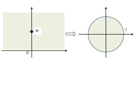
Figure 1: Conformal map (3.16)

Under this conformal map and noting that

$$z=ip\frac{1-\lambda}{1+\lambda},$$ (3.17)

(3.14) reads

$$\Gamma_{n}=\ln\omega,~{}~{}~{}B_{n}=\ln(\lambda-\omega)+\ln\frac{2p}{1+\lambda},$$ (3.18)

(3.8) reads

$$\ln a\Bigl{(}ip\frac{1-\lambda}{1+\lambda}\Bigr{)}=\sum^{\infty}_{n=-\infty}\ln\omega+B_{\infty}-B_{-\infty},$$ (3.19)

and the Riccati equation (3.15) is written as

$$\omega(\widetilde{\omega}-\widetilde{x})-\lambda\widetilde{x}\omega+\lambda=0,$$ (3.20)

where

$$x=\underaccent{\tilde}{s}/2p=(\widetilde{u}-\underaccent{\tilde}{u})/2p,$$ (3.21)

which tends to 1 as $|n|\to\infty$. (3.20) has the following solution,

$$\omega=x\Bigl{(}1+\sum_{j=1}^{\infty}\omega_{j}\lambda^{j}\Bigr{)},~{}~{}~{}(||\lambda||<1)$$ (3.22a)

with

$$\omega_{1}=1-\frac{1}{x\,\underaccent{\tilde}{x}},$$ (3.22b)

$$\omega_{2}=\Bigl{(}1-\frac{1}{\underaccent{\tilde}{x}\,\underaccent{\tilde}{\dt x}}\Bigr{)}\,\frac{1}{x\,\underaccent{\tilde}{x}},$$ (3.22c)

$$\omega_{j+1}=\underaccent{\tilde}{\omega}_{j}-\sum_{k=1}^{j}\underaccent{\tilde}{\omega}_{k}\,{\omega}_{j+1-k},~{}~{}j=2,3,\cdots.$$ (3.22d)

Noting that the fact $x\sim 1$ as $|n|\to\infty$, we immediately have the following.

Proposition 1.

All the $\{\omega_{j}\}$ defined in (3.22) are asymptotic to zero as $|n|\to\infty$.

3.3 Infinitely many conserved quantities

From now on everything is considered on $\lambda$-plane. Based on proposition 1, for the term $B_{n}$ in (3.18) we find $B_{\infty}=B_{-\infty}$, from which and (3.19) it follows that

$$\ln a\Bigl{(}ip\frac{1-\lambda}{1+\lambda}\Bigr{)}=\sum^{\infty}_{n=-\infty}\ln\omega.$$ (3.23)

Theoretically, the l.h.s. has the expansion (at the origin point of $\lambda$-plane)

$$\ln a\Bigl{(}ip\frac{1-\lambda}{1+\lambda}\Bigr{)}=H_{0}+\sum^{\infty}_{j=1}H_{j}\,\lambda^{j}$$ (3.24)

due to the property that $a\bigl{(}ip\frac{1-\lambda}{1+\lambda}\bigr{)}$ is analytic inside the unit circle, while the r.h.s. of (3.23) can be explicitly expressed as

$$\sum^{\infty}_{n=-\infty}\ln\omega= \sum^{\infty}_{n=-\infty}\ln x+\sum^{\infty}_{n=-\infty}\ln\Bigl{(}1+\sum_{j=1}^{\infty}\omega_{j}\lambda^{j}\Bigr{)}$$

$$= \sum^{\infty}_{n=-\infty}\ln x+\sum_{j=1}^{\infty}\left(\,\sum^{\infty}_{n=-\infty}h_{j}(\mathbf{\boldsymbol{\omega}})\right)\lambda^{j}.$$ (3.25)

Here, $\{h_{j}(\mathbf{\boldsymbol{\omega}})\}$, we call them $h$-polynomials for short, are the polynomials defined in the following way (cf.[12])

$$\ln\biggl{(}1+\sum_{i=1}^{\infty}\omega_{i}\lambda^{i}\biggr{)}=\sum_{j=1}^{\infty}h_{j}(\boldsymbol{\omega})\lambda^{j},$$ (3.26)

where $\boldsymbol{\omega}=(\omega_{1},\omega_{2},\cdots)$ and the first three of $\{h_{j}(\boldsymbol{\omega})\}$ are

$$h_{1}(\boldsymbol{\omega})=\omega_{1},~{}~{}h_{2}(\boldsymbol{\omega})=-\frac{1}{2}\omega_{1}^{2}+\omega_{2},~{}~{}h_{3}(\boldsymbol{\omega})=\frac{1}{3}\omega_{1}^{3}-\omega_{1}\omega_{2}+\omega_{3}.$$ (3.27)

A general description for such polynomials is given in Appendix A.

Thus, it is clear that the infinitely many conserved quantities are the following.

Proposition 2.

The infinitely many conserved densities of the lpKdV equation (1.2) are

$$H_{0}=\sum^{\infty}_{n=-\infty}\ln x,~{}~{}H_{j}=\sum^{\infty}_{n=-\infty}h_{j}(\mathbf{\boldsymbol{\omega}}),$$ (3.28)

and the corresponding conserved densities are

$$F_{0}=\ln x,~{}~{}F_{j}=h_{j}(\mathbf{\boldsymbol{\omega}}),$$ (3.29)

where $x=(\widetilde{u}-\underaccent{\tilde}{u})/2p$ and the $h$-polynomials are defined in Appendix A.

For these conserved quantities or conserved densities, we have further results.

Proposition 3.

Under the criteria given in [10], the conserved densities (3.29) are non-trivial and not equivalent to each other.

This can be proved as done in [12] by making use of $h$-polynomials to calculate orders of conserved densities.

At the end of the section we note that it is not necessary to compare the conserved densities (3.29) with

$$F^{\prime}_{0}=-\ln(u-\widetilde{\widetilde{u}}),~{}~{}F^{\prime}_{j}=h_{j}(\mathbf{\boldsymbol{\theta}}),~{}~{}j=1,2,\cdots$$ (3.30)

which were derived in [12] based on the series solution $\theta$ given in (3.11). Here $\boldsymbol{\theta}=(\theta_{1},\theta_{2},\cdots)$. In fact, on one hand, $F_{j}$ are functions of $\{u_{n+1-s}\}$ while $F^{\prime}_{j}$ are functions of $\{u_{n+s}\}$ where $s=0,1,2,\cdots$. They can not be unified. On the other hand, any series solutions to the Riccati equation (3.10) should agree with known analytic properties. In this sense, the expansion (3.11a) is wild.

A further discussion on the series solutions to the Riccati equation (3.20) is given in Appendix B.

4 Conclusions

We have derived infinitely many conserved quantities for the lpKdV equation (1.2). Different from those known ones, these conserved quantities are convergent thanks to the zero asymptotic behaviors of conserved densities. They are also nontrivial and not equivalent to each other. The derivation is based on analytic and asymptotic properties of Jost solutions of the discrete Schrödinger spectral problem (2.2). The conformal map (3.16) is employed to convert the upper $z$-plane to the inside unite circle of $\lambda$-plane. Such a spectral transformation enables us to have a new series solution of the Riccati equation with respect to $\lambda$ and the solution agrees with the analytic and asymptotic properties of Jost solution $\varphi(n;z)$. This new solution leads to desired infinitely many conserved quantities, which presented in Proposition 2. Another set of conserved quantities with respect to $(m,q)$ can be obtained by replacing $(n,p,\widetilde{}\,\,)$ with $(m,q,\widehat{}\,\,)$.

It has been seen that the derivation of conserved quantities or conservation laws for discrete systems is more complicated than continuous case. One reason is due to the obstacle of non-zero background of soliton solutions in discrete case. It is specially important to construct conserved densities which are asymptotic to zero when solutions have non-zero background. Another point is Riccati equation and its solutions. For the lpKdV equation, we have three versions of its Riccati equation, which are (3.10), (3.15) and (3.20). Even for (3.20) that we finally used in the paper, it has two different series solutions (see Appendix B) but only one agrees with the analytic and asymptotic properties of Jost solution $\varphi$. We hope by the discussion of the letter we can emphasize the importance of asymptotic property and analytic property of discrete wave functions in the research of discrete systems.

It is possible to examine asymptotic behavior of solutions of other equations in the ABS list which are solved via IST[23], and make use of analytic and asymptotic properties of Jost solutions to derive reasonable conserved quantities. It is also possible to re-examine Lax pair approach in [12] and construct reasonable Riccati equations and their series solutions for those multi-dimensionally consistent lattice equations (see the list in [29]).

Acknowledgments

The authors are very grateful to Prof. Dengyuan Chen for his enthusiastic discussion. This project is supported by the NSF of China (Nos. 11435005, 11175092, 11205092, 11371241) and SRF of the DPHE of China (No. 20113108110002).

Appendix A $h$-polynomials[12]

The following expansion holds,

$$\ln\biggl{(}1+\sum_{i=1}^{\infty}t_{i}k^{i}\biggr{)}=\sum_{j=1}^{\infty}h_{j}(\mathbf{t})k^{j},$$ (A.1a)

where

$$h_{j}(\mathbf{t})=\sum_{||\boldsymbol{\alpha}||=j}(-1)^{|\boldsymbol{\alpha}|-1}(|\boldsymbol{\alpha}|-1)!\frac{\mathbf{t}^{\boldsymbol{\alpha}}}{\boldsymbol{\alpha}!},$$ (A.1b)

and

$$\mathbf{t}=(t_{1},t_{2},\cdots),~{}~{}\boldsymbol{\alpha}=(\alpha_{1},\alpha_{2},\cdots),~{}~{}\alpha_{i}\in\{0,1,2,\cdots\},$$ (A.1c)

$$\mathbf{t}^{\boldsymbol{\alpha}}=\prod_{i=1}^{\infty}t_{i}^{\alpha_{i}},~{}~{}{\boldsymbol{\alpha}}!=\prod_{i=1}^{\infty}(\alpha_{i}!),~{}~{}|\boldsymbol{\alpha}|=\sum_{i=1}^{\infty}\alpha_{i},~{}~{}||\boldsymbol{\alpha}||=\sum^{\infty}_{i=1}i\alpha_{i}.$$ (A.1d)

The first few of $\{h_{j}(\mathbf{t})\}$ are

$$h_{1}(\mathbf{t})=t_{1},$$ (A.2a)

$$h_{2}(\mathbf{t})=-\frac{1}{2}t_{1}^{2}+t_{2},$$ (A.2b)

$$h_{3}(\mathbf{t})=\frac{1}{3}t_{1}^{3}-t_{1}t_{2}+t_{3},$$ (A.2c)

$$h_{4}(\mathbf{t})=-\frac{1}{4}t_{1}^{4}+t_{1}^{2}t_{2}-t_{1}t_{3}-\frac{1}{2}t_{2}^{2}+t_{4}.$$ (A.2d)

Appendix B Proper solution to the Riccati equation (3.20)

In this section, we investigate how a proper series solution of the Riccati equation (3.20) is constructed based on the analytic and asymptotic properties of the Jost solution $\varphi(n;z)$.

For the Riccati equation (3.20), in addition to the series solution (3.22), it has a second solution:

$$\omega=\sum_{j=1}^{\infty}\omega^{\prime}_{j}\lambda^{j},$$ (B.1a)

with

$$\omega^{\prime}_{1}=\frac{1}{\widetilde{x}},~{}~{}\omega^{\prime}_{j+1}=-\omega^{\prime}_{j}+\frac{1}{\widetilde{x}}\sum_{k=1}^{j}\widetilde{\omega}^{\prime}_{k}\,{\omega}^{\prime}_{j+1-k},~{}~{}j=1,2,\cdots.$$ (B.1b)

This solution has asymptotic property $\omega\sim\lambda$ as $|n|\to\infty$, but the expansion is ‘wild’ because it does not agree with the analytic and asymptotic properties of $\varphi(n;z)$.

Let us explain this in the following. In the light of asymptotic behavior (2.7a) and noting that (3.13), i.e. $\omega=\frac{\varphi(n+1;z)}{\varphi(n;z)}\frac{1}{p-iz}$, there is

$$\omega\sim 1+O\Bigl{(}\frac{1}{z}\Bigr{)},~{}~{}~{}||z||\to\infty,$$ (B.2)

which means $\omega$ can be expanded at $\infty$ as

$$\omega=1+\sum^{\infty}_{j=1}\frac{\omega^{(j)}}{z^{j}}.$$ (B.3)

Meanwhile, the conformal map (3.16) indicates

$$\frac{1}{z}=\frac{1}{ip}(1+2\sum^{\infty}_{j=1}\lambda^{j}),$$ (B.4)

and consequently,

$$\frac{1}{z^{j}}=\frac{1}{(ip)^{j}}(1+O(\lambda)).$$ (B.5)

This means, by substituting the above into (B.3), $\omega$ should have the following expansion in terms of $\lambda$:

$$\omega=\omega_{0}+\sum^{\infty}_{j=1}\omega_{j}\lambda^{j}$$ (B.6)

and the term $\omega_{0}$ is

$$\omega_{0}=1+\sum^{\infty}_{j=1}\frac{\omega^{(j)}}{(ip)^{j}}.$$ (B.7)

This is nothing but $\omega(n;z=ip)$ in light of the expression (B.3). To calculate $\omega(n;ip)$ we take $z=ip$ in the spectral problem (2.2) with $g=\varphi(n;z)$, we have

$$\varphi(n+2;ip)-2p\widetilde{x}\varphi(n+1;ip)=0,$$

which gives

$$\omega(n;ip)=\frac{\varphi(n+1;ip)}{\varphi(n;ip)}\frac{1}{2p}=x.$$ (B.8)

Such a value, together with the expression (B.6), coincides with the expansion (3.22).

Thus, it is clear that the expansion (3.22) is actually well-based on the analytic and asymptotic properties of the wave function $\varphi(n,z)$ while the expansion (B.1) not. In other words, the analytic and asymptotic properties of wave functions play important roles in the procedure to find conserved quantities for discrete integrable systems.

References

• [1] F.W. Nijhoff, A.J. Walker, The discrete and continuous PainlevΓ© VI hierarchy and the Garnier systems, Glasgow Math. J., 43A (2001) 109-23.
• [2] F.W. Nijhoff, Lax pair for the Adler (lattice Krichever-Novikov) system, Phys. Lett. A, 297 (2002) 49-58.
• [3] V.E. Adler, A.I. Bobenko, Yu.B. Suris, Classification of integrable equations on quad-graphs. The consistency approach, Commun. Math. Phys., 233 (2003) 513-43.
• [4] J. Hietarinta, Boussinesq-like multi-component lattice equations and multi-dimensional consistency, J. Phys. A: Math. Theor., 44 (2011) 165204 (22pp).
• [5] O.G. Rasin, P.E. Hydon, Conservation laws of discrete Korteweg-de Vries equation, SIGMA, 1 (2005) No.026 (6pp).
• [6] O.G. Rasin, P.E. Hydon, Conservation laws for integrable difference equations, J. Phys. A: Math. Theor., 40 (2007) 12763-73.
• [7] A.G. Rasin, J. Schiff, Infinitely many conservation laws for the discrete KdV equation, J. Phys. A: Math. Theor., 42 (2009) No.175205 (16pp).
• [8] A.G. Rasin, Infinitely many symmetries and conservation laws for quad-graph equations via the Gardner method, J. Phys. A: Math. Theor., 43 (2010) No.235201 (11pp).
• [9] P. Xenitidis, Symmetries and conservation laws of the ABS equations and corresponding differential-difference equations of Volterra type, J. Phys. A: Math. Theor., 44 (2011) No.435201 (22pp).
• [10] A.V. Mikhailov, J.P. Wang, P. Xenitidis, Recursion operators, conservation laws and integrability conditions for difference equations, Theor. Math. Phys., 167 (2011) 421-43.
• [11] P. Xenitidis, F.W. Nijhoff, Symmetries and conservation laws of lattice Boussinesq equations, Phys. Lett. A, 376 (2012) 2394-401.
• [12] D.J. Zhang, J.W. Cheng, Y.Y. Sun, Deriving conservation laws for ABS lattice equations from Lax pairs, J. Phys. A: Math. Theore., 46 (2013) No. 265202 (19pp).
• [13] J.W. Cheng, D.J. Zhang, Conservation laws of some lattice equations, Front. Math. China, 8 (2013) 1001-16.
• [14] I. Habibullin, M. Yangubaeva, Formal diagonalization of the discrete Lax operators and construction of conserved densities and symmetries for dynamical systems, arXiv:1305.7042.
• [15] F.W. Nijhoff, G.R.W. Quispel, H.W. Capel, Direct linearization of nonlinear difference-difference equations, Phys. Lett. A, 97 (1983) 125-8.
• [16] F.W. Nijhoff, H.W. Capel, The discrete Korteweg-de Vries equation, Acta Appl. Math., 39 (1995) 133-58.
• [17] F. Nijhoff, J. Atkinson, J. Hietarinta, Soliton solutions for ABS lattice equations: I Cauchy matrix approach, J. Phys. A: Math. Theor., 42 (2009) No.404005 (34pp).
• [18] J. Hietarinta, D.J. Zhang, Soliton solutions for ABS lattice equations: II Casoratians and bilinearization, J. Phys. A: Math. Theor., 42 (2009) No.404006 (30pp).
• [19] J. Hietarinta, D.J. Zhang, Multisoliton solutions to the lattice Boussinesq equation, J Math. Phys., 51 (2010) No.033505 (12pp).
• [20] J. Hietarinta, D.J. Zhang, Soliton taxonomy for a modification of the lattice Boussinesq equation, SIGMA, 7 (2011) No.061 (14pp).
• [21] D. J. Zhang, S.L. Zhao, F.W. Nijhoff, Direct linearization of an extended lattice BSQ system, Stud. Appl. Math, 129 (2012) 220-48.
• [22] S. Butler, N. Joshi, An inverse scattering transform for the lattice potential KdV equation, Inverse Probloms, 26 (2010) No.115012 (28pp).
• [23] S. Butler, Multidimensional inverse scattering of integrable lattice equations, Nonlinearity, 25 (2012) 1613-34.
• [24] V. Zakharov, A. Shabat, Exact theory of two-dimensional self-focusing and one-dimensional self-modulation of waves in nonlinear media, Sov, Phys. JETP, 34 (1972) 62-9.
• [25] M.J. Ablowitz, J.F. Ladik, Nonlinear differential-difference equations and fourier analysis, J. Math. Phys., 17 (1976) 1011-18.
• [26] S. Novikov, S.V. Manakov, L.P. Pitaevskii, V.E. Zakharov, Theory of Solitons: The Inverse Scattering Method, Consult. Bureau, New York, 1984.
• [27] M. Boiti, F. Pempinelli, B. Prinari, A. Spire, An integrable discretization of KdV at large times, Inverse Problems, 17 (2001) 515-26.
• [28] D. Levi, M. Petrera, C. Scimiterna, R. Yamilov, On Miura transformations and Volterra-type equations associated with the Adler-Bobenko-Suris equations, SIGMA, 4 (2008) No.077 (14pp).
• [29] T. Bridgman, W. Hereman, G.R.W. Quispel, P.H. van der Kamp, Symbolic computation of Lax pairs of partial difference equations using consistency around the cube, Found. Comput. Math., 13 (2013) 517-44.