Generating nonclassical photon-states via longitudinal couplings between superconducting qubits and microwave fields

Abstract

Besides the conventional transverse couplings between superconducting qubits (SQs) and electromagnetic fields, there are additional longitudinal couplings when the inversion symmetry of the potential energies of the SQs is broken. We study nonclassical-state generation in a SQ which is driven by a classical field and coupled to a single-mode microwave field. We find that the classical field can induce transitions between two energy levels of the SQs, which either generate or annihilate, in a controllable way, different photon numbers of the cavity field. The effective Hamiltonians of these classical-field-assisted multiphoton processes of the single-mode cavity field are very similar to those for cold ions, confined to a coaxial RF-ion trap and driven by a classical field. We show that arbitrary superpositions of Fock states can be more efficiently generated using these controllable multiphoton transitions, in contrast to the single-photon resonant transition when there is only a SQ-field transverse coupling. The experimental feasibility for different SQs is also discussed.

I Introduction

Superconducting qubit (SQ) circuits r1 ; r2 ; r3 ; r4 ; r5 ; r6 ; r7 ; r8 possess discrete energy levels and can behave as artificial “atoms”. In contrast to natural atoms, with a well-defined inversion symmetry of the potential energy, these artificial atoms can be controlled by externally-applied parameters (e.g., voltage or magnetic fluxes) r1 ; r2 ; r3 ; r4 ; r5 and thus the potential energies for these qubits can be tuned or changed from a well-defined inversion symmetry to a broken one. Artificial atoms with broken symmetry have some new features which do not exist in natural atoms. For example, phase qubits do not have an optimal point martinis ; ustinov , so for these the inversion symmetry is always broken.

When the inversion symmetry of these artificial atoms is broken, then the selection rules do not apply liu2005 ; liu2010 ; Savasta2014_1 ; Savasta2014_2 , and microwave-induced transitions between any two energy levels in multi-level SQ circuits are possible. Thus, multi-photon and single-photon processes (or many different photon processes) can coexist for such artificial multi-level systems liu2005 ; liu2010 ; naturephysics2008 . Two-level natural atoms have only a transverse coupling between these two levels and electromagnetic fields. However, it has been shown liu2010 that there are both transverse and longitudinal couplings between SQs and applied magnetic fields when the inversion symmetry of the potential energy of the SQ is broken. Therefore, the Jaynes-Cumming model is not suitable to describe the SQ-field interaction when the inversion symmetry is broken.

Recently, studies of SQ circuits have achieved significant progress. The interaction between SQ circuits and the electromagnetic field makes it possible to conduct experiments of quantum optics and atomic physics on a chip. For instance, dressed SQ states (e.g., in Refs. liudressed ; greenberg ) have been experimentally demonstrated large-charge3 ; wallraff2009 . Electromagnetically-induced transparency (e.g., Refs. orlando2004 ; goan ; ian ; falci ; blais2010 ; HuiChenEIT ; PengBoEIT ) in superconducitng systems has also been theoretically studied. Moreover, Autler-Townes splitting PengBoEIT ; atsET ; atsEP ; atsEF ; Bsanders ; atsET-2 ; atsET-3 and coherent population trapping CPT have been experimentally demonstrated in different types of SQs with three energy levels. Experiments have shown that SQs can be cooled (e.g., Refs. youjqprl ; orlandon ; Nori2008 ; cooling ) using similar techniques as for cooling atoms. Moreover, sideband excitations side1 ; blais2007 have been observed experimentally side2 ; side3 using superconducting circuits. Thus, SQs can be manipulated as trapped ions (e.g., in Ref. trappedions ; Liu2007 ; wei ), but compared to trapped ions, the “vibration mode” for SQs is provided by an LC circuit or a cavity field.

In trapped ions trappedions ; Liu2007 ; wei , multi-phonon transitions can be realized with a laser field. Multi-photon processes in SQs with driving fields large2 have been experimentally observed (e.g., in Refs. NoriPR2010 ; multi1 ; multi2 ; large1 ; berns ; large3 ) when the inversion symmetry is broken. Thus, here we will show how nonclassical photon states can be generated, via multi-photon transitions of a single-mode electromagnetic field in a driven SQ, when the longitudinal coupling field is introduced. We will derive an effective Hamiltonian which is similar to the one for trapped ions. The single-mode quantized field can be provided by either a transmission line resonator (e.g., Refs. youcavity ; youcavity1 ; blais2004 ; walraff ) or an LC circuit (e.g., Refs. mooij1 ; cooling ), where the SQ and the single-mode field have both transverse and longitudinal couplings. In contrast to the generation of non-classical photon states using a SQ inside a microcavity liuepl ; liupra ; martinis1 ; martinis2 with only a single-photon transition, we will show that the Hamiltonian derived here can be used to more efficiently produce nonclassical photon states of the microwave cavity field when longitudinal-coupling-induced multiphoton transitions are employed.

Our paper is organized as follows. In Sec. II, we derive an effective Hamiltonian which is similar to the one for trapped ions. We also describe the analogies and differences between these two types of Hamiltonians. In Sec. III, we show how to engineer nonclassical photon states using the multi-photon coupling between the driven SQ and the quantized field. In Sec. VI, we discuss possible experimental implementations of these proposals for different types of SQs. Finally, we present some discussions and a summary.

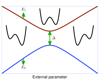
Figure 1: (Color online) Schematic diagram showing how two energy levels change with the external parameter for superconducting qubits. Here $E_{0}$ and $E_{1}$ are the eigenvalues of the ground and excited states, respectively. These vary with external parameters. For charge and flux qubits, the external parameters are the electric voltage and magnetic flux, respectively. At the degenerate (or optimal) point, where the external parameter takes a particular value, the energy splitting reaches a minimum, $\Delta=\hbar\omega_{x}$, where the double potential well is symmetric. In this case, there is only a SQ-field transverse coupling. However, when the external parameter deviates from this point, the double potential well is asymmetric, and there are both transverse and longitudinal couplings between the SQs and the applied electromagnetic field.

II Multi-photon process induced by a longitudinal coupling

II.1 Theoretical model

As schematically shown in Fig. 1, the shape of the potential energy for some kinds of SQs (e.g., charge and flux qubits) can be adjusted (from symmetric to asymmetric and vice versa) by an external parameter, and thus the two energy levels of SQs can also be controlled. For charge and flux qubits, the external parameters are the voltage and the magnetic flux, respectively. However the potential energy of the phase qubits is always broken, no matter how the external field is changed. The generic Hamiltonians for different types of SQs can be written as

$$H_{q}=\frac{\hbar}{2}\omega_{z}\sigma_{z}+\frac{\hbar}{2}\omega_{x}\sigma_{x}.$$ (1)

As in experiments, we assume that both parameters $\omega_{z}$ and $\omega_{x}$ can be controlled by external parameters. The parameter $\omega_{z}=0$ corresponds to the optimal point and well-defined inversion symmetry of the potential energy of the SQs. However, both nonzero parameters $\omega_{z}$ and $\omega_{x}$ correspond to a broken inversion symmetry of the potential energy of the SQs. Below, we first provide a general discussion based on the qubit Hamiltonian in Eq. (1), and then we will specify our discussions to different types of SQs. The discussion of their experimental feasibilities will be presented after the general theory.

Let us now assume that a SQ is coupled to a single-mode cavity field and is driven by a classical field, where the Hamiltonian of the driven superconducting qubits is

$$H=H_{q}+\hbar\omega a^{\dagger}a+\hbar g\sigma_{z}(a+a^{\dagger})+\hbar\Omega_{d}\sigma_{z}\cos(\omega_{d}t+\phi_{d}).$$ (2)

Here, $a^{\dagger}(a)$ is the creation (annihilation) operator of a single-mode cavity field with frequency $\omega$. The parameter $\Omega_{d}$ is the coupling constant between the SQ and the classical driving field with frequency $\omega_{d}$. The parameter $g$ is the coupling constant between the SQ and the single-mode cavity field. The parameter $\phi_{d}$ is the initial phase of the classical driving field.

Equation (2) shows that there are transverse and longitudinal couplings between the SQs and the electromagnetic field. This can become clearer if we rewrite the Hamiltonian in Eq. (2) in the qubit basis, that is,

$$H =\frac{\hbar}{2}\omega_{q}\widetilde{\sigma}_{z}+\hbar\omega a^{\dagger}a+\hbar g_{z}\widetilde{\sigma}_{z}(a+a^{\dagger})+\hbar g_{x}\widetilde{\sigma}_{x}(a+a^{\dagger})$$

$$+\hbar\Omega_{dz}\widetilde{\sigma}_{z}\cos(\omega_{d}t+\phi_{d})+\hbar\Omega_{dx}\widetilde{\sigma}_{x}\cos(\omega_{d}t+\phi_{d}),$$ (3)

with four parameters $g_{z}=g\cos\theta$, $g_{x}=-g\sin\theta$, $\Omega_{dz}=\Omega_{d}\cos\theta$, and $\Omega_{dx}=-\Omega_{d}\sin\theta$. Here, the parameter $\theta$ is given by $\theta=\arctan(\omega_{x}/\omega_{x})$, and the qubit eigenfrequency is $\omega_{q}=\sqrt{\omega_{x}^{2}+\omega_{z}^{2}}$.

The Hamiltonian in Eq. (3) shows that the qubit has both transverse and longitudinal couplings to the cavity (driving) fields with transverse $g_{x}$ ($\Omega_{x}$) and longitudinal $g_{z}$ ($\Omega_{z}$) coupling strengths. When both $\omega_{z}=0$ and $\Omega_{d}=0$, Eq. (3) is reduced to

$$\widetilde{H}=\frac{\hbar}{2}\omega_{q}\widetilde{\sigma}_{z}+\hbar g\widetilde{\sigma}_{x}(a+a^{\dagger})$$ (4)

which has only the transverse coupling between the SQ and the single-mode field. If we further make the rotating-wave approximation, then Eq. (4) can be reduced to the Jaynes-Cumming model, which has been extensively studied in quantum optics scullybook . That is, there is only a single-photon transition process when the qubit is at the optimal point. However, the transverse and the longitudinal couplings between the SQ and the single-mode field coexist, when the inversion symmetry of the potential energy is broken and $\omega_{z}$ is nonzero for the SQs. As shown below, this coexistence can induce multi-photon transitions between energy levels of SQs and make it easy to prepare arbitrary nonclassical states of the cavity field.

Below, we assume that both $\omega_{z}$ and $\omega_{x}$ are nonzero. We also assume that the SQ and the quantized field satisfy the large-detuning condition, that is,

$$\omega_{q}=\sqrt{\omega_{x}^{2}+\omega_{z}^{2}}\,\gg\omega.$$ (5)

In this case, the SQ and the quantized field are nearly decoupled from each other when the classical driving field is applied to the SQs.

II.2 Multi-photon processes and sideband excitations

Let us now study how multi-photon processes can be induced via a longitudinal coupling by first applying a displacement operator

$$D\left(\eta\frac{\sigma_{z}}{2}\right)=\exp\left[\eta\frac{\sigma_{z}}{2}(a^{\dagger}-a)\right],$$ (6)

to Eq. (2) with

$$\eta=2g/\omega.$$ (7)

Thus $\eta$ is the normalized qubit-cavity coupling. It is also known as the Lamb-Dicke parameter. Hereafter, we denote the picture after the transformation $D\left(\eta\sigma_{z}/2\right)$ as the displacement picture. In this case, we have an effective Hamiltonian

$$H_{\mathrm{eff}}\ =\ DHD^{\dagger}\ =\ \frac{\hbar}{2}\omega_{z}\sigma_{z}+\hbar\omega a^{\dagger}a+\hbar\Omega_{d}\sigma_{z}\cos(\omega_{d}t+\phi_{d})$$

$$+\frac{\hbar}{2}\omega_{x}\left\{\sigma_{+}\exp\left[\eta\left(a^{\dagger}-a\right)\right]+\mathrm{h.c.}\right\}.$$ (8)

From Eq. (8) with $\Omega_{d}=0$, we find that if $n\omega=\omega_{z}$, then the multiphoton processes, induced by the longitudinal coupling, can occur between two energy levels formed by the eigenstates of the operators $\sigma_{z}$. However, such process is not well controlled. Moreover, $\omega_{z}$ is usually not perfectly equal to $n\omega$, for arbitrarily chosen $n$. These problems can be solved by applying a classical driving field, in this case $\Omega_{d}\neq 0$.

To understand how the classical field can assist the cavity field to realize multi-photon processes in a controllable way, let us now apply another time-dependent unitary transformation

$$U_{d}\left(t\right)=\exp\left[\frac{i}{\hbar}H_{d}\left(t\right)\right]$$ (9)

to Eq. (8) with the Hamiltonian $H_{d}$ defined as

$$H_{d}\left(t\right)=\frac{\hbar\Omega_{d}\sigma_{z}}{\omega_{d}}\sin(\omega_{d}t+\phi_{d}),$$ (10)

and then we can obtain another effective Hamiltonian

$$H_{\mathrm{eff}}^{\left(d\right)} =U_{d}H_{\mathrm{eff}}U_{d}^{\dagger}-iU_{d}\frac{\partial U_{d}^{\dagger}}{\partial t}=\frac{\hbar}{2}\omega_{z}\sigma_{z}+\hbar\omega a^{\dagger}a$$

$$+\frac{\hbar\omega_{x}}{2}\sum_{N=-\infty}^{\infty}\left\{J_{N}\sigma_{+}B_{N}(t)+\text{H.c.}\right\},$$ (11)

where the time-dependent expression $B_{N}\left(t\right)$ is given as

$$B_{N}\left(t\right)=\exp\left[\eta\left(a^{\dagger}-a\right)+iN(\omega_{d}t+\phi_{d})\right];$$ (12)

$J_{N}\equiv J_{N}\left({x_{d}}\right)$ is the $N$th Bessel function of the first kind, with $x_{d}=2\Omega_{d}/\omega_{d}$ and $J_{N}({x_{d}})=(-1)^{N}J_{-N}({x_{d}})$, and $\eta$ is similar to the Lamb-Dicke parameter in trapped ions  trappedions ; wei . Via the unitary

$$V_{0}\left(t\right)=\exp\left[\frac{i}{\hbar}H_{0}t\right],$$ (13)

with

$$H_{0}=\frac{\hbar}{2}\omega_{z}\sigma_{z}+\hbar\omega a^{\dagger}a,$$ (14)

we can further expand the Hamiltonian in Eq. (11), in the interaction picture, into

$$H_{\mathrm{int}}=\frac{\hbar}{2}\omega_{x}\sum_{N,m,n}\left\{J_{N}^{mn}(t)\sigma_{+}a^{\dagger m}a^{n}+\mathrm{h.c.}\right\},$$ (15)

with

$$J_{N}^{mn}(t) =\frac{(-1)^{n}J_{N}}{m!n!}\eta^{m+n}\exp\left[-\frac{1}{2}\left(\eta\right)^{2}\right]$$ (16)

$$\times\exp\left[iN(\omega_{d}t+\phi_{d})+i\left(m-n\right)\omega t+i\omega_{z}t\right].$$

Equation (15) clearly shows that the couplings between the SQs and the quantized cavity fields can be controlled via a classical field when they are in the large-detuning regime. Comparing the Hamiltonian in Eq. (15) with that for the trapped ions trappedions ; wei , we find that the Hamiltonian in Eq. (15) is very similar to that of the two-level ion, confined in a coaxial-resonator-driven rf trap which provides a harmonic potential along the axes of the trap. Therefore, in analogy to the case of trapped ions, there are two controllable multi-photon processes (called red and blue sideband excitations, respectively) and one carrier process:

(i) when $n>m$, with $n-m=k$, and the transition satisfies the resonant condition $N\omega_{d}=\omega_{z}-k\omega$, with $N,\,k=1,\,2,\,3,\cdots$, the driving frequency $N\omega_{d}$ is red-detuned from the qubit frequency $\omega_{z}$. Thus, we call this multi-photon process the red process.

(ii) when $n<m$, with $m-n=k$, and the transition satisfies the resonant condition $N\omega_{d}=\omega_{z}+k\omega$, with $N,\,k=1,\,2,\,3,\cdots$, the driving frequency $N\omega_{d}$ is blue-detuned from the qubit frequency $\omega_{z}$. Then we call this process the blue process.

(iii) when $n=m$ and $\omega_{z}=N\omega_{d}$ ($N=1,\,2,\,\cdots$), the driving field with $N$ photons can resonantly excite the qubit. We call this transition the carrier process.

However, there are also differences between the Hamiltonian for trapped ions trappedions ; wei and that in Eq. (15). These differences are:

(i) For a given frequency $\omega_{d}$ of the driving field, there is only one multi-photon-transition process in the system of trapped ions to satisfy the resonant condition, but the SQs can possess several different multiphoton processes, resulting from the longitudinal coupling between the classical field and the SQ. For instance, with the given frequencies $\omega_{d}$ and $\omega$, and for the couplings with the $N$th and $N^{\prime}$th Bessel functions, two transitions with the red sideband resonant conditions: $N\omega_{d}=\omega_{z}-k\omega$ and $N^{\prime}\omega_{d}=\omega_{z}-k^{\prime}\omega$, might be satisfied. Once the condition $(N-N^{\prime})/(k^{\prime}-k)=\omega/\omega_{d}$ is satisfied, then these two resonant transitions can simultaneously occur. Similarly, for the case of blue-sideband excitations, the condition that two resonant transitions simultaneously occur for the $k$ and $k^{\prime}$ photon processes is $(N-N^{\prime})/(k-k^{\prime})=\omega/\omega_{d}$. We can represent the transition type in the sign of $k$ and $k^{\prime}.$ Thus if we want some terms with $N^{\prime}$ unresonant, all we need to do is to let $(N-N^{\prime})/(k-k^{\prime})\neq\omega/\omega_{d},$ i.e., $\omega_{z}\neq\omega\left(N^{\prime}k-Nk^{\prime}\right)/\left(N^{\prime}-N\right).$ One sufficient condition is that $\omega_{z}\neq\omega n/\left(N^{\prime}-N\right)$ ($n=0,\pm 1,\pm 2,$ $\cdots$).

(ii) The Lamb-Dicke parameter $\eta$ for the trapped ions is determined by the frequency of the vibration phonon, mass of the ion, and the wave vector of the driving field. However the Lamb-Dicke parameter $\eta$ here is determined by the frequency $\omega$ of the single-mode quantized field and the coupling constant $g$ between the single-mode field and the SQ.

(iii) For multi-photon processes, the coupling between trapped ions and the phonon is always on. However, such processes can in principle be switched off at the zeros of the Bessel functions of the first kind.

(iv) The term in Eq. (15) with $N=0$ means that the driving field has no help for the excitation of the SQ. Thus this term is neglected in the following discussions. However, the driving field can always be used to excite the trapped ions when certain resonant condition is satisfied.

(v) For trapped ions, the ratio between the transition frequency of the qubit and the frequency of the vibration quanta is often about $10^{9}$. Thus the upper bound for the photon number $k$ in the multiphotn process is about $k=10^{9}$. However, in the SQ circuit, the frequency of the SQ can be several tens of GHz, and the quantized cavity field can be in the regime of GHz. Thus the photon number $k$ is not extremely large. For example, if $\omega_{z}=20$ GHz and $\omega=2$ GHz, then the upper bound for $k$ is $10$.

To compare similarities and differences, Table  1 lists the main parameters of the Hamiltonian for trapped ions and those of the SQ in Eq. (11). We should note that the Lamb-Dicke parameter $\eta$ can become very large in circuit QED systems in the ultrastrong Niemczyk ; Forn ; Ultrastrong3 and deep-strong Casanova ; Braak ; Solano ; Liberato coupling regime. Our discussion below is in the ultrastrong coupling, but can be straightforwardly extended to the deep-strong coupling regime.

Table 1: Comparison of some parameters between the Hamiltonian in Eq. (15) and that of the trapped ions (e.g., in Ref. wei ). Here LD refers to the Lamb-Dicke parameter.

Parameters	Superconducting qubits (orders of magnitude)	Trapped ions (orders of magnitude)
LD parameters	$2g/\omega\sim(0.2-1.8)$	$\eta\sim(0.2-0.9)$
Carrier Rabi frequencies	Renormalized $J_{N}\>\omega_{x}/2$	Renormalized $\Omega$
Driving field frequencies	$\omega_{d}\,(N=1,\,\cdots)$	$\omega_{L}$

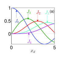
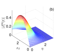
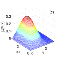
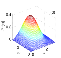
Figure 2: (Color online) Bessel functions $J_{N}(x_{d})$ of the first kind, with $N=0,\;1,\;2,\;3$, are plotted as functions of the ratio $x_{d}$ in (a). $\left|J_{1}^{00}(t)\right|$, $\left|J_{1}^{01}(t)\right|$, and $\left|J_{1}^{11}(t)\right|$ have been plotted in (b), (c), and (d) as functions of $\eta$ and $x_{d}$, respectively. Recall that $x_{d}=2\Omega_{d}/\omega_{d}$ is the ratio between the driving field-SQ Rabi frequency $\Omega_{d}$ and the frequency $\omega_{d}$ of the driving field.

II.3 Bessel functions and coupling strengths

In the process of generating nonclassical photon states, the coupling strength $J_{N}^{mn}(t)$ plays an important role. In our study here, the Bessel functions of the first kind are crucial factors in the coupling strengths. The possible values of the Bessel functions depend on the ratio $x_{d}$ between the driving field-SQ Rabi frequency $\Omega_{d}$ and the frequency $\omega_{d}$ of the driving field. For several recent experiments with superconducting quantum circuits, the coupling constant $\Omega_{d}$ is usually in the range from several tens of MHz to several hundreds of MHz, e.g., $10\,\mathrm{MHz}<\Omega_{d}<500$ MHz. The frequency $\omega_{d}$ of the driving field is in the range of GHz, e.g., $1\,\mathrm{GHz}\leq\omega_{d}\leq 20$ GHz. Thus the ratio $x_{d}$ is in the range

$$10^{-9}\leq x_{d}\leq 1.$$ (17)

For completeness and to allow a comparison between them, several Bessel functions are plotted as a function of the parameter $x_{d}=2\Omega_{d}/\omega_{d}$ in Fig. 2(a), which clearly shows $J_{0}(x_{d})>J_{1}(x_{d})>J_{2}(x_{d})>\cdots>J_{N}(x_{d})$ in the range of $10^{-9}\leq x_{d}\leq 1$. Thus if the classical driving field is chosen such that the ratio $x_{d}$ is less than $0.5$, then we only need to consider the terms in the Hamiltonian in Eq. (15) with the Bessel functions $J_{0}(x_{d})$ and $|J_{1}(x_{d})|=|J_{-1}(x_{d})|$, and other terms are negligibly small. As discussed above, it should be noted that the frequency $\omega_{d}$ of the driving field has no effect on the coupling between the SQ and the quantized field in terms of the Bessel function $J_{0}(x_{d})$. Thus the driving-field-assisted transitions between the SQ and the quantized field are determined by the terms with the Bessel functions $J_{\pm 1}(x_{d})$, when other high-order Bessel functions are neglected. Figure 2(a) also shows that the terms with the Bessel function $J_{\pm 2}(x_{d})$ are also not negligible when $x_{d}$ becomes larger, e.g., $0.5\leq x_{d}<1$. Thus in the regime $0\leq x_{d}<1$, the terms with high-order Bessel functions (e.g., the ones with $N\geq 3$) can be neglected.

As an example, Figs. 2(b, c, d) illustrate how $\left|J_{1}^{mn}(t)\right|$ are affected by $m$, $n$, $x_{d}$, and $\eta$. Since the maximal point occurs at $\eta=\sqrt{m+n}$, if other variables are fixed, thus we can find an obvious shift of the maximal point along the $\eta$-axis with increasing $m+n$. We can also find that $\left|J_{N}^{mn}(t)\right|$ have similar results as those of $\left|J_{1}^{mn}(t)\right|$ versus $m$, $n$, $x_{d}$, and $\eta$. By tuning $x_{d}$ and $\eta$, we can change the Rabi frequencies, and thus optimize the generation time.

III Generating non-classical photon states using superconducting quantum circuits

In this section, we discuss how to generate non-classical photon states via transverse and longitudinal couplings between SQs and the single-mode cavity field, with the assistance of a classical driving field.

III.1 Interaction Hamiltonian and time-evolution operators

Let us now analyze the interaction Hamiltonian and time evolutions for the three different processes based on the Hamiltonian in Eq. (15). We have three different interaction Hamiltonians. In the interaction picture with the resonant conditions of different photon processes, by assuming $n=m+k$ for the red-sideband excitation, $m=n+k$ for the blue-sideband excitation, and $m=n$ for the carrier process. We now discuss the general case for coupling constants with any number of Bessel functions. For a red process with the $N$th Bessel functions, we derive the Hamiltonian

$$H_{r}=J_{N,r}^{\left(k\right)}\sum_{m}\frac{(-1)^{m}\eta^{2m}\sigma_{+}a^{\dagger m}a^{m+k}}{m!(m+k)!}+\mathrm{h.c.},$$ (18)

with the resonant condition

$$N\omega_{d}=\omega_{z}-k\omega.$$

For a blue process with the $N$th Bessel functions, we have the Hamiltonian

$$H_{b}=J_{N,b}^{\left(k\right)}\sum_{n}\frac{(-1)^{n}\eta^{2n}\sigma_{+}a^{\dagger(n+k)}a^{n}}{n!(n+k)!}+\mathrm{h.c.},$$ (19)

with the resonant condition

$$N\omega_{d}=\omega_{z}+k\omega.$$

The parameters $J_{N,r}^{k}$ and $J_{N,b}^{k}$ for the red process in Eq. (18) and the blue one in Eq. (19) are given by

$$J_{N,r}^{\left(k\right)} =(-1)^{k}\frac{\omega_{x}}{2}J_{N}\exp\left[-\frac{1}{2}\left(\frac{2g}{\omega}\right)^{2}+iN\phi_{d}^{\left(\beta\right)}\right]\eta^{k},$$ (20)

$$J_{N,b}^{\left(k\right)} =\frac{\omega_{x}}{2}J_{N}\exp\left[-\frac{1}{2}\left(\frac{2g}{\omega}\right)^{2}+iN\phi_{d}^{\left(\beta\right)}\right]\eta^{k},$$ (21)

where the subscript $\beta$ takes either $r$ or $b$, we use $\phi_{0}^{\left(\beta\right)}$ to characterize the initial phase of either the red or the blue process. For the carrier process with the $N$th Bessel functions, the interaction Hamiltonian is given by

$$H_{c}=J_{N,c}^{\left(0\right)}\sum_{n}\eta^{2n}\frac{(-1)^{n}\sigma_{+}a^{\dagger n}a^{n}}{n!n!}+\mathrm{h.c.},$$ (22)

with the resonant condition

$$N\omega_{d}=\omega_{z},$$

and the coupling constant

$$J_{N,c}^{\left(0\right)}=\frac{1}{2}\omega_{x}J_{N}\exp\left[-\frac{1}{2}\eta^{2}+iN\phi_{d}^{\left(c\right)}\right].$$ (23)

We also note that all non-resonant terms have been neglected when Eqs. (18-22) are derived. The dynamical evolutions of the systems corresponding to these three different processes can be described via time-evolution operators. For example, for the $k$th red, blue, and carrier sideband excitations, we respectively have the evolution operators

$$U_{N,r}^{\left(k\right)}\left(t\right)= \sum_{n=0}^{k-1}\left|n\right\rangle\left\langle n\right|\sigma_{00}+\sum_{n=0}^{\infty}\cos\left(\left|\Omega_{N,r}^{k,n}\right|t\right)\left|n\right\rangle\left\langle n\right|\sigma_{11}$$

$$+\sum_{n=0}^{\infty}e^{-i\phi_{N,r}^{k,n}-i\pi/2}\mathrm{sin}\left(\left|\Omega_{N,r}^{k,n}\right|t\right)\left|n+k\right\rangle\left\langle n\right|\sigma_{-}$$

$$+\sum_{n=0}^{\infty}e^{i\phi_{N,r}^{k,n}-i\pi/2}\mathrm{sin}\left(\left|\Omega_{N,r}^{k,n}\right|t\right)\left|n\right\rangle\left\langle n+k\right|\sigma_{+}$$

$$+\sum_{n=0}^{\infty}\cos\left(\left|\Omega_{N,r}^{k,n}\right|t\right)\left|n+k\right\rangle\left\langle n+k\right|\sigma_{00},$$ (24)

$$U_{N,b}^{\left(k\right)}\left(t\right)= \sum_{n=0}^{k-1}\left|n\right\rangle\left\langle n\right|\sigma_{11}+\sum_{n=0}^{\infty}\cos\left(\left|\Omega_{N,b}^{k,n}\right|t\right)\left|n\right\rangle\left\langle n\right|\sigma_{00}$$

$$+\sum_{n=0}^{\infty}e^{i\phi_{N,b}^{k,n}-i\pi/2}\mathrm{sin}\left(\left|\Omega_{N,b}^{k,n}\right|t\right)\left|n+k\right\rangle\left\langle n\right|\sigma_{+}$$

$$+\sum_{n=0}^{\infty}e^{-i\phi_{N,b}^{k,n}-i\pi/2}\mathrm{sin}\left(\left|\Omega_{N,b}^{k,n}\right|t\right)\left|n\right\rangle\left\langle n+k\right|\sigma_{-}$$

$$+\sum_{n=0}^{\infty}\cos\left(\left|\Omega_{N,b}^{k,n}\right|t\right)\left|n+k\right\rangle\left\langle n+k\right|\sigma_{11},$$ (25)

and

$$U_{N,c}^{\left(0\right)}\left(t\right)= \sum_{n=0}^{\infty}\cos\left(\left|\Omega_{N,c}^{0,n}\right|t\right)\left|n\right\rangle\left\langle n\right|\sigma_{11}$$

$$+\sum_{n=0}^{\infty}e^{-i\phi_{N,c}^{0,n}-i\pi/2}\mathrm{sin}\left(\left|\Omega_{N,c}^{0,n}\right|t\right)\left|n\right\rangle\left\langle n\right|\sigma_{-}$$

$$+\sum_{n=0}^{\infty}e^{i\phi_{N,c}^{0,n}-i\pi/2}\mathrm{sin}\left(\left|\Omega_{N,c}^{0,n}\right|t\right)\left|n\right\rangle\left\langle n\right|\sigma_{+}$$

$$+\sum_{n=0}^{\infty}\cos\left(\left|\Omega_{N,c}^{0,n}\right|t\right)\left|n\right\rangle\left\langle n\right|\sigma_{00},$$ (26)

where the complex Rabi frequency and its phase angle are respectively defined as

$$\Omega_{N,\beta}^{k,n} =J_{N,\beta}^{(k)}\sqrt{\frac{n!}{\left(n+k\right)!}}L_{n}^{\left(k\right)}\left(\eta^{2}\right),$$ (27)

$$\phi_{N,\beta}^{k,n} =\arg\left(\Omega_{N,\beta}^{k,n}\right),$$ (28)

with $\beta=r,b,c$ and $J_{N,\beta}^{(k)}$ are given in Eqs. (20), (21), and (23). Here $L_{n}^{\left(k\right)}\left(x\right)$ represents the generalized Laguere polynomials. Let us assume that the two eigentates $|g\rangle$ and $|e\rangle$ of the Pauli operator $\sigma_{z}$ satisfy $\sigma_{z}\left|g\right\rangle=-\left|g\right\rangle$, and $\sigma_{z}\left|e\right\rangle=\left|e\right\rangle$, then we define the following operators $\sigma_{ii}$ as $\sigma_{00}=\left|g\right\rangle\left\langle g\right|$, $\sigma_{11}=\left|e\right\rangle\left\langle e\right|$, $\sigma_{01}=\left|g\right\rangle\left\langle e\right|$, and $\sigma_{10}=\left|e\right\rangle\left\langle g\right|$.

III.2 Synthesizing nonclassical photon states

We find that the interaction Hamiltonians in Eqs. (18-22) in the displacement picture are very similar to those for trapped ions wei . Therefore, in principle the non-classical photon states can be generated by alternatively using the above three different controllable processes. We expect that the prepared target state is

$$\left|\psi_{n_{\max}}\right\rangle=\sum_{n=0}^{n_{\max}}C_{n}\left|n\right\rangle\otimes\left|q\right\rangle,$$ (29)

where $n_{\max}$ is a maximal photon number in the photon state of the target state. Here, $\left|n\right\rangle\otimes\left|q\right\rangle\equiv\left|n\right\rangle\left|q\right\rangle$ denotes that the cavity field is in the photon number state $|n\rangle$ and the qubit is in the state $|q\rangle$, which can be either the ground $|g\rangle$ or excited $|e\rangle$ state. The parameter $|C_{n}|^{2}$ is the probability of the state $\left|n\right\rangle\otimes\left|q\right\rangle$. The steps for producing the target state for both the case $q=g$ and $q=e$ are very similar. We thus take $q=g$ as an example to present the detailed steps. The target state then takes the form

$$\left|\psi_{n_{\max}}\right\rangle=\sum_{k=0}^{n_{\max}}C_{k}\left|k\right\rangle\otimes\left|g\right\rangle.$$ (30)

We point out that all the states here (e.g., the target state) are observed in the displacement picture, if we do not specify this.

We assume that the system is initially in the state $\left|0\right\rangle\left|g\right\rangle$. Then, by taking similar steps as in Ref. wei , we can generate an arbitrary state in which the states $|\psi_{n}\rangle$ in the $n$th step and $|\psi_{n-1}\rangle$ in the $(n-1)$th step have the following relation,

$$\left|\psi_{n}\right\rangle=U_{0}^{(n){\dagger}}\left(t_{n}\right)U_{N,\beta_{n}}^{(n)}\left(t_{n}\right)U_{0}^{(n)}\left(0\right)\left|\psi_{n-1}\right\rangle,$$ (31)

with

$$\left|\psi_{n}\right\rangle=\sum_{k=0}^{n}C_{kg}^{\left(n\right)}\left|k\right\rangle\left|g\right\rangle+C_{0e}^{\left(n\right)}\left|0\right\rangle\left|e\right\rangle.$$ (32)

Here if $n=n_{\max}$, $\ C_{0e}=0$, and $C_{kg}^{\left(n\right)}=C_{k}$, then $\left|\psi_{n}\right\rangle$ in Eq. (32) is reduced to $\left|\psi_{n_{\max}}\right\rangle$ in Eq. (30). Above, $t_{n}$ is the time duration of the control pulse for the $n$th step. The unitary transform $U_{0}^{(n)}\left(t\right)$ is defined as

$$U_{0}^{(n)}\left(t\right)=V_{0}\left(t\right)U_{d}^{\left(n\right)}\left(t\right).$$ (33)

Here $V_{0}\left(t\right)$ is given in Eq. (13). Also, $U_{d}^{\left(n\right)}\left(t\right)$ is actually $U_{d}\left(t\right)$ in Eq. (9), but with $\omega_{d}$ and $\phi_{d}$ replaced by $\omega_{d}^{\left(n\right)}$ and $\phi_{d}^{\left(n\right)}$, which denote respectively the frequency and phase of the driving field for the $n$th step. Moreover, $U_{N,\beta_{n}}^{(n)}\left(t_{n}\right)$ denotes a unitary transform of the $n$th step, and is taken from one of Eq. (24), Eq. (25), and Eq. (26) depending on which one is chosen as $\beta_{n}$ among the characters “$r$”, “$b$”, and “$c$”. In $U_{N,\beta_{n}}^{(n)}\left(t_{n}\right)$, the parameters $\omega_{d}$ and $\phi_{d}$ must also be replaced by $\omega_{d}^{\left(n\right)}$ and $\phi_{d}^{\left(n\right)}$, respectively.

The target of the $n$th step is to generate the state $\left|\psi_{n}\right\rangle$ from the state $\left|\psi_{n-1}\right\rangle$. We assume $\left|\psi_{n-1}\right\rangle$ is in the displacement picture, which is the state generated after the $(n-1)$th step. We first use $U_{0}^{(n)}\left(t_{n}\right)$ to transfer $\left|\psi_{n-1}\right\rangle$ from the displaced picture into the interaction picture. Then we choose one of the evolution operators in Eqs. (24)–(26) with a proper photon number to reach the target state in Eq. (31). Since the state $\left|\psi_{n}\right\rangle$ should also be represented in the displaced picture, after the state of the $n$th step via the evolution operators $U_{N,\beta_{n}}^{(n)}\left(t_{n}\right)$ and $U_{0}^{(n)}\left(0\right)$, we have to transfer it back to the displaced picture, which results in the appearance of $U_{0}^{(n){\dagger}}\left(t_{n}\right)$ in Eq. (31).

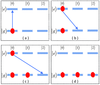
Figure 3: (Color online) Schematic diagram for state generation of the target state $\left|\psi_{n_{\max}}\right\rangle=\sum_{k=0}^{n_{\max}}C_{k}\left|k\right\rangle\otimes\left|g\right\rangle$, for example, $n_{\max}=2$. (a) Step 0, the system is initially in the state $\left|0\right\rangle\otimes\left|g\right\rangle$, and the arrow means that a carrier process is applied with the $0$-photon inside the cavity, denoted by the operator $U_{N,c}^{(0)}\left(t_{0}\right)$. (b) Step 1, after the step $0$, the system is in the state $C_{0g}^{\left(0\right)}\left|0\right\rangle\otimes\left|g\right\rangle+C_{0e}^{\left(0\right)}\left|0\right\rangle\otimes\left|e\right\rangle$, in which the parameters $C_{0e}^{\left(0\right)}$ and $C_{0g}^{\left(0\right)}$ are determined by the time duration $t_{0}$. The arrow means that a $1$-photon red process is applied with the time evolution operator $U_{N,r}^{\left(1\right)}\left(t_{1}\right)$ after the step $0$. (c) Step 2, after the step $1$, the system is in the state $C_{0g}^{\left(1\right)}\left|0\right\rangle\otimes\left|g\right\rangle+C_{1g}^{\left(1\right)}\left|1\right\rangle\otimes\left|g\right\rangle+C_{0e}^{\left(1\right)}\left|0\right\rangle\otimes\left|e\right\rangle$, in which the coefficients of the superposition are determined by the time duration $t_{0}$ and $t_{1}$. The arrow means that a $2$-photon red process $U_{N,r}^{\left(2\right)}\left(t_{2}\right)$ is applied to the system after the step $1$. (d) After the step $2$ (with well-chosen time durations $t_{0}$, $t_{1}$ and $t_{2}$), the system is in the state $C_{0}\left|0\right\rangle\otimes\left|g\right\rangle+C_{1}\left|1\right\rangle\otimes\left|g\right\rangle+C_{2}\left|2\right\rangle\otimes\left|g\right\rangle$, which is just the target state $\left|\psi_{2}\right\rangle$. Other superpositions can also be generated using similar steps.

The longitudinal coupling results in multi-photon processes. Thus the state preparation using the longitudinal coupling is in principle more convenient than that using a single-photon transition in the usual Jaynes-Cumming model liuepl . For example, the Fock state $|n\rangle$ can be generated with a carrier process and a longitudinal coupling field-induced $n$-photon process. However, it needs $2n$ steps ($n$ step carrier and $n$ step red-sideband processes) to produce a Fock state $|n\rangle$ if we use the Jaynes-Cumming model liuepl . The selection of $U_{N,\beta_{n}}^{\left(n\right)}\left(t_{n}\right)$ in Eq. (31) for each step is almost the same as that in Ref. wei . That is, the target state in Eq. (30) can be obtained either by virtue of one carrier process and $n_{\mathrm{max}}$ red-sideband excitations, or by virtue of one carrier process and $n_{\mathrm{max}}$ blue-sideband excitations.

The steps to generate the target state in Eq. (30) from the initial state $|0\rangle|g\rangle$ using carrier and red sideband excitations are schematically shown in Fig. 3 using a simple example. All steps for the required unitary transformations are described as follows. First, the initial state $\left|0\right\rangle\left|g\right\rangle$ is partially excited to $\left|0\right\rangle\left|e\right\rangle$ by a carrier process ($n=0$) with a time duration $t_{0}$ such that the probability $|C_{0g}^{(0)}|^{2}$ in $\left|0\right\rangle\left|g\right\rangle$ satisfies the condition $|C_{0g}^{(0)}|^{2}=|C_{0}|^{2}$, with $C_{0}$ given in Eq. (30). After the carrier process, the driving fields are sequentially applied to the qubit with $n_{\mathrm{max}}$ different frequency matching conditions, such that a single-photon, two-photon, until $n_{\mathrm{max}}$-photon red processes can occur. Thus the subscript $\beta_{n}$ in the unitary transform $U_{N,\beta_{n}}^{(n)}$ satisfies the conditions $\beta_{n}=c$ with $n=0$, and $\beta_{n}=r$ for $n\geq 1$. By choosing appropriate time durations and the phases of the driving fields in each step, which in principle can be obtained using Eq. (31), we can obtain the target state shown in Eq. (30). The detailed descriptions can be found in Appendix A.

IV The initial state and target state

Above, we assumed that the target state is generated from the initial state which is the vacuum state in the displacement picture defined by Eq. (6). However, in experiments, the initial state is usually the ground state, obtained by cooling the sample inside a dilution refrigerator. We now investigate the ground state of the effective Hamiltonian when there is no driving field. The Hamiltonian $H_{\mathrm{eff}}$ without driving field can be expressed as

$$H_{\mathrm{eff}}^{\prime}=\frac{\hbar}{2}\omega_{z}\sigma_{z}+\hbar\omega a^{\dagger}a+\frac{\hbar}{2}\omega_{x}\left\{\sigma_{+}\exp\left[\eta\left(a^{\dagger}-a\right)\right]+\mathrm{h.c.}\right\},$$ (34)

in the displacement picture. However, in the original picture, the corresponding Hamiltonian is

$$H^{\prime}=\frac{\hbar}{2}\omega_{z}\sigma_{z}+\frac{\hbar}{2}\omega_{x}\sigma_{x}+\hbar\omega a^{\dagger}a+\hbar g\sigma_{z}(a+a^{\dagger}),$$ (35)

which possesses the characteristics of broken-symmetry and strong coupling and is hence difficult to solve analytically. Due to the mathematical equivalence between Eq. (34) and Eq. (35), it is also difficult to solve Eq. (34) analytically. We thus resort to numerical calculations to obtain the ground state of $H_{\mathrm{eff}}^{\prime}$. We define the ground state of the Hamiltonian $H_{\mathrm{eff}}^{\prime}$ as $\left|\psi_{g}\right\rangle$, and the probability of the ground state $\left|\psi_{g}\right\rangle$ to be in the vacuum state $\left|0\right\rangle$ as $P_{g,0}$. The relation between $\left|\psi_{g}\right\rangle$ and $P_{g,0}$ can be written as

$$\left|\psi_{g}\right\rangle =\left[\xi_{0}\left|0\right\rangle+\sqrt{1-|\xi_{0}|^{2}}\left|\delta\psi_{g}\right\rangle\right]|g\rangle,$$ (36)

$$P_{g,0} =\left|\xi_{0}\right|^{2},$$ (37)

where $|\delta\psi_{g}\rangle$ denotes a superposition of photon number states except the vacuum state. In Fig. 4, as an example, by taking $\omega_{z}/2\pi=19.5$ GHz and $\omega=2$ GHz, we have plotted $P_{g,0}$ as a function of $\eta$ and $\omega_{x}$. We find that the probability $P_{g,0}\geq 0.99$, at least in the region $0<\eta<3.5$ and $0<\omega_{x}/\omega_{z}<0.2$. More specifically, the ground state of the Hamiltonian in Eq. (34) is closer to the vacuum state when the parameters $\eta$ and $\omega_{x}$ are smaller. Thus, our assumption that the initial state of the cavity field in the displacement picture is the vacuum state, can always be valid only if the related parameters, such as $\omega_{x}$ and $\eta$, are properly chosen.

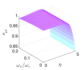
Figure 4: (Color online) Probability $P_{g,0}$ for the ground state to be the vacuum state in the displacement picture as a function of $\eta$ and $\omega_{x}/\omega_{z}$. Here we assume $\omega_{z}/2\pi=19.5\operatorname{GHz}$, and $\omega=2\operatorname{GHz}$. Recall that $\eta$ is the normalized coupling or the Lamb-Dicke parameter.

We have demonstrated how to generate an arbitrary superposition of different Fock sates from the vacuum state in the displacement picture. Thus, once the state is generated, we have to displace the generated state back to the original picture via the displacement operator $D^{\dagger}\left(\eta\sigma_{z}/2\right)$. For example, the initial state $|0\rangle|g\rangle$ in the displacement picture becomes

$$D^{{\dagger}}\left(\frac{\eta}{2}\sigma_{z}\right)|0\rangle|g\rangle=\left|\frac{\eta}{2},0\right\rangle\left|g\right\rangle,$$ (38)

in the original picture, where $\left|\alpha,n\right\rangle=$ $D\left(\alpha\right)\left|n\right\rangle$ denotes the displaced number state Oliveira1990 . Similarly, the target state $\left|\psi_{n_{\max}}\right\rangle$ in the displacement picture becomes

$$\left|\psi_{n_{\max}}^{D}\right\rangle=\sum_{n=0}^{n_{\max}}C_{n}\left|\frac{\eta}{2},n\right\rangle\left|g\right\rangle,$$ (39)

in the original picture. It is obvious that the initial state $\left|\eta/2,0\right\rangle$ of the cavity field in the original picture is a coherent state with the average photon number $\left(\eta/2\right)^{2}$, while the target state is the superposition of the displaced number states.

The statistical properties of a displaced number state with $D(\alpha)|n\rangle$ can be described by the probabilities of the photon number distribution as below

$$\left\langle l|\alpha,n\right\rangle=\left\{\begin{array}[c]{ll}\frac{\alpha^{l-n}\sqrt{n!/l!}}{\exp\left(\left|\alpha\right|^{2}/2\right)}L_{n}^{\left(l-n\right)}\left(\left|\alpha\right|^{2}\right),&\,l\geq n,\\ \\ \frac{\left(-\alpha^{\ast}\right)^{\left(n-l\right)}\sqrt{l!/n!}}{\exp\left(\left|\alpha\right|^{2}/2\right)}L_{l}^{\left(n-l\right)}\left(\left|\alpha\right|^{2}\right),&\,l<n.\end{array}\right.$$ (40)

Thus the displaced target state in Eq. (39) can be written as

$$\left|\psi_{n_{\max}}^{D}\right\rangle =\sum_{n=0}^{n_{\max}}C_{n}\sum_{l=0}^{\infty}\left|l\right\rangle\left\langle l\right.\left|\frac{\eta}{2},n\right\rangle\left|g\right\rangle$$

$$=\sum_{l=0}^{\infty}C_{l}^{D}\left|l\right\rangle\left|g\right\rangle,$$ (41)

where $C_{l}^{D}=\sum_{n=0}^{n_{\max}}C_{n}\left\langle l|\eta/2,n\right\rangle$. The probability of the target sate $\left|\psi_{n_{\max}}^{D}\right\rangle$ to be in the photon number $\left|l\right\rangle$ in the original picture can be given as

$$P_{l}^{D}=\left|C_{l}^{D}\right|^{2}=\sum_{n=0}^{n_{\max}}\sum_{m=0}^{n_{\max}}C_{n}C_{m}^{\ast}\Big{\langle}l\left|\frac{\eta}{2},n\right\rangle\left\langle\frac{\eta}{2},m\right|l\Big{\rangle}.$$ (42)

In Fig. 5, as an example, the distribution probabilities $P_{l}^{D}$ are plotted for different photon states, that is, $\left|\psi_{n_{\max}}^{D}\right\rangle$ is taken as $\left|\eta/2,0\right\rangle\left|g\right\rangle,\left|\eta/2,2\right\rangle\left|g\right\rangle,$ or $\left(\left|\eta/2,0\right\rangle+\left|\eta/2,2\right\rangle\right)\left|g\right\rangle/\sqrt{2}$, which is $|0\rangle$, $|2\rangle$ and $(|0\rangle+|2\rangle)/\sqrt{2}$, respectively, in the displacement picture. Figure 5 shows that the photon number states in the displacement picture are redistributed after these states are sent back to the original picture. Even though the state in Fig. 5(c) is the linear sum of the states in Fig. 5(a) and Fig. 5(b), the photon number distributions are not linearly additive. Because the interference between different displaced number states, which corresponds to the terms of $m\neq n$ in Eq. (42), can also give rise to the variation of the photon number distribution. It is clear that a number state in the displaced picture can become a superposition of number states in the original picture, which might offer a convenient way to prepare nonclassical photon states.

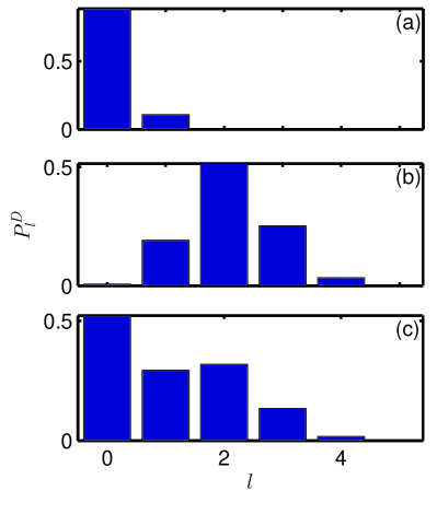
Figure 5: Photon number distributions of (a) $\left|\eta/2,0\right\rangle$, (b) $\left|\eta/2,2\right\rangle$, and (c) $\left(\left|\eta/2,0\right\rangle+\left|\eta/2,2\right\rangle\right)/\sqrt{2}$. Here $l$ refers to the photon number and $P^{D}_{l}$ refers to the probability on $\left|l\right\rangle$. We have taken the Lamb-Dicke parameter $\eta=2g/\Omega=0.7.$

V Numerical analysis

We have presented a detailed analysis on how to prepare nonclassical photon states using the longitudinal-coupling-induced multi-photon processes in an ideal case. In this ideal case, with the perfect pulse-duration and frequency-matching conditions, we can prepare the perfect target state. However, in practical cases, the system cannot avoid environmental effects. Moreover, the imperfection of the parameters chosen also affects the fidelity of the target state. For example, different $N$ describe different Bessel functions for effective coupling strengths between the cavity field, the two-level system, and the classical driving field. Then the optimization for the target state will also be different. For concreteness, as an example, let us study the effects of both the environment and imperfect parameters on the target state

$$\left|\psi_{02}\right\rangle=\frac{1}{\sqrt{2}}\left(\left|0\right\rangle+\left|2\right\rangle\right)\left|g\right\rangle,$$ (43)

in the displacement picture, whose density matrix operator can be given as

$$\rho^{I}=\left|\psi_{02}\right\rangle\left\langle\psi_{02}\right|.$$ (44)

We also assume that the terms with the Bessel function for $N=-1$ are chosen for the state preparation. But other terms with the Bessel function order $N^{\prime}\neq N$ are also involved. Thus we have to choose $\omega_{z}\neq\omega n/\left(N^{\prime}-N\right)$ to minimize the effect of these terms. Among all the terms with the Bessel function order $N^{\prime}$, the dominant ones are those with $N^{\prime}=0,1,\pm 2$. That is, the chosen $\omega_{z}$ has to satisfy the condition $\omega_{z}\neq$ $n\omega,\,n\omega/2$, and $n\omega/3$.

To study the environmental effect on the state preparation, we assume that the dynamical evolution of the system satisfies the following master equation

$$\dot{\rho}=-i\left[H,\rho\right]+\mathcal{L}_{q}\left[\rho\right]+\mathcal{L}_{c}\left[\rho\right],$$ (45)

when the environmental effect is taken into account, where the Hamiltonian $H$ is given by Eq. (2) and

$$\mathcal{L}_{q}\left[\rho\right] =\frac{1}{2}\sum_{1\geq j\geq i\geq 0}\gamma_{ij}\left(2\tilde{\sigma}_{ij}\rho\tilde{\sigma}_{ji}-\tilde{\sigma}_{jj}\rho-\rho\tilde{\sigma}_{jj}\right),$$ (46)

$$\mathcal{L}_{c}\left[\rho\right] =\frac{\kappa}{2}\left(2a\rho a^{{\dagger}}-a^{{\dagger}}a\rho-\rho a^{{\dagger}}a\right),$$ (47)

describe the dissipation of the qubit and the cavity field, respectively. Here $\rho$ is the reduced density matrix of the qubit and the cavity field. And $\sigma_{ij}=|i\rangle\langle j|$, where we define $|0\rangle\equiv|g\rangle$, and $|1\rangle\equiv|e\rangle$. The operators $\tilde{\sigma}_{ij}$ are given by

$$\tilde{\sigma}_{ij}=R_{y}\left(\theta\right)\sigma_{ij}R_{y}^{\dagger}\left(\theta\right),$$

with $R_{y}\left(\theta\right)=\exp\left(-i\theta\sigma_{y}/2\right)$ and $\theta=\arctan\left(\omega_{x}/\omega_{z}\right)$. This is because we have used the eigenstates of $\sigma_{z}$ as a basis (persistent current basis) to represent the Hamiltonian of the qubit. Note that $\gamma_{10}$ is the the relaxation rate, while $\gamma_{11}$ and $\gamma_{00}$ are the dephasing rates. The parameter $\kappa$ is the decay rate of the cavity field. In the following calculations, we assume $\gamma_{00}=0$.

We first neglect the environmental effects and just study how the unwanted terms with the Bessel function for $N^{\prime}\neq-1$ affects the fidelity for different parameters $x_{d}=2\Omega_{d}/\omega_{d}$ and $\eta=2g/\omega$ of the driving field and the cavity field when the target state in Eq. (43) is prepared. We define the density matrix

$$\rho^{D}=\left|\psi_{02}^{D}\right\rangle\left\langle\psi_{02}^{D}\right|=D^{{\dagger}\!\!}\left(\eta/2\right)\rho^{I}D^{\!\!}\left(\eta/2\right)$$ (48)

which is the ideal target state in the original picture. The actual target state generated in the original picture is denoted by the density operator $\rho^{A}$ when the effect of the unwanted terms is taken into account. The Fidelity for the target state is then given by

$$F=\operatorname{Tr}\left\{\rho^{A}\rho^{D}\right\}.$$ (49)

Let us now take the parameters $\omega/2\pi=2$ GHz and $\omega_{z}/2\pi=19.5$ GHz as an example to show how the parameters affect the fidelity. The highly symmetry-broken condition is satisfied by taking, e.g., $\omega_{x}/2\pi=1.6$ GHz. We have listed the fidelities for different $\eta$ and $x_{d}$ in Table 2, from which we can find that larger values of $\eta$ and $x_{d}$ are more likely to induce a higher fidelity. Because in the range considered for $\eta$ and $x_{d}$, a larger $x_{d}$ can enhance the desired term through making $J_{-1}\left(x_{d}\right)$ larger [see Fig. 2(a)] while $\eta$ achieves the same goal by enhancing the Rabi frequency for $\left|0\right\rangle\left|e\right\rangle\longleftrightarrow$ $\left|2\right\rangle\left|g\right\rangle$ (see Fig. 7 in Appendix A).

In Table 2, the largest fidelity is $F_{m}=0.886$ which occurs at the optimal parameters $\eta=\eta_{m}=1.11$, and $x_{d}=x_{d}^{m}=$ $1.305$, where we have also obtained the total time $T_{m}=1.82$ ns for generating the target state. From the above numerical calculations, we show that the fidelity of the prepared target state is significantly affected by the parameters of the qubit, cavity field, and driving field. Note that the fidelities in Table 2 may not be satisfactory for practical applications in quantum information processing, which may require fidelities approaching 100%. However, the fidelity can be further optimized by carefully choosing suitable experimental parameters. For instance, $\eta=1.5$ and $x_{d}=1.305$ would produce a more desirable fidelity of 0.9143, and it is still possible to obtain much higher fidelities when related parameters are further optimized. We should also mention that the effect of the unwanted terms can be totally avoided if for each generation step, the control pulses for the driving frequency $\omega_{d}$, driving strength $\Omega_{d}$, driving phase $\phi_{d}$, and the pulse duration $t$ are all perfectly designed to compensate the effect of the unwanted terms.

Table 2: The fidelities of the target state are listed for different values of the parameters $x_{d}=2\Omega_{d}/\omega_{d}$ and $\eta=2g/\omega$. Here we have chosen $\omega_{z}/2\pi=19.5\operatorname{GHz}$, $\omega_{x}=1.6\operatorname{GHz}$, and $\omega=2\operatorname{GHz}$.

		Lamb-Dicke parameter $\eta=2g/\omega$
		$0.330$	$0.590$	$0.850$	$1.110$	$1.370$
	$0.265$	$0.240$	$0.219$	$0.237$	$0.347$	$0.332$
	$0.525$	$0.281$	$0.282$	$0.621$	$0.719$	$0.734$
$x_{d}=2\Omega_{d}/\omega$	$0.785$	$0.445$	$0.416$	$0.722$	$0.827$	$0.841$
	$1.045$	$0.369$	$0.519$	$0.780$	$0.857$	$0.877$
	$1.305$	$0.335$	$0.530$	$0.791$	$0.886$	$0.879$

Now we study the environmental effect on the fidelity of the prepared state by taking experimentally achievable parameters, e.g., $\gamma_{10}/2\pi=\kappa/2\pi=1$ MHz and $\gamma_{11}=2$ MHz. We also choose $\eta=\eta_{m}$ and $x_{d}=x_{d}^{m}$, and other parameters (i.e., $\omega_{x}$, $\omega_{z}$, and $\omega$) are kept the same as in Table 2. Now the fidelity we obtain via numerical calculations is $F_{m}^{\prime}=0.8775$.

The Wigner function represents the full information of the states of the cavity field and can be measured via quantum state tomography Leibfried1996 . The Wigner function of the cavity field has recently been measured in circuit QED systems Eichler2011 ; Shalibo2013 . To obtain the state of the cavity field, let us now trace out the qubit part of the density operator for the qubit-cavity composite system using the formula

$$\rho_{c}^{p}=\operatorname{Tr}_{q}\rho^{p}=\left\langle g\right|\rho^{p}\left|g\right\rangle+\left\langle e\right|\rho^{p}\left|e\right\rangle,$$ (50)

where $p$ refers to either $D$, $I$, or $A$. Here, $\rho^{I}$ is the ideal target state in the displacement picture, $\rho^{D}$ is the the ideal target state in the original picture, and $\rho^{A}$ is the actual target state in the original picture. Therefore, $\rho_{c}^{p}$ is the cavity part of the qubit-cavity-composite state $\rho^{p}$. It should be emphasized here that the actual state $\rho^{A}$ denotes the generated target state in the original picture with the same parameters as in the ideal case, but including the effects of both the environment and unwanted terms. By definition, given an arbitrary density operator $\rho,$ the Wigner function $\mathcal{W}\left(\beta,\beta^{\ast}\right)$ and the Wigner characteristic function $C^{W}\left(\lambda,\lambda^{\ast}\right)$ have the following relations Agarwal1991 ; Louisell1973 ; QuantumNoise ,

$$C^{W}\left(\lambda,\lambda^{\ast}\right) =\operatorname{Tr}\left\{\rho\exp\left(\lambda a^{{\dagger}}-\lambda^{\ast}a\right)\right\},$$ (51)

$$\mathcal{W}\left(\beta,\beta^{\ast}\right) =\int\frac{\text{{d}}^{2}\lambda}{\pi^{2}}\;C^{W}\left(\lambda,\lambda^{\ast}\right)\exp\left(-\lambda\beta^{\ast}+\lambda^{\ast}\beta\right).$$ (52)

Moreover, if $\rho$ is expanded in the Fock state space, i.e,

$$\rho=\sum_{mn}\rho_{mn}\left|m\right\rangle\left\langle n\right|,$$ (53)

then we have the Wigner function of $\rho$ given by

$$\mathcal{W}\left(\beta,\beta^{\ast}\right)=\sum_{mn}\rho_{mn}\mathcal{W}_{mn}\left(\beta,\beta^{\ast}\right),$$ (54)

where

$$\mathcal{W}_{mn}\left(\beta,\beta^{\ast}\right)=\left\{\begin{array}[c]{ll}\begin{array}[c]{l}\frac{2^{n-m+1}}{\pi}\left(-1\right)^{m}\sqrt{\frac{m!}{n!}}\;\beta^{n-m}\\ \times e^{-2\left|\beta\right|^{2}}L_{m}^{\left(n-m\right)}\left(4\left|\beta\right|^{2}\right),\end{array}&m<n,\\ \\ \begin{array}[c]{l}\frac{2^{m-n+1}}{\pi}\left(-1\right)^{n}\sqrt{\frac{n!}{m!}}\;\beta^{\ast m-n}\\ \times e^{-2\left|\beta\right|^{2}}L_{n}^{\left(m-n\right)}\left(4\left|\beta\right|^{2}\right),\end{array}&m\geq n.\end{array}\right.$$ (55)

As shown in Eq. (54), the Wigner function and the density operator can in principle be derived from each other, which are closely related by the function $\mathcal{W}_{mn}\left(\beta,\beta^{\ast}\right)$. If $\left\{\mathcal{W}_{mn}\left(\beta,\beta^{\ast}\right)\right\}$ are taken as the basis functions, then $\rho_{mn}$ can be considered as the spectrum of $\mathcal{W}\left(\beta,\beta^{\ast}\right)$. Moreover, if we define $\rho^{D}=D\!\!\left(\alpha\right)\rho\>D^{{\dagger}}\!\!\left(\alpha\right)$ and its Wigner function as $\mathcal{W}^{D}\left(\beta,\beta^{\ast}\right)$, through the definitions in Eq. (51) and Eq. (52), we can easily obtain

$$\mathcal{W}^{D}\left(\beta,\beta^{\ast}\right)=\mathcal{W}\left(\beta-\alpha,\beta^{\ast}-\alpha^{\ast}\right).$$ (56)

It is clear that the displacement operator $D\!\left(\alpha\right)$ displaces the Wigner function by $\alpha$ in the coordinate system. Since $\rho_{c}^{D}=D\!\left(\eta_{m}/2\right)\rho_{c}^{I}\>D^{\dagger}\!\left(\eta_{m}/2\right)$, the Wigner function for $\rho_{c}^{D}$, $\mathcal{W}_{c}^{D}(\beta,\beta^{\ast})$ and that for $\rho_{c}^{I}$, $\mathcal{W}_{c}^{I}(\beta,\beta^{\ast})$ must have the relation $\mathcal{W}_{c}^{D}(\beta,\beta^{\ast})=\mathcal{W}_{c}^{I}(\beta-\eta_{m}/2,\beta^{\ast}-\eta_{m}/2)$. Therefore, Fig. 6(a), i.e., the figure for $\mathcal{W}_{c}^{I}$ and Fig. 6(b), i.e., the figure for $\mathcal{W}_{c}^{D}$, are in fact of the same profile except that there is a horizonal translation between them. In Figs. 6(a,b,c), the vertical dashed line that goes through the maximum value of the Wigner function indicates the horizonal component of its central position. Since the displacement operator between Fig. 6(a) and Fig. 6(b) is $D\left(\eta_{m}/2\right)$, then the amount of the translation is $\eta_{m}/2=0.555$. When including the environment and unwanted terms, Fig. 6(c) shows how the Wigner function becomes different from Fig. 6(b). We can determine that the displacements of Fig. 6(b) and Fig. 6(c) are basically the same. But a careful comparison shows that the horizonal central position of Fig. 6(c) is $0.4745$, $0.0805$, which is less than that of Fig. 6(b), which is $\eta_{m}/2=0.555$. We think this small difference can be mainly attributed to the effect of the environment and unwanted terms. Figure 6(c) also shows local twists as well as a global rotation compared with Fig. 6(b). The global rotation represents the average phase noise, while the local twists represent the corresponding fluctuations. Though both the environment and unwanted terms both affect the fidelity of the states prepared, our calculations show that under the specified parameters, the role of the unwanted terms is dominant when the imperfect pulses are applied to state preparation, since the generation time $T_{m}=1.82$ ns is far from inducing serious decoherence at the specified decay rates, which is well manifested by the poor fidelity reduction $F_{m}-F_{m}^{\prime}=0.0085$. Recall that $F_{m}$ is the fidelity obtained using the optimal paramters in Table. 2 when only including the effects of the unwanted terms, while $F_{m}^{\prime}$ is the fidelity obtained using the same parameters, but with the effects of both the environment and unwanted terms considered.

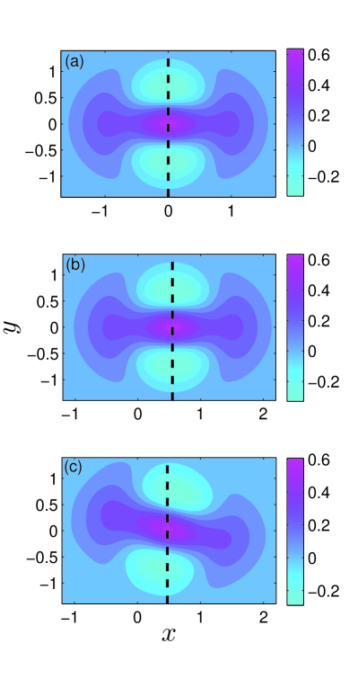
Figure 6: Wigner functions (a) $\mathcal{W}_{c}^{I}\left(\beta,\beta^{\ast}\right)$, (b) $\mathcal{W}_{c}^{D}\left(\beta,\beta^{\ast}\right)$, (c) $\mathcal{W}_{c}^{A}\left(\beta,\beta^{\ast}\right)$ respectively for (a) $\rho_{c}^{I}$, (b) $\rho_{c}^{D}$, and (c) $\rho_{c}^{A}$. Here $x=\operatorname{Re}\left(\beta\right)$, and $y=\operatorname{Im}\left(\beta\right).$ In the above figures, the parameters are chosen as $\omega_{z}/2\pi=19.5\operatorname{GHz}$, $\omega_{x}=1.6\operatorname{GHz}$, $\omega=2\operatorname{GHz}$, $\gamma_{21}/2\pi=\kappa/2\pi=1\operatorname{MHz}$, $\gamma_{11}=0$, $\gamma_{22}=0.1\operatorname{MHz}$, $\eta=\eta_{m}=$ $1.11$, and $x_{d}=x_{d}^{m}=$ $1.305$. We have used a vertical dashed line in (a), (b), and (c) to highlight the displacement of the central point, also the maximum point, of the Wigner functions. As shown in (a), the central point of $\mathcal{W}_{c}^{I}\left(\beta,\beta^{\ast}\right)$ is the origin. Since $\rho_{c}^{D}=D\!\left(\eta_{m}/2\right)\rho_{c}^{I}\>D^{\dagger}\!\left(\eta_{m}/2\right)$, the Wigner function for $\rho_{c}^{D}$, $\mathcal{W}_{c}^{D}\left(\beta,\beta^{\ast}\right)$ and that for $\rho_{c}^{I}$, $\mathcal{W}_{c}^{I}\left(\beta,\beta^{\ast}\right)$ have the relation $\mathcal{W}_{c}^{D}\left(\beta,\beta^{\ast}\right)=\mathcal{W}_{c}^{I}(\beta-\eta_{m}/2,\beta^{\ast}-\eta_{m}/2)$. This is the very reason why (a) and (b) exhibit the same profile as well as a horizonal translation. The exact value of this translation length is, of course, $\eta_{m}/2=0.555$. Compared to the ideal target state in the original picture, i.e., $\mathcal{W}_{c}^{D}\left(\beta,\beta^{\ast}\right)$ in (b), the actual target state $\mathcal{W}_{c}^{A}\left(\beta,\beta^{\ast}\right)$ in (c) possesses nearly the same central point. But due to the effects of environment and unwanted terms, there appears, in (c), a new feature of small local twists and a global rotation.

VI Discussions

Let us now discuss the feasibility of the experiments for the generation of nonclassical microwave states using superconducting quits interacting with a single-mode microwave field. The frequency of the qubit cannot be extremely large. Thus the maximum photon number in multiphoton processes is limited by the ratio $\omega_{z}/\omega$, between the frequency $\omega_{z}$ of the qubit and that of the cavity field $\omega$. This means that the qubits should be far away from the optimal point for the flux and charge qubits when the microwave states are generated using our proposed methods. This might be a problem for the preparation of arbitrary superpositions, because the coherence time becomes short when the flux or charge qubit deviates from the optimal point. However, for the particular number state $\left|n\right\rangle$, there is no requirement for the coherence and thus it should be more efficient, because we need only to prepare the qubit in the excited state, and then the state $\left|n\right\rangle$ can be prepared via an $n$-photon red-sideband excitation. We know that the phase martinis1 ; martinis2 and Xmon Xmon qubits are not very sensitive to the optimal point. Thus the proposal might be more efficient for these qubis coupled to a microwave cavity. It should be noted that the imperfect pulse can significantly affect the fidelity. We thus suggest that enough optimization be implemented to reach an acceptable fidelity.

VII conclusions

We have proposed a method to prepare nonclassical microwave states via longitudinal-coupling-induced multi-photon processes when a driven symmetry-broken superconducting qubit is coupled to a single-mode microwave field. With controllable $k$-photon processes in a SQ with a symmetry-broken potential energy, only $n_{\max}+1$ steps are needed to synthesize the superposition of Fock states with the largest photon number $n_{\max}$. However, in contrast to the method used in Refs. liuepl ; martinis2 , with one-photon processes in the SQ inside the cavity, $2n_{\mathrm{max}}$ steps are needed to synthesize the same state. Moreover, using $k$-photon processes, a $k$-photon Fock state $\left|k\right\rangle$ can be generated with just two steps, while with one-photon processes, $2k$ steps are required to produce the same state. Thus, the time to generate the same state using multiphoton processes is shorter than that using only a single-photon process. Therefore the fidelity should also be improved. In this sense, our method is more efficient than the one in Refs. liuepl ; martinis2 . Besides, we have provided an analytical solution for the total time needed to generate a target state $\left|\psi_{n_{\max}}\right\rangle$.

We have made a detailed analysis of the ground state when the system is sufficiently cooled. We find that in the highly-symmetry-broken and strong-coupling case, the ground state can still be regarded as the vacuum state in the displacement picture. The displacement effect on both the initial state and the target state has also been studied. Generally, the displacement will induce a variation of the photon-number distribution. But in the representation of the Wigner function, its influence is just a shift of the center of the Wigner function by the Lamb-Dicke parameter $\eta=2g/\omega$ between the coupling strength $g$ of the cavity field to the qubit and the frequency $\omega$ of the cavity field. We note that the Fock state produced in the displacement picture is a displaced number state in the original picture. Thus, a circuit QED system with broken symmetry in the qubit potential energy can be used to easily generate a displaced number state. This can be used to study the boundary between the classical and quantum worlds Fink ; Fedorov ; NoriQuanClass2008 ; NoriQCPRB2008 .

In summary, although we find that the nonclassical photon state can be more easily produced when the symmetry of the potential energy of the SQ is broken, this method can be applied to any device with longitudinal and transverse couplings to two-level systems. Although the Fock state can be produced in any symmetry-broken qubit, the superposition of Fock states might be easily realizable in a circuit QED system formed by a phase qubit and a cavity field. This is because phase qubits have no optimal point, and thus not sensitive to the working point of the external parameter. Our proposal is experimentally realizable with current technology.

VIII Acknowledgements

YXL is supported by the National Basic Research Program of China Grant No. 2014CB921401, the NSFC Grants No. 61025022, and No. 91321208. FN is partially supported by the RIKEN iTHES Project, MURI Center for Dynamic Magneto-Optics, and a Grant-in-Aid for Scientific Research (S).

Appendix A Detailed steps for generating the nonclassical state

If we substitute Eq. (24), Eq. (26), and Eq. (32) into Eq. (31), then the following relations can be obtained, e.g., for the generation of $\left|\psi_{0}\right\rangle$, i.e., for the step $n=0$,

$$C_{0g}^{\left(0\right)} =\exp\left(i\alpha_{0g}^{\left(0\right)}\right)\cos\left(\left|\Omega_{N,c}^{0,0}\right|t_{0}\right)C_{0g}^{\left(-1\right)},$$ (57)

$$C_{0e}^{\left(0\right)} =\exp\left(i\alpha_{0e}^{\left(0\right)}\right)\mathrm{sin}\left(\left|\Omega_{N,c}^{0,0}\right|t_{0}\right)C_{0g}^{\left(-1\right)},$$ (58)

with $|C_{0g}^{\left(-1\right)}|=1$, which is determined by the initial condition. However, for the generation of $\left|\psi_{n}\right\rangle$ with $n\geq 1$ from the state $\left|\psi_{n-1}\right\rangle$, we can obtain the following relations for their coefficients

$$C_{kg}^{(n)} =\exp\left(i\alpha_{kg}^{n}\right)C_{kg}^{\left(n-1\right)},$$ (59)

$$C_{ng}^{(n)} =\exp\left(i\alpha_{ng}^{n}\right)\mathrm{sin}\left(\left|\Omega_{N,r}^{n,0}\right|t_{n}\right)C_{0e}^{\left(n-1\right)},$$ (60)

$$C_{0e}^{(n)} =\exp\left(i\alpha_{0e}^{n}\right)\cos\left(\left|\Omega_{N,r}^{n,0}\right|t_{n}\right)C_{0e}^{\left(n-1\right)},$$ (61)

with $k\leq n-1$. Here, the phases $\alpha_{0g}^{(0)}$ and $\alpha_{0e}^{(0)}$ for $n=0$ are determined by

$$\alpha_{0g}^{\left(0\right)} =\frac{x_{d}}{2}\mathrm{sin}\left(\omega_{d}^{\left(0\right)}t_{0}+\phi_{d}^{\left(0\right)}\right)-\frac{x_{d}}{2}\mathrm{sin}\left(\phi_{d}^{\left(0\right)}\right)+\frac{\omega_{z}t_{0}}{2},$$ (62)

$$\alpha_{0e}^{\left(0\right)} =-\frac{x_{d}}{2}\mathrm{sin}\left(\omega_{d}^{\left(0\right)}t_{0}+\phi_{d}^{\left(0\right)}\right)-\frac{x_{d}}{2}\mathrm{sin}\left(\phi_{d}^{\left(0\right)}\right)-\frac{\omega_{z}t_{0}}{2}$$

$$+\phi_{0}-\frac{\pi}{2}.$$ (63)

The other phases with for $n\geq 1$ are given by

$$\alpha_{kg}^{\left(n\right)} =\frac{x_{d}}{2}\mathrm{sin}\left(\omega_{d}^{\left(n\right)}t_{n}+\phi_{d}^{\left(n\right)}\right)-\frac{x_{d}}{2}\mathrm{sin}\left(\phi_{d}^{\left(n\right)}\right)+\frac{\omega_{z}t_{n}}{2}$$

$$-k\omega t_{n},$$ (64)

$$\alpha_{ng}^{\left(n\right)} =\frac{x_{d}}{2}\mathrm{sin}\left(\omega_{d}^{\left(n\right)}t_{n}+\phi_{d}^{\left(n\right)}\right)+\frac{x_{d}}{2}\mathrm{sin}\left(\phi_{d}^{\left(n\right)}\right)+\frac{\omega_{z}t_{n}}{2}$$

$$-n\omega t_{n}-\phi_{n}-\frac{\pi}{2},$$ (65)

$$\alpha_{0e}^{\left(n\right)} =-\frac{x_{d}}{2}\mathrm{sin}\left(\omega_{d}^{\left(n\right)}t_{n}+\phi_{d}^{\left(n\right)}\right)+\frac{x_{d}}{2}\mathrm{sin}\left(\phi_{d}^{\left(n\right)}\right)-\frac{\omega_{z}t_{n}}{2},$$ (66)

where $k\leq n-1.$ In Eqs. (57-61),

$$\phi_{n}=\left\{\begin{array}[c]{ll}\arg\left(\Omega_{N,c}^{0,0}\right)=N\phi_{d}^{\left(n\right)}-\pi,&\ \ \ n=0,\\ \arg\left(\Omega_{N,r}^{n,0}\right)=N\phi_{d}^{\left(n\right)}-\left(n+1\right)\pi,&\ \ \ n\geq 1,\end{array}\right.$$ (67)

if we select an $N$ and $x_{d}$ such that $J_{N}\left(x_{d}\right)<0$, and

$$\phi_{n}=\left\{\begin{array}[c]{ll}\arg\left(\Omega_{N,c}^{0,0}\right)=N\phi_{d}^{\left(n\right)},&\ \ \ n=0,\\ \arg\left(\Omega_{N,r}^{n,0}\right)=N\phi_{d}^{\left(n\right)}-n\pi,&\ \ \ n\geq 1,\end{array}\right.$$ (68)

if we select an $N$ and $x_{d}$ such that $J_{N}\left(x_{d}\right)>0$. Here, $\omega_{d}^{\left(n\right)},$ $\phi_{d}^{\left(n\right)},$ and $t_{n}$ are, respectively, the driving frequency, driving phase, and time duration for each generation step. From Eq. (59), we know that

$$\left|C_{k0}^{\left(n\right)}\right|=\left|C_{k0}^{\left(n_{\max}\right)}\right|=\left|C_{k}\right|,\ \ \ k\leq n.$$ (69)

and hence

$$\left|C_{0e}^{\left(n-1\right)}\right|=\left(1-\sum_{k=0}^{n-1}\left|C_{kg}^{\left(n-1\right)}\right|^{2}\right)^{1/2}=\left(\sum_{k=n}^{n_{\max}}\left|C_{k}\right|^{2}\right)^{1/2}.$$ (70)

Then, from Eqs. (57, 58) and Eqs. (60, 61), we respectively have

$$\left|\Omega_{N,c}^{0,0}\right|t_{0} =\arccos\left|\frac{C_{0g}^{\left(0\right)}}{C_{0g}^{\left(-1\right)}}\right|+2l\pi$$

$$=\arccos\left|C_{0g}^{\left(0\right)}\right|+2l\pi,$$ (71)

$$\left|\Omega_{N,r}^{n,0}\right|t_{n} =\arcsin\left(\frac{\left|C_{ng}^{\left(n\right)}\right|}{\left|C_{0e}^{(n-1)}\right|}\right)+2l\pi$$

$$=\arcsin\left[\frac{\left|C_{n}\right|}{\left(\sum_{k=n}^{n_{\max}}\left|C_{k}\right|^{2}\right)^{1/2}}\right]+2l\pi.$$ (72)

where $l$ is an arbitrary integer. Using Eqs. (57, 58) and Eqs. (60, 61), we derive

$$\arg\left(C_{0g}^{\left(0\right)}\right)-\arg\left(C_{0e}^{\left(0\right)}\right) =\alpha_{0g}^{\left(0\right)}-\alpha_{0e}^{\left(0\right)}+2l\pi,$$ (73)

$$\arg\left(C_{ng}^{\left(n\right)}\right)-\arg\left(C_{0e}^{\left(n\right)}\right) =\alpha_{ng}^{\left(n\right)}-\alpha_{0e}^{\left(n\right)}+2l\pi.$$ (74)

If $n=n_{\max}$ in Eq. (74), then $C_{0e}^{\left(n\right)}=0$, with no definition of the phase angle. Thus we can assume that $\arg\left(C_{0e}^{\left(n\right)}\right)=0$, without affecting the final result. Here, $C_{ng}^{\left(n\right)}$ and $C_{0e}^{\left(n\right)}$ can be obtained through the following recursion relations

$$C_{0e}^{\left(n-1\right)} =\left\{\begin{array}[c]{ll}\frac{C_{0e}^{\left(n\right)}}{\exp\left(i\alpha_{0e}^{\left(n\right)}\right)\cos\left(\left|\Omega_{N,r}^{n,0}\right|t_{n}\right)},&1\leq n<n_{\max},\\ \\ \frac{C_{ng}^{\left(n\right)}}{\exp\left(i\alpha_{ng}^{\left(n\right)}\right)\mathrm{sin}\left(\left|\Omega_{N,r}^{n,0}\right|t_{n}\right)},&n=n_{\max},\end{array}\right.$$ (78)

$$C_{kg}^{\left(n-1\right)} =\frac{C_{kg}^{\left(n\right)}}{\exp\left(i\alpha_{kg}^{\left(n\right)}\right)},k\leq n-1,$$ (79)

$$C_{0g}^{\left(-1\right)} =\frac{C_{0e}^{\left(0\right)}}{\exp\left(i\alpha_{0e}^{\left(0\right)}\right)\mathrm{sin}\left(\left|\Omega_{N,c}^{0,0}\right|t_{0}\right)}.$$ (80)

In Eq. (78), distinguishing the case when $n=n_{\max}$ from the other ones is needed to avoid the apperance of $0/0.$ Though Eq. (80) implies that $C_{0g}^{\left(-1\right)}$ may have a definite phase, such a phase could only add a global phase factor to the target state. So it is convenient to directly specify $C_{0g}^{\left(-1\right)}=1$.

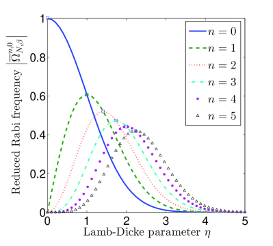
Figure 7: (color online) Reduced Rabi frequency $\left|\bar{\Omega}_{N,\beta}^{n,0}\right|$, from Eq. (81), as a function of $\eta$, for $n=1,2,3,4$, and $5$, respectively. The square on each plot denotes the point that achieves the largest $\left|\bar{\Omega}_{N,\beta}^{n,0}\right|$. Recall that $\eta=2g/\omega$, where $g$ is the qubit-cavity coupling constant and $\omega$ is the frequency of the single-mode cavity field. Thus, $\eta$ is the normalized coupling.

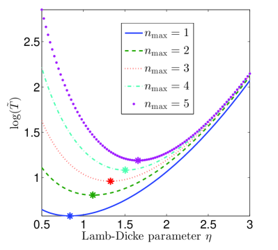
Figure 8: (color online) Plot of $\log\left(\tilde{T}\right)$ as a function of the Lamb-Dicke parameter $\eta=2g/\omega$ for $\left|\psi_{n_{\max}}\right\rangle=\sum_{n=0}^{n_{\max}}\left|n\right\rangle\bigotimes\left|0\right\rangle/\sqrt{n_{\max}+1}$, with different maximum photon number $n_{\max}$. Recall that $\tilde{T}=T\left|\omega J_{N}\right|/2$ is a normalized time and $T$ is the total time to generate the desired target state. The star on each curve shows the optimal point where the normalized generation time reaches its minimum.

We define the reduced Rabi frequency as

$$\left|\bar{\Omega}_{N,\beta}^{n,0}\right|=\frac{2\left|\Omega_{N,\beta}^{n,0}\right|}{\left|\omega_{x}J_{N}\right|}=\exp\left(-\frac{1}{2}\eta^{2}\right)\frac{\eta^{n}}{\sqrt{n!}}$$ (81)

in order to study its dependence on $\eta$. From Eq. (81), we can obtain the optimal Lamb-Dicke parameter

$$\eta_{n,\mathrm{o}}=\sqrt{n},$$ (82)

that achieves the largest reduced Rabi frequency

$$\left|\bar{\Omega}_{N,\beta,\mathrm{o}}^{n,0}\right|=\exp\left(-\frac{n}{2}\right)\frac{n^{n/2}}{\sqrt{n!}},$$ (83)

which is also the point that makes $\left|\bar{\Omega}_{N,\beta}^{0,n}\right|=\left|\bar{\Omega}_{N,\beta}^{0,n-1}\right|$, as illustrated in Fig. 7. We can also verify

$$\lim_{n\rightarrow\infty}\frac{\left|\bar{\Omega}_{N,\beta,\mathrm{o}}^{n+1,0}\right|}{\left|\bar{\Omega}_{N,\beta,\mathrm{o}}^{n,0}\right|}=\lim_{n\rightarrow\infty}\sqrt{\frac{1}{e}\left(\frac{n+1}{n}\right)^{n}}=1,$$ (84)

with $\lim_{n\rightarrow\infty}\left\{\eta_{n+1,\mathrm{o}}/\eta_{n,\mathrm{o}}\right\}=1$. This means that when the photon number $n$ increases, the optimal points for the Rabi frequencies between the zero-photon state and different $n$ photon states tend to approach each other infinitesimally. But for low photon numbers the optimal points are still distinguishable from each other.

Let us calculate the total time $T$ for generating the target state

$$T =\sum_{n=0}^{n_{\max}}t_{n}=\frac{2}{\left|\omega_{x}J_{N}\right|}\arccos\left(\left|C_{0}\right|\right)\exp\left(\frac{\eta^{2}}{2}\right)$$

$$+\sum_{n=1}^{n_{\max}}\frac{2\sqrt{n!}}{\left|\omega_{x}J_{N}\right|\eta^{n}}\arcsin\left(\frac{\left|C_{n}\right|}{\sqrt{\sum_{k=n}^{n_{\max}}\left|C_{k}\right|^{2}}}\right)\exp\left(\frac{\eta^{2}}{2}\right),$$ (85)

where $\eta=2g/\omega$ is the Lamb-Dicke parameter and we have omitted excessive cycle periods for each step. By taking the derivative of $T$ with respect to $\eta,$ we can find all the extreme points of $\eta$, which satisfy the following equation

$$\sum_{n=-1}^{n_{\max}+1}A_{n}\eta^{n_{\max}+1-n}=0.$$ (86)

The coefficient $A_{n}$ has been given in Eqs. (90)-(93). Further selection among these extreme points and the experimentally-constrained boundaries of $\eta$ can yield the optimal Lamb-Dicke parameter $\eta_{\mathrm{opt}}$, which will lead to the least generation time $T_{\mathrm{opt}}$. Once $T_{\mathrm{opt}}$ is reached, in principle, the influence of the environment on the target state fidelity will be minimized.

Similarly to $\left|\bar{\Omega}_{N,\beta}^{0,n}\right|$, we define

$$\tilde{T}\left(\eta\right)=T\left|\omega_{x}J_{N}\right|/2.$$ (87)

The curves of $\log\left(\tilde{T}\left(\eta\right)\right)$ which for particular states have been plotted in Fig. 8 with a star on each curve to label the point where the generation time reaches its least value.

The normalized time needed to generate a target state is

$$\tilde{T} =\sum_{n=0}^{n_{\max}}\tilde{t}_{n}=\arccos\left(\left|C_{0}\right|\right)\exp\left(\eta^{2}/2\right)$$

$$+\sum_{n=1}^{n_{\max}}\sqrt{n!}\arcsin\left(\frac{\left|C_{n}\right|}{\sqrt{\sum_{k=n}^{n_{\max}}\left|C_{k}\right|^{2}}}\right)\frac{e^{\eta^{2}/2}}{\eta^{n}},$$ (88)

whose extreme points still satisfy

$$\sum_{n=-1}^{n_{\max}+1}A_{n}\>\eta^{n_{\max}+1-n}=0,$$ (89)

for unbound $\eta$, where if $n_{\max}=0$,

$$A_{n}=\left\{\begin{array}[c]{ll}\arccos\left(\left|C_{0}\right|\right),&n=-1,\\ 0,&\mathrm{others,}\end{array}\right.$$ (90)

if $n_{\max}=1,$

$$A_{n}=\left\{\begin{array}[c]{ll}\arccos\left(\left|C_{0}\right|\right),&n=-1,\\ P_{n+1},&n=0,\\ -\left(n-1\right)P_{n-1},&n=2,\\ 0,&\mathrm{others,}\end{array}\right.$$ (91)

if $n_{\max}=2$,

$$A_{n}=\left\{\begin{array}[c]{ll}\arccos\left(\left|C_{0}\right|\right),&n=-1,\\ P_{n+1},&0\leq n\leq 1,\\ -\left(n-1\right)P_{n-1},&2\leq n\leq 3,\\ 0,&\mathrm{others,}\end{array}\right.$$ (92)

and for other cases, we have

$$A_{n}=\left\{\begin{array}[c]{ll}\arccos\left(\left|C_{0}\right|\right),&n=-1,\\ P_{n+1},&0\leq n\leq 1,\\ P_{n+1}-\left(n-1\right)P_{n-1},&2\leq n\leq n_{\max}-1,\\ -\left(n-1\right)P_{n-1},&n_{\max}\leq n\leq n_{\max}+1,\\ 0,&\mathrm{others.}\end{array}\right.$$ (93)

Here we have used the abbreviation

$$P_{n}=\sqrt{n!}\arcsin\left(\frac{\left|C_{n}\right|}{\sqrt{\sum_{k=n}^{n_{\max}}\left|C_{k}\right|^{2}}}\right).$$ (94)

References

- (1) Y. Makhlin, G. Schön, and A. Shnirman, Rev. Mod. Phys. 73, 357 (2001).
- (2) J. Q. You and F. Nori, Phys. Today 58 (11), 42 (2005).
- (3) R. J. Schoelkopf and S. M. Girvin, Nature 451, 664 (2008).
- (4) G. Wendin and V. S. Shumeiko, in Handbook of Theoretical and Computational Nanotechnology, edited by M. Rieth and W. Schommers (American Scientific, California, 2006), Vol. 3.
- (5) J. Clarke and F. K. Wilhelm, Nature 453, 1031 (2008).
- (6) J. You and F. Nori, Nature 474, 589 (2011).
- (7) I. Buluta, S. Ashhab, and F. Nori, Rep. Prog. Phys. 74, 104401 (2011).
- (8) Z. L. Xiang, S. Ashhab, J. Q. You, and F. Nori, Rev. Mod. Phys. 85, 623 (2013).
- (9) J. M. Martinis, S. Nam, J. Aumentado, and C. Urbina, Phys. Rev. Lett. 89, 117901 (2002).
- (10) J. Lisenfeld, A. Lukashenko, M. Ansmann, J. M. Martinis, and A. V. Ustinov, Phys. Rev. Lett. 99, 170504 (2007).
- (11) Y. X. Liu, J. Q. You, L. F. Wei, C. P. Sun, and F. Nori, Phys. Rev. Lett. 95, 087001 (2005).
- (12) Y. X. Liu, C.-X. Yang, H.-C. Sun, and X.-B. Wang, New J. Phys. 16, 015031 (2014).
- (13) L. Garziano, R. Stassi, A. Ridolfo, O. Di Stefano, and S. Savasta, Phys. Rev. A 90, 043817 (2014).
- (14) L. Garziano, R. Stassi, A. Ridolfo, O. Di Stefano, and S. Savasta, arXiv:1406.5119 (2014).
- (15) F. Deppe, M. Mariantoni, E. P. Menzel, A. Marx, S. Saito, K. Kakuyanagi, H. Tanaka, T. Meno, K. Semba, H. Takayanagi, E. Solano, and R. Gross, Nature Phys. 4, 686 (2008); T. Niemczyk, F. Deppe, M. Mariantoni, E. P. Menzel, E. Hoffmann, G. Wild, L. Eggenstein, A. Marx, and R. Gross, Supercond. Sci. Technol. 22, 034009 (2009).
- (16) Y. X. Liu, C. P. Sun, and F. Nori, Phys. Rev. A 74, 052321 (2006).
- (17) Ya. S. Greenberg, Phys. Rev. B 76, 104520 (2007).
- (18) C. M. Wilson, T. Duty, F. Persson, M. Sandberg, G. Johansson, and P. Delsing, Phys. Rev. Lett. 98, 257003 (2007); C. M. Wilson, G. Johansson, T. Duty, F. Persson, M. Sandberg, and P. Delsing, Phys. Rev. B 81, 024520 (2010).
- (19) J. M. Fink, R. Bianchetti, M. Baur, M. Goppl, L. Steffen, S. Filipp, P. J. Leek, A. Blais, and A. Wallraff, Phys. Rev. Lett. 103, 083601 (2009).
- (20) K. V. R. M. Murali, Z. Dutton, W. D. Oliver, D. S. Crankshaw, and T. P. Orlando, Phys. Rev. Lett. 93, 087003 (2004); Z. Dutton, K. V. R. M. Murali, W. D. Oliver, and T. P. Orlando, Phys. Rev. B 73, 104516 (2006).
- (21) X. Z. Yuan, H. S. Goan, C. H. Lin, K. D. Zhu, and Y. W. Jiang, New J. Phys. 10, 095016 (2008).
- (22) H. Ian, Y. X. Liu, and F. Nori, Phys. Rev. A 81, 063823 (2010).
- (23) J. Siewert, T. Brandes, and G. Falci, Phys. Rev. B 79, 024504 (2009).
- (24) J. Joo, J. Bourassa, A. Blais, and B. C. Sanders, Phys. Rev. Lett. 105, 073601 (2010).
- (25) H.-C. Sun, Y. X. Liu, H. Ian, J. Q. You, E. Il’ichev, and F. Nori, Phys. Rev. A 89, 063822 (2014).
- (26) B. Peng, Ş. K. Özdemir, W. Chen, F. Nori, and L. Yang, Nat. Commun. 5, 5082 (2014).
- (27) M. Baur, S. Filipp, R. Bianchetti, J. M. Fink, M. Göppl, L. Steffen, P. J. Leek, A. Blais, and A. Wallraff, Phys. Rev. Lett. 102, 243602 (2009).
- (28) M. A. Sillanpää, J. Li, K. Cicak, F. Altomare, J. I. Park, R. W. Simmonds, G. S. Paraoanu, and P. J. Hakonen, Phys. Rev. Lett. 103, 193601 (2009); J. Li, G. S. Paraoanu, K. Cicak, F. Altomare, J. I. Park, R. W. Simmonds, M. A. Sillanpää, and P. J. Hakonen, Phys. Rev. B 84, 104527 (2011); Sci. Rep. 2, 645 (2012).
- (29) A. A. Abdumalikov, Jr., O. Astafiev, A. M. Zagoskin, Yu. A. Pashkin, Y. Nakamura, and J. S. Tsai, Phys. Rev. Lett. 104, 193601 (2010).
- (30) P. M. Anisimov, J. P. Dowling, and B. C. Sanders, Phys. Rev. Lett. 107, 163604 (2011).
- (31) I.-C. Hoi, C. M. Wilson, G. Johansson, J. Lindkvist, B. Peropadre, T. Palomaki, and P. Delsing, New J. Phys. 15, 025011 (2013).
- (32) S. Novikov, J. E. Robinson, Z. K. Keane, B. Suri, F. C. Wellstood, and B. S. Palmer, Phys. Rev. B 88, 060503(R) (2013).
- (33) W. R. Kelly, Z. Dutton, J. Schlafer, B. Mookerji, and T. A. Ohki, J. S. Kline, and D. P. Pappas, Phys. Rev. Lett. 104, 163601 (2010).
- (34) S. O. Valenzuela, W. D. Oliver, D. M. Berns, K. K. Berggren, L. S. Levitov, and T. P. Orlando, Science 314, 1589 (2006).
- (35) J. Q. You, Y. X. Liu, and F. Nori, Phys. Rev. Lett. 100, 047001 (2008).
- (36) F. Nori, Nat. Phys. 4, 589 (2008).
- (37) M. Grajcar, S. H. W. van der Ploeg, A. Izmalkov, E. Il’ichev, H.-G. Meyer, A. Fedorov, A. Shnirman, and G. Schon, Nature Phys. 4, 612 (2008).
- (38) Y. X. Liu, L. F. Wei, J. R. Johansson, J. S. Tsai, and F. Nori, Phys. Rev. B 76, 144518 (2007).
- (39) J. Q. You and F. Nori, Phys. Rev. B 68, 064509 (2003).
- (40) J. Q. You, J. S. Tsai, and F. Nori, Phys. Rev. B 68, 024510 (2003).
- (41) A. Blais, J. Gambetta, A. Wallraff, D. I. Schuster, S. M. Girvin, M. H. Devoret, and R. J. Schoelkopf, Phys. Rev. A 75, 032329 (2007).
- (42) A. Wallraff, D. I. Schuster, A. Blais, J. M. Gambetta, J. Schreier, L. Frunzio, M. H. Devoret, S. M. Girvin, and R. J. Schoelkopf, Phys. Rev. Lett. 99, 050501 (2007).
- (43) P. J. Leek, S. Filipp, P. Maurer, M. Baur, R. Bianchetti, J. M. Fink, M. Göppl, L. Steffen, and A. Wallraff, Phys. Rev. B 79, 180511(R) (2009).
- (44) M. Sasura and V. Buzek, J. Mod. Opt. 49, 1593 (2002).
- (45) L. Wei, Y. X. Liu, and F. Nori, Phys. Rev. A 70, 063801 (2004).
- (46) Y. X. Liu, L. F. Wei, J. R. Johansson, J. S. Tsai, and F. Nori, Phys. Rev. B 76, 144518 (2007).
- (47) S. Ashhab, J. R. Johansson, A. M. Zagoskin, and F. Nori, Phys. Rev. A 75, 063414 (2007).
- (48) S. N. Shevchenko, S. Ashhab, and F. Nori, Phys. Rep. 492, 1 (2010).
- (49) S. Saito, M. Thorwart, H. Tanaka, M. Ueda, H. Nakano, K. Semba, and H. Takayanagi, Phys. Rev. Lett. 93, 037001 (2004).
- (50) A. Izmalkov, M. Grajcar, E. Il’ichev, N. Oukhanski, T. Wagner, H.-G. Meyer, W. Krech, M. H. S. Amin, A. Maassen van den Brink, and A. M. Zagoskin, Europhys. Lett. 65, 844 (2004).
- (51) W. D. Oliver, Y. Yu, J. C. Lee, K. K. Berggren, L. S. Levitov, and T. P. Orlando, Science 310, 1653 (2005).
- (52) D. M. Berns, W. D. Oliver, S. O. Valenzuela, A. V. Shytov, K. K. Berggren, L. S. Levitov, and T. P. Orlando, Phys. Rev. Lett. 97, 150502 (2006).
- (53) X. Wen and Y. Yu, Phys. Rev. B 79, 094529 (2009).
- (54) A. Blais, R.-S. Huang, A. Wallraff, S. M. Girvin, and R. J. Schoelkopf, Phys. Rev. A 69, 062320 (2004).
- (55) A. Wallraff, D. I. Schuster, A. Blais, L. Frunzio, R. S. Huang, J. Majer, S. Kumar, S. M. Girvin, and R. J. Schoelkopf, Nature 431, 162 (2004).
- (56) I. Chiorescu, P. Bertet, K. Semba, Y. Nakamura, C. J. P. M. Harmans, and J. E. Mooij, Nature 431, 159 (2004).
- (57) M. N. Nielsen and I. L. Chuang, Quantum Computation and Quantum Information (Cambridge University Press 2000).
- (58) Y. X. Liu, L. F. Wei, and F. Nori, Europhys. Lett. 67, 941 (2004).
- (59) Y. X. Liu, L. F. Wei, and F. Nori, Phys. Rev. A 71, 063820 (2005).
- (60) M. Hofheinz, E. M. Weig, M. Ansmann, R. C. Bialczak, E. Lucero, M. Neeley, H. Wang, J. M. Martinis, and A. N. Cleland, Nature (London) 454, 310 (2008).
- (61) M. Hofheinz, H. Wang, M. Ansmann, R. C. Bialczak, E. Lucero, M. Neeley, A. D. O’Connell, D. Sank, J. Wenner, J. M. Martinis, and A. N. Cleland, Nature (London) 459, 546 (2009).
- (62) M. O. Scully and M. S. Zubairy, Quantum Optics (Cambridge University Press, Cambridge, England, 1997).
- (63) F. A. M. de Oliveira, M. S. Kim, P. L. Knight, and V. Buek, Phys. Rev. A 41, 2645 (1990).
- (64) D. Leibfried, D. M. Meekhof, B. E. King, C. Monroe, W. M. Itano, and D. J. Wineland, Phys. Rev. Lett. 77, 4281 (1996).
- (65) C. Eichler, D. Bozyigit, C. Lang, M. Baur, L. Steffen, J. M. Fink, S. Filipp, and A. Wallraff, Phys. Rev. Lett. 107, 113601 (2011).
- (66) Y. Shalibo, R. Resh, O. Fogel, D. Shwa, R. Bialczak, J. M. Martinis, and N. Katz, Phys. Rev. Lett. 110, 100404 (2013).
- (67) G. S. Agarwal and K. Tara, Phys. Rev. A 43, 492 (1991).
- (68) W. H. Louisell, Quantum Statistical Properties of Radiation (Wiley, Canada, 1973).
- (69) C. W. Gardiner and P. Zoller, Quantum Noise: A Handbook of Markovian and Non-Markovian Quantum Stochastic Methods with Applications to Quantum Optics (Springer, 2000).
- (70) R. Barends, J. Kelly, A. Megrant, D. Sank, E. Jeffrey, Y. Chen, Y. Yin, B. Chiaro, J. Mutus, C. Neill, P. O’Malley, P. Roushan, J. Wenner, T. C. White, A. N. Cleland, and John M. Martinis, Phys. Rev. Lett. 111, 080502 (2013).
- (71) T. Niemczyk, F. Deppe, H. Huebl, E. Menzel, F. Hocke, M. Schwarz, J. Garcia-Ripoll, D. Zueco, T. Hümmer, and E. Solano, Nat. Phys. 6, 772 (2010).
- (72) P. Forn-Díaz, J. Lisenfeld, D. Marcos, J. J. García-Ripoll , E. Solano, C. J. P. M. Harmans, and J. E. Mooij, Phys. Rev. Lett. 105, 237001 (2010).
- (73) R. Stassi, A. Ridolfo, O. Di Stefano, M. J. Hartmann, and S. Savasta, Phys. Rev. Lett. 110, 243601 (2013).
- (74) J. Casanova, G. Romero, I. Lizuain, J. J. García-Ripoll, and E. Solano, Phys. Rev. Lett. 105, 263603 (2010).
- (75) D. Braak, Phys. Rev. Lett. 107, 100401 (2011).
- (76) E. Solano, Physics 4, 68 (2011).
- (77) S. De Liberato, Phys. Rev. Lett. 112, 016401 (2014).
- (78) J. M. Fink, L. Steffen, P. Studer, L. S. Bishop, M. Baur, R. Bianchetti, D. Bozyigit, C. Lang, S. Filipp, P. J. Leek, and A. Wallraff, Phys. Rev. Lett. 105, 163601 (2010).
- (79) A. Fedorov, P. Macha, A. K. Feofanov, C. J. P. M. Harmans, and J. E. Mooij, Phys. Rev. Lett. 106, 170404 (2011).
- (80) S. Shevchenko, A. Omelyanchouk, A. Zagoskin, S. Savel’ev, and F. Nori, New J. Phys. 10, 073026 (2008).
- (81) A. Omelyanchouk, S. Shevchenko, A. Zagoskin, E. Il’ichev, and F. Nori, Phys. Rev. B 78, 054512 (2008).