Robust Bounded Influence Tests for

Independent Non-Homogeneous Observations

Abhik Ghosh and Ayanendranath Basu

Indian Statistical Institute, Kolkata, India

Abstract: Experiments often yield non-identically distributed data for statistical analysis. Tests of hypothesis under such set-ups are generally performed using the likelihood ratio test, which is non-robust with respect to outliers and model misspecification. In this paper, we consider the set-up of non-identically but independently distributed observations and develop a general class of test statistics for testing parametric hypothesis based on the density power divergence. The proposed tests have bounded influence functions, are highly robust with respect to data contamination, have high power against contiguous alternatives, and are consistent at any fixed alternative. The methodology is illustrated by the simple and generalized linear regression models with fixed covariates.

Key words and phrases: Robust Testing of Hypothesis, Non-Homogeneous Observation, Linear Regression, Generalized Linear Model, Influence Function.

1 Introduction

One of the most important paradigms of statistical inference is hypothesis testing; arguably the most common test is the likelihood ratio test (LRT). However, like the maximum likelihood estimator (MLE), the LRT may lead to unstable inference in the presence of outliers. Attempts to rectify this (Simpson (1989); Lindsay (1994); Basu et al. (2013a, b)) have mostly been in the context of independent and identically distributed (i.i.d.) data. In this paper, we consider the general case of non-identically distributed data. Suppose the observed data Y1,,Ynsubscript𝑌1subscript𝑌𝑛Y_{1},\ldots,Y_{n} are independent, but for each i𝑖i, Yigisimilar-tosubscript𝑌𝑖subscript𝑔𝑖Y_{i}\sim g_{i} with g1,,gnsubscript𝑔1subscript𝑔𝑛g_{1},\ldots,g_{n} being possibly different densities with respect to some common dominating measure. We model gisubscript𝑔𝑖g_{i} by the family i,𝜽={fi(;𝜽)|𝜽Θ}subscript𝑖𝜽conditional-setsubscript𝑓𝑖𝜽𝜽Θ{\mathcal{F}}_{i,{\boldsymbol{\theta}}}=\{f_{i}(\cdot;{\boldsymbol{\theta}})|~{}{\boldsymbol{\theta}}\in\Theta\} for all i=1,2,,n𝑖12𝑛i=1,2,\ldots,n. Let Gisubscript𝐺𝑖G_{i} and Fi(,𝜽)subscript𝐹𝑖𝜽F_{i}(\cdot,{\boldsymbol{\theta}}) be the indicated distribution functions. Even though the Yisubscript𝑌𝑖Y_{i}s have possibly different densities, they share the common parameter 𝜽𝜽{\boldsymbol{\theta}}. We will refer to this set-up as the independent non-homogeneous (I-NH) set-up.

The most prominent application of the I-NH set-up is the regression model with non-stochastic covariates, where fisubscript𝑓𝑖f_{i} is a known density depending on the given predictors 𝒙isubscript𝒙𝑖{\boldsymbol{x}_{i}}, error distribution, and a common regression parameter 𝜷𝜷\boldsymbol{\beta}, yifi(,𝒙i,𝜷)similar-tosubscript𝑦𝑖subscript𝑓𝑖subscript𝒙𝑖𝜷y_{i}\sim f_{i}(\cdot,{\boldsymbol{x}_{i}},\boldsymbol{\beta}). This differs from the usual regression set-up with stochastic covariates that has been explored in greater detail in the literature (Ronchetti and Rousseeuw (1980); Schrader and Hettmansperger (1980); Ronchetti (1982a, b, 1987); Sen (1982); Markatou and Hettmansperger (1990); Markatou and He (1994); Markatou and Manos (1996); Cantoni and Ronchetti (2001); Liu et al. (2005); Maronna et al. (2006); Wang and Qu (2007); Hosseinian (2009); Salibian-Barrera et al. (2016)). Our set-up treats the regression problem from a design point of view where we pre-fix the covariate levels. The robustness literature under this general I-NH set-up is limited; some scattered attempts have been made in particular cases like normal regression (Huber (1983); Muller (1998)).

Ghosh and Basu (2013) proposed a global approach for estimating 𝜽𝜽{\boldsymbol{\theta}} under the I-NH set-up by minimizing the average density power divergence (DPD) measure (originally introduced by Basu et al. (1998) for i.i.d. data) between the data and the model density; the proposed minimum DPD estimator (MDPDE) has excellent efficiency and robustness properties in the normal regression model. The approach is also implemented in the context of generalized linear models by Ghosh and Basu (2016); it provides a competitive alternative to existing robust methods. The approach has been used in Ghosh (2017) to obtain a robust alternative for tail index estimation under suitable assumptions of an exponential regression model. Here, we exploit the properties of the Ghosh and Basu (2013) estimator to develop a general class of robust tests of hypotheses for I-NH data.

The specific advantages of the proposed methods are as follows. (1) The method is completely general in that it works for any set-up involving independent and non-homogeneous data. (2) The proposal is simple to implement with minimal addition in computational complexity compared to likelihood based methods. (3) The testing procedure is based on the minimization of a bona-fide objective function and the selection of the proper root of the estimating equation is simple as it must correspond to the global minimum. (4) Our methods have bounded influence for the test statistics, and the level and power influence functions. (5) The proposed tests are consistent at any fixed alternative, and have high power against any contiguous alternative.

In this paper, we assume Conditions (A1)–(A7) of Ghosh and Basu (2013), which we refer to as the “Ghosh-Basu conditions”, and Assumptions A, B, C and D of Lehmann (1983, p. 429), which we refer to as the “Lehmann conditions”. These conditions are listed in Section S1 of the Online Supplement for completeness.

2 The MDPDE under the I-NH Set-up

Under the I-NH set-up, Ghosh and Basu (2013) proposed the estimation of 𝜽𝜽{\boldsymbol{\theta}} by minimizing the average DPD measure between the data and the model, or equivalently

Hn(𝜽)=1ni=1n[fi(y;𝜽)1+τ𝑑y(1+1τ)fi(Yi;𝜽)τ]=1ni=1nVi(Yi;𝜽).subscript𝐻𝑛𝜽1𝑛superscriptsubscript𝑖1𝑛delimited-[]subscript𝑓𝑖superscript𝑦𝜽1𝜏differential-d𝑦11𝜏subscript𝑓𝑖superscriptsubscript𝑌𝑖𝜽𝜏1𝑛superscriptsubscript𝑖1𝑛subscript𝑉𝑖subscript𝑌𝑖𝜽\displaystyle H_{n}({\boldsymbol{\theta}})=\frac{1}{n}\sum_{i=1}^{n}\left[\int f_{i}(y;{\boldsymbol{\theta}})^{1+\tau}dy-\left(1+\frac{1}{\tau}\right)f_{i}(Y_{i};{\boldsymbol{\theta}})^{\tau}\right]=\frac{1}{n}\sum_{i=1}^{n}V_{i}(Y_{i};{\boldsymbol{\theta}}). (2.1)

The corresponding estimating equation is given by

i=1n[fi(Yi;𝜽)τ𝒖i(Yi;𝜽)fi(y;𝜽)1+τ𝒖i(y;𝜽)𝑑y]=0,superscriptsubscript𝑖1𝑛delimited-[]subscript𝑓𝑖superscriptsubscript𝑌𝑖𝜽𝜏subscript𝒖𝑖subscript𝑌𝑖𝜽subscript𝑓𝑖superscript𝑦𝜽1𝜏subscript𝒖𝑖𝑦𝜽differential-d𝑦0\sum_{i=1}^{n}\left[f_{i}(Y_{i};{\boldsymbol{\theta}})^{\tau}\boldsymbol{u}_{i}(Y_{i};{\boldsymbol{\theta}})-\int f_{i}(y;{\boldsymbol{\theta}})^{1+\tau}\boldsymbol{u}_{i}(y;{\boldsymbol{\theta}})dy\right]=0, (2.2)

where \nabla represents the gradient with respect to 𝜽𝜽{\boldsymbol{\theta}}, and 𝒖i(y;𝜽)=lnfi(y;𝜽)subscript𝒖𝑖𝑦𝜽subscript𝑓𝑖𝑦𝜽\boldsymbol{u}_{i}(y;{\boldsymbol{\theta}})=\nabla\ln f_{i}(y;{\boldsymbol{\theta}}) is the likelihood score function for i𝑖i-th model density (Similarly, 2superscript2\nabla^{2} represents the second order derivative with respect to 𝜽𝜽{\boldsymbol{\theta}}). When τ=0𝜏0\tau=0, the MDPDE is seen to coincide with the non-robust maximum likelihood estimator (MLE); as τ𝜏\tau increases the robustness increases significantly at the cost of a slight loss in asymptotic efficiency.

With 𝑮¯=(G1,,Gn)¯𝑮subscript𝐺1subscript𝐺𝑛\underline{\boldsymbol{G}}=(G_{1},\cdots,G_{n}), the minimum DPD functional 𝜽g=𝑼τ(𝑮¯)superscript𝜽𝑔subscript𝑼𝜏¯𝑮{\boldsymbol{\theta}}^{g}=\boldsymbol{U}_{\tau}(\underline{\boldsymbol{G}}) for the I-NH observations is defined by

1ni=1ndτ(gi(.),fi(.;𝑼τ(𝑮¯)))=min𝜽Θ1ni=1ndτ(gi(.),fi(.;𝜽)),\frac{1}{n}\sum_{i=1}^{n}d_{\tau}(g_{i}(.),f_{i}(.;\boldsymbol{U}_{\tau}(\underline{\boldsymbol{G}})))=\min_{{\boldsymbol{\theta}}\in\Theta}\frac{1}{n}\sum_{i=1}^{n}d_{\tau}(g_{i}(.),f_{i}(.;{\boldsymbol{\theta}})), (2.3)

where dτ(f1,f2)subscript𝑑𝜏subscript𝑓1subscript𝑓2d_{\tau}(f_{1},f_{2}) denotes the DPD measure between two densities f1subscript𝑓1f_{1} and f2subscript𝑓2f_{2} with the tuning parameter τ𝜏\tau, as given by Basu et al. (1998),

dτ(f1,f2)={[f21+τ(1+1τ)f2τf1+1τf11+τ],forτ>0,f1log(f1/f2),forτ=0.subscript𝑑𝜏subscript𝑓1subscript𝑓2casesdelimited-[]superscriptsubscript𝑓21𝜏11𝜏superscriptsubscript𝑓2𝜏subscript𝑓11𝜏superscriptsubscript𝑓11𝜏for𝜏0subscript𝑓1subscript𝑓1subscript𝑓2for𝜏0d_{\tau}(f_{1},f_{2})=\displaystyle\left\{\begin{array}[]{ll}\displaystyle\int\left[f_{2}^{1+\tau}-\left(1+\frac{1}{\tau}\right)f_{2}^{\tau}f_{1}+\frac{1}{\tau}f_{1}^{1+\tau}\right],&{\rm for}~{}\tau>0,\\ \displaystyle\int f_{1}\log(f_{1}/f_{2}),&{\rm for}~{}\tau=0.\end{array}\right. (2.4)

Equivalently, 𝑼τ(𝑮¯)subscript𝑼𝜏¯𝑮\boldsymbol{U}_{\tau}(\underline{\boldsymbol{G}}) is the minimizer of 1ni=1nH(i)(𝜽)1𝑛superscriptsubscript𝑖1𝑛superscript𝐻𝑖𝜽\frac{1}{n}\sum_{i=1}^{n}H^{(i)}({\boldsymbol{\theta}}), with respect to 𝜽Θ𝜽Θ{\boldsymbol{\theta}}\in\Theta, where H(i)(𝜽)=fi(y;𝜽)1+τ𝑑y(1+1τ)fi(y;𝜽)τgi(y)𝑑y.superscript𝐻𝑖𝜽subscript𝑓𝑖superscript𝑦𝜽1𝜏differential-d𝑦11𝜏subscript𝑓𝑖superscript𝑦𝜽𝜏subscript𝑔𝑖𝑦differential-d𝑦H^{(i)}({\boldsymbol{\theta}})=\int f_{i}(y;{\boldsymbol{\theta}})^{1+\tau}dy-\left(1+\frac{1}{\tau}\right)\int f_{i}(y;{\boldsymbol{\theta}})^{\tau}g_{i}(y)dy.

Ghosh and Basu (2013) derived the asymptotic distribution of the MDPDE 𝜽^nsubscript^𝜽𝑛\hat{{\boldsymbol{\theta}}}_{n}, under this set-up. Under the Ghosh-Basu conditions, we have the following.
(i) There exists a consistent sequence 𝜽^nsubscript^𝜽𝑛\widehat{{\boldsymbol{\theta}}}_{n} of roots of (2.2).

(ii) The asymptotic distribution of 𝛀nτ(𝜽g)12𝚿nτ(𝜽g)[n(𝜽^n𝜽g)]superscriptsubscript𝛀𝑛𝜏superscriptsuperscript𝜽𝑔12superscriptsubscript𝚿𝑛𝜏superscript𝜽𝑔delimited-[]𝑛subscript^𝜽𝑛superscript𝜽𝑔\boldsymbol{\Omega}_{n}^{\tau}({\boldsymbol{\theta}}^{g})^{-\frac{1}{2}}\boldsymbol{\Psi}_{n}^{\tau}({\boldsymbol{\theta}}^{g})[\sqrt{n}(\widehat{\boldsymbol{\theta}}_{n}-{\boldsymbol{\theta}}^{g})] is p𝑝p-dimensional normal with (vector) mean 𝟎0\boldsymbol{0} and covariance matrix 𝑰psubscript𝑰𝑝\boldsymbol{I}_{p}, the p𝑝p-dimensional identity matrix, where 𝚿nτ(𝜽g)=1ni=1n𝑱(i)(𝜽g),superscriptsubscript𝚿𝑛𝜏superscript𝜽𝑔1𝑛superscriptsubscript𝑖1𝑛superscript𝑱𝑖superscript𝜽𝑔\boldsymbol{\Psi}_{n}^{\tau}({\boldsymbol{\theta}}^{g})=\frac{1}{n}\sum_{i=1}^{n}\boldsymbol{J}^{(i)}({\boldsymbol{\theta}}^{g}), with

𝑱(i)(𝜽g)=superscript𝑱𝑖superscript𝜽𝑔absent\displaystyle\boldsymbol{J}^{(i)}({\boldsymbol{\theta}}^{g})= 𝒖i(y;𝜽g)𝒖iT(y;𝜽g)fi1+τ(y;𝜽g)𝑑ysubscript𝒖𝑖𝑦superscript𝜽𝑔superscriptsubscript𝒖𝑖𝑇𝑦superscript𝜽𝑔superscriptsubscript𝑓𝑖1𝜏𝑦superscript𝜽𝑔differential-d𝑦\displaystyle\int{\boldsymbol{u}_{i}}(y;{\boldsymbol{\theta}}^{g}){\boldsymbol{u}_{i}}^{T}(y;{\boldsymbol{\theta}}^{g})f_{i}^{1+\tau}(y;{\boldsymbol{\theta}}^{g})dy
{𝒖i(y;𝜽g)+τ𝒖i(y;𝜽g)𝒖iT(y;𝜽g)}{gi(y)fi(y;𝜽g)}fi(y;𝜽g)τ𝑑y,subscript𝒖𝑖𝑦superscript𝜽𝑔𝜏subscript𝒖𝑖𝑦superscript𝜽𝑔superscriptsubscript𝒖𝑖𝑇𝑦superscript𝜽𝑔subscript𝑔𝑖𝑦subscript𝑓𝑖𝑦superscript𝜽𝑔subscript𝑓𝑖superscript𝑦superscript𝜽𝑔𝜏differential-d𝑦\displaystyle-\int\{\mathbf{\nabla}{\boldsymbol{u}_{i}}(y;{\boldsymbol{\theta}}^{g})+\tau{\boldsymbol{u}_{i}}(y;{\boldsymbol{\theta}}^{g}){\boldsymbol{u}_{i}}^{T}(y;{\boldsymbol{\theta}}^{g})\}\{g_{i}(y)-f_{i}(y;{\boldsymbol{\theta}}^{g})\}f_{i}(y;{\boldsymbol{\theta}}^{g})^{\tau}dy,
and𝛀nτ(𝜽g)=andsuperscriptsubscript𝛀𝑛𝜏superscript𝜽𝑔absent\displaystyle\mbox{and}~{}~{}~{}\boldsymbol{\Omega}_{n}^{\tau}({\boldsymbol{\theta}}^{g})= 1ni=1n[𝒖i(y;𝜽g)𝒖iT(y;𝜽g)fi(y;𝜽g)2τgi(y)𝑑y𝝃i𝝃iT],1𝑛superscriptsubscript𝑖1𝑛delimited-[]subscript𝒖𝑖𝑦superscript𝜽𝑔superscriptsubscript𝒖𝑖𝑇𝑦superscript𝜽𝑔subscript𝑓𝑖superscript𝑦superscript𝜽𝑔2𝜏subscript𝑔𝑖𝑦differential-d𝑦subscript𝝃𝑖superscriptsubscript𝝃𝑖𝑇\displaystyle\frac{1}{n}\sum_{i=1}^{n}\left[\int{\boldsymbol{u}_{i}}(y;{\boldsymbol{\theta}}^{g}){\boldsymbol{u}_{i}}^{T}(y;{\boldsymbol{\theta}}^{g})f_{i}(y;{\boldsymbol{\theta}}^{g})^{2\tau}g_{i}(y)dy-\boldsymbol{\xi}_{i}\boldsymbol{\xi}_{i}^{T}\right],
with𝝃i=𝒖i(y;𝜽g)fi(y;𝜽g)τgi(y)𝑑y.withsubscript𝝃𝑖subscript𝒖𝑖𝑦superscript𝜽𝑔subscript𝑓𝑖superscript𝑦superscript𝜽𝑔𝜏subscript𝑔𝑖𝑦differential-d𝑦\displaystyle\mbox{with}~{}~{}~{}~{}~{}~{}~{}~{}~{}~{}~{}~{}~{}~{}~{}~{}~{}~{}~{}~{}~{}~{}~{}~{}\boldsymbol{\xi}_{i}=\int{\boldsymbol{u}_{i}}(y;{\boldsymbol{\theta}}^{g})f_{i}(y;{\boldsymbol{\theta}}^{g})^{\tau}g_{i}(y)dy.~{}~{}~{}~{}~{}~{}~{}~{}~{}~{}~{}~{}~{}~{} (2.5)

3 Testing Simple Hypothesis

We start with the simple hypothesis testing problem with a fully specified null under the I-NH set-up. Let 𝜽0subscript𝜽0{\boldsymbol{\theta}}_{0} be a fixed point in the parameter space ΘΘ\Theta. We want to test

H0:𝜽=𝜽0 against H1:𝜽𝜽0.:subscript𝐻0𝜽subscript𝜽0 against subscript𝐻1:𝜽subscript𝜽0H_{0}:{\boldsymbol{\theta}}={\boldsymbol{\theta}}_{0}~{}~{}~{}\mbox{ against }~{}~{}~{}~{}H_{1}:{\boldsymbol{\theta}}\neq{\boldsymbol{\theta}}_{0}. (3.6)

When the model is correctly specified and the null hypothesis is correct, fi(;𝜽0)subscript𝑓𝑖subscript𝜽0f_{i}(\cdot;{\boldsymbol{\theta}}_{0}) is the data generating density for the i𝑖i-th observation. We can test for the hypothesis in (3.6) by using the DPD measure between fi(;𝜽0)subscript𝑓𝑖subscript𝜽0f_{i}(\cdot;{\boldsymbol{\theta}}_{0}) and fi(;𝜽^)subscript𝑓𝑖^𝜽f_{i}(\cdot;\widehat{\boldsymbol{\theta}}) for any estimator 𝜽^^𝜽\widehat{{\boldsymbol{\theta}}} of 𝜽𝜽{\boldsymbol{\theta}}. We consider the MDPDE 𝜽nτsuperscriptsubscript𝜽𝑛𝜏{\boldsymbol{\theta}}_{n}^{\tau} of 𝜽𝜽{\boldsymbol{\theta}} as defined in Section 2. Since there are n𝑛n divergence measures corresponding to each i𝑖i, we consider the total divergence measure over the n𝑛n data points for testing (3.6) and define the DPD based test statistic (DPDTS) as

Tγ(𝜽nτ,𝜽0)=2i=1ndγ(fi(.;𝜽nτ),fi(.;𝜽0)),T_{\gamma}({{\boldsymbol{\theta}}_{n}^{\tau}},{{\boldsymbol{\theta}}_{0}})=2\sum_{i=1}^{n}~{}d_{\gamma}(f_{i}(.;{\boldsymbol{\theta}}_{n}^{\tau}),f_{i}(.;{\boldsymbol{\theta}}_{0})),

where dγ(f1,f2)subscript𝑑𝛾subscript𝑓1subscript𝑓2d_{\gamma}(f_{1},f_{2}) is defined in (2.4). In case of i.i.d. data, this DPDTS coincides with the test statistic in Basu et al. (2013a).

3.1 Asymptotic Properties

Consider the matrices 𝚿nτsuperscriptsubscript𝚿𝑛𝜏\boldsymbol{\Psi}_{n}^{\tau} and 𝛀nτsuperscriptsubscript𝛀𝑛𝜏\boldsymbol{\Omega}_{n}^{\tau} defined in Section 2 and let 𝑨nγ(𝜽)=1ni=1n𝑨γ(i)(𝜽)superscriptsubscript𝑨𝑛𝛾𝜽1𝑛superscriptsubscript𝑖1𝑛superscriptsubscript𝑨𝛾𝑖𝜽\boldsymbol{A}_{n}^{\gamma}({\boldsymbol{\theta}})=\frac{1}{n}\sum_{i=1}^{n}\boldsymbol{A}_{\gamma}^{(i)}({\boldsymbol{\theta}}) with 𝑨γ(i)(𝜽0)=2dγ(fi(.;𝜽),fi(.;𝜽0))|𝜽=𝜽0.\boldsymbol{A}_{\gamma}^{(i)}({\boldsymbol{\theta}}_{0})=\nabla^{2}d_{\gamma}(f_{i}(.;{\boldsymbol{\theta}}),f_{i}(.;{\boldsymbol{\theta}}_{0}))\big{|}_{{\boldsymbol{\theta}}={\boldsymbol{\theta}}_{0}}. For some p×p𝑝𝑝p\times p matrices 𝑱τsubscript𝑱𝜏{\boldsymbol{J}_{\tau}}, 𝑽τsubscript𝑽𝜏{\boldsymbol{V}_{\tau}}, Aτsubscript𝐴𝜏A_{\tau}, and 𝜽Θ𝜽Θ{\boldsymbol{\theta}}\in\Theta, consider the assumptions.

  • (C1)

    𝚿nτ(𝜽)𝑱τ(𝜽)superscriptsubscript𝚿𝑛𝜏𝜽subscript𝑱𝜏𝜽\boldsymbol{\Psi}_{n}^{\tau}({\boldsymbol{\theta}})\rightarrow{\boldsymbol{J}_{\tau}}({\boldsymbol{\theta}}) and 𝛀nτ(𝜽)𝑽τ(𝜽)superscriptsubscript𝛀𝑛𝜏𝜽subscript𝑽𝜏𝜽\boldsymbol{\Omega}_{n}^{\tau}({\boldsymbol{\theta}})\rightarrow{\boldsymbol{V}_{\tau}}({\boldsymbol{\theta}}) element-wise as n𝑛n\rightarrow\infty

  • (C2)

    𝑨nγ(𝜽)𝑨γ(𝜽)superscriptsubscript𝑨𝑛𝛾𝜽subscript𝑨𝛾𝜽\boldsymbol{A}_{n}^{\gamma}({\boldsymbol{\theta}})\rightarrow{\boldsymbol{A}_{\gamma}}({\boldsymbol{\theta}}) element-wise as n𝑛n\rightarrow\infty.

Theorem 1.

Suppose the model density satisfies the Lehmann and Ghosh-Basu conditions and conditions (C1) and (C2) hold at 𝛉=𝛉0𝛉subscript𝛉0{\boldsymbol{\theta}}={\boldsymbol{\theta}}_{0}. Then, the asymptotic null distribution of the DPDTS Tγ(𝛉nτ,𝛉0)subscript𝑇𝛾superscriptsubscript𝛉𝑛𝜏subscript𝛉0T_{\gamma}({{\boldsymbol{\theta}}_{n}^{\tau}},{{\boldsymbol{\theta}}_{0}}) is the distribution of i=1rζiγ,τ(𝛉0)Zi2,superscriptsubscript𝑖1𝑟superscriptsubscript𝜁𝑖𝛾𝜏subscript𝛉0superscriptsubscript𝑍𝑖2\sum_{i=1}^{r}~{}\zeta_{i}^{\gamma,\tau}({\boldsymbol{\theta}}_{0})Z_{i}^{2}, where Z1,,Zrsubscript𝑍1subscript𝑍𝑟Z_{1},\cdots,Z_{r} are independent standard normal variables and ζ1γ,τ(𝛉0),,ζrγ,τ(𝛉0)superscriptsubscript𝜁1𝛾𝜏subscript𝛉0superscriptsubscript𝜁𝑟𝛾𝜏subscript𝛉0\zeta_{1}^{\gamma,\tau}({\boldsymbol{\theta}}_{0}),\cdots,\zeta_{r}^{\gamma,\tau}({\boldsymbol{\theta}}_{0}) are the nonzero eigenvalues of 𝐀γ(𝛉0)𝚺τ(𝛉0)subscript𝐀𝛾subscript𝛉0subscript𝚺𝜏subscript𝛉0{\boldsymbol{A}_{\gamma}}({\boldsymbol{\theta}}_{0}){\boldsymbol{\Sigma}_{\tau}}({\boldsymbol{\theta}}_{0}) with 𝚺τ(𝛉)=𝐉τ1(𝛉)𝐕τ(𝛉)𝐉τ1(𝛉)subscript𝚺𝜏𝛉superscriptsubscript𝐉𝜏1𝛉subscript𝐕𝜏𝛉superscriptsubscript𝐉𝜏1𝛉{\boldsymbol{\Sigma}_{\tau}}({\boldsymbol{\theta}})={\boldsymbol{J}_{\tau}}^{-1}({\boldsymbol{\theta}}){\boldsymbol{V}_{\tau}}({\boldsymbol{\theta}}){\boldsymbol{J}_{\tau}}^{-1}({\boldsymbol{\theta}}) and r=rank(𝐕τ(𝛉0)𝐉τ1(𝛉0)𝐀γ(𝛉0)𝐉τ1(𝛉0)𝐕τ(𝛉0)).𝑟𝑟𝑎𝑛𝑘subscript𝐕𝜏subscript𝛉0superscriptsubscript𝐉𝜏1subscript𝛉0subscript𝐀𝛾subscript𝛉0superscriptsubscript𝐉𝜏1subscript𝛉0subscript𝐕𝜏subscript𝛉0r=rank({\boldsymbol{V}_{\tau}}({\boldsymbol{\theta}}_{0}){\boldsymbol{J}_{\tau}}^{-1}({\boldsymbol{\theta}}_{0}){\boldsymbol{A}_{\gamma}}({\boldsymbol{\theta}}_{0}){\boldsymbol{J}_{\tau}}^{-1}({\boldsymbol{\theta}}_{0}){\boldsymbol{V}_{\tau}}({\boldsymbol{\theta}}_{0})).

The null distribution of the proposed DPDTS has the same form as that in Basu et al. (2013a, b) for i.i.d. observations. The critical region of our proposal can be easily determined from the relevant discussion in Basu et al. (2013a, b).

Next we present an approximation to its power function. Let 𝑴nγ(𝜽)=n1i=1n𝑴γ(i)(𝜽)superscriptsubscript𝑴𝑛𝛾𝜽superscript𝑛1superscriptsubscript𝑖1𝑛superscriptsubscript𝑴𝛾𝑖𝜽\boldsymbol{M}_{n}^{\gamma}({\boldsymbol{\theta}})=n^{-1}\sum_{i=1}^{n}\boldsymbol{M}_{\gamma}^{(i)}({\boldsymbol{\theta}}) with 𝑴γ(i)(𝜽)superscriptsubscript𝑴𝛾𝑖𝜽\boldsymbol{M}_{\gamma}^{(i)}({\boldsymbol{\theta}}) =dγ(fi(.;𝜽),fi(.;𝜽0))=\nabla d_{\gamma}(f_{i}(.;{\boldsymbol{\theta}}),f_{i}(.;{\boldsymbol{\theta}}_{0})), and assume

  • (C3)

    𝑴nγ(𝜽)𝑴γ(𝜽)superscriptsubscript𝑴𝑛𝛾𝜽subscript𝑴𝛾𝜽\boldsymbol{M}_{n}^{\gamma}({\boldsymbol{\theta}})\rightarrow\boldsymbol{M}_{\gamma}({\boldsymbol{\theta}}) element-wise as n𝑛n\rightarrow\infty for some p𝑝p-vector 𝑴γ(𝜽)subscript𝑴𝛾𝜽\boldsymbol{M}_{\gamma}({\boldsymbol{\theta}}).

Theorem 2.

Suppose the model density satisfies the Lehmann and Ghosh-Basu conditions and take any 𝛉𝛉0superscript𝛉subscript𝛉0{\boldsymbol{\theta}}^{*}\neq{\boldsymbol{\theta}}_{0} in ΘΘ\Theta for which (C1) and (C3) hold. Then, an approximation to the power function of the test {Tγ(𝛉nτ,𝛉0)>tατ,γ}subscript𝑇𝛾superscriptsubscript𝛉𝑛𝜏subscript𝛉0superscriptsubscript𝑡𝛼𝜏𝛾\left\{T_{\gamma}({{\boldsymbol{\theta}}_{n}^{\tau}},{{\boldsymbol{\theta}}_{0}})>t_{\alpha}^{\tau,\gamma}\right\} for testing the hypothesis in (3.6) at the significance level α𝛼\alpha is given by

πn,ατ,γ(𝜽)=1Φ(1nστ,γ(𝜽)(tατ,γ2i=1ndγ(fi(.;𝜽),fi(.;𝜽0)))),\displaystyle\pi_{n,\alpha}^{\tau,\gamma}({\boldsymbol{\theta}}^{*})=1-\Phi\left(\frac{1}{\sqrt{n}\sigma_{\tau,\gamma}({\boldsymbol{\theta}}^{*})}\left(\frac{t_{\alpha}^{\tau,\gamma}}{2}-\sum_{i=1}^{n}d_{\gamma}(f_{i}(.;{\boldsymbol{\theta}}^{*}),f_{i}(.;{\boldsymbol{\theta}}_{0}))\right)\right),

where tατ,γsuperscriptsubscript𝑡𝛼𝜏𝛾t_{\alpha}^{\tau,\gamma} is the (1α)1𝛼(1-\alpha)-th quantile of the asymptotic null distribution of Tγ(𝛉nτ,𝛉0)subscript𝑇𝛾superscriptsubscript𝛉𝑛𝜏subscript𝛉0T_{\gamma}({{\boldsymbol{\theta}}_{n}^{\tau}},{{\boldsymbol{\theta}}_{0}}) and στ,γ2(𝛉)=𝐌γ(𝛉)T𝚺τ(𝛉)𝐌γ(𝛉).superscriptsubscript𝜎𝜏𝛾2𝛉subscript𝐌𝛾superscript𝛉𝑇subscript𝚺𝜏𝛉subscript𝐌𝛾𝛉\sigma_{\tau,\gamma}^{2}({\boldsymbol{\theta}})=\boldsymbol{M}_{\gamma}({\boldsymbol{\theta}})^{T}{\boldsymbol{\Sigma}_{\tau}}({\boldsymbol{\theta}})\boldsymbol{M}_{\gamma}({\boldsymbol{\theta}}).

Corollary 1.

For any 𝛉𝛉0superscript𝛉subscript𝛉0{\boldsymbol{\theta}}^{*}\neq{\boldsymbol{\theta}}_{0}, the probability of rejecting the null hypothesis H0subscript𝐻0H_{0} at any fixed significance level α>0𝛼0\alpha>0 with the rejection rule {Tγ(𝛉nτ,𝛉0)>tατ,γ}subscript𝑇𝛾superscriptsubscript𝛉𝑛𝜏subscript𝛉0superscriptsubscript𝑡𝛼𝜏𝛾\left\{T_{\gamma}({{\boldsymbol{\theta}}_{n}^{\tau}},{{\boldsymbol{\theta}}_{0}})>t_{\alpha}^{\tau,\gamma}\right\} tends to 111 as n𝑛n\rightarrow\infty, provided 1ni=1ndγ(fi(.;𝛉),fi(.;𝛉0))\frac{1}{n}\sum_{i=1}^{n}d_{\gamma}(f_{i}(.;{\boldsymbol{\theta}}^{*}),f_{i}(.;{\boldsymbol{\theta}}_{0})) =O(1)absent𝑂1=O(1).

Theorem 2 can be used to obtain the sample size required to achieve a pre-specified power η𝜂\eta. For this we just need to solve the equation

η=1Φ(1nστ,γ(𝜽)(tατ,γ2i=1ndγ(fi(.;𝜽),fi(.;𝜽0))))\displaystyle\eta=1-\Phi\left(\frac{1}{\sqrt{n}\sigma_{\tau,\gamma}({\boldsymbol{\theta}}^{*})}\left(\frac{t_{\alpha}^{\tau,\gamma}}{2}-\sum_{i=1}^{n}d_{\gamma}(f_{i}(.;{\boldsymbol{\theta}}^{*}),f_{i}(.;{\boldsymbol{\theta}}_{0}))\right)\right)

in terms of n𝑛n. If nsuperscript𝑛n^{*} denotes the solution, then the required sample size is the least integer greater than or equal to nsuperscript𝑛n^{*}.

3.2 Robustness Properties

3.2.1 Influence Functions of the Test Statistics

We illustrate the robustness of the proposed DPDTS using some extensions of Hampel’s influence function (IF), as in Huber (1983) and Ghosh and Basu (2013).

Ignoring the multiplier 222 in the DPDTS, we consider the functional

Tγ,τ(1)(𝐆¯)=i=1ndγ(fi(;𝑼τ(𝐆¯)),fi(;𝜽0)),superscriptsubscript𝑇𝛾𝜏1¯𝐆superscriptsubscript𝑖1𝑛subscript𝑑𝛾subscript𝑓𝑖subscript𝑼𝜏¯𝐆subscript𝑓𝑖subscript𝜽0T_{\gamma,\tau}^{(1)}(\underline{\mathbf{G}})=\sum_{i=1}^{n}~{}d_{\gamma}(f_{i}(\cdot;\boldsymbol{U}_{\tau}(\underline{\mathbf{G}})),f_{i}(\cdot;{\boldsymbol{\theta}}_{0})),

where 𝐆¯=(G1,,Gn)¯𝐆subscript𝐺1subscript𝐺𝑛\underline{\mathbf{G}}=(G_{1},\cdots,G_{n}) and 𝑼τ(𝐆¯)subscript𝑼𝜏¯𝐆\boldsymbol{U}_{\tau}(\underline{\mathbf{G}}) is the minimum DPD functional under the I-NH set-up. Unlike the i.i.d. case, here the functional depends on the sample size n𝑛n, and so does the corresponding IF. We refer to it as the fixed-sample IF. Consider the contaminated distribution Gi,ϵ=(1ϵ)Gi+ϵtisubscript𝐺𝑖italic-ϵ1italic-ϵsubscript𝐺𝑖limit-fromitalic-ϵsubscriptsubscript𝑡𝑖G_{i,\epsilon}=(1-\epsilon)G_{i}+\epsilon\wedge_{t_{i}}, where tisubscriptsubscript𝑡𝑖\wedge_{t_{i}} is the degenerate distribution at the point of contamination tisubscript𝑡𝑖t_{i} in the i𝑖i-th direction for all i=1,,n𝑖1𝑛i=1,\ldots,n. Thus, we can have contamination in some fixed direction or in all directions.

Consider a contamination only in the i0subscript𝑖0i_{0}-th direction and take 𝐆¯i0,ϵ=(G1\underline{\mathbf{G}}_{i_{0},\epsilon}=(G_{1}, \cdots, Gi01,Gi0,ϵsubscript𝐺subscript𝑖01subscript𝐺subscript𝑖0italic-ϵG_{i_{0}-1},G_{i_{0},\epsilon}, ,Gn)\cdots,G_{n}). Then the corresponding first order IF of the test functional Tγ,τ(1)(𝐆¯)superscriptsubscript𝑇𝛾𝜏1¯𝐆T_{\gamma,\tau}^{(1)}(\underline{\mathbf{G}}) can be defined as

IFi0(ti0,Tγ,τ(1),𝐆¯)𝐼subscript𝐹subscript𝑖0subscript𝑡subscript𝑖0superscriptsubscript𝑇𝛾𝜏1¯𝐆\displaystyle IF_{i_{0}}(t_{i_{0}},T_{\gamma,\tau}^{(1)},\underline{\mathbf{G}}) =\displaystyle= ϵTγ,τ(1)(𝐆¯i0,ϵ)|ϵ=0=i=1n𝑴γ(i)(𝑼τ(𝐆¯))TIFi0(ti0,𝑼τ,𝐆¯),evaluated-atitalic-ϵsuperscriptsubscript𝑇𝛾𝜏1subscript¯𝐆subscript𝑖0italic-ϵitalic-ϵ0superscriptsubscript𝑖1𝑛superscriptsubscript𝑴𝛾𝑖superscriptsubscript𝑼𝜏¯𝐆𝑇𝐼subscript𝐹subscript𝑖0subscript𝑡subscript𝑖0subscript𝑼𝜏¯𝐆\displaystyle\left.\frac{\partial}{\partial\epsilon}T_{\gamma,\tau}^{(1)}(\underline{\mathbf{G}}_{i_{0},\epsilon})\right|_{\epsilon=0}=\sum_{i=1}^{n}\boldsymbol{M}_{\gamma}^{(i)}(\boldsymbol{U}_{\tau}(\underline{\mathbf{G}}))^{T}IF_{i_{0}}(t_{i_{0}},\boldsymbol{U}_{\tau},\underline{\mathbf{G}}),

where IFi0(ti0,𝑼τ,𝐆¯)𝐼subscript𝐹subscript𝑖0subscript𝑡subscript𝑖0subscript𝑼𝜏¯𝐆IF_{i_{0}}(t_{i_{0}},\boldsymbol{U}_{\tau},\underline{\mathbf{G}}) is the IF of 𝑼τsubscript𝑼𝜏\boldsymbol{U}_{\tau} in Ghosh and Basu (2013),

IFi0(ti0,𝑼τ,𝐆¯)=𝐼subscript𝐹subscript𝑖0subscript𝑡subscript𝑖0subscript𝑼𝜏¯𝐆absent\displaystyle IF_{i_{0}}(t_{i_{0}},\boldsymbol{U}_{\tau},\underline{\mathbf{G}})= 1n𝚿nτ(𝜽g)1𝑫τ,i0(ti0;𝜽g),1𝑛superscriptsubscript𝚿𝑛𝜏superscriptsuperscript𝜽𝑔1subscript𝑫𝜏subscript𝑖0subscript𝑡subscript𝑖0superscript𝜽𝑔\displaystyle\frac{1}{n}\boldsymbol{\Psi}_{n}^{\tau}({\boldsymbol{\theta}^{g}})^{-1}\boldsymbol{D}_{\tau,i_{0}}(t_{i_{0}};{\boldsymbol{\theta}^{g}}), (3.7)

where 𝑫τ,i(t;𝜽)=[fi(t;𝜽)τ𝒖i(t;𝜽)𝝃i]subscript𝑫𝜏𝑖𝑡𝜽delimited-[]subscript𝑓𝑖superscript𝑡𝜽𝜏subscript𝒖𝑖𝑡𝜽subscript𝝃𝑖\boldsymbol{D}_{\tau,i}(t;{\boldsymbol{\theta}})=\left[f_{i}(t;{\boldsymbol{\theta}})^{\tau}{\boldsymbol{u}_{i}}(t;{\boldsymbol{\theta}})-\boldsymbol{\xi}_{i}\right] with 𝝃isubscript𝝃𝑖\boldsymbol{\xi}_{i} defined at (2.5). In general, the IF of a test is evaluated at the null distribution Gi()=Fi(,𝜽0)subscript𝐺𝑖subscript𝐹𝑖subscript𝜽0G_{i}(\cdot)=F_{i}(\cdot,{{\boldsymbol{\theta}}_{0}}) for all i𝑖i. Letting 𝐅¯𝜽0subscript¯𝐅subscript𝜽0\mathbf{\underline{F}}_{{\boldsymbol{\theta}}_{0}}=(F1(,𝜽0),=(F_{1}(\cdot,{{\boldsymbol{\theta}}_{0}}),,\cdots,Fn(,𝜽0)),F_{n}(\cdot,{{\boldsymbol{\theta}}_{0}})), we get 𝑼τ(𝐅¯𝜽0)=𝜽0subscript𝑼𝜏subscript¯𝐅subscript𝜽0subscript𝜽0\boldsymbol{U}_{\tau}(\mathbf{\underline{F}}_{{\boldsymbol{\theta}}_{0}})={\boldsymbol{\theta}}_{0} and 𝑴γ(i)(𝜽0)=𝟎superscriptsubscript𝑴𝛾𝑖subscript𝜽00\boldsymbol{M}_{\gamma}^{(i)}({\boldsymbol{\theta}}_{0})=\boldsymbol{0} so that Hampel’s first-order IF of the DPDTS is zero at H0subscript𝐻0H_{0}.

The second order IF of the DPDTS can be defined similarly as

IFi0(2)(ti0,Tγ,τ(1),𝐆¯)=22ϵTγ,τ(1)(G1,,Gi01,Gi0,ϵ,,Gn)|ϵ=0.𝐼superscriptsubscript𝐹subscript𝑖02subscript𝑡subscript𝑖0superscriptsubscript𝑇𝛾𝜏1¯𝐆evaluated-atsuperscript2superscript2italic-ϵsuperscriptsubscript𝑇𝛾𝜏1subscript𝐺1subscript𝐺subscript𝑖01subscript𝐺subscript𝑖0italic-ϵsubscript𝐺𝑛italic-ϵ0\displaystyle IF_{i_{0}}^{(2)}(t_{i_{0}},T_{\gamma,\tau}^{(1)},\underline{\mathbf{G}})=\frac{\partial^{2}}{\partial^{2}\epsilon}T_{\gamma,\tau}^{(1)}(G_{1},\cdots,G_{i_{0}-1},G_{i_{0},\epsilon},\cdots,G_{n})\big{|}_{\epsilon=0}.

In particular, at the null distribution 𝐆¯=𝐅¯𝜽0¯𝐆subscript¯𝐅subscript𝜽0\underline{\mathbf{G}}=\mathbf{\underline{F}}_{{\boldsymbol{\theta}}_{0}}, it simplifies to

IFi0(2)(ti0,Tγ,τ(1),𝐅¯𝜽0)=nIFi0(ti0,𝑼τ,𝐅¯𝜽0)T𝑨nγ(𝜽0)IFi0(ti0,𝑼τ,𝐅¯𝜽0).𝐼superscriptsubscript𝐹subscript𝑖02subscript𝑡subscript𝑖0superscriptsubscript𝑇𝛾𝜏1subscript¯𝐅subscript𝜽0𝑛𝐼subscript𝐹subscript𝑖0superscriptsubscript𝑡subscript𝑖0subscript𝑼𝜏subscript¯𝐅subscript𝜽0𝑇superscriptsubscript𝑨𝑛𝛾subscript𝜽0𝐼subscript𝐹subscript𝑖0subscript𝑡subscript𝑖0subscript𝑼𝜏subscript¯𝐅subscript𝜽0IF_{i_{0}}^{(2)}(t_{i_{0}},T_{\gamma,\tau}^{(1)},\mathbf{\underline{F}}_{{\boldsymbol{\theta}}_{0}})=n\cdot IF_{i_{0}}(t_{i_{0}},\boldsymbol{U}_{\tau},\mathbf{\underline{F}}_{{\boldsymbol{\theta}}_{0}})^{T}\boldsymbol{A}_{n}^{\gamma}({\boldsymbol{\theta}_{0}})IF_{i_{0}}(t_{i_{0}},\boldsymbol{U}_{\tau},\mathbf{\underline{F}}_{{\boldsymbol{\theta}}_{0}}).

Thus the IF of the test at the null is bounded for any fixed sample size if and only if the IF of the corresponding minimum DPD functional is bounded. Using the form of the IF of the MDPDE from (2.3), the IF of the test is

IFi0(2)(ti0,Tγ,τ(1),𝐅¯𝜽0)𝐼superscriptsubscript𝐹subscript𝑖02subscript𝑡subscript𝑖0superscriptsubscript𝑇𝛾𝜏1subscript¯𝐅subscript𝜽0\displaystyle IF_{i_{0}}^{(2)}(t_{i_{0}},T_{\gamma,\tau}^{(1)},\mathbf{\underline{F}}_{{\boldsymbol{\theta}}_{0}}) =\displaystyle= 1n𝑫τ,i0(ti0;𝜽0)T[𝚿nτ(𝜽0)1𝑨nγ(𝜽0)𝚿nτ(𝜽0)1]𝑫τ,i0(ti0;𝜽0).1𝑛subscript𝑫𝜏subscript𝑖0superscriptsubscript𝑡subscript𝑖0subscript𝜽0𝑇delimited-[]superscriptsubscript𝚿𝑛𝜏superscriptsubscript𝜽01superscriptsubscript𝑨𝑛𝛾subscript𝜽0superscriptsubscript𝚿𝑛𝜏superscriptsubscript𝜽01subscript𝑫𝜏subscript𝑖0subscript𝑡subscript𝑖0subscript𝜽0\displaystyle\frac{1}{n}\boldsymbol{D}_{\tau,i_{0}}(t_{i_{0}};{\boldsymbol{\theta}}_{0})^{T}[\boldsymbol{\Psi}_{n}^{\tau}({\boldsymbol{\theta}_{0}})^{-1}\boldsymbol{A}_{n}^{\gamma}({\boldsymbol{\theta}_{0}})\boldsymbol{\Psi}_{n}^{\tau}({\boldsymbol{\theta}_{0}})^{-1}]\boldsymbol{D}_{\tau,i_{0}}(t_{i_{0}};{\boldsymbol{\theta}}_{0}).

Here 𝑫τ,i(t;𝜽)subscript𝑫𝜏𝑖𝑡𝜽\boldsymbol{D}_{\tau,i}(t;{\boldsymbol{\theta}}) is bounded in t𝑡t if the parametric model satisfies fi(t;𝜽)τ𝒖i(t;𝜽)subscript𝑓𝑖superscript𝑡𝜽𝜏subscript𝒖𝑖𝑡𝜽f_{i}(t;{\boldsymbol{\theta}})^{\tau}{\boldsymbol{u}_{i}}(t;{\boldsymbol{\theta}}) is bounded in t𝑡t. For most parametric models, this holds at τ>0𝜏0\tau>0 (but not at τ=0𝜏0\tau=0) implying that the 𝑫τ,i(t;𝜽)subscript𝑫𝜏𝑖𝑡𝜽\boldsymbol{D}_{\tau,i}(t;{\boldsymbol{\theta}}), and therefore the IF, is bounded whenever τ>0𝜏0\tau>0, but unbounded at τ=0𝜏0\tau=0. Note that 𝑫τ,i(t;𝜽)subscript𝑫𝜏𝑖𝑡𝜽\boldsymbol{D}_{\tau,i}(t;{\boldsymbol{\theta}}) does not depend on the tuning parameter γ𝛾\gamma, hence its boundedness and that of the IF of the proposed test is independent of the choice of γ𝛾\gamma.

If we consider contamination in all directions at the contamination point 𝐭=(t1,,tn)𝐭subscript𝑡1subscript𝑡𝑛\mathbf{t}=(t_{1},\cdots,t_{n}), we can derive the corresponding IF of the proposed DPDTS in a similar manner. Again, at the null distribution, its first order IF is zero and its second order IF simplifies to

IF(2)(𝐭,Tγ,τ(1),𝐅¯𝜽0)=nIF(𝐭,𝑼τ,𝐅¯𝜽0)TAnγIF(𝐭,𝑼τ,𝐅¯𝜽0).𝐼superscript𝐹2𝐭superscriptsubscript𝑇𝛾𝜏1subscript¯𝐅subscript𝜽0𝑛𝐼𝐹superscript𝐭subscript𝑼𝜏subscript¯𝐅subscript𝜽0𝑇superscriptsubscript𝐴𝑛𝛾𝐼𝐹𝐭subscript𝑼𝜏subscript¯𝐅subscript𝜽0\displaystyle IF^{(2)}(\mathbf{t},T_{\gamma,\tau}^{(1)},\mathbf{\underline{F}}_{{\boldsymbol{\theta}}_{0}})=n\cdot IF(\mathbf{t},\boldsymbol{U}_{\tau},\mathbf{\underline{F}}_{{\boldsymbol{\theta}}_{0}})^{T}A_{n}^{\gamma}IF(\mathbf{t},\boldsymbol{U}_{\tau},\mathbf{\underline{F}}_{{\boldsymbol{\theta}}_{0}}).
=1n(i=1n𝑫τ,i(ti;𝜽0))T[𝚿nτ(𝜽0)1𝑨nγ(𝜽0)𝚿nτ(𝜽0)1](i=1n𝑫τ,i(ti;𝜽0)).absent1𝑛superscriptsuperscriptsubscript𝑖1𝑛subscript𝑫𝜏𝑖subscript𝑡𝑖subscript𝜽0𝑇delimited-[]superscriptsubscript𝚿𝑛𝜏superscriptsubscript𝜽01superscriptsubscript𝑨𝑛𝛾subscript𝜽0superscriptsubscript𝚿𝑛𝜏superscriptsubscript𝜽01superscriptsubscript𝑖1𝑛subscript𝑫𝜏𝑖subscript𝑡𝑖subscript𝜽0\displaystyle~{}~{}=\frac{1}{n}\left(\sum_{i=1}^{n}\boldsymbol{D}_{\tau,i}(t_{i};{\boldsymbol{\theta}}_{0})\right)^{T}[\boldsymbol{\Psi}_{n}^{\tau}({\boldsymbol{\theta}_{0}})^{-1}\boldsymbol{A}_{n}^{\gamma}({\boldsymbol{\theta}_{0}})\boldsymbol{\Psi}_{n}^{\tau}({\boldsymbol{\theta}_{0}})^{-1}]\left(\sum_{i=1}^{n}\boldsymbol{D}_{\tau,i}(t_{i};{\boldsymbol{\theta}}_{0})\right).

This influence function is bounded for most parametric models when τ>0𝜏0\tau>0 and unbounded if τ=0𝜏0\tau=0. Thus, whatever be the contamination direction, the proposed DPDTS is always robust for τ>0𝜏0\tau>0 and non-robust for τ=0𝜏0\tau=0. Here, robustness refers to local robustness of the test statistics under infinitesimal contamination.

3.2.2 Level and Power Influence Functions

The performance of any testing procedure is generally measured by its level and power. We consider the effect of contamination on level and power of the proposed DPDTS through the level and power influence functions (Hampel et al. (1986); Heritier and Ronchetti (1994); Toma and Broniatowski (2010)). Since the exact level and power of the proposed test are difficult to obtain, we work with their asymptotic versions.

Since the proposed DPDTS is consistent, we examine its asymptotic power under the contiguous alternative H1,n:𝜽n=𝜽0+n1/2𝚫:subscript𝐻1𝑛subscript𝜽𝑛subscript𝜽0superscript𝑛12𝚫H_{1,n}:{\boldsymbol{\theta}}_{n}={\boldsymbol{\theta}}_{0}+n^{-1/2}\boldsymbol{\Delta} with 𝚫p{0}𝚫superscript𝑝0\boldsymbol{\Delta}\in\mathbb{R}^{p}-\{0\}. Here we consider contamination over these alternatives. As argued in Hampel et al. (1986), we consider contaminations such that their effects tend to zero as 𝜽nsubscript𝜽𝑛{\boldsymbol{\theta}}_{n} tends to 𝜽0subscript𝜽0{\boldsymbol{\theta}}_{0} at the same rate to avoid the confusion between the null and alternative neighborhoods. Consider the contaminated distributions

𝐅¯n,ϵ,𝐭L=(1ϵn)𝐅¯𝜽0+ϵn𝐭, and 𝐅¯n,ϵ,𝐭P=(1ϵn)𝐅¯𝜽n+ϵn𝐭,formulae-sequencesuperscriptsubscript¯𝐅𝑛italic-ϵ𝐭𝐿1italic-ϵ𝑛subscript¯𝐅subscript𝜽0limit-fromitalic-ϵ𝑛subscript𝐭 and superscriptsubscript¯𝐅𝑛italic-ϵ𝐭𝑃1italic-ϵ𝑛subscript¯𝐅subscript𝜽𝑛limit-fromitalic-ϵ𝑛subscript𝐭\mathbf{\underline{F}}_{n,\epsilon,\mathbf{t}}^{L}=\left(1-\frac{\epsilon}{\sqrt{n}}\right)\mathbf{\underline{F}}_{{\boldsymbol{\theta}}_{0}}+\frac{\epsilon}{\sqrt{n}}\wedge_{\mathbf{t}},\mbox{ and }\mathbf{\underline{F}}_{n,\epsilon,\mathbf{t}}^{P}=\left(1-\frac{\epsilon}{\sqrt{n}}\right)\mathbf{\underline{F}}_{{\boldsymbol{\theta}}_{n}}+\frac{\epsilon}{\sqrt{n}}\wedge_{\mathbf{t}},

for the level and power, respectively, where 𝐭=(t1,,tn)T𝐭superscriptsubscript𝑡1subscript𝑡𝑛𝑇\mathbf{t}=(t_{1},\cdots,t_{n})^{T}, 𝐅¯n,ϵ,𝐭P=(Fi,n,ϵ,tiP)i=1,,nsuperscriptsubscript¯𝐅𝑛italic-ϵ𝐭𝑃subscriptsuperscriptsubscript𝐹𝑖𝑛italic-ϵsubscript𝑡𝑖𝑃𝑖1𝑛\mathbf{\underline{F}}_{n,\epsilon,\mathbf{t}}^{P}=(F_{i,n,\epsilon,t_{i}}^{P})_{i=1,\cdots,n} and 𝐅¯n,ϵ,𝐭L=(Fi,n,ϵ,tiL)i=1,,nsuperscriptsubscript¯𝐅𝑛italic-ϵ𝐭𝐿subscriptsuperscriptsubscript𝐹𝑖𝑛italic-ϵsubscript𝑡𝑖𝐿𝑖1𝑛\mathbf{\underline{F}}_{n,\epsilon,\mathbf{t}}^{L}=(F_{i,n,\epsilon,t_{i}}^{L})_{i=1,\cdots,n}. Then the level influence function (LIF) and the power influence function (PIF) are

LIF(𝐭;Tγ(1),𝐅¯𝜽0)𝐿𝐼𝐹𝐭superscriptsubscript𝑇𝛾1subscript¯𝐅subscript𝜽0\displaystyle LIF(\mathbf{t};T_{\gamma}^{(1)},\mathbf{\underline{F}}_{{\boldsymbol{\theta}}_{0}}) =\displaystyle= limnϵP𝐅¯n,ϵ,𝐭L(Tγ(𝜽nτ,𝜽0)>tατ,γ)|ϵ=0,evaluated-atsubscript𝑛italic-ϵsubscript𝑃superscriptsubscript¯𝐅𝑛italic-ϵ𝐭𝐿subscript𝑇𝛾superscriptsubscript𝜽𝑛𝜏subscript𝜽0superscriptsubscript𝑡𝛼𝜏𝛾italic-ϵ0\displaystyle\lim_{n\rightarrow\infty}~{}\frac{\partial}{\partial\epsilon}P_{\mathbf{\underline{F}}_{n,\epsilon,\mathbf{t}}^{L}}(T_{\gamma}({{\boldsymbol{\theta}}_{n}^{\tau}},{{\boldsymbol{\theta}}_{0}})>t_{\alpha}^{\tau,\gamma})\big{|}_{\epsilon=0},
PIF(𝐭;Tγ(1),𝐅¯𝜽0)𝑃𝐼𝐹𝐭superscriptsubscript𝑇𝛾1subscript¯𝐅subscript𝜽0\displaystyle PIF(\mathbf{t};T_{\gamma}^{(1)},\mathbf{\underline{F}}_{{\boldsymbol{\theta}}_{0}}) =\displaystyle= limnϵP𝐅¯n,ϵ,𝐭P(Tγ(𝜽nτ,𝜽0)>tατ,γ)|ϵ=0.evaluated-atsubscript𝑛italic-ϵsubscript𝑃superscriptsubscript¯𝐅𝑛italic-ϵ𝐭𝑃subscript𝑇𝛾superscriptsubscript𝜽𝑛𝜏subscript𝜽0superscriptsubscript𝑡𝛼𝜏𝛾italic-ϵ0\displaystyle\lim_{n\rightarrow\infty}~{}\frac{\partial}{\partial\epsilon}P_{\mathbf{\underline{F}}_{n,\epsilon,\mathbf{t}}^{P}}(T_{\gamma}({{\boldsymbol{\theta}}_{n}^{\tau}},{{\boldsymbol{\theta}}_{0}})>t_{\alpha}^{\tau,\gamma})\big{|}_{\epsilon=0}.

We start with the asymptotic power under the contaminated distribution 𝐅¯n,ϵ,𝐲Psuperscriptsubscript¯𝐅𝑛italic-ϵ𝐲𝑃\mathbf{\underline{F}}_{n,\epsilon,\mathbf{y}}^{P} and examine some special cases by substituting specific values of 𝚫𝚫\boldsymbol{\Delta} and ϵitalic-ϵ\epsilon.

Theorem 3.

Suppose that the Lehmann and Ghosh-Basu conditions hold for the model density and (C1)-(C2) hold at 𝛉=𝛉0𝛉subscript𝛉0{\boldsymbol{\theta}}={\boldsymbol{\theta}}_{0}. Then for any 𝚫p𝚫superscript𝑝\boldsymbol{\Delta}\in\mathbb{R}^{p} and ϵ0italic-ϵ0\epsilon\geq 0, we have the following.

(i) The asymptotic distribution of the proposed DPDTS under 𝐅¯n,ϵ,𝐭Psuperscriptsubscript¯𝐅𝑛italic-ϵ𝐭𝑃\mathbf{\underline{F}}_{n,\epsilon,\mathbf{t}}^{P} is the distribution of the quadratic form 𝑾T𝑨γ(𝜽0)𝑾superscript𝑾𝑇subscript𝑨𝛾subscript𝜽0𝑾\boldsymbol{W}^{T}{\boldsymbol{A}_{\gamma}}({\boldsymbol{\theta}}_{0})\boldsymbol{W}, where 𝑾Np(𝚫~,𝚺τ(𝜽0))similar-to𝑾subscript𝑁𝑝~𝚫subscript𝚺𝜏subscript𝜽0\boldsymbol{W}\sim N_{p}\left(\widetilde{\boldsymbol{\Delta}},{\boldsymbol{\Sigma}_{\tau}}({\boldsymbol{\theta}}_{0})\right) with 𝚫~=[𝚫+ϵIF(𝐭;𝑼τ,𝐅¯𝜽0)]~𝚫delimited-[]𝚫italic-ϵ𝐼𝐹𝐭subscript𝑼𝜏subscript¯𝐅subscript𝜽0\widetilde{\boldsymbol{\Delta}}=\left[\boldsymbol{\Delta}+\epsilon IF(\mathbf{t};\boldsymbol{U}_{\tau},\mathbf{\underline{F}}_{{\boldsymbol{\theta}}_{0}})\right] and 𝚺τsubscript𝚺𝜏\boldsymbol{\Sigma}_{\tau} defined as in Theorem 1.

(ii) The asymptotic power of the proposed DPDTS under 𝐅¯n,ϵ,𝐭Psuperscriptsubscript¯𝐅𝑛italic-ϵ𝐭𝑃\mathbf{\underline{F}}_{n,\epsilon,\mathbf{t}}^{P} is given by

Pτ,γ(𝚫,ϵ;α)subscript𝑃𝜏𝛾𝚫italic-ϵ𝛼\displaystyle P_{\tau,\gamma}(\boldsymbol{\Delta},\epsilon;\alpha) =\displaystyle= limnP𝐅¯n,ϵ,𝐭L(Tγ(𝜽nτ,𝜽0)>tατ,γ),subscript𝑛subscript𝑃superscriptsubscript¯𝐅𝑛italic-ϵ𝐭𝐿subscript𝑇𝛾superscriptsubscript𝜽𝑛𝜏subscript𝜽0superscriptsubscript𝑡𝛼𝜏𝛾\displaystyle\lim_{n\rightarrow\infty}~{}P_{\mathbf{\underline{F}}_{n,\epsilon,\mathbf{t}}^{L}}(T_{\gamma}({{\boldsymbol{\theta}}_{n}^{\tau}},{{\boldsymbol{\theta}}_{0}})>t_{\alpha}^{\tau,\gamma}), (3.8)
=\displaystyle= v=0Cvγ,τ(𝜽0,𝚫~)P(χr+2v2>tατ,γζ(1)γ,τ(𝜽0)),superscriptsubscript𝑣0superscriptsubscript𝐶𝑣𝛾𝜏subscript𝜽0~𝚫𝑃superscriptsubscript𝜒𝑟2𝑣2superscriptsubscript𝑡𝛼𝜏𝛾superscriptsubscript𝜁1𝛾𝜏subscript𝜽0\displaystyle\sum\limits_{v=0}^{\infty}~{}C_{v}^{\gamma,\tau}({\boldsymbol{\theta}}_{0},\widetilde{\boldsymbol{\Delta}})P\left(\chi_{r+2v}^{2}>\frac{t_{\alpha}^{\tau,\gamma}}{\zeta_{(1)}^{\gamma,\tau}({\boldsymbol{\theta}}_{0})}\right),

where χp2superscriptsubscript𝜒𝑝2\chi_{p}^{2} denotes a chi-square random variable with p𝑝p degrees of freedom, ζ(1)γ,τ(𝜽0)superscriptsubscript𝜁1𝛾𝜏subscript𝜽0\zeta_{(1)}^{\gamma,\tau}({\boldsymbol{\theta}}_{0}) is the minimum of ζiγ,τ(𝜽0)superscriptsubscript𝜁𝑖𝛾𝜏subscript𝜽0\zeta_{i}^{\gamma,\tau}({\boldsymbol{\theta}}_{0})s for i=1,,r𝑖1𝑟i=1,\ldots,r defined in Theorem 1, and

Cvγ,τ(𝜽0,𝚫~)=1v!(j=1rζ(1)γ,τ(𝜽0)ζjγ,τ(𝜽0))1/2e12j=1rδjE[(Q^)v],superscriptsubscript𝐶𝑣𝛾𝜏subscript𝜽0~𝚫1𝑣superscriptsuperscriptsubscriptproduct𝑗1𝑟superscriptsubscript𝜁1𝛾𝜏subscript𝜽0superscriptsubscript𝜁𝑗𝛾𝜏subscript𝜽012superscript𝑒12superscriptsubscript𝑗1𝑟subscript𝛿𝑗𝐸delimited-[]superscript^𝑄𝑣C_{v}^{\gamma,\tau}({\boldsymbol{\theta}}_{0},\widetilde{\boldsymbol{\Delta}})=\frac{1}{v!}\left(\prod\limits_{j=1}^{r}\frac{\zeta_{(1)}^{\gamma,\tau}({\boldsymbol{\theta}}_{0})}{\zeta_{j}^{\gamma,\tau}({\boldsymbol{\theta}}_{0})}\right)^{1/2}e^{-\frac{1}{2}\sum\limits_{j=1}^{r}\delta_{j}}E\left[\left(\widehat{Q}\right)^{v}\right],
with Q^=12j=1r[(1ζ(1)γ,τ(𝜽0)ζjγ,τ(𝜽0))1/2Zj+δj(ζ(1)γ,τ(𝜽0)ζjγ,τ(𝜽0))1/2]2,with ^𝑄12superscriptsubscript𝑗1𝑟superscriptdelimited-[]superscript1superscriptsubscript𝜁1𝛾𝜏subscript𝜽0superscriptsubscript𝜁𝑗𝛾𝜏subscript𝜽012subscript𝑍𝑗subscript𝛿𝑗superscriptsuperscriptsubscript𝜁1𝛾𝜏subscript𝜽0superscriptsubscript𝜁𝑗𝛾𝜏subscript𝜽0122\mbox{with }~{}~{}~{}~{}~{}~{}~{}\widehat{Q}=\frac{1}{2}\sum\limits_{j=1}^{r}\left[\left(1-\frac{\zeta_{(1)}^{\gamma,\tau}({\boldsymbol{\theta}}_{0})}{\zeta_{j}^{\gamma,\tau}({\boldsymbol{\theta}}_{0})}\right)^{1/2}Z_{j}+\sqrt{\delta_{j}}\left(\frac{\zeta_{(1)}^{\gamma,\tau}({\boldsymbol{\theta}}_{0})}{\zeta_{j}^{\gamma,\tau}({\boldsymbol{\theta}}_{0})}\right)^{1/2}\right]^{2},

for r𝑟r independent standard normal random variables Z1,,Zrsubscript𝑍1subscript𝑍𝑟Z_{1},\ldots,Z_{r}, and δisubscript𝛿𝑖\delta_{i}s defined as in Remark 1 below.

Corollary 2.

The asymptotic power under the contiguous alternatives H1,n:𝛉=𝛉n=𝛉0+n12𝚫:subscript𝐻1𝑛𝛉subscript𝛉𝑛subscript𝛉0superscript𝑛12𝚫H_{1,n}:{\boldsymbol{\theta}}={\boldsymbol{\theta}}_{n}={\boldsymbol{\theta}}_{0}+n^{-\frac{1}{2}}\boldsymbol{\Delta} is

Pτ,γ(𝚫,0;α)subscript𝑃𝜏𝛾𝚫0𝛼\displaystyle P_{\tau,\gamma}(\boldsymbol{\Delta},0;\alpha) =\displaystyle= v=0Cvγ,τ(𝜽0,𝚫)P(χr+2v2>tατ,γζ(1)γ,τ(𝜽0)).superscriptsubscript𝑣0superscriptsubscript𝐶𝑣𝛾𝜏subscript𝜽0𝚫𝑃superscriptsubscript𝜒𝑟2𝑣2superscriptsubscript𝑡𝛼𝜏𝛾superscriptsubscript𝜁1𝛾𝜏subscript𝜽0\displaystyle\sum\limits_{v=0}^{\infty}~{}C_{v}^{\gamma,\tau}({\boldsymbol{\theta}}_{0},{\boldsymbol{\Delta}})P\left(\chi_{r+2v}^{2}>\frac{t_{\alpha}^{\tau,\gamma}}{\zeta_{(1)}^{\gamma,\tau}({\boldsymbol{\theta}}_{0})}\right).
Corollary 3.

The asymptotic level under the probability distribution 𝐅¯n,ϵ,𝐭Lsuperscriptsubscript¯𝐅𝑛italic-ϵ𝐭𝐿\mathbf{\underline{F}}_{n,\epsilon,\mathbf{t}}^{L} is

αϵ=Pτ,γ(𝟎,ϵ;α)subscript𝛼italic-ϵsubscript𝑃𝜏𝛾0italic-ϵ𝛼\displaystyle\alpha_{\epsilon}=P_{\tau,\gamma}(\boldsymbol{0},\epsilon;\alpha) =\displaystyle= v=0Cvγ,τ(𝜽0,ϵIF(𝐭;𝑼τ,𝐅¯𝜽0))P(χr+2v2>tατ,γζ(1)γ,τ(𝜽0)).superscriptsubscript𝑣0superscriptsubscript𝐶𝑣𝛾𝜏subscript𝜽0italic-ϵ𝐼𝐹𝐭subscript𝑼𝜏subscript¯𝐅subscript𝜽0𝑃superscriptsubscript𝜒𝑟2𝑣2superscriptsubscript𝑡𝛼𝜏𝛾superscriptsubscript𝜁1𝛾𝜏subscript𝜽0\displaystyle\sum\limits_{v=0}^{\infty}~{}C_{v}^{\gamma,\tau}\left({\boldsymbol{\theta}}_{0},\epsilon IF(\mathbf{t};\boldsymbol{U}_{\tau},\mathbf{\underline{F}}_{{\boldsymbol{\theta}}_{0}})\right)P\left(\chi_{r+2v}^{2}>\frac{t_{\alpha}^{\tau,\gamma}}{\zeta_{(1)}^{\gamma,\tau}({\boldsymbol{\theta}}_{0})}\right).
Remark 1.

The asymptotic distribution of Tγ(𝜽nτ,𝜽0)subscript𝑇𝛾superscriptsubscript𝜽𝑛𝜏subscript𝜽0T_{\gamma}({{\boldsymbol{\theta}}_{n}^{\tau}},{{\boldsymbol{\theta}}_{0}}) under 𝐅¯n,ϵ,𝐭Psuperscriptsubscript¯𝐅𝑛italic-ϵ𝐭𝑃\mathbf{\underline{F}}_{n,\epsilon,\mathbf{t}}^{P} is the same as that of i=1rζiγ,τ(𝜽0)χ1,δi2superscriptsubscript𝑖1𝑟superscriptsubscript𝜁𝑖𝛾𝜏subscript𝜽0superscriptsubscript𝜒1subscript𝛿𝑖2\sum\limits_{i=1}^{r}\zeta_{i}^{\gamma,\tau}({\boldsymbol{\theta}}_{0})\chi_{1,\delta_{i}}^{2}, where the ζiγ,τ(𝜽0)superscriptsubscript𝜁𝑖𝛾𝜏subscript𝜽0\zeta_{i}^{\gamma,\tau}({\boldsymbol{\theta}}_{0}) are given in Theorem 1 and χ1,δi2superscriptsubscript𝜒1subscript𝛿𝑖2\chi_{1,\delta_{i}}^{2}s are independent non-central chi-square variables having degree of freedom one and non-centrality parameters δisubscript𝛿𝑖\delta_{i}s, respectively, with (δ1,,δp)T=𝑷~τ,γ(𝜽0)𝚺τ1/2(𝜽0)𝚫~superscriptsubscript𝛿1subscript𝛿𝑝𝑇subscript~𝑷𝜏𝛾subscript𝜽0superscriptsubscript𝚺𝜏12subscript𝜽0~𝚫\left(\sqrt{\delta_{1}},\ldots,\sqrt{\delta_{p}}\right)^{T}=\widetilde{\boldsymbol{P}}_{\tau,\gamma}({\boldsymbol{\theta}}_{0}){\boldsymbol{\Sigma}_{\tau}}^{-1/2}({\boldsymbol{\theta}}_{0})\widetilde{\boldsymbol{\Delta}} and 𝑷~τ,γ(𝜽0)subscript~𝑷𝜏𝛾subscript𝜽0\widetilde{\boldsymbol{P}}_{\tau,\gamma}({\boldsymbol{\theta}}_{0}) the matrix of normalized eigenvectors of 𝑨γ(𝜽0)𝚺τ(𝜽0)subscript𝑨𝛾subscript𝜽0subscript𝚺𝜏subscript𝜽0{\boldsymbol{A}_{\gamma}}({\boldsymbol{\theta}}_{0}){\boldsymbol{\Sigma}_{\tau}}({\boldsymbol{\theta}}_{0}).

Remark 2.

The expressions of asymptotic level and power under contiguous alternative with contamination can be approximated by truncating the series to a finite number (N𝑁N) terms. The error incurred by such a truncation can be made smaller than any pre-specific limit by choosing N𝑁N suitably large. If we truncate at the N𝑁N-th term of (3.8), assuming cv=Cvγ,τ(𝜽0,𝚫~)subscript𝑐𝑣superscriptsubscript𝐶𝑣𝛾𝜏subscript𝜽0~𝚫c_{v}=C_{v}^{\gamma,\tau}({\boldsymbol{\theta}}_{0},\widetilde{\boldsymbol{\Delta}}), the error can be bounded by

eNsubscript𝑒𝑁\displaystyle e_{N} =\displaystyle= v=N+1cvP(χr+2v2>tατ,γζ(1)γ,τ(𝜽0))v=N+1cv=1v=0Ncv.superscriptsubscript𝑣𝑁1subscript𝑐𝑣𝑃superscriptsubscript𝜒𝑟2𝑣2superscriptsubscript𝑡𝛼𝜏𝛾superscriptsubscript𝜁1𝛾𝜏subscript𝜽0superscriptsubscript𝑣𝑁1subscript𝑐𝑣1superscriptsubscript𝑣0𝑁subscript𝑐𝑣\displaystyle\sum\limits_{v=N+1}^{\infty}~{}c_{v}\cdot P\left(\chi_{r+2v}^{2}>\frac{t_{\alpha}^{\tau,\gamma}}{\zeta_{(1)}^{\gamma,\tau}({\boldsymbol{\theta}}_{0})}\right)\leq\sum\limits_{v=N+1}^{\infty}~{}c_{v}=1-\sum\limits_{v=0}^{N}~{}c_{v}.

See Kotz et al. (1967a, b) for more accurate error bounds for such approximations.

Starting with Pτ,γ(𝚫,ϵ;α)subscript𝑃𝜏𝛾𝚫italic-ϵ𝛼P_{\tau,\gamma}(\boldsymbol{\Delta},\epsilon;\alpha) at (3.8) and differentiating, we get the power influence function PIF()𝑃𝐼𝐹PIF(\cdot).

Theorem 4.

Assume that the Lehmann and Ghosh-Basu conditions hold for the model density and (C1)-(C2) hold at 𝛉=𝛉0𝛉subscript𝛉0{\boldsymbol{\theta}}={\boldsymbol{\theta}}_{0}. If the influence function IF(𝐭;𝐔τ,𝐅¯𝛉0)𝐼𝐹𝐭subscript𝐔𝜏subscript¯𝐅subscript𝛉0IF(\mathbf{t};\boldsymbol{U}_{\tau},\mathbf{\underline{F}}_{{\boldsymbol{\theta}}_{0}}) of the MDPDE is bounded, then for any 𝚫p𝚫superscript𝑝\boldsymbol{\Delta}\in\mathbb{R}^{p}, the power influence function of the proposed DPDTS is given by

PIF(𝐭;Tγ,λ(1),𝐅¯𝜽0)=IF(𝐭;𝑼τ,𝐅¯𝜽0)T𝑲γ,τ(𝜽0,𝚫,α),𝑃𝐼𝐹𝐭superscriptsubscript𝑇𝛾𝜆1subscript¯𝐅subscript𝜽0𝐼𝐹superscript𝐭subscript𝑼𝜏subscript¯𝐅subscript𝜽0𝑇subscript𝑲𝛾𝜏subscript𝜽0𝚫𝛼PIF(\mathbf{t};T_{\gamma,\lambda}^{(1)},\mathbf{\underline{F}}_{{\boldsymbol{\theta}}_{0}})=IF(\mathbf{t};\boldsymbol{U}_{\tau},\mathbf{\underline{F}}_{{\boldsymbol{\theta}}_{0}})^{T}\boldsymbol{K}_{\gamma,\tau}({\boldsymbol{\theta}}_{0},\boldsymbol{\Delta},\alpha),

where 𝐊γ,τ(𝛉0,𝚫,α)=(v=0[𝐝Cvγ,τ(𝛉0,𝐝)|𝐝=𝚫]P(χr+2v2>tατ,γζ(1)γ,τ(𝛉0))).subscript𝐊𝛾𝜏subscript𝛉0𝚫𝛼superscriptsubscript𝑣0delimited-[]evaluated-at𝐝superscriptsubscript𝐶𝑣𝛾𝜏subscript𝛉0𝐝𝐝𝚫𝑃superscriptsubscript𝜒𝑟2𝑣2superscriptsubscript𝑡𝛼𝜏𝛾superscriptsubscript𝜁1𝛾𝜏subscript𝛉0\boldsymbol{K}_{\gamma,\tau}({\boldsymbol{\theta}}_{0},\boldsymbol{\Delta},\alpha)=\left(\sum\limits_{v=0}^{\infty}~{}\left[\left.\frac{\partial}{\partial\boldsymbol{d}}C_{v}^{\gamma,\tau}({\boldsymbol{\theta}}_{0},\boldsymbol{d})\right|_{\boldsymbol{d}=\boldsymbol{\Delta}}\right]P\left(\chi_{r+2v}^{2}>\frac{t_{\alpha}^{\tau,\gamma}}{\zeta_{(1)}^{\gamma,\tau}({\boldsymbol{\theta}}_{0})}\right)\right).

The level influence function of the proposed DPDTS can be derived by putting 𝚫=𝟎𝚫0\boldsymbol{\Delta}=\boldsymbol{0} in this expression of the PIF, yielding LIF(𝐭;Tγ,λ(1),𝐅¯𝜽0)=IF(𝐭;𝑼τ,𝐅¯𝜽0)T𝑲γ,τ(𝜽0,𝟎,α)𝐿𝐼𝐹𝐭superscriptsubscript𝑇𝛾𝜆1subscript¯𝐅subscript𝜽0𝐼𝐹superscript𝐭subscript𝑼𝜏subscript¯𝐅subscript𝜽0𝑇subscript𝑲𝛾𝜏subscript𝜽00𝛼LIF(\mathbf{t};T_{\gamma,\lambda}^{(1)},\mathbf{\underline{F}}_{{\boldsymbol{\theta}}_{0}})=IF(\mathbf{t};\boldsymbol{U}_{\tau},\mathbf{\underline{F}}_{{\boldsymbol{\theta}}_{0}})^{T}\boldsymbol{K}_{\gamma,\tau}({\boldsymbol{\theta}}_{0},\boldsymbol{0},\alpha) whenever the IF of the MDPDE used is bounded. Thus asymptotically the level of the DPDTS is unaffected by contiguous contaminations for all τ>0𝜏0\tau>0.

4 Testing Composite Hypothesis

In the I-NH set-up of Section 1, take a fixed (proper) subspace Θ0subscriptΘ0\Theta_{0} of ΘΘ\Theta. Based on the observed data, we want to test the hypothesis

H0:𝜽Θ0 against H1:𝜽Θ0.:subscript𝐻0𝜽subscriptΘ0 against subscript𝐻1:𝜽subscriptΘ0\displaystyle H_{0}:{\boldsymbol{\theta}}\in\Theta_{0}~{}~{}~{}\mbox{ against }~{}~{}~{}~{}H_{1}:{\boldsymbol{\theta}}\notin\Theta_{0}. (4.9)

When the model is correctly specified and H0subscript𝐻0H_{0} is correct, fi(;𝜽0)subscript𝑓𝑖subscript𝜽0f_{i}(\cdot;{\boldsymbol{\theta}}_{0}) is the data generating density for the i𝑖i-th observation, where 𝜽0Θ0subscript𝜽0subscriptΘ0{\boldsymbol{\theta}}_{0}\in\Theta_{0}. We can test this hypothesis by using the DPD measure between fi(;𝜽~)subscript𝑓𝑖~𝜽f_{i}(\cdot;\widetilde{{\boldsymbol{\theta}}}) and fi(;𝜽^)subscript𝑓𝑖^𝜽f_{i}(\cdot;\widehat{\boldsymbol{\theta}}) for any two estimators 𝜽~~𝜽\widetilde{{\boldsymbol{\theta}}} and 𝜽^^𝜽\widehat{{\boldsymbol{\theta}}} of 𝜽𝜽{\boldsymbol{\theta}} under H0subscript𝐻0H_{0} and H0H1subscript𝐻0subscript𝐻1H_{0}\cup H_{1}, respectively. For 𝜽^^𝜽\widehat{{\boldsymbol{\theta}}}, we take the MDPDE 𝜽nτsuperscriptsubscript𝜽𝑛𝜏{\boldsymbol{\theta}}_{n}^{\tau} of 𝜽𝜽{\boldsymbol{\theta}} with tuning parameter τ𝜏\tau, and for 𝜽~~𝜽\widetilde{{\boldsymbol{\theta}}}, we take the estimator 𝜽~nτsuperscriptsubscript~𝜽𝑛𝜏\widetilde{{\boldsymbol{\theta}}}_{n}^{\tau} obtained by minimizing the DPD with tuning parameter τ𝜏\tau over the subspace Θ0subscriptΘ0\Theta_{0} only; we refer to 𝜽~nτsuperscriptsubscript~𝜽𝑛𝜏\widetilde{{\boldsymbol{\theta}}}_{n}^{\tau} as the restricted MDPDE (RMDPDE). Thus, our test statistic (DPDTSC) for the hypothesis (4.9) based on the DPD with parameter γ𝛾\gamma is

Sγ(𝜽nτ,𝜽~nτ)=2i=1ndγ(fi(.;𝜽nτ),fi(.;𝜽~nτ)).\displaystyle S_{\gamma}({{\boldsymbol{\theta}}_{n}^{\tau}},{\widetilde{{\boldsymbol{\theta}}}_{n}^{\tau}})=2\sum_{i=1}^{n}d_{\gamma}(f_{i}(.;{\boldsymbol{\theta}}_{n}^{\tau}),f_{i}(.;\widetilde{{\boldsymbol{\theta}}}_{n}^{\tau})). (4.10)

4.1 Properties of the RMDPDE under the I-NH Set-up

The restricted minimum density power divergence estimators (RMDPDE) 𝜽~nτsuperscriptsubscript~𝜽𝑛𝜏\widetilde{{\boldsymbol{\theta}}}_{n}^{\tau} of 𝜽𝜽{\boldsymbol{\theta}} is the minimizer of the DPD objective function Hn(𝜽)subscript𝐻𝑛𝜽H_{n}({\boldsymbol{\theta}}) given at (2.1) with tuning parameter τ𝜏\tau subject to a set of r𝑟r restrictions of the form 𝝊(𝜽)=𝟎𝝊𝜽0\boldsymbol{\upsilon}({\boldsymbol{\theta}})=\boldsymbol{0}, where 𝝊:pr:𝝊maps-tosuperscript𝑝superscript𝑟\boldsymbol{\upsilon}:\mathbb{R}^{p}\mapsto\mathbb{R}^{r} is some vector valued function. For the null hypothesis in (4.9), such restrictions are given by the definition of the null parameter space Θ0subscriptΘ0\Theta_{0}. We assume that the p×r𝑝𝑟p\times r matrix 𝚼(𝜽)=𝝊(𝜽)𝜽𝚼𝜽𝝊𝜽𝜽\boldsymbol{\Upsilon}({\boldsymbol{\theta}})=\frac{\partial\boldsymbol{\upsilon}({\boldsymbol{\theta}})}{\partial{\boldsymbol{\theta}}} exists and is continuous in 𝜽𝜽{\boldsymbol{\theta}} with rank r𝑟r. Then, the RMDPDE has to satisfy

Hn(𝜽)+𝚼(𝜽)𝝀n=0,𝝊(𝜽)=0,formulae-sequencesubscript𝐻𝑛𝜽𝚼𝜽subscript𝝀𝑛0𝝊𝜽0\displaystyle\nabla H_{n}({\boldsymbol{\theta}})+\boldsymbol{\Upsilon}({\boldsymbol{\theta}})\boldsymbol{\lambda}_{n}=0,~{}~{}~{}~{}~{}~{}~{}~{}~{}~{}~{}\boldsymbol{\upsilon}({\boldsymbol{\theta}})=0, (4.11)

where 𝝀nsubscript𝝀𝑛\boldsymbol{\lambda}_{n} is an r𝑟r-vector of Lagrangian multipliers. Further, the restricted minimum DPD functional 𝜽~g=𝑼~τ(𝐆¯)superscript~𝜽𝑔subscript~𝑼𝜏¯𝐆\widetilde{{\boldsymbol{\theta}}}^{g}=\widetilde{\boldsymbol{U}}_{\tau}(\underline{\mathbf{G}}) at the true distribution 𝐆¯¯𝐆\underline{\mathbf{G}} is the minimizer of n1i=1ndτ(gi(.),fi(.;𝜽))n^{-1}\sum_{i=1}^{n}d_{\tau}(g_{i}(.),f_{i}(.;{\boldsymbol{\theta}})) subject to 𝝊(𝜽)=𝟎𝝊𝜽0\boldsymbol{\upsilon}({\boldsymbol{\theta}})=\boldsymbol{0}.

Theorem 5.

Assume that the Ghosh-Basu conditions are satisfied with respect to Θ0subscriptΘ0\Theta_{0} (instead of ΘΘ\Theta). Then the following hold.

(i) There exists a consistent sequence 𝜽~nτsuperscriptsubscript~𝜽𝑛𝜏\widetilde{{\boldsymbol{\theta}}}_{n}^{\tau} of roots of (4.11).

(ii) Asymptotically, 𝛀nτ(𝜽~g)12𝑷nτ(𝜽~g)1[n(𝜽~nτ𝜽~g)]Np(𝟎,𝑰p)similar-tosuperscriptsubscript𝛀𝑛𝜏superscriptsuperscript~𝜽𝑔12superscriptsubscript𝑷𝑛𝜏superscriptsuperscript~𝜽𝑔1delimited-[]𝑛superscriptsubscript~𝜽𝑛𝜏superscript~𝜽𝑔subscript𝑁𝑝0subscript𝑰𝑝\boldsymbol{\Omega}_{n}^{\tau}(\widetilde{{\boldsymbol{\theta}}}^{g})^{-\frac{1}{2}}\boldsymbol{P}_{n}^{\tau}(\widetilde{{\boldsymbol{\theta}}}^{g})^{-1}[\sqrt{n}(\widetilde{{\boldsymbol{\theta}}}_{n}^{\tau}-\widetilde{{\boldsymbol{\theta}}}^{g})]\sim N_{p}\left(\boldsymbol{0},\boldsymbol{I}_{p}\right) where 𝑰psubscript𝑰𝑝\boldsymbol{I}_{p} is the p×p𝑝𝑝p\times p identity matrix, 𝚼n(𝜽)=𝚼(𝜽)T[2Hn(𝜽)]1𝚼(𝜽)superscriptsubscript𝚼𝑛𝜽𝚼superscript𝜽𝑇superscriptdelimited-[]superscript2subscript𝐻𝑛𝜽1𝚼𝜽\boldsymbol{\Upsilon}_{n}^{\ast}({\boldsymbol{\theta}})=\boldsymbol{\Upsilon}({\boldsymbol{\theta}})^{T}[\nabla^{2}H_{n}({\boldsymbol{\theta}})]^{-1}\boldsymbol{\Upsilon}({\boldsymbol{\theta}}), and

𝑷nτ(𝜽)=[2Hn(𝜽)(1+τ)]1[𝑰p𝚼(𝜽)[𝚼n(𝜽)]1𝚼(𝜽)T[2Hn(𝜽)]1].superscriptsubscript𝑷𝑛𝜏𝜽superscriptdelimited-[]superscript2subscript𝐻𝑛𝜽1𝜏1delimited-[]subscript𝑰𝑝𝚼𝜽superscriptdelimited-[]superscriptsubscript𝚼𝑛𝜽1𝚼superscript𝜽𝑇superscriptdelimited-[]superscript2subscript𝐻𝑛𝜽1\displaystyle\boldsymbol{P}_{n}^{\tau}({\boldsymbol{\theta}})=\left[\frac{\nabla^{2}H_{n}({\boldsymbol{\theta}})}{(1+\tau)}\right]^{-1}\left[\boldsymbol{I}_{p}-\boldsymbol{\Upsilon}({\boldsymbol{\theta}})\left[\boldsymbol{\Upsilon}_{n}^{\ast}({\boldsymbol{\theta}})\right]^{-1}\boldsymbol{\Upsilon}({\boldsymbol{\theta}})^{T}[\nabla^{2}H_{n}({\boldsymbol{\theta}})]^{-1}\right].

In the following, we need a further assumption.

  • (C4)

    𝑷nτ(𝜽~g)𝑷τ(𝜽~g)superscriptsubscript𝑷𝑛𝜏superscript~𝜽𝑔subscript𝑷𝜏superscript~𝜽𝑔\boldsymbol{P}_{n}^{\tau}(\widetilde{{\boldsymbol{\theta}}}^{g})\rightarrow\boldsymbol{P}_{\tau}(\widetilde{{\boldsymbol{\theta}}}^{g}) (p×p𝑝𝑝p\times p invertible) element-wise as n𝑛n\rightarrow\infty.

Corollary 4.

If the assumptions of Theorem 5 hold, and (C1) and (C4) hold at 𝛉=𝛉~g𝛉superscript~𝛉𝑔{\boldsymbol{\theta}}=\widetilde{{\boldsymbol{\theta}}}^{g}, then, asymptotically, n(𝛉~nτ𝛉~g)Np(𝟎,𝐏τ(𝛉~g)𝐕τ(𝛉~g)𝐏τ(𝛉~g))similar-to𝑛superscriptsubscript~𝛉𝑛𝜏superscript~𝛉𝑔subscript𝑁𝑝0subscript𝐏𝜏superscript~𝛉𝑔subscript𝐕𝜏superscript~𝛉𝑔subscript𝐏𝜏superscript~𝛉𝑔\sqrt{n}(\widetilde{{\boldsymbol{\theta}}}_{n}^{\tau}-\widetilde{{\boldsymbol{\theta}}}^{g})\sim N_{p}\left(\boldsymbol{0},{\boldsymbol{P}_{\tau}}(\widetilde{{\boldsymbol{\theta}}}^{g}){\boldsymbol{V}_{\tau}}(\widetilde{{\boldsymbol{\theta}}}^{g}){\boldsymbol{P}_{\tau}}(\widetilde{{\boldsymbol{\theta}}}^{g})\right).

Next, we explore the robustness properties of the RMDPDEs in terms of their influence function. First consider the contamination in only one (i0subscript𝑖0i_{0}-th) direction. Suppose the given restrictions are such that they can be substituted explicitly in the expression of average DPD before taking its derivative with respect to 𝜽𝜽{\boldsymbol{\theta}}; then the final derivative should be zero at 𝜽=𝑼~τ(𝐆¯i0,ϵ)𝜽subscript~𝑼𝜏subscript¯𝐆subscript𝑖0italic-ϵ{\boldsymbol{\theta}}=\widetilde{\boldsymbol{U}}_{\tau}(\underline{\mathbf{G}}_{i_{0},\epsilon}) and gi0=gi0,ϵsubscript𝑔subscript𝑖0subscript𝑔subscript𝑖0italic-ϵg_{i_{0}}=g_{i_{0},\epsilon}, the density corresponding to Gi0,ϵsubscript𝐺subscript𝑖0italic-ϵG_{i_{0},\epsilon}. Standard differentiation of the resulting equation with respect to ϵitalic-ϵ\epsilon at ϵ=0italic-ϵ0\epsilon=0 yields the IF of the RMDPDE, IFi0(ti0;𝑼~τ;𝐆¯)=ϵ𝑼~τ(𝐆¯i0,ϵ)|ϵ=0𝐼subscript𝐹subscript𝑖0subscript𝑡subscript𝑖0subscript~𝑼𝜏¯𝐆evaluated-atitalic-ϵsubscript~𝑼𝜏subscript¯𝐆subscript𝑖0italic-ϵitalic-ϵ0IF_{i_{0}}(t_{i_{0}};\widetilde{\boldsymbol{U}}_{\tau};\underline{\mathbf{G}})=\frac{\partial}{\partial\epsilon}\widetilde{\boldsymbol{U}}_{\tau}(\underline{\mathbf{G}}_{i_{0},\epsilon})\big{|}_{\epsilon=0} as a solution of

𝚿n(0)(𝜽g~)IFi0(ti0,𝑼~τ,𝐆¯)1n𝑫τ,i0(0)(ti0;𝜽g~)=0,superscriptsubscript𝚿𝑛0~superscript𝜽𝑔𝐼subscript𝐹subscript𝑖0subscript𝑡subscript𝑖0subscript~𝑼𝜏¯𝐆1𝑛superscriptsubscript𝑫𝜏subscript𝑖00subscript𝑡subscript𝑖0~superscript𝜽𝑔0\displaystyle\boldsymbol{\Psi}_{n}^{(0)}(\widetilde{{\boldsymbol{\theta}}^{g}})IF_{i_{0}}(t_{i_{0}},\widetilde{\boldsymbol{U}}_{\tau},\underline{\mathbf{G}})-\frac{1}{n}\boldsymbol{D}_{\tau,i_{0}}^{(0)}(t_{i_{0}};\widetilde{{\boldsymbol{\theta}}^{g}})=0, (4.12)

where 𝑫τ,i(0)(t;𝜽)=[fi(t;𝜽)τ𝒖i(0)(t;𝜽)𝝃i(0)(𝜽)]superscriptsubscript𝑫𝜏𝑖0𝑡𝜽delimited-[]subscript𝑓𝑖superscript𝑡𝜽𝜏superscriptsubscript𝒖𝑖0𝑡𝜽superscriptsubscript𝝃𝑖0𝜽\boldsymbol{D}_{\tau,i}^{(0)}(t;{\boldsymbol{\theta}})=\left[f_{i}(t;{\boldsymbol{\theta}})^{\tau}{\boldsymbol{u}_{i}}^{(0)}(t;{\boldsymbol{\theta}})-\boldsymbol{\xi}_{i}^{(0)}({\boldsymbol{\theta}})\right] and 𝚿n(0)(𝜽)superscriptsubscript𝚿𝑛0𝜽\boldsymbol{\Psi}_{n}^{(0)}({\boldsymbol{\theta}}), 𝝃i(0)(𝜽)superscriptsubscript𝝃𝑖0𝜽\boldsymbol{\xi}_{i}^{(0)}({\boldsymbol{\theta}}), 𝒖i(0)(y;𝜽)superscriptsubscript𝒖𝑖0𝑦𝜽\boldsymbol{u}_{i}^{(0)}(y;{\boldsymbol{\theta}}) are the same as 𝚿n(𝜽)subscript𝚿𝑛𝜽\boldsymbol{\Psi}_{n}({\boldsymbol{\theta}}), 𝝃i(𝜽)subscript𝝃𝑖𝜽\boldsymbol{\xi}_{i}({\boldsymbol{\theta}}), 𝒖i(y;𝜽)subscript𝒖𝑖𝑦𝜽\boldsymbol{u}_{i}(y;{\boldsymbol{\theta}}) respectively, under the additional restriction 𝝊(𝜽)=0𝝊𝜽0\boldsymbol{\upsilon}({\boldsymbol{\theta}})=0. Also, 𝑼~τ(𝐆¯i0,ϵ)subscript~𝑼𝜏subscript¯𝐆subscript𝑖0italic-ϵ\widetilde{\boldsymbol{U}}_{\tau}(\underline{\mathbf{G}}_{i_{0},\epsilon}) must satisfy 𝝊(𝑼~τ(𝐆¯i0,ϵ))=𝟎𝝊subscript~𝑼𝜏subscript¯𝐆subscript𝑖0italic-ϵ0\boldsymbol{\upsilon}(\widetilde{\boldsymbol{U}}_{\tau}(\underline{\mathbf{G}}_{i_{0},\epsilon}))=\boldsymbol{0}, from which we get

𝚼(𝜽g~)TIFi0(ti0,𝑼~τ,𝐆¯)=𝟎.𝚼superscript~superscript𝜽𝑔𝑇𝐼subscript𝐹subscript𝑖0subscript𝑡subscript𝑖0subscript~𝑼𝜏¯𝐆0\boldsymbol{\Upsilon}(\widetilde{{\boldsymbol{\theta}}^{g}})^{T}IF_{i_{0}}(t_{i_{0}},\widetilde{\boldsymbol{U}}_{\tau},\underline{\mathbf{G}})=\boldsymbol{0}. (4.13)

Solving (4.12) and (4.13), (as done for the i.i.d. case in Ghosh (2015)), we get a general expression for the IF of the RMDPDE as

IFi0(ti0,𝑼~τ,𝐆¯)=1n𝑸(𝜽g~)1𝚿n(0)(𝜽g~)T𝑫τ,i0(0)(ti0;𝜽g~),𝐼subscript𝐹subscript𝑖0subscript𝑡subscript𝑖0subscript~𝑼𝜏¯𝐆1𝑛𝑸superscript~superscript𝜽𝑔1superscriptsubscript𝚿𝑛0superscript~superscript𝜽𝑔𝑇superscriptsubscript𝑫𝜏subscript𝑖00subscript𝑡subscript𝑖0~superscript𝜽𝑔\displaystyle IF_{i_{0}}(t_{i_{0}},\widetilde{\boldsymbol{U}}_{\tau},\underline{\mathbf{G}})=\frac{1}{n}\boldsymbol{Q}(\widetilde{{\boldsymbol{\theta}}^{g}})^{-1}{\boldsymbol{\Psi}_{n}^{(0)}}(\widetilde{{\boldsymbol{\theta}}^{g}})^{T}\boldsymbol{D}_{\tau,i_{0}}^{(0)}(t_{i_{0}};\widetilde{{\boldsymbol{\theta}}^{g}}), (4.14)

where 𝑸(𝜽)=[𝚿n(0)(𝜽)T𝚿n(0)(𝜽)+𝚼(𝜽)𝚼(𝜽)T]𝑸𝜽delimited-[]superscriptsubscript𝚿𝑛0superscript𝜽𝑇superscriptsubscript𝚿𝑛0𝜽𝚼𝜽𝚼superscript𝜽𝑇\boldsymbol{Q}({\boldsymbol{\theta}})=\left[{\boldsymbol{\Psi}_{n}^{(0)}}({\boldsymbol{\theta}})^{T}{\boldsymbol{\Psi}_{n}^{(0)}}({{\boldsymbol{\theta}}})+\boldsymbol{\Upsilon}({{\boldsymbol{\theta}}})\boldsymbol{\Upsilon}({{\boldsymbol{\theta}}})^{T}\right]. Clearly, this IF is bounded in ti0subscript𝑡subscript𝑖0t_{i_{0}} whenever fi0(ti0;𝜽~g)τ𝒖i0(0)(ti0;𝜽~g)subscript𝑓subscript𝑖0superscriptsubscript𝑡subscript𝑖0superscript~𝜽𝑔𝜏superscriptsubscript𝒖subscript𝑖00subscript𝑡subscript𝑖0superscript~𝜽𝑔f_{i_{0}}(t_{i_{0}};\widetilde{{\boldsymbol{\theta}}}^{g})^{\tau}\boldsymbol{u}_{i_{0}}^{(0)}(t_{i_{0}};\widetilde{{\boldsymbol{\theta}}}^{g}) is bounded, and this is the case at τ>0𝜏0\tau>0 for most parametric models and common parametric restrictions.

If the contamination is in all the directions at the points 𝐭=(t1,,tn)𝐭subscript𝑡1subscript𝑡𝑛\mathbf{t}=(t_{1},\cdots,t_{n}), the IF of the RMDPDE is given by

IFo(𝐭;𝑼~τ,𝐆¯)𝐼subscript𝐹𝑜𝐭subscript~𝑼𝜏¯𝐆\displaystyle IF_{o}(\mathbf{t};\widetilde{\boldsymbol{U}}_{\tau},\mathbf{\underline{G}}) =\displaystyle= 𝑸(𝜽g~)1𝚿n(0)(𝜽g~)T[1ni=1n𝑫τ,i(0)(ti;𝜽g~)].𝑸superscript~superscript𝜽𝑔1superscriptsubscript𝚿𝑛0superscript~superscript𝜽𝑔𝑇delimited-[]1𝑛superscriptsubscript𝑖1𝑛superscriptsubscript𝑫𝜏𝑖0subscript𝑡𝑖~superscript𝜽𝑔\displaystyle\boldsymbol{Q}(\widetilde{{\boldsymbol{\theta}}^{g}})^{-1}{\boldsymbol{\Psi}_{n}^{(0)}}(\widetilde{{\boldsymbol{\theta}}^{g}})^{T}\left[\frac{1}{n}\sum_{i=1}^{n}\boldsymbol{D}_{\tau,i}^{(0)}(t_{i};\widetilde{{\boldsymbol{\theta}}^{g}})\right].

4.2 Asymptotic Properties of the Proposed Test

Assume that Θ0subscriptΘ0\Theta_{0} is a proper subset of the parameter space ΘΘ\Theta which can be defined in terms of r𝑟r restrictions 𝝊(𝜽)=0𝝊𝜽0\boldsymbol{\upsilon}({\boldsymbol{\theta}})=0 such that the p×r𝑝𝑟p\times r matrix 𝚼(𝜽)=𝝊(𝜽)𝜽𝚼𝜽𝝊𝜽𝜽\boldsymbol{\Upsilon}({\boldsymbol{\theta}})=\frac{\partial\boldsymbol{\upsilon}({\boldsymbol{\theta}})}{\partial{\boldsymbol{\theta}}} exists and is a continuous function of 𝜽𝜽{\boldsymbol{\theta}} with rank r𝑟r.

Theorem 6.

Suppose the model density satisfies the Lehmann and Ghosh-Basu conditions, H0subscript𝐻0H_{0} is true with 𝛉0Θ0subscript𝛉0subscriptΘ0{\boldsymbol{\theta}}_{0}\in\Theta_{0} being the true parameter value, and (C1), (C2) and (C4) hold at 𝛉=𝛉0𝛉subscript𝛉0{\boldsymbol{\theta}}={\boldsymbol{\theta}}_{0}. With 𝚺~τ(𝛉0)=[𝐉τ1(𝛉0)𝐏τ(𝛉0)]𝐕τ(𝛉0)[𝐉τ1(𝛉0)𝐏τ(𝛉0)],subscript~𝚺𝜏subscript𝛉0delimited-[]superscriptsubscript𝐉𝜏1subscript𝛉0subscript𝐏𝜏subscript𝛉0subscript𝐕𝜏subscript𝛉0delimited-[]superscriptsubscript𝐉𝜏1subscript𝛉0subscript𝐏𝜏subscript𝛉0\widetilde{\boldsymbol{\Sigma}}_{\tau}({\boldsymbol{\theta}}_{0})=[{\boldsymbol{J}_{\tau}}^{-1}({\boldsymbol{\theta}}_{0})-{\boldsymbol{P}_{\tau}}({\boldsymbol{\theta}}_{0})]{\boldsymbol{V}_{\tau}}({\boldsymbol{\theta}}_{0})[{\boldsymbol{J}_{\tau}}^{-1}({\boldsymbol{\theta}}_{0})-{\boldsymbol{P}_{\tau}}({\boldsymbol{\theta}}_{0})], the asymptotic null distribution of the DPDTSC Sγ(𝛉nτ,𝛉~nτ)subscript𝑆𝛾superscriptsubscript𝛉𝑛𝜏superscriptsubscript~𝛉𝑛𝜏S_{\gamma}({{\boldsymbol{\theta}}_{n}^{\tau}},{\widetilde{{\boldsymbol{\theta}}}_{n}^{\tau}}) is the distribution of i=1rζiγ,τ~(𝛉0)Zi2,superscriptsubscript𝑖1𝑟~superscriptsubscript𝜁𝑖𝛾𝜏subscript𝛉0superscriptsubscript𝑍𝑖2\sum_{i=1}^{r}~{}\widetilde{\zeta_{i}^{\gamma,\tau}}({\boldsymbol{\theta}}_{0})Z_{i}^{2}, where r=rank(𝐕τ(𝛉0)[𝐉τ1(𝛉0)𝐏τ(𝛉0)]𝐀γ(𝛉0)[𝐉τ1(𝛉0)𝐏τ(𝛉0)]𝐕τ(𝛉0))𝑟𝑟𝑎𝑛𝑘subscript𝐕𝜏subscript𝛉0delimited-[]superscriptsubscript𝐉𝜏1subscript𝛉0subscript𝐏𝜏subscript𝛉0subscript𝐀𝛾subscript𝛉0delimited-[]superscriptsubscript𝐉𝜏1subscript𝛉0subscript𝐏𝜏subscript𝛉0subscript𝐕𝜏subscript𝛉0r=rank({\boldsymbol{V}_{\tau}}({\boldsymbol{\theta}}_{0})[{\boldsymbol{J}_{\tau}}^{-1}({\boldsymbol{\theta}}_{0})-{\boldsymbol{P}_{\tau}}({\boldsymbol{\theta}}_{0})]{\boldsymbol{A}_{\gamma}}({\boldsymbol{\theta}}_{0})[{\boldsymbol{J}_{\tau}}^{-1}({\boldsymbol{\theta}}_{0})-{\boldsymbol{P}_{\tau}}({\boldsymbol{\theta}}_{0})]{\boldsymbol{V}_{\tau}}({\boldsymbol{\theta}}_{0})), Z1,,Zrsubscript𝑍1subscript𝑍𝑟Z_{1},\cdots,Z_{r} are independent standard normals and ζ1γ,τ~(𝛉0)~superscriptsubscript𝜁1𝛾𝜏subscript𝛉0\widetilde{\zeta_{1}^{\gamma,\tau}}({\boldsymbol{\theta}}_{0}), \ldots, ζrγ,τ~(𝛉0)~superscriptsubscript𝜁𝑟𝛾𝜏subscript𝛉0\widetilde{\zeta_{r}^{\gamma,\tau}}({\boldsymbol{\theta}}_{0}) are the nonzero eigenvalues of 𝐀γ(𝛉0)𝚺~τ(𝛉0)subscript𝐀𝛾subscript𝛉0subscript~𝚺𝜏subscript𝛉0{\boldsymbol{A}_{\gamma}}({\boldsymbol{\theta}}_{0})\widetilde{\boldsymbol{\Sigma}}_{\tau}({\boldsymbol{\theta}}_{0}).

We can find approximate critical values of the asymptotic null distribution from the discussions in Basu et al. (2013a, b). Next, we derive an asymptotic power approximation of the proposed DPDTSC at any point 𝜽Θ0superscript𝜽subscriptΘ0{\boldsymbol{\theta}}^{*}\notin\Theta_{0}, which can be used to determine minimum sample size requirement to attain any desired power as in the case of a simple hypothesis. If 𝜽Θ0superscript𝜽subscriptΘ0{\boldsymbol{\theta}}^{*}\notin\Theta_{0} is the true parameter value, then 𝜽nτ𝒫𝜽superscriptsubscript𝜽𝑛𝜏superscript𝒫superscript𝜽{\boldsymbol{\theta}}_{n}^{\tau}\displaystyle\mathop{\rightarrow}^{\mathcal{P}}{\boldsymbol{\theta}}^{*} and 𝜽~nτ𝒫𝜽0superscriptsubscript~𝜽𝑛𝜏superscript𝒫subscript𝜽0\widetilde{{\boldsymbol{\theta}}}_{n}^{\tau}\displaystyle\mathop{\rightarrow}^{\mathcal{P}}{\boldsymbol{\theta}}_{0} for some 𝜽0Θ0subscript𝜽0subscriptΘ0{\boldsymbol{\theta}}_{0}\in\Theta_{0} and 𝜽𝜽0superscript𝜽subscript𝜽0{\boldsymbol{\theta}}^{*}\neq{\boldsymbol{\theta}}_{0}. Then, assuming the Lehman conditions and Ghosh-Basu conditions along with (C1) and (C4) at 𝜽=𝜽0,𝜽𝜽subscript𝜽0superscript𝜽{\boldsymbol{\theta}}={\boldsymbol{\theta}}_{0},{\boldsymbol{\theta}}^{*}, we can show that

n(𝜽nτ𝜽𝜽~nτ𝜽0)N2p([𝟎𝟎],[𝚺τ(𝜽)𝑨12𝑨12T𝑷τ(𝜽0)𝑽τ(𝜽0)𝑷τ(𝜽0)]),𝑛matrixsuperscriptsubscript𝜽𝑛𝜏superscript𝜽superscriptsubscript~𝜽𝑛𝜏subscript𝜽0subscript𝑁2𝑝matrix00matrixsubscript𝚺𝜏superscript𝜽subscript𝑨12superscriptsubscript𝑨12𝑇subscript𝑷𝜏subscript𝜽0subscript𝑽𝜏subscript𝜽0subscript𝑷𝜏subscript𝜽0\displaystyle\sqrt{n}\begin{pmatrix}~{}~{}{\boldsymbol{\theta}}_{n}^{\tau}-{\boldsymbol{\theta}}^{*}~{}\\ ~{}~{}\widetilde{{\boldsymbol{\theta}}}_{n}^{\tau}-{\boldsymbol{\theta}}_{0}~{}\end{pmatrix}\rightarrow N_{2p}\left(\begin{bmatrix}~{}\boldsymbol{0}~{}\\ ~{}\boldsymbol{0}~{}\end{bmatrix},\begin{bmatrix}~{}{\boldsymbol{\Sigma}_{\tau}}({\boldsymbol{\theta}}^{*})&\boldsymbol{A}_{12}~{}\\ ~{}\boldsymbol{A}_{12}^{T}&{\boldsymbol{P}_{\tau}}({\boldsymbol{\theta}}_{0}){\boldsymbol{V}_{\tau}}({\boldsymbol{\theta}}_{0}){\boldsymbol{P}_{\tau}}({\boldsymbol{\theta}}_{0})~{}\end{bmatrix}\right),~{}~{}~{}

for a p×p𝑝𝑝p\times p matrix 𝑨12=𝑨12(𝜽,𝜽0)subscript𝑨12subscript𝑨12superscript𝜽subscript𝜽0\boldsymbol{A}_{12}=\boldsymbol{A}_{12}({\boldsymbol{\theta}}^{*},{\boldsymbol{\theta}}_{0}). Take 𝑴1,γ(i)(𝜽,𝜽0)=dγ(fi(.;𝜽),fi(.;𝜽0))|𝜽=𝜽\boldsymbol{M}_{1,\gamma}^{(i)}({\boldsymbol{\theta}}^{*},{\boldsymbol{\theta}}_{0})=\nabla d_{\gamma}(f_{i}(.;{\boldsymbol{\theta}}),f_{i}(.;{\boldsymbol{\theta}}_{0}))\big{|}_{{\boldsymbol{\theta}}={\boldsymbol{\theta}}^{*}} and 𝑴2,γ(i)(𝜽,𝜽0)=dγ(fi(.;𝜽),fi(.;𝜽))|𝜽=𝜽0\boldsymbol{M}_{2,\gamma}^{(i)}({\boldsymbol{\theta}}^{*},{\boldsymbol{\theta}}_{0})=\nabla d_{\gamma}(f_{i}(.;{\boldsymbol{\theta}}^{*}),f_{i}(.;{\boldsymbol{\theta}}))\big{|}_{{\boldsymbol{\theta}}={\boldsymbol{\theta}}_{0}}.

  • (C5)

    𝑴nj,γ(𝜽,𝜽0)=n1i=1n𝑴j,γ(i)(𝜽,𝜽0)𝑴j,γ(𝜽,𝜽0)superscriptsubscript𝑴𝑛𝑗𝛾superscript𝜽subscript𝜽0superscript𝑛1superscriptsubscript𝑖1𝑛superscriptsubscript𝑴𝑗𝛾𝑖superscript𝜽subscript𝜽0subscript𝑴𝑗𝛾superscript𝜽subscript𝜽0\boldsymbol{M}_{n}^{j,\gamma}({\boldsymbol{\theta}}^{*},{\boldsymbol{\theta}}_{0})=n^{-1}\sum_{i=1}^{n}\boldsymbol{M}_{j,\gamma}^{(i)}({\boldsymbol{\theta}}^{*},{\boldsymbol{\theta}}_{0})\rightarrow\boldsymbol{M}_{j,\gamma}({\boldsymbol{\theta}}^{*},{\boldsymbol{\theta}}_{0}) element-wise as n𝑛n\rightarrow\infty for some p𝑝p-vectors 𝑴j,γsubscript𝑴𝑗𝛾\boldsymbol{M}_{j,\gamma} (j=1,2𝑗12j=1,2).

Theorem 7.

Suppose the model density satisfies the Lehmann and Ghosh-Basu conditions and 𝛉Θ0superscript𝛉subscriptΘ0{\boldsymbol{\theta}}^{*}\notin\Theta_{0} for which (C1), (C4), and (C5) hold. Then, an approximation to the power function of the DPDTSC for testing (4.9) at the significance level α𝛼\alpha is given by

πn,ατ,γ(𝜽)=1Φ(1nστ,γ(𝜽,𝜽0)(sατ,γ2i=1ndγ(fi(.;𝜽),fi(.;𝜽0)))),\displaystyle\pi_{n,\alpha}^{\tau,\gamma}({\boldsymbol{\theta}}^{*})=1-\Phi\left(\frac{1}{\sqrt{n}\sigma_{\tau,\gamma}({\boldsymbol{\theta}}^{*},{\boldsymbol{\theta}}_{0})}\left(\frac{s_{\alpha}^{\tau,\gamma}}{2}-\sum_{i=1}^{n}d_{\gamma}(f_{i}(.;{\boldsymbol{\theta}}^{*}),f_{i}(.;{\boldsymbol{\theta}}_{0}))\right)\right),

where sατ,γsuperscriptsubscript𝑠𝛼𝜏𝛾s_{\alpha}^{\tau,\gamma} is (1α)1𝛼(1-\alpha)-th quantile of the asymptotic null distribution of Sγ(𝛉nτ,𝛉~nτ)subscript𝑆𝛾superscriptsubscript𝛉𝑛𝜏superscriptsubscript~𝛉𝑛𝜏S_{\gamma}({{\boldsymbol{\theta}}_{n}^{\tau}},\widetilde{{\boldsymbol{\theta}}}_{n}^{\tau}),

στ,γ2(𝜽,𝜽0)=𝑴1,γT𝚺τ𝑴1,γ+𝑴1,γT𝑨12𝑴2,γ+𝑴2,γT𝑨12T𝑴1,γ+𝑴2,γT𝑷τ𝑽τ𝑷τ𝑴2,γ.superscriptsubscript𝜎𝜏𝛾2superscript𝜽subscript𝜽0superscriptsubscript𝑴1𝛾𝑇subscript𝚺𝜏subscript𝑴1𝛾superscriptsubscript𝑴1𝛾𝑇subscript𝑨12subscript𝑴2𝛾superscriptsubscript𝑴2𝛾𝑇superscriptsubscript𝑨12𝑇subscript𝑴1𝛾superscriptsubscript𝑴2𝛾𝑇subscript𝑷𝜏subscript𝑽𝜏subscript𝑷𝜏subscript𝑴2𝛾\displaystyle\sigma_{\tau,\gamma}^{2}({\boldsymbol{\theta}}^{*},{\boldsymbol{\theta}}_{0})=\boldsymbol{M}_{1,\gamma}^{T}{\boldsymbol{\Sigma}_{\tau}}\boldsymbol{M}_{1,\gamma}+\boldsymbol{M}_{1,\gamma}^{T}\boldsymbol{A}_{12}\boldsymbol{M}_{2,\gamma}+\boldsymbol{M}_{2,\gamma}^{T}\boldsymbol{A}_{12}^{T}\boldsymbol{M}_{1,\gamma}+\boldsymbol{M}_{2,\gamma}^{T}{\boldsymbol{P}_{\tau}}{\boldsymbol{V}_{\tau}}{\boldsymbol{P}_{\tau}}\boldsymbol{M}_{2,\gamma}.
Corollary 5.

For 𝛉𝛉0superscript𝛉subscript𝛉0{\boldsymbol{\theta}}^{*}\neq{\boldsymbol{\theta}}_{0}, the probability of rejecting H0subscript𝐻0H_{0} in (4.9) at level α>0𝛼0\alpha>0 based on the DPDTSC tends to 111 as n𝑛n\rightarrow\infty, provided 1ni=1ndγ(fi(.;𝛉),fi(.;𝛉0))=O(1).\frac{1}{n}\displaystyle\sum_{i=1}^{n}d_{\gamma}(f_{i}(.;{\boldsymbol{\theta}}^{*}),f_{i}(.;{\boldsymbol{\theta}}_{0}))=O(1).

4.3 Robustness Properties of the Test

Using the functional form of 𝜽nτsuperscriptsubscript𝜽𝑛𝜏{{{\boldsymbol{\theta}}}_{n}^{\tau}} and 𝜽~nτsuperscriptsubscript~𝜽𝑛𝜏{\widetilde{{\boldsymbol{\theta}}}_{n}^{\tau}} and ignoring the multiplier 222 in our test statistic, the functional corresponding to the DPDTSC is

Sγ,τ(1)(𝐆¯)=i=1ndγ(fi(.;𝑼τ(𝐆¯)),fi(.;𝑼~τ(𝐆¯))).\displaystyle S_{\gamma,\tau}^{(1)}(\underline{\mathbf{G}})=\sum_{i=1}^{n}d_{\gamma}(f_{i}(.;\boldsymbol{U}_{\tau}(\underline{\mathbf{G}})),f_{i}(.;\widetilde{\boldsymbol{U}}_{\tau}(\underline{\mathbf{G}}))).

Clearly, this depends on the sample size n𝑛n, implying the same dependency in its IF. Consider the contaminated distribution Gi,ϵsubscript𝐺𝑖italic-ϵG_{i,\epsilon} defined in Section 3.2.1 and assume contamination in only one fixed direction-i0subscript𝑖0i_{0}. The first order IF of Sγ,τ(1)(𝐆¯)superscriptsubscript𝑆𝛾𝜏1¯𝐆S_{\gamma,\tau}^{(1)}(\underline{\mathbf{G}}) is

IFi0(ti0,Sγ,τ(1),𝐆¯)=ϵSγ,τ(1)(𝐆¯i0,ϵ)|ϵ=0𝐼subscript𝐹subscript𝑖0subscript𝑡subscript𝑖0superscriptsubscript𝑆𝛾𝜏1¯𝐆evaluated-atitalic-ϵsuperscriptsubscript𝑆𝛾𝜏1subscript¯𝐆subscript𝑖0italic-ϵitalic-ϵ0\displaystyle IF_{i_{0}}(t_{i_{0}},S_{\gamma,\tau}^{(1)},\underline{\mathbf{G}})=\frac{\partial}{\partial\epsilon}S_{\gamma,\tau}^{(1)}(\underline{\mathbf{G}}_{i_{0},\epsilon})\big{|}_{\epsilon=0} =\displaystyle= n𝑴n1,γ(𝑼τ(𝐆¯),𝑼~τ(𝐆¯))TIFi0(ti0,𝑼τ,𝐆¯)𝑛superscriptsubscript𝑴𝑛1𝛾superscriptsubscript𝑼𝜏¯𝐆subscript~𝑼𝜏¯𝐆𝑇𝐼subscript𝐹subscript𝑖0subscript𝑡subscript𝑖0subscript𝑼𝜏¯𝐆\displaystyle n\boldsymbol{M}_{n}^{1,\gamma}(\boldsymbol{U}_{\tau}(\underline{\mathbf{G}}),\widetilde{\boldsymbol{U}}_{\tau}(\underline{\mathbf{G}}))^{T}IF_{i_{0}}(t_{i_{0}},\boldsymbol{U}_{\tau},\underline{\mathbf{G}})
+\displaystyle+ n𝑴n2,γ(𝑼τ(𝐆¯),𝑼~τ(𝐆¯))TIFi0(ti0,𝑼~τ,𝐆¯),𝑛superscriptsubscript𝑴𝑛2𝛾superscriptsubscript𝑼𝜏¯𝐆subscript~𝑼𝜏¯𝐆𝑇𝐼subscript𝐹subscript𝑖0subscript𝑡subscript𝑖0subscript~𝑼𝜏¯𝐆\displaystyle n\boldsymbol{M}_{n}^{2,\gamma}({\boldsymbol{U}}_{\tau}(\underline{\mathbf{G}}),\widetilde{\boldsymbol{U}}_{\tau}(\underline{\mathbf{G}}))^{T}IF_{i_{0}}(t_{i_{0}},\widetilde{\boldsymbol{U}}_{\tau},\underline{\mathbf{G}}),

where IFi0(ti0,𝑼~τ,𝐆¯)𝐼subscript𝐹subscript𝑖0subscript𝑡subscript𝑖0subscript~𝑼𝜏¯𝐆IF_{i_{0}}(t_{i_{0}},\widetilde{\boldsymbol{U}}_{\tau},\underline{\mathbf{G}}) is the IF of the RMDPD functional 𝑼~τsubscript~𝑼𝜏\widetilde{\boldsymbol{U}}_{\tau} under H0subscript𝐻0H_{0}. If the null hypothesis is true with 𝐆¯=𝐅¯𝜽0¯𝐆subscript¯𝐅subscript𝜽0\underline{\mathbf{G}}=\underline{\mathbf{F}}_{{\boldsymbol{\theta}}_{0}} for some 𝜽0Θ0subscript𝜽0subscriptΘ0{\boldsymbol{\theta}}_{0}\in\Theta_{0}, then 𝑼τ(𝐅¯𝜽0)=𝑼~τ(𝐅¯𝜽0)=𝜽0subscript𝑼𝜏subscript¯𝐅subscript𝜽0subscript~𝑼𝜏subscript¯𝐅subscript𝜽0subscript𝜽0\boldsymbol{U}_{\tau}(\underline{\mathbf{F}}_{{\boldsymbol{\theta}}_{0}})=\widetilde{\boldsymbol{U}}_{\tau}(\underline{\mathbf{F}}_{{\boldsymbol{\theta}}_{0}})={\boldsymbol{\theta}}_{0} and 𝑴j,γ(i)(𝜽0,𝜽0)=𝟎superscriptsubscript𝑴𝑗𝛾𝑖subscript𝜽0subscript𝜽00\boldsymbol{M}_{j,\gamma}^{(i)}({\boldsymbol{\theta}}_{0},{\boldsymbol{\theta}}_{0})=\boldsymbol{0} for j=1,2𝑗12j=1,2. Hence Hampel’s first-order IF of the DPDTSC is again zero at the composite null.

Similarly, at 𝐆¯=𝐅¯𝜽0¯𝐆subscript¯𝐅subscript𝜽0\underline{\mathbf{G}}=\underline{\mathbf{F}}_{{\boldsymbol{\theta}}_{0}}, the second order IF of the DPDTSC functional Sγ,τ(1)superscriptsubscript𝑆𝛾𝜏1S_{\gamma,\tau}^{(1)} is

IFi0(2)(ti0,Sγ,τ(1),𝐅¯𝜽0)=n𝑫τ,i0(ti0,𝜽0)T𝑨nγ(𝜽0)𝑫τ,i0(ti0,𝜽0),𝐼superscriptsubscript𝐹subscript𝑖02subscript𝑡subscript𝑖0superscriptsubscript𝑆𝛾𝜏1subscript¯𝐅subscript𝜽0𝑛subscript𝑫𝜏subscript𝑖0superscriptsubscript𝑡subscript𝑖0subscript𝜽0𝑇superscriptsubscript𝑨𝑛𝛾subscript𝜽0subscript𝑫𝜏subscript𝑖0subscript𝑡subscript𝑖0subscript𝜽0\displaystyle IF_{i_{0}}^{(2)}(t_{i_{0}},S_{\gamma,\tau}^{(1)},\underline{\mathbf{F}}_{{\boldsymbol{\theta}}_{0}})=n\boldsymbol{D}_{\tau,i_{0}}(t_{i_{0}},{\boldsymbol{\theta}}_{0})^{T}\boldsymbol{A}_{n}^{\gamma}({\boldsymbol{\theta}}_{0})\boldsymbol{D}_{\tau,i_{0}}(t_{i_{0}},{\boldsymbol{\theta}}_{0}),

where 𝑫τ,i0(ti0,𝜽0)=[IFi0(ti0,𝑼τ,𝐅¯𝜽0)IFi0(ti0,𝑼~τ,𝐅¯𝜽0)].subscript𝑫𝜏subscript𝑖0subscript𝑡subscript𝑖0subscript𝜽0delimited-[]𝐼subscript𝐹subscript𝑖0subscript𝑡subscript𝑖0subscript𝑼𝜏subscript¯𝐅subscript𝜽0𝐼subscript𝐹subscript𝑖0subscript𝑡subscript𝑖0subscript~𝑼𝜏subscript¯𝐅subscript𝜽0\boldsymbol{D}_{\tau,i_{0}}(t_{i_{0}},{\boldsymbol{\theta}}_{0})=\left[IF_{i_{0}}(t_{i_{0}},\boldsymbol{U}_{\tau},\underline{\mathbf{F}}_{{\boldsymbol{\theta}}_{0}})-IF_{i_{0}}(t_{i_{0}},\widetilde{\boldsymbol{U}}_{\tau},\underline{\mathbf{F}}_{{\boldsymbol{\theta}}_{0}})\right]. Clearly, this IF is bounded if the corresponding MDPDEs over Θ0subscriptΘ0\Theta_{0} and ΘΘ\Theta both have bounded IFs. However, the boundedness of the IF of the MDPDE over ΘΘ\Theta implies the same under any restricted subspace Θ0subscriptΘ0\Theta_{0} and this holds for most parametric models if τ>0𝜏0\tau>0, but the IF is unbounded at τ=0𝜏0\tau=0.

Next, considering the contamination in all directions at 𝐭=(t1,,tn)𝐭subscript𝑡1subscript𝑡𝑛\mathbf{t}=(t_{1},\ldots,t_{n}), the first order IF of the proposed DPDTSC is again zero at any point inside Θ0subscriptΘ0\Theta_{0} and its second order IF at the null is given by

IFo(2)(𝐭,Tγ,τ(1),𝐅¯𝜽0)=n𝑫τ,o(𝐭,𝜽0)T𝑨nγ(𝜽0)𝑫τ,o(𝐭,𝜽0),𝐼superscriptsubscript𝐹𝑜2𝐭superscriptsubscript𝑇𝛾𝜏1subscript¯𝐅subscript𝜽0𝑛subscript𝑫𝜏𝑜superscript𝐭subscript𝜽0𝑇superscriptsubscript𝑨𝑛𝛾subscript𝜽0subscript𝑫𝜏𝑜𝐭subscript𝜽0\displaystyle IF_{o}^{(2)}(\mathbf{t},T_{\gamma,\tau}^{(1)},\underline{\mathbf{F}}_{{\boldsymbol{\theta}}_{0}})=n\boldsymbol{D}_{\tau,o}(\mathbf{t},{\boldsymbol{\theta}}_{0})^{T}\boldsymbol{A}_{n}^{\gamma}({\boldsymbol{\theta}}_{0})\boldsymbol{D}_{\tau,o}(\mathbf{t},{\boldsymbol{\theta}}_{0}),

where 𝑫τ,o(𝐭,𝜽0)=[IFo(𝐭,𝑼τ,𝐅¯𝜽0)IFo(𝐭,𝑼~τ,𝐅¯𝜽0)]subscript𝑫𝜏𝑜𝐭subscript𝜽0delimited-[]𝐼subscript𝐹𝑜𝐭subscript𝑼𝜏subscript¯𝐅subscript𝜽0𝐼subscript𝐹𝑜𝐭subscript~𝑼𝜏subscript¯𝐅subscript𝜽0\boldsymbol{D}_{\tau,o}(\mathbf{t},{\boldsymbol{\theta}}_{0})=\left[IF_{o}(\mathbf{t},\boldsymbol{U}_{\tau},\underline{\mathbf{F}}_{{\boldsymbol{\theta}}_{0}})-IF_{o}(\mathbf{t},\widetilde{\boldsymbol{U}}_{\tau},\underline{\mathbf{F}}_{{\boldsymbol{\theta}}_{0}})\right]. This implies the robustness for τ>0𝜏0\tau>0.

The level and power influence functions of the proposed test for this case are similar to that in the simple hypothesis case (Section 3.2.2).

5 Application (I): Normal Linear Regression

Consider the linear regression model yi=𝒙iT𝜷+ϵisubscript𝑦𝑖superscriptsubscript𝒙𝑖𝑇𝜷subscriptitalic-ϵ𝑖y_{i}={\boldsymbol{x}_{i}}^{T}{{\mathbf{\boldsymbol{\beta}}}}+\epsilon_{i}, for i=1,,n𝑖1𝑛i=1,\ldots,n, where the error ϵisubscriptitalic-ϵ𝑖\epsilon_{i}’s are assumed to be i.i.d. normal with mean zero and variance σ2superscript𝜎2\sigma^{2}; 𝜷=(β1,,βp)T𝜷superscriptsubscript𝛽1subscript𝛽𝑝𝑇{{\mathbf{\boldsymbol{\beta}}}}=({{\beta}}_{1},\ldots,{{\beta}}_{p})^{T} and 𝒙iT=(xi1,,xi,p)superscriptsubscript𝒙𝑖𝑇subscript𝑥𝑖1subscript𝑥𝑖𝑝{\boldsymbol{x}_{i}}^{T}=(x_{i1},\ldots,x_{i,p}) denote the regression coefficients and the i𝑖i-th observation for the covariates, respectively. Here, we assume 𝒙isubscript𝒙𝑖{\boldsymbol{x}_{i}} to be fixed so that yiN(𝒙iT𝜷,σ2)similar-tosubscript𝑦𝑖𝑁superscriptsubscript𝒙𝑖𝑇𝜷superscript𝜎2y_{i}\sim N({\boldsymbol{x}_{i}}^{T}{{\mathbf{\boldsymbol{\beta}}}},\sigma^{2}) for each i𝑖i. Clearly the yisubscript𝑦𝑖y_{i}’s are independent but not identically distributed. The MDPDEs of 𝜷𝜷\boldsymbol{\beta} and σ2superscript𝜎2\sigma^{2} and their properties are described in Section S2.1 of the Online Supplement.

5.1 Testing for the Regression Coefficients with Known σ𝜎\sigma

The simple hypothesis on the regression coefficient 𝜷(=𝜽)annotated𝜷absent𝜽{\boldsymbol{\beta}}(={\boldsymbol{\theta}}) assuming the error variance σ2superscript𝜎2\sigma^{2} to be known, say σ2=σ02superscript𝜎2superscriptsubscript𝜎02\sigma^{2}=\sigma_{0}^{2}, is

H0:𝜷=𝜷0, against H1:𝜷𝜷0,:subscript𝐻0𝜷subscript𝜷0 against subscript𝐻1:𝜷subscript𝜷0H_{0}:{\boldsymbol{\beta}}={\boldsymbol{\beta}}_{0},~{}~{}~{}~{}\mbox{ against }~{}~{}~{}~{}H_{1}:{\boldsymbol{\beta}}\neq{\boldsymbol{\beta}}_{0}, (5.15)

for some pre-specified 𝜷0(=𝜽0)annotatedsubscript𝜷0absentsubscript𝜽0{\boldsymbol{\beta}}_{0}(={\boldsymbol{\theta}}_{0}).

Consider the test statistics Tγ(𝜷nτ,𝜷0)subscript𝑇𝛾superscriptsubscript𝜷𝑛𝜏subscript𝜷0T_{\gamma}({{\boldsymbol{\beta}}_{n}^{\tau}},{{\boldsymbol{\beta}}_{0}}) for testing (5.15), where 𝜷nτsuperscriptsubscript𝜷𝑛𝜏{\boldsymbol{\beta}}_{n}^{\tau} is the MDPDE of 𝜷𝜷{\boldsymbol{\beta}} with tuning parameter τ𝜏\tau and known σ=σ0𝜎subscript𝜎0\sigma=\sigma_{0}. Using the normal density, we get

Tγ(𝜷nτ,𝜷0)subscript𝑇𝛾superscriptsubscript𝜷𝑛𝜏subscript𝜷0\displaystyle T_{\gamma}({{\boldsymbol{\beta}}_{n}^{\tau}},{{\boldsymbol{\beta}}_{0}}) =\displaystyle= 21+γγ(2πσ0)γ[ni=1neγ(𝜷nτ𝜷0)T(𝒙i𝒙iT)(𝜷nτ𝜷0)2(γ(σnτ)2+σ02)], if γ>0,21𝛾𝛾superscript2𝜋subscript𝜎0𝛾delimited-[]𝑛superscriptsubscript𝑖1𝑛superscript𝑒𝛾superscriptsuperscriptsubscript𝜷𝑛𝜏subscript𝜷0𝑇subscript𝒙𝑖superscriptsubscript𝒙𝑖𝑇superscriptsubscript𝜷𝑛𝜏subscript𝜷02𝛾superscriptsuperscriptsubscript𝜎𝑛𝜏2superscriptsubscript𝜎02 if 𝛾0\displaystyle\frac{2\sqrt{1+\gamma}}{\gamma(\sqrt{2\pi}\sigma_{0})^{\gamma}}\left[n-\sum_{i=1}^{n}~{}e^{-\frac{\gamma({\boldsymbol{\beta}}_{n}^{\tau}-{\boldsymbol{\beta}}_{0})^{T}({\boldsymbol{x}_{i}}{\boldsymbol{x}_{i}}^{T})({\boldsymbol{\beta}}_{n}^{\tau}-{\boldsymbol{\beta}}_{0})}{2(\gamma(\sigma_{n}^{\tau})^{2}+\sigma_{0}^{2})}}\right],\mbox{ if }\gamma>0,
and T0(𝜷nτ,𝜷0)and subscript𝑇0superscriptsubscript𝜷𝑛𝜏subscript𝜷0\displaystyle\mbox{and }T_{0}({{\boldsymbol{\beta}}_{n}^{\tau}},{{\boldsymbol{\beta}}_{0}}) =\displaystyle= (𝜷nτ𝜷0)T(𝑿T𝑿)(𝜷nτ𝜷0)σ02,superscriptsuperscriptsubscript𝜷𝑛𝜏subscript𝜷0𝑇superscript𝑿𝑇𝑿superscriptsubscript𝜷𝑛𝜏subscript𝜷0superscriptsubscript𝜎02\displaystyle\frac{({\boldsymbol{\beta}}_{n}^{\tau}-{\boldsymbol{\beta}}_{0})^{T}(\boldsymbol{X}^{T}\boldsymbol{X})({\boldsymbol{\beta}}_{n}^{\tau}-{\boldsymbol{\beta}}_{0})}{\sigma_{0}^{2}},

where 𝑿=[𝒙1𝒙n]T𝑿superscriptdelimited-[]subscript𝒙1subscript𝒙𝑛𝑇\boldsymbol{X}=[\boldsymbol{x}_{1}\cdots\boldsymbol{x}_{n}]^{T}. The estimator 𝜷n(0)superscriptsubscript𝜷𝑛0{\boldsymbol{\beta}}_{n}^{(0)}, the MDPDE with τ=0𝜏0\tau=0, is indeed the MLE of 𝜷𝜷{\boldsymbol{\beta}}. The usual LRT statistics for this problem is 2log[i=1nϕ(yi,𝒙iT𝜷0,σ0)i=1nϕ(yi;𝒙iT𝜷n(0),σ0)]2superscriptsubscriptproduct𝑖1𝑛italic-ϕsubscript𝑦𝑖superscriptsubscript𝒙𝑖𝑇subscript𝜷0subscript𝜎0superscriptsubscriptproduct𝑖1𝑛italic-ϕsubscript𝑦𝑖superscriptsubscript𝒙𝑖𝑇superscriptsubscript𝜷𝑛0subscript𝜎0-2\log\left[\frac{\prod_{i=1}^{n}\phi(y_{i},{\boldsymbol{x}_{i}}^{T}{\boldsymbol{\beta}}_{0},\sigma_{0})}{\prod_{i=1}^{n}\phi(y_{i};{\boldsymbol{x}_{i}}^{T}{\boldsymbol{\beta}}_{n}^{(0)},\sigma_{0})}\right]; after simplification, this statistic is the same as T0(𝜷n(0),𝜷0)subscript𝑇0superscriptsubscript𝜷𝑛0subscript𝜷0T_{0}({{\boldsymbol{\beta}}_{n}^{(0)}},{{\boldsymbol{\beta}}_{0}}). Hence the proposed test is nothing but a robust generalization of the likelihood ratio test. Here ϕ(,μ,σ)italic-ϕ𝜇𝜎\phi(\cdot,\mu,\sigma) refers to the N(μ,σ2)𝑁𝜇superscript𝜎2N(\mu,\sigma^{2}) density.

5.1.1 Asymptotic Properties

Suppose that the conditions (R1)–(R2) of Ghosh and Basu (2013) hold true and assume

  • (C6)

    1n(𝑿T𝑿)1𝑛superscript𝑿𝑇𝑿\frac{1}{n}(\boldsymbol{X}^{T}\boldsymbol{X}) converges point-wise to some positive definite matrix 𝚺xsubscript𝚺𝑥\boldsymbol{\Sigma}_{x} as n𝑛n\rightarrow\infty.

Then, the corresponding limiting matrices simplify to 𝑱τ(𝜷0)=ζτ𝚺xsubscript𝑱𝜏subscript𝜷0subscript𝜁𝜏subscript𝚺𝑥{\boldsymbol{J}_{\tau}}({\boldsymbol{\beta}}_{0})=\zeta_{\tau}\boldsymbol{\Sigma}_{x}, 𝑽τ(𝜷0)=ζ2τ𝚺xsubscript𝑽𝜏subscript𝜷0subscript𝜁2𝜏subscript𝚺𝑥{\boldsymbol{V}_{\tau}}({\boldsymbol{\beta}}_{0})=\zeta_{2\tau}\boldsymbol{\Sigma}_{x} and 𝑨γ(𝜷0)=(1+γ)ζγ𝚺xsubscript𝑨𝛾subscript𝜷01𝛾subscript𝜁𝛾subscript𝚺𝑥{\boldsymbol{A}_{\gamma}}({\boldsymbol{\beta}}_{0})=(1+\gamma)\zeta_{\gamma}\boldsymbol{\Sigma}_{x}, where ζτ=(2π)τ2σ(τ+2)(1+τ)32subscript𝜁𝜏superscript2𝜋𝜏2superscript𝜎𝜏2superscript1𝜏32\zeta_{\tau}=(2\pi)^{-\frac{\tau}{2}}\sigma^{-(\tau+2)}(1+\tau)^{-\frac{3}{2}}.

Theorem 1 gives the asymptotic null distribution of Tγ(𝜷nτ,𝜷0)subscript𝑇𝛾superscriptsubscript𝜷𝑛𝜏subscript𝜷0T_{\gamma}({{\boldsymbol{\beta}}_{n}^{\tau}},{{\boldsymbol{\beta}}_{0}}) under H0:𝜷=𝜷0:subscript𝐻0𝜷subscript𝜷0H_{0}:{\boldsymbol{\beta}}={\boldsymbol{\beta}}_{0}, which turns out to be a scalar multiple of a χp2superscriptsubscript𝜒𝑝2\chi_{p}^{2} distribution with the multiplier ζ1γ,τ=(2πσ0)γ(1+γ)12(1+τ21+2τ)32.superscriptsubscript𝜁1𝛾𝜏superscript2𝜋subscript𝜎0𝛾superscript1𝛾12superscript1superscript𝜏212𝜏32\zeta_{1}^{\gamma,\tau}=(\sqrt{2\pi}\sigma_{0})^{-\gamma}(1+\gamma)^{-\frac{1}{2}}\left(1+\frac{\tau^{2}}{1+2\tau}\right)^{\frac{3}{2}}. The critical region for testing (5.15) at the significance level α𝛼\alpha is given by {Tγ(𝜷nτ,𝜷0)>ζ1γ,τχp,α2},subscript𝑇𝛾superscriptsubscript𝜷𝑛𝜏subscript𝜷0superscriptsubscript𝜁1𝛾𝜏subscriptsuperscript𝜒2𝑝𝛼\left\{T_{\gamma}({{\boldsymbol{\beta}}_{n}^{\tau}},{{\boldsymbol{\beta}}_{0}})>\zeta_{1}^{\gamma,\tau}\chi^{2}_{p,\alpha}\right\}, where χp,α2subscriptsuperscript𝜒2𝑝𝛼\chi^{2}_{p,\alpha} is the (1α)1𝛼(1-\alpha)-th quantile of the χp2superscriptsubscript𝜒𝑝2\chi_{p}^{2} distribution. At γ=τ=0𝛾𝜏0\gamma=\tau=0, we have ζ10,0=1superscriptsubscript𝜁1001\zeta_{1}^{0,0}=1 so that T0(𝜽n(0),𝜽0)subscript𝑇0superscriptsubscript𝜽𝑛0subscript𝜽0T_{0}({{\boldsymbol{\theta}}_{n}^{(0)}},{{\boldsymbol{\theta}}_{0}}) asymptotically follows a χp2superscriptsubscript𝜒𝑝2\chi_{p}^{2} distribution under H0subscript𝐻0H_{0}, as expected from its relation to the LRT.
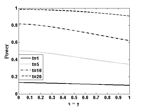
Refer to caption
(a) p=2𝑝2p=2
Refer to caption
(b) p=10𝑝10p=10
Refer to caption
(c) p=50𝑝50p=50
Refer to caption
(d) p=200𝑝200p=200
Figure 1: Asymptotic contiguous power of the simple DPD based test of 𝜷𝜷{\boldsymbol{\beta}} for different values of t=𝚫T𝚺x𝚫𝑡superscript𝚫𝑇subscript𝚺𝑥𝚫t=\boldsymbol{\Delta}^{T}\boldsymbol{\Sigma}_{x}\boldsymbol{\Delta} and p𝑝p, the number of explanatory variables

Next we study the asymptotic power of the proposed test. We derive its asymptotic power under the contiguous alternatives H1,nsubscript𝐻1𝑛H_{1,n} using Corollary 2. The asymptotic distribution of Tγ(𝜷nτ,𝜷0)subscript𝑇𝛾superscriptsubscript𝜷𝑛𝜏subscript𝜷0T_{\gamma}({{\boldsymbol{\beta}}_{n}^{\tau}},{{\boldsymbol{\beta}}_{0}}) under H1,nsubscript𝐻1𝑛H_{1,n} is ζ1γ,τχp,δ2superscriptsubscript𝜁1𝛾𝜏subscriptsuperscript𝜒2𝑝𝛿\zeta_{1}^{\gamma,\tau}\chi^{2}_{p,\delta} with δ=1υτ𝜷𝚫T𝚺x𝚫𝛿1superscriptsubscript𝜐𝜏𝜷superscript𝚫𝑇subscript𝚺𝑥𝚫\delta=\frac{1}{\upsilon_{\tau}^{\boldsymbol{\beta}}}\boldsymbol{\Delta}^{T}\boldsymbol{\Sigma}_{x}\boldsymbol{\Delta}, where υτ𝜷=σ2(1+τ21+2τ)32superscriptsubscript𝜐𝜏𝜷superscript𝜎2superscript1superscript𝜏212𝜏32\upsilon_{\tau}^{{\mathbf{\boldsymbol{\beta}}}}=\sigma^{2}\left(1+\frac{\tau^{2}}{1+2\tau}\right)^{\frac{3}{2}}. Thus its asymptotic contiguous power is Pτ,γ(𝚫,0;α)subscript𝑃𝜏𝛾𝚫0𝛼P_{\tau,\gamma}(\boldsymbol{\Delta},0;\alpha) =P(ζ1γ,τWp,δ>ζ1γ,τχp,α2)absent𝑃superscriptsubscript𝜁1𝛾𝜏subscript𝑊𝑝𝛿superscriptsubscript𝜁1𝛾𝜏subscriptsuperscript𝜒2𝑝𝛼=P\left(\zeta_{1}^{\gamma,\tau}W_{p,\delta}>\zeta_{1}^{\gamma,\tau}\chi^{2}_{p,\alpha}\right) =1Gp,δ(χp,α2),absent1subscript𝐺𝑝𝛿subscriptsuperscript𝜒2𝑝𝛼=1-G_{p,\delta}(\chi^{2}_{p,\alpha}), where Gp,δsubscript𝐺𝑝𝛿G_{p,\delta} is the distribution function of χp,δ2subscriptsuperscript𝜒2𝑝𝛿\chi^{2}_{p,\delta}. Figure 1 shows the asymptotic power over the tuning parameters γ=τ𝛾𝜏\gamma=\tau for different values of 𝚫T𝚺x𝚫(=t, say)\boldsymbol{\Delta}^{T}\boldsymbol{\Sigma}_{x}\boldsymbol{\Delta}~{}(=t,~{}\mbox{ say}); it does not depend on the tuning parameter γ𝛾\gamma. The power depends on the distance (𝚫𝚫\boldsymbol{\Delta}) of the contiguous alternatives from null and the limiting second order moments (𝚺xsubscript𝚺𝑥\boldsymbol{\Sigma}_{x}) of the covariates through t=𝚫T𝚺x𝚫𝑡superscript𝚫𝑇subscript𝚺𝑥𝚫t=\boldsymbol{\Delta}^{T}\boldsymbol{\Sigma}_{x}\boldsymbol{\Delta}; for any fixed τ=γ𝜏𝛾\tau=\gamma it increases as the value of t𝑡t increases. It also depends on the number (p𝑝p) of explanatory variables used. In Figure 1, we show the cases of p𝑝p is 2 and 10 as well as p=50𝑝50p=50 and 200. For fixed values of γ=τ𝛾𝜏\gamma=\tau and 𝚫1T𝚺x𝚫1superscriptsubscript𝚫1𝑇subscript𝚺𝑥subscript𝚫1\boldsymbol{\Delta}_{1}^{T}\boldsymbol{\Sigma}_{x}\boldsymbol{\Delta}_{1}, the power decreases as p𝑝p increases; this is expected as the number of components of 𝜷𝜷{\boldsymbol{\beta}} increases with p𝑝p. The power against any contiguous alternative and any model is seen to decrease slightly with increasing τ𝜏\tau which brings in the non-centrality parameter δ𝛿\delta and hence the asymptotic variance υτ𝜷superscriptsubscript𝜐𝜏𝜷\upsilon_{\tau}^{\boldsymbol{\beta}} of each element of (𝑿T𝑿)1/2𝜷nτsuperscriptsuperscript𝑿𝑇𝑿12superscriptsubscript𝜷𝑛𝜏(\boldsymbol{X}^{T}\boldsymbol{X})^{1/2}\boldsymbol{\beta}_{n}^{\tau}. As υτ𝜷superscriptsubscript𝜐𝜏𝜷\upsilon_{\tau}^{\boldsymbol{\beta}} increases slightly with τ𝜏\tau, the efficiency of the MDPDE and the asymptotic contiguous power of the DPDTS decrease slightly.

We simulated finite-sample situations with different sample sizes n𝑛n and values of t=𝚫T𝚺x𝚫𝑡superscript𝚫𝑇subscript𝚺𝑥𝚫t=\boldsymbol{\Delta}^{T}\boldsymbol{\Sigma}_{x}\boldsymbol{\Delta} and p𝑝p. The convergence of the finite-sample power to the asymptotic value depends on the convergence rate of 1n(𝑿T𝑿)1𝑛superscript𝑿𝑇𝑿\frac{1}{n}(\boldsymbol{X}^{T}\boldsymbol{X}) in Condition (C6); we chose X𝑋X to be a p𝑝p-variate normal distribution with mean 00 and covariance matrix σx2𝑰psuperscriptsubscript𝜎𝑥2subscript𝑰𝑝\sigma_{x}^{2}\boldsymbol{I}_{p} so that (C6) holds with 𝚺x=σx2𝑰psubscript𝚺𝑥superscriptsubscript𝜎𝑥2subscript𝑰𝑝\boldsymbol{\Sigma}_{x}=\sigma_{x}^{2}\boldsymbol{I}_{p}. Results from two such simulations with p=2𝑝2p=2 and σx2=5superscriptsubscript𝜎𝑥25\sigma_{x}^{2}=5 are presented in Figure 2; other cases have similar patterns. Clearly the finite-sample powers are close to the asymptotic power in moderate sample sizes like n=100𝑛100n=100 and the convergence rate is little slower for larger t=𝚫T𝚺x𝚫𝑡superscript𝚫𝑇subscript𝚺𝑥𝚫t=\boldsymbol{\Delta}^{T}\boldsymbol{\Sigma}_{x}\boldsymbol{\Delta}.

Refer to caption
(a) 𝚫T𝚺x𝚫=5superscript𝚫𝑇subscript𝚺𝑥𝚫5\boldsymbol{\Delta}^{T}\boldsymbol{\Sigma}_{x}\boldsymbol{\Delta}=5
Refer to caption
(b) 𝚫T𝚺x𝚫=20superscript𝚫𝑇subscript𝚺𝑥𝚫20\boldsymbol{\Delta}^{T}\boldsymbol{\Sigma}_{x}\boldsymbol{\Delta}=20
Figure 2: Comparison of finite-sample empirical power at different sample sizes n𝑛n with asymptotic contiguous power for the simple DPDTS of 𝜷𝜷{\boldsymbol{\beta}} for p=2𝑝2p=2 and σx2=5superscriptsubscript𝜎𝑥25\sigma_{x}^{2}=5

5.1.2 Robustness Results

As the first order IF of DPDTS Tγ(𝜷nτ,𝜷0)subscript𝑇𝛾superscriptsubscript𝜷𝑛𝜏subscript𝜷0T_{\gamma}({{\boldsymbol{\beta}}_{n}^{\tau}},{{\boldsymbol{\beta}}_{0}}) is zero at any simple null, we measure the stability of the proposed test by the second order IF. For contamination in a single direction (i0thsuperscriptsubscript𝑖0thi_{0}^{\rm th} direction), the second order IF at the null 𝜷=𝜷0𝜷subscript𝜷0{\boldsymbol{\beta}}={\boldsymbol{\beta}}_{0} simplifies to

IFi0(2)(ti0,Tγ,τ(1),𝐅¯𝜽0)𝐼superscriptsubscript𝐹subscript𝑖02subscript𝑡subscript𝑖0superscriptsubscript𝑇𝛾𝜏1subscript¯𝐅subscript𝜽0\displaystyle IF_{i_{0}}^{(2)}(t_{i_{0}},T_{\gamma,\tau}^{(1)},\mathbf{\underline{F}}_{{\boldsymbol{\theta}}_{0}})
=(1+γ)ζγ(1+τ)3n[𝒙i0T(𝑿T𝑿)1𝒙i0](ti0𝒙i0T𝜷0)2eτ(ti0𝒙i0T𝜷0)2σ02.absent1𝛾subscript𝜁𝛾superscript1𝜏3𝑛delimited-[]superscriptsubscript𝒙subscript𝑖0𝑇superscriptsuperscript𝑿𝑇𝑿1subscript𝒙subscript𝑖0superscriptsubscript𝑡subscript𝑖0superscriptsubscript𝒙subscript𝑖0𝑇subscript𝜷02superscript𝑒𝜏superscriptsubscript𝑡subscript𝑖0superscriptsubscript𝒙subscript𝑖0𝑇subscript𝜷02superscriptsubscript𝜎02\displaystyle~{}~{}=(1+\gamma)\zeta_{\gamma}(1+\tau)^{3}n[{\boldsymbol{x}_{i_{0}}}^{T}(\boldsymbol{X}^{T}\boldsymbol{X})^{-1}{\boldsymbol{x}_{i_{0}}}](t_{i_{0}}-{\boldsymbol{x}_{i_{0}}}^{T}{{\mathbf{\boldsymbol{\beta}}_{0}}})^{2}e^{-\frac{\tau(t_{i_{0}}-{\boldsymbol{x}_{i_{0}}}^{T}{{\mathbf{\boldsymbol{\beta}}_{0}}})^{2}}{\sigma_{0}^{2}}}.

As expected, the IF depends on the outliers and the leverage points through (ti0𝒙i0T𝜷0)subscript𝑡subscript𝑖0superscriptsubscript𝒙subscript𝑖0𝑇subscript𝜷0(t_{i_{0}}-{\boldsymbol{x}_{i_{0}}}^{T}{{\mathbf{\boldsymbol{\beta}}_{0}}}) and [𝒙i0T(𝑿T𝑿)1𝒙i0]delimited-[]superscriptsubscript𝒙subscript𝑖0𝑇superscriptsuperscript𝑿𝑇𝑿1subscript𝒙subscript𝑖0[{\boldsymbol{x}_{i_{0}}}^{T}(\boldsymbol{X}^{T}\boldsymbol{X})^{-1}{\boldsymbol{x}_{i_{0}}}]. The LIF and PIF of the proposed DPDTS under contiguous alternatives is presented in Section S2.2 of the Online Supplement.

Both the IF and the PIF are bounded with respect to the contamination point ti0subscript𝑡subscript𝑖0t_{i_{0}} for any τ>0𝜏0\tau>0 implying their stability against contamination. Both are unbounded at ti0subscript𝑡subscript𝑖0t_{i_{0}} for the LRT at γ=τ=0𝛾𝜏0\gamma=\tau=0 indicating its non-robustness. The LIF of this test is identically zero for all τ,γ0𝜏𝛾0\tau,\gamma\geq 0 implying no asymptotic influence of contiguous contamination on its size.

6 Application (II): Generalized Linear Model

In a generalized linear model (GLM), the response variables Yisubscript𝑌𝑖Y_{i} are independent and have an exponential family distribution with density f(yi;θi,ϕ)=exp{yiθib(θi)a(ϕ)+c(yi,ϕ)}𝑓subscript𝑦𝑖subscript𝜃𝑖italic-ϕsubscript𝑦𝑖subscript𝜃𝑖𝑏subscript𝜃𝑖𝑎italic-ϕ𝑐subscript𝑦𝑖italic-ϕf(y_{i};{{\theta}}_{i},\phi)=\exp\left\{\frac{y_{i}{{\theta}}_{i}-b({{\theta}}_{i})}{a(\phi)}+c(y_{i},\phi)\right\}; the canonical parameter θisubscript𝜃𝑖{{\theta}}_{i} depends on the predictor 𝒙isubscript𝒙𝑖{\boldsymbol{x}_{i}} and ϕitalic-ϕ\phi is a nuisance scale parameter. The mean μisubscript𝜇𝑖\mu_{i} of Yisubscript𝑌𝑖Y_{i} satisfies g(μi)=ηi=𝒙iT𝜷,𝑔subscript𝜇𝑖subscript𝜂𝑖superscriptsubscript𝒙𝑖𝑇𝜷g(\mu_{i})=\eta_{i}={\boldsymbol{x}_{i}}^{T}{\boldsymbol{\beta}}, for a monotone differentiable link function g𝑔g and linear predictor ηi=𝒙iT𝜷subscript𝜂𝑖superscriptsubscript𝒙𝑖𝑇𝜷\eta_{i}={\boldsymbol{x}_{i}}^{T}{\boldsymbol{\beta}}.

The GLMs with fixed predictors fit the general I-NH set-up. The properties of the MDPDEs of 𝜽=(𝜷,ϕ)𝜽𝜷italic-ϕ{\boldsymbol{\theta}}=({\boldsymbol{\beta}},\phi) in the GLM were derived in Ghosh and Basu (2016) and are presented in Section S3 of the Online Supplement.

Suppose we have a sample of size n𝑛n from a GLM with parameter 𝜽=(𝜷,ϕ)Θ=p×[0,)𝜽𝜷italic-ϕΘsuperscript𝑝0{\boldsymbol{\theta}}=({\boldsymbol{\beta}},~{}\phi)\in\Theta=\mathbb{R}^{p}\times[0,\infty) and want to test the hypothesis

H0:𝑳T𝜷=𝒍0 against H1:𝑳T𝜷𝒍0,:subscript𝐻0superscript𝑳𝑇𝜷subscript𝒍0 against subscript𝐻1:superscript𝑳𝑇𝜷subscript𝒍0\displaystyle H_{0}:\boldsymbol{L}^{T}{\boldsymbol{\beta}}=\boldsymbol{l}_{0}~{}~{}~{}~{}\mbox{ against }~{}~{}~{}~{}~{}H_{1}:\boldsymbol{L}^{T}{\boldsymbol{\beta}}\neq\boldsymbol{l}_{0},~{}~{} (6.16)

where 𝑳𝑳\boldsymbol{L} is a p×r𝑝𝑟p\times r known matrix with pr𝑝𝑟p\geq r and 𝒍0subscript𝒍0\boldsymbol{l}_{0} is a real r𝑟r-vector. We assume that the nuisance parameter ϕitalic-ϕ\phi is unknown.

The DPD based test statistic (DPDTSC) for testing this problem is

Sγ(𝜽nτ,𝜽~nτ)=2i=1ndγ(fi(.;(𝜷^nτ,ϕ^nτ)),fi(.;(𝜷n~τ,ϕn~τ))),S_{\gamma}({{\boldsymbol{\theta}}_{n}^{\tau}},{\widetilde{{\boldsymbol{\theta}}}_{n}^{\tau}})=2\sum_{i=1}^{n}d_{\gamma}(f_{i}(.;(\widehat{\boldsymbol{\beta}}_{n}^{\tau},\widehat{\phi}_{n}^{\tau})),f_{i}(.;(\widetilde{{\boldsymbol{\beta}}_{n}}^{\tau},\widetilde{\phi_{n}}^{\tau}))),

where 𝜽nτ=(𝜷^nτ,ϕ^nτ)superscriptsubscript𝜽𝑛𝜏superscriptsubscript^𝜷𝑛𝜏superscriptsubscript^italic-ϕ𝑛𝜏{{\boldsymbol{\theta}}_{n}^{\tau}}=(\widehat{\boldsymbol{\beta}}_{n}^{\tau},\widehat{\phi}_{n}^{\tau}) is the unrestricted MDPDE, 𝜽~nτ=(𝜷n~τ,ϕn~τ)superscriptsubscript~𝜽𝑛𝜏superscript~subscript𝜷𝑛𝜏superscript~subscriptitalic-ϕ𝑛𝜏{\widetilde{{\boldsymbol{\theta}}}_{n}^{\tau}}=(\widetilde{{\boldsymbol{\beta}}_{n}}^{\tau},\widetilde{\phi_{n}}^{\tau}) is the restricted MDPDE under H0subscript𝐻0H_{0} corresponding to the tuning parameter τ𝜏\tau.

To derive the asymptotic distribution of the RMDPDE (𝜷n~τ,ϕn~τ)superscript~subscript𝜷𝑛𝜏superscript~subscriptitalic-ϕ𝑛𝜏(\widetilde{{\boldsymbol{\beta}}_{n}}^{\tau},\widetilde{\phi_{n}}^{\tau}) of (𝜷,ϕ)𝜷italic-ϕ({\boldsymbol{\beta}},\phi) from Theorem 5, some simple matrix algebra leads to

𝑷nτ(𝜷,σ)=n[𝚿n,11.21[𝑰p𝑳{𝑳T𝚿n,11.21𝑳}1𝑳T𝚿n,11.21]𝑴11𝑿T𝚪12(τ)𝟏𝚿n,22.11𝚿n,22.11𝟏T𝚪12(τ)𝑿𝑴11𝚿n,22.11],superscriptsubscript𝑷𝑛𝜏𝜷𝜎𝑛matrixsuperscriptsubscript𝚿𝑛11.21delimited-[]subscript𝑰𝑝𝑳superscriptsuperscript𝑳𝑇superscriptsubscript𝚿𝑛11.21𝑳1superscript𝑳𝑇superscriptsubscript𝚿𝑛11.21subscript𝑴11superscript𝑿𝑇superscriptsubscript𝚪12𝜏1superscriptsubscript𝚿𝑛22.11superscriptsubscript𝚿𝑛22.11superscript1𝑇superscriptsubscript𝚪12𝜏𝑿subscript𝑴11superscriptsubscript𝚿𝑛22.11\displaystyle\boldsymbol{P}_{n}^{\tau}({\boldsymbol{\beta}},\sigma)=n~{}\begin{bmatrix}~{}~{}\boldsymbol{\Psi}_{n,11.2}^{-1}\left[\boldsymbol{I}_{p}-\boldsymbol{L}\{\boldsymbol{L}^{T}\boldsymbol{\Psi}_{n,11.2}^{-1}\boldsymbol{L}\}^{-1}\boldsymbol{L}^{T}\boldsymbol{\Psi}_{n,11.2}^{-1}\right]&-\boldsymbol{M}_{11}\boldsymbol{X}^{T}\boldsymbol{\Gamma}_{12}^{(\tau)}\mathbf{1}\boldsymbol{\Psi}_{n,22.1}^{-1}~{}~{}\\ ~{}~{}-\boldsymbol{\Psi}_{n,22.1}^{-1}\mathbf{1}^{T}\boldsymbol{\Gamma}_{12}^{(\tau)}\boldsymbol{X}\boldsymbol{M}_{11}&\boldsymbol{\Psi}_{n,22.1}^{-1}~{}~{}\end{bmatrix},

where, for any i,j=1,2formulae-sequence𝑖𝑗12i,j=1,2, 𝚿n,ii.j=𝑿T𝚪jj(τ)𝑿𝑿T𝚪ij(τ)𝟏(𝟏T𝚪jj(τ)𝟏)1𝟏T𝚪ji(τ)𝑿subscript𝚿formulae-sequence𝑛𝑖𝑖𝑗superscript𝑿𝑇superscriptsubscript𝚪𝑗𝑗𝜏𝑿superscript𝑿𝑇superscriptsubscript𝚪𝑖𝑗𝜏1superscriptsuperscript1𝑇superscriptsubscript𝚪𝑗𝑗𝜏11superscript1𝑇superscriptsubscript𝚪𝑗𝑖𝜏𝑿\boldsymbol{\Psi}_{n,ii.j}=\boldsymbol{X}^{T}\boldsymbol{\Gamma}_{jj}^{(\tau)}\boldsymbol{X}-\boldsymbol{X}^{T}\boldsymbol{\Gamma}_{ij}^{(\tau)}\mathbf{1}(\mathbf{1}^{T}\boldsymbol{\Gamma}_{jj}^{(\tau)}\mathbf{1})^{-1}\mathbf{1}^{T}\boldsymbol{\Gamma}_{ji}^{(\tau)}\boldsymbol{X} with 𝚪ij(τ)superscriptsubscript𝚪𝑖𝑗𝜏\boldsymbol{\Gamma}_{ij}^{(\tau)} defined in Section 4 of the online Supplement, and 𝑴11=(𝑿T𝚪11(τ)𝑿)1subscript𝑴11superscriptsuperscript𝑿𝑇superscriptsubscript𝚪11𝜏𝑿1\boldsymbol{M}_{11}=(\boldsymbol{X}^{T}\boldsymbol{\Gamma}_{11}^{(\tau)}\boldsymbol{X})^{-1}.

Corollary 6.

Suppose the Ghosh-Basu conditions hold with respect to Θ0subscriptΘ0\Theta_{0}. The RMDPDE (𝛃n~,ϕn~)~subscript𝛃𝑛~subscriptitalic-ϕ𝑛(\widetilde{{\boldsymbol{\beta}}_{n}},\widetilde{\phi_{n}}) exists and is consistent for 𝛉0=(𝛃g,ϕg)subscript𝛉0superscript𝛃𝑔superscriptitalic-ϕ𝑔{\boldsymbol{\theta}}_{0}=({\boldsymbol{\beta}}^{g},\phi^{g}), true parameter value under Θ0subscriptΘ0\Theta_{0}. The asymptotic distribution of 𝛀n12𝐏n[n((𝛃n~,ϕn~)(𝛃g~,ϕg~))]superscriptsubscript𝛀𝑛12subscript𝐏𝑛delimited-[]𝑛~subscript𝛃𝑛~subscriptitalic-ϕ𝑛~superscript𝛃𝑔~superscriptitalic-ϕ𝑔\boldsymbol{\Omega}_{n}^{-\frac{1}{2}}\boldsymbol{P}_{n}\left[\sqrt{n}\left((\widetilde{{\boldsymbol{\beta}}_{n}},\widetilde{\phi_{n}})-(\widetilde{{\boldsymbol{\beta}}^{g}},\widetilde{\phi^{g}})\right)\right] is (p+1)𝑝1(p+1)-dimensional normal with mean 𝟎0\boldsymbol{0} and variance 𝐈p+1subscript𝐈𝑝1\boldsymbol{I}_{p+1}, where 𝐏n=𝐏nτ(𝛃g~,ϕg~)subscript𝐏𝑛superscriptsubscript𝐏𝑛𝜏~superscript𝛃𝑔~superscriptitalic-ϕ𝑔\boldsymbol{P}_{n}=\boldsymbol{P}_{n}^{\tau}(\widetilde{{\boldsymbol{\beta}}^{g}},\widetilde{\phi^{g}}) and 𝛀n=𝛀nτ(𝛃g~,ϕg~)subscript𝛀𝑛superscriptsubscript𝛀𝑛𝜏~superscript𝛃𝑔~superscriptitalic-ϕ𝑔\boldsymbol{\Omega}_{n}=\boldsymbol{\Omega}_{n}^{\tau}(\widetilde{{\boldsymbol{\beta}}^{g}},\widetilde{\phi^{g}}), with 𝛀n(𝛃,ϕ)subscript𝛀𝑛𝛃italic-ϕ\boldsymbol{\Omega}_{n}({\boldsymbol{\beta}},\phi) defined in Section S3 of the Online Supplement.

As in the unrestricted case, the restricted MDPDE of 𝜷𝜷{\boldsymbol{\beta}} and ϕitalic-ϕ\phi may not be asymptotically independent. They are independent if γ12i1+2τ=0,γ1i1+τγ2i1+τ=0,iformulae-sequencesuperscriptsubscript𝛾12𝑖12𝜏0superscriptsubscript𝛾1𝑖1𝜏superscriptsubscript𝛾2𝑖1𝜏0for-all𝑖\gamma_{12i}^{1+2\tau}=0,\gamma_{1i}^{1+\tau}\gamma_{2i}^{1+\tau}=0,~{}\forall i.

To derive asymptotic distribution of the DPDTSC, we assume fixed covariates 𝒙isubscript𝒙𝑖{\boldsymbol{x}_{i}}’s for which the matrices 𝚿nτ(𝜽~g)superscriptsubscript𝚿𝑛𝜏superscript~𝜽𝑔\boldsymbol{\Psi}_{n}^{\tau}(\widetilde{{\boldsymbol{\theta}}}^{g}) and 𝛀nτ(𝜽~g)superscriptsubscript𝛀𝑛𝜏superscript~𝜽𝑔\boldsymbol{\Omega}_{n}^{\tau}(\widetilde{{\boldsymbol{\theta}}}^{g}), defined in Section S3 of the Online Supplement, converge element-wise as n𝑛n\rightarrow\infty to some (p+1)×(p+1)𝑝1𝑝1(p+1)\times(p+1) invertible matrices 𝑱τsubscript𝑱𝜏{\boldsymbol{J}_{\tau}} and 𝑽τsubscript𝑽𝜏{\boldsymbol{V}_{\tau}}, respectively. Consider the partitions

𝑱τ(𝜷,σ)=[𝑱11,τ𝑱12,τ𝑱12,τT𝑱22,τ], and 𝑽τ(𝜷,σ)=[𝑽11,τ𝑽12,τ𝑽12,τT𝑽22,τ],formulae-sequencesubscript𝑱𝜏𝜷𝜎matrixsubscript𝑱11𝜏subscript𝑱12𝜏superscriptsubscript𝑱12𝜏𝑇subscript𝑱22𝜏 and subscript𝑽𝜏𝜷𝜎matrixsubscript𝑽11𝜏subscript𝑽12𝜏superscriptsubscript𝑽12𝜏𝑇subscript𝑽22𝜏{\boldsymbol{J}_{\tau}}({\boldsymbol{\beta}},\sigma)=\begin{bmatrix}~{}~{}\boldsymbol{J}_{11,\tau}&\boldsymbol{J}_{12,\tau}~{}\\ ~{}~{}\boldsymbol{J}_{12,\tau}^{T}&\boldsymbol{J}_{22,\tau}~{}\end{bmatrix},~{}~{}~{}~{}~{}\mbox{ and }~{}~{}~{}~{}~{}{\boldsymbol{V}_{\tau}}({\boldsymbol{\beta}},\sigma)=\begin{bmatrix}~{}~{}\boldsymbol{V}_{11,\tau}&\boldsymbol{V}_{12,\tau}~{}\\ ~{}~{}\boldsymbol{V}_{12,\tau}^{T}&\boldsymbol{V}_{22,\tau}~{}\end{bmatrix},

where 𝑱11,τsubscript𝑱11𝜏\boldsymbol{J}_{11,\tau} and 𝑽11,τsubscript𝑽11𝜏\boldsymbol{V}_{11,\tau} are of order p×p𝑝𝑝p\times p. We suppress τ𝜏\tau in above notation whenever it is clear from the context. Then, the asymptotic null distribution of the DPDTSC Sγ(𝜽nτ,𝜽~nτ)subscript𝑆𝛾superscriptsubscript𝜽𝑛𝜏superscriptsubscript~𝜽𝑛𝜏S_{\gamma}({{\boldsymbol{\theta}}_{n}^{\tau}},{\widetilde{{\boldsymbol{\theta}}}_{n}^{\tau}}) follows directly from Theorem 6 provided the Ghosh-Basu conditions hold for the model under H0subscript𝐻0H_{0}.

Corollary 7.

For the GLM set-up, assume that its density satisfies the Lehmann and Ghosh-Basu conditions under Θ0subscriptΘ0\Theta_{0}. Then the asymptotic null distribution of the DPDTSC Sγ(𝛉nτ,𝛉~nτ)subscript𝑆𝛾superscriptsubscript𝛉𝑛𝜏superscriptsubscript~𝛉𝑛𝜏S_{\gamma}({{\boldsymbol{\theta}}_{n}^{\tau}},{\widetilde{{\boldsymbol{\theta}}}_{n}^{\tau}}) is the same as that of i=1rζiγ,τ(𝛉0)Zi2,superscriptsubscript𝑖1𝑟superscriptsubscript𝜁𝑖𝛾𝜏subscript𝛉0superscriptsubscript𝑍𝑖2\sum_{i=1}^{r}~{}\zeta_{i}^{\gamma,\tau}({\boldsymbol{\theta}}_{0})Z_{i}^{2}, where Z1,,Zrsubscript𝑍1subscript𝑍𝑟Z_{1},\cdots,Z_{r} are independent standard normal variables, and ζ1γ,τ(𝛉0)superscriptsubscript𝜁1𝛾𝜏subscript𝛉0\zeta_{1}^{\gamma,\tau}({\boldsymbol{\theta}}_{0}), ,ζrγ,τ(𝛉0)superscriptsubscript𝜁𝑟𝛾𝜏subscript𝛉0\cdots,\zeta_{r}^{\gamma,\tau}({\boldsymbol{\theta}}_{0}) are r𝑟r nonzero eigenvalues of the matrix

𝑬=(1+γ)𝑱11,γ𝑱11.21𝑳𝑵11𝑳T𝑱11.21𝑽11𝑱11.21𝑳𝑵11𝑳T𝑱11.21,𝑬1𝛾subscript𝑱11𝛾superscriptsubscript𝑱11.21𝑳subscript𝑵11superscript𝑳𝑇superscriptsubscript𝑱11.21subscript𝑽11superscriptsubscript𝑱11.21𝑳subscript𝑵11superscript𝑳𝑇superscriptsubscript𝑱11.21\boldsymbol{E}=(1+\gamma)\boldsymbol{J}_{11,\gamma}\boldsymbol{J}_{11.2}^{-1}\boldsymbol{L}\boldsymbol{N}_{11}\boldsymbol{L}^{T}\boldsymbol{J}_{11.2}^{-1}\boldsymbol{V}_{11}\boldsymbol{J}_{11.2}^{-1}\boldsymbol{L}\boldsymbol{N}_{11}\boldsymbol{L}^{T}\boldsymbol{J}_{11.2}^{-1},

where 𝐉ii.j=𝐉ii,τ𝐉ij,τ𝐉jj,τ1𝐉ji,τTsubscript𝐉formulae-sequence𝑖𝑖𝑗subscript𝐉𝑖𝑖𝜏subscript𝐉𝑖𝑗𝜏superscriptsubscript𝐉𝑗𝑗𝜏1superscriptsubscript𝐉𝑗𝑖𝜏𝑇\boldsymbol{J}_{ii.j}=\boldsymbol{J}_{ii,\tau}-\boldsymbol{J}_{ij,\tau}\boldsymbol{J}_{jj,\tau}^{-1}\boldsymbol{J}_{ji,\tau}^{T} for i,j=1,2;ijformulae-sequence𝑖𝑗12𝑖𝑗i,j=1,2;i\neq j and 𝐍11=(𝐋T𝐉11.21𝐋)1subscript𝐍11superscriptsuperscript𝐋𝑇superscriptsubscript𝐉11.21𝐋1\boldsymbol{N}_{11}=(\boldsymbol{L}^{T}\boldsymbol{J}_{11.2}^{-1}\boldsymbol{L})^{-1}.

This result can be used to obtain the critical values of the proposed DPD based test. The other asymptotic results regarding power and robustness of the test can be derived by direct application of the general theory of Section 4. For instance, the second order IF of the test statistics at the null hypothesis, when there is contamination in only one fixed direction-i0subscript𝑖0i_{0}, is

IFi0(2)(ti0,Sγ,τ(1),𝐅¯𝜽0)=n(1+γ)𝑾T𝚿nγ𝑾,𝐼superscriptsubscript𝐹subscript𝑖02subscript𝑡subscript𝑖0superscriptsubscript𝑆𝛾𝜏1subscript¯𝐅subscript𝜽0𝑛1𝛾superscript𝑾𝑇superscriptsubscript𝚿𝑛𝛾𝑾\displaystyle IF_{i_{0}}^{(2)}(t_{i_{0}},S_{\gamma,\tau}^{(1)},\underline{\mathbf{F}}_{{\boldsymbol{\theta}}_{0}})=n(1+\gamma)\cdot\boldsymbol{W}^{T}\boldsymbol{\Psi}_{n}^{\gamma}\boldsymbol{W}, (6.17)
where 𝑾=𝚿n11n([fi0(ti0;(𝜷,ϕ))τK1i0(ti0;(𝜷,ϕ))γ1i0]𝒙ifi0(ti0;(𝜷,ϕ))τK2i0(ti0;(𝜷,ϕ))γ2i0)𝑾superscriptsubscript𝚿𝑛11𝑛delimited-[]subscript𝑓subscript𝑖0superscriptsubscript𝑡subscript𝑖0𝜷italic-ϕ𝜏subscript𝐾1subscript𝑖0subscript𝑡subscript𝑖0𝜷italic-ϕsubscript𝛾1subscript𝑖0subscript𝒙𝑖subscript𝑓subscript𝑖0superscriptsubscript𝑡subscript𝑖0𝜷italic-ϕ𝜏subscript𝐾2subscript𝑖0subscript𝑡subscript𝑖0𝜷italic-ϕsubscript𝛾2subscript𝑖0\displaystyle\boldsymbol{W}=\boldsymbol{\Psi}_{n}^{-1}\frac{1}{n}\left(\begin{array}[]{c}\left[f_{i_{0}}(t_{i_{0}};({\boldsymbol{\beta}},\phi))^{\tau}K_{1i_{0}}(t_{i_{0}};({\boldsymbol{\beta}},\phi))-\gamma_{1i_{0}}\right]{\boldsymbol{x}_{i}}\\ f_{i_{0}}(t_{i_{0}};({\boldsymbol{\beta}},\phi))^{\tau}K_{2i_{0}}(t_{i_{0}};({\boldsymbol{\beta}},\phi))-\gamma_{2i_{0}}\end{array}\right) (6.23)
𝑸(𝜽0)1𝚿n(0)(𝜽0)T1n(fi0(ti0;𝜽0)τ𝒖1i0(0)(ti0;𝜽0)𝜸1i0(0)fi0(ti0;𝜽0)τ𝒖2i0(0)(ti0;𝜽0)𝜸2i0(0)),𝑸superscriptsubscript𝜽01superscriptsubscript𝚿𝑛0superscriptsubscript𝜽0𝑇1𝑛subscript𝑓subscript𝑖0superscriptsubscript𝑡subscript𝑖0subscript𝜽0𝜏superscriptsubscript𝒖1subscript𝑖00subscript𝑡subscript𝑖0subscript𝜽0superscriptsubscript𝜸1subscript𝑖00subscript𝑓subscript𝑖0superscriptsubscript𝑡subscript𝑖0subscript𝜽0𝜏superscriptsubscript𝒖2subscript𝑖00subscript𝑡subscript𝑖0subscript𝜽0superscriptsubscript𝜸2subscript𝑖00\displaystyle~{}~{}~{}-\boldsymbol{Q}({\boldsymbol{\theta}}_{0})^{-1}\boldsymbol{\Psi}_{n}^{(0)}({{\boldsymbol{\theta}}_{0}})^{T}\frac{1}{n}\left(\begin{array}[]{c}f_{i_{0}}(t_{i_{0}};{\boldsymbol{\theta}}_{0})^{\tau}\boldsymbol{u}_{1i_{0}}^{(0)}(t_{i_{0}};{\boldsymbol{\theta}}_{0})-\boldsymbol{\gamma}_{1i_{0}}^{(0)}\\ f_{i_{0}}(t_{i_{0}};{\boldsymbol{\theta}}_{0})^{\tau}\boldsymbol{u}_{2i_{0}}^{(0)}(t_{i_{0}};{\boldsymbol{\theta}}_{0})-\boldsymbol{\gamma}_{2i_{0}}^{(0)}\end{array}\right),~{}~{}~{}~{}

with Kji0(ti0;(𝜷,ϕ))subscript𝐾𝑗subscript𝑖0subscript𝑡subscript𝑖0𝜷italic-ϕK_{ji_{0}}(t_{i_{0}};({\boldsymbol{\beta}},\phi)) as defined in Section S3 of the Online Supplement for j=1,2𝑗12j=1,2, 𝒖1i(0)(yi;(𝜷,ϕ))superscriptsubscript𝒖1𝑖0subscript𝑦𝑖𝜷italic-ϕ\boldsymbol{u}_{1i}^{(0)}(y_{i};({\boldsymbol{\beta}},\phi)) and 𝒖2i(0)(yi;(𝜷,ϕ))superscriptsubscript𝒖2𝑖0subscript𝑦𝑖𝜷italic-ϕ\boldsymbol{u}_{2i}^{(0)}(y_{i};({\boldsymbol{\beta}},\phi)) denoting the restricted derivative of logfi(yi;(𝜷,ϕ))subscript𝑓𝑖subscript𝑦𝑖𝜷italic-ϕ\log~{}f_{i}(y_{i};({\boldsymbol{\beta}},\phi)) with respect to 𝜷𝜷{\boldsymbol{\beta}} and ϕitalic-ϕ\phi under H0subscript𝐻0H_{0}, and 𝚿n(0)superscriptsubscript𝚿𝑛0\boldsymbol{\Psi}_{n}^{(0)} being the matrix 𝚿nsubscript𝚿𝑛\boldsymbol{\Psi}_{n} constructed using (𝒖1i(0),𝒖1i(0))superscriptsubscript𝒖1𝑖0superscriptsubscript𝒖1𝑖0(\boldsymbol{u}_{1i}^{(0)},\boldsymbol{u}_{1i}^{(0)}) in place of 𝒖i=(𝒖1i,𝒖2i)Tsubscript𝒖𝑖superscriptsubscript𝒖1𝑖subscript𝒖2𝑖𝑇{\boldsymbol{u}_{i}}=(\boldsymbol{u}_{1i},~{}\boldsymbol{u}_{2i})^{T}.

Example 6.1. Consider testing the first r𝑟r components (rp𝑟𝑝r\leq p) of the regression coefficient 𝜷𝜷{\boldsymbol{\beta}} at a pre-fixed value 𝜷0(1)superscriptsubscript𝜷01{\boldsymbol{\beta}}_{0}^{(1)}, the null hypothesis given by (6.16) with 𝑳=[𝑰r𝑶(pr)×r]𝑳matrixsubscript𝑰𝑟subscript𝑶𝑝𝑟𝑟\boldsymbol{L}=\begin{bmatrix}~{}~{}\boldsymbol{I}_{r}~{}\\ ~{}~{}\boldsymbol{O}_{(p-r)\times r}~{}\end{bmatrix}.

We partition the relevant vectors and matrices as 𝜷=(𝜷0(1),𝜷0(2))𝜷superscriptsubscript𝜷01superscriptsubscript𝜷02{\boldsymbol{\beta}}=({\boldsymbol{\beta}}_{0}^{(1)},~{}{\boldsymbol{\beta}}_{0}^{(2)}), 𝒙i=(𝒙i(1),𝒙i(2))subscript𝒙𝑖superscriptsubscript𝒙𝑖1superscriptsubscript𝒙𝑖2{\boldsymbol{x}_{i}}=({\boldsymbol{x}_{i}}^{(1)},~{}{\boldsymbol{x}_{i}}^{(2)}) and 𝑿=[𝑿1𝑿2]𝑿delimited-[]subscript𝑿1subscript𝑿2\boldsymbol{X}=[\boldsymbol{X}_{1}~{}\boldsymbol{X}_{2}], where 𝜷0(1)superscriptsubscript𝜷01{\boldsymbol{\beta}}_{0}^{(1)} and 𝒙i(1)superscriptsubscript𝒙𝑖1{\boldsymbol{x}_{i}}^{(1)} are r𝑟r-vectors and 𝑿1subscript𝑿1\boldsymbol{X}_{1} is the n×r𝑛𝑟n\times r matrix consisting of the first r𝑟r columns of 𝑿𝑿\boldsymbol{X}. Let

𝑱11=[𝑱1111𝑱1112(𝑱1112)T𝑱1122],𝑽11=[𝑽1111𝑽1112(𝑽1112)T𝑽1122],𝑱11.21=[𝑱11.211𝑱11.212(𝑱11.212)T𝑱11.222],formulae-sequencesubscript𝑱11matrixsuperscriptsubscript𝑱1111superscriptsubscript𝑱1112superscriptsuperscriptsubscript𝑱1112𝑇superscriptsubscript𝑱1122formulae-sequencesubscript𝑽11matrixsuperscriptsubscript𝑽1111superscriptsubscript𝑽1112superscriptsuperscriptsubscript𝑽1112𝑇superscriptsubscript𝑽1122superscriptsubscript𝑱11.21matrixsuperscriptsubscript𝑱11.211superscriptsubscript𝑱11.212superscriptsuperscriptsubscript𝑱11.212𝑇superscriptsubscript𝑱11.222\boldsymbol{J}_{11}=\begin{bmatrix}~{}~{}\boldsymbol{J}_{11}^{11}&\boldsymbol{J}_{11}^{12}~{}\\ ~{}~{}(\boldsymbol{J}_{11}^{12})^{T}&\boldsymbol{J}_{11}^{22}~{}\end{bmatrix},~{}\boldsymbol{V}_{11}=\begin{bmatrix}~{}~{}\boldsymbol{V}_{11}^{11}&\boldsymbol{V}_{11}^{12}~{}\\ ~{}~{}(\boldsymbol{V}_{11}^{12})^{T}&\boldsymbol{V}_{11}^{22}~{}\end{bmatrix},~{}\boldsymbol{J}_{11.2}^{-1}=\begin{bmatrix}~{}~{}\boldsymbol{J}_{11.2}^{-11}&\boldsymbol{J}_{11.2}^{-12}~{}\\ ~{}~{}(\boldsymbol{J}_{11.2}^{-12})^{T}&\boldsymbol{J}_{11.2}^{-22}~{}\end{bmatrix},

where the first block of each partitioned matrix is of order r×r𝑟𝑟r\times r.

Here the asymptotic distribution of the DPD-based test statistics Sγ(𝜽nτ,𝜽~nτ)subscript𝑆𝛾superscriptsubscript𝜽𝑛𝜏superscriptsubscript~𝜽𝑛𝜏S_{\gamma}({{\boldsymbol{\theta}}_{n}^{\tau}},{\widetilde{{\boldsymbol{\theta}}}_{n}^{\tau}}) under the null is that of i=1rζiγ,τ(𝜽0)Zi2,superscriptsubscript𝑖1𝑟superscriptsubscript𝜁𝑖𝛾𝜏subscript𝜽0superscriptsubscript𝑍𝑖2\sum_{i=1}^{r}~{}\zeta_{i}^{\gamma,\tau}({\boldsymbol{\theta}}_{0})Z_{i}^{2}, where Z1,,Zrsubscript𝑍1subscript𝑍𝑟Z_{1},\cdots,Z_{r} are independent standard normal variables, and ζ1γ,τ(𝜽0),,ζrγ,τ(𝜽0)superscriptsubscript𝜁1𝛾𝜏subscript𝜽0superscriptsubscript𝜁𝑟𝛾𝜏subscript𝜽0\zeta_{1}^{\gamma,\tau}({\boldsymbol{\theta}}_{0}),\cdots,\zeta_{r}^{\gamma,\tau}({\boldsymbol{\theta}}_{0}) are r𝑟r nonzero eigenvalues of the matrix (1+γ)𝑱11,γ11𝑱11.211𝑽1111𝑱11.2111𝛾superscriptsubscript𝑱11𝛾11superscriptsubscript𝑱11.211superscriptsubscript𝑽1111superscriptsubscript𝑱11.211(1+\gamma)\boldsymbol{J}_{11,\gamma}^{11}\boldsymbol{J}_{11.2}^{-11}\boldsymbol{V}_{11}^{11}\boldsymbol{J}_{11.2}^{-11}. We have

𝑾𝑾\displaystyle\boldsymbol{W} =\displaystyle= 𝚿n11n(𝟎r[fi0(ti0;(𝜷,ϕ))τK1i0(ti0;(𝜷,ϕ))γ1i0]𝒙i(2)fi0(ti0;(𝜷,ϕ))τK2i0(ti0;(𝜷,ϕ))γ2i0).superscriptsubscript𝚿𝑛11𝑛subscript0𝑟delimited-[]subscript𝑓subscript𝑖0superscriptsubscript𝑡subscript𝑖0𝜷italic-ϕ𝜏subscript𝐾1subscript𝑖0subscript𝑡subscript𝑖0𝜷italic-ϕsubscript𝛾1subscript𝑖0superscriptsubscript𝒙𝑖2subscript𝑓subscript𝑖0superscriptsubscript𝑡subscript𝑖0𝜷italic-ϕ𝜏subscript𝐾2subscript𝑖0subscript𝑡subscript𝑖0𝜷italic-ϕsubscript𝛾2subscript𝑖0\displaystyle\boldsymbol{\Psi}_{n}^{-1}\frac{1}{n}\left(\begin{array}[]{c}\boldsymbol{0}_{r}\\ \left[f_{i_{0}}(t_{i_{0}};({\boldsymbol{\beta}},\phi))^{\tau}K_{1i_{0}}(t_{i_{0}};({\boldsymbol{\beta}},\phi))-\gamma_{1i_{0}}\right]{\boldsymbol{x}_{i}}^{(2)}\\ f_{i_{0}}(t_{i_{0}};({\boldsymbol{\beta}},\phi))^{\tau}K_{2i_{0}}(t_{i_{0}};({\boldsymbol{\beta}},\phi))-\gamma_{2i_{0}}\end{array}\right). (6.27)

The second order IF follows from (6.17) with this form of 𝑾𝑾\boldsymbol{W}. As expected, there is no influence of contamination on the first r𝑟r components of the RMDPDE. ∎

7 Numerical Illustration: A Data Example

We consider the multiple regression model using the “Salinity data” (Rousseeuw and Leroy (1987, Chapter 2)). These data were discussed in Ruppert and Carroll (1980), Rousseeuw and Leroy (1987), and Ghosh and Basu (2013). Our analysis shows, except for two potential outliers, that the data is well modeled by a multiple linear regression model, taking salinity as the response variable and the covariates as salinity in two weeks lag (x1subscript𝑥1x_{1}), the number of biweekly periods elapsed since the beginning of spring (x2subscript𝑥2x_{2}), and the volume of river discharge into the sound (x3subscript𝑥3x_{3}). Cases 5 and 16 are outlying observations that correspond to periods of very heavy discharge.

The maximum likelihood estimate of the regression coefficient 𝜷=(β0,β1,β2,β3)T𝜷superscriptsubscript𝛽0subscript𝛽1subscript𝛽2subscript𝛽3𝑇{\boldsymbol{\beta}}=(\beta_{0},\beta_{1},\beta_{2},\beta_{3})^{T} and the error standard deviation σ𝜎\sigma for the full data are (9.6,0.8,0.03,0.3)Tsuperscript9.60.80.030.3𝑇(9.6,0.8,-0.03,-0.3)^{T} and 1.231.231.23. After deleting the outlying observations these estimates are (23.39,0.70,0.25,0.84)Tsuperscript23.390.700.250.84𝑇(23.39,0.70,-0.25,-0.84)^{T} and 0.910.910.91, respectively, indicating the dramatic effect of outliers. Ghosh and Basu (2013) showed that the MDPDE with τ0.25𝜏0.25\tau\geq 0.25 can successfully generate robust estimators even under presence of the two outlying observations. In particular, the MDPDEs at τ=0.5𝜏0.5\tau=0.5 and τ=1𝜏1\tau=1 are, respectively, 𝜷^=(18.4,0.72,0.2,0.63)T^𝜷superscript18.40.720.20.63𝑇\widehat{\boldsymbol{\beta}}=(18.4,0.72,-0.2,-0.63)^{T}, σ^=0.87^𝜎0.87\widehat{\sigma}=0.87, and 𝜷^=(19.19,0.71,0.18,0.66)T^𝜷superscript19.190.710.180.66𝑇\widehat{\boldsymbol{\beta}}=(19.19,0.71,-0.18,-0.66)^{T}, σ^=0.87^𝜎0.87\widehat{\sigma}=0.87. These estimates are quite close to the outlier deleted MLE.

We applied the proposed DPD-based test using the full and outlier deleted data. We tested such hypotheses on 𝜷𝜷{\boldsymbol{\beta}} as H0:𝜷=(19.19,0.71,0.18,0.66)T:subscript𝐻0𝜷superscript19.190.710.180.66𝑇H_{0}:{\boldsymbol{\beta}}=(19.19,~{}0.71,~{}-0.18,~{}-0.66)^{T}, H0:𝜷=(18.4,0.72,0.2,0.63)T:subscript𝐻0𝜷superscript18.40.720.20.63𝑇H_{0}:{\boldsymbol{\beta}}=(18.4,0.72,-0.2,-0.63)^{T}, and H0:𝜷=(9.6,0.8,0.03,0.3)T:subscript𝐻0𝜷superscript9.60.80.030.3𝑇H_{0}:{\boldsymbol{\beta}}=(9.6,0.8,-0.03,-0.3)^{T}. They were chosen at the estimated values for two robust estimators, MDPDE at τ=1𝜏1\tau=1 and 0.50.50.5, and the non-robust MLE, respectively. Therefore, a robust test should accept the first two hypotheses while rejecting the third. We considered both simple and composite tests by assuming σ𝜎\sigma to be known and unknown. For the known σ𝜎\sigma case, we assumed two distinct values of σ𝜎\sigma: 1.231.231.23 (a non-robust estimate, MLE) and 0.710.710.71 (a robust estimate, MDPDE at τ=1𝜏1\tau=1). The p-values of the proposed DPD based tests for these cases are presented in Figure 3.
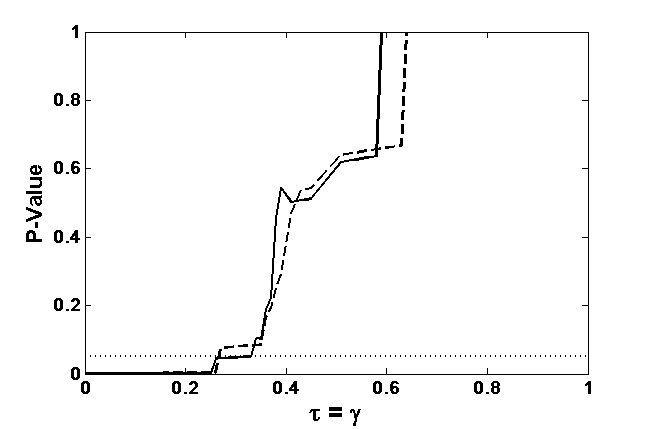
Refer to caption
(a) H0:𝜷:subscript𝐻0𝜷H_{0}:{\boldsymbol{\beta}} = (19.19, 0.71, 0.180.18-0.18, 0.660.66-0.66) (σ=1.23𝜎1.23\sigma=1.23 known)
Refer to caption
(b) H0:𝜷:subscript𝐻0𝜷H_{0}:{\boldsymbol{\beta}} = (19.19, 0.71, 0.180.18-0.18, 0.660.66-0.66) (σ=0.71𝜎0.71\sigma=0.71 known)
Refer to caption
(c) H0:𝜷:subscript𝐻0𝜷H_{0}:{\boldsymbol{\beta}} = (19.19, 0.71, 0.180.18-0.18, 0.660.66-0.66) (σ𝜎\sigma unknown)
Refer to caption
(d) H0:𝜷:subscript𝐻0𝜷H_{0}:{\boldsymbol{\beta}} = (18.4, 0.72, 0.20.2-0.2, 0.630.63-0.63) (σ=1.23𝜎1.23\sigma=1.23 known)
Refer to caption
(e) H0:𝜷:subscript𝐻0𝜷H_{0}:{\boldsymbol{\beta}} = (18.4, 0.72, 0.20.2-0.2, 0.630.63-0.63) (σ=0.71𝜎0.71\sigma=0.71 known)
Refer to caption
(f) H0:𝜷:subscript𝐻0𝜷H_{0}:{\boldsymbol{\beta}} = (18.4, 0.72, 0.20.2-0.2, 0.630.63-0.63) (σ𝜎\sigma unknown)
Refer to caption
(g) H0:𝜷:subscript𝐻0𝜷H_{0}:{\boldsymbol{\beta}} = (9.6, 0.8, 0.030.03-0.03, 0.30.3-0.3) (σ=1.23𝜎1.23\sigma=1.23 known)
Refer to caption
(h) H0:𝜷:subscript𝐻0𝜷H_{0}:{\boldsymbol{\beta}} = (9.6, 0.8, 0.030.03-0.03, 0.30.3-0.3) (σ=0.71𝜎0.71\sigma=0.71 known)
Refer to caption
(i) H0:𝜷:subscript𝐻0𝜷H_{0}:{\boldsymbol{\beta}} = (9.6, 0.8, 0.030.03-0.03, 0.30.3-0.3) (σ𝜎\sigma unknown)
Figure 3: The p-values of the DPD-based tests for different H0subscript𝐻0H_{0}, with known and unknown σ2superscript𝜎2\sigma^{2}, for the Salinity data (Solid line - full data; dashed line - outlier deleted data)

When σ𝜎\sigma is unknown, the DPD-based tests with τ=γ0.2𝜏𝛾0.2\tau=\gamma\geq 0.2 give robust results by failing to reject the first two hypotheses (Figures 3c, 3f) and by rejecting the third one (Figure 3i) under full data. The performances of the LRT at τ=γ=0𝜏𝛾0\tau=\gamma=0 is clearly non-robust under full data. When σ𝜎\sigma is robustly specified, under full data the DPD-based tests still fail to reject the first two hypotheses at larger τ=γ0.5𝜏𝛾0.5\tau=\gamma\geq 0.5 but the LRT rejects them (Figures 3b, 3e). All DPD-based tests, including the LRT, successfully reject the third hypothesis under full data for correctly specified robust σ𝜎\sigma (Figure 3h). When σ𝜎\sigma is incorrectly specified, the DPD-based tests at τ=γ0.5𝜏𝛾0.5\tau=\gamma\geq 0.5 still lead to robust inference while the LRT provides incorrect inference for the first two hypotheses (Figures 3a, 3d); the third hypothesis gets accepted by the DPD-based tests at larger τ=γ𝜏𝛾\tau=\gamma due to the incorrect specification of σ𝜎\sigma (Figure 3g).

8 Conclusions

In this paper we have presented a general framework based on density power divergence for performing robust tests of hypothesis in the independent but non-homogeneous case. We have established the wide scope of the test, and numerically demonstrated its applicability to the linear regression problem. Due to the generality of the method and theoretical indicators it is expected that it will be a powerful tool for the practitioner, although further numerical studies would be helpful to explore the performance of these tests in specific situations.

Among possible extensions, we hope to study the multisample problem. Another extension would be to the case of heteroscedastic models. Finally, the choice of tuning parameters requires a thorough study.

Supplementary Material

The Online Supplement to this paper contains the details of S1. required assumptions; S2. MDPDE under the linear regression model with fixed design along with some additional results for testing; S3. MDPDE under the GLM with fixed design; S4. proofs; S5. simulations under linear regression models; S6. two more data applications from linear and Poisson regression models; and S7. comments on the choice of tuning parameters.

Acknowledgment: The authors thank the referees, the Editor and an associate editor for their constructive comments and suggestions.

References

  • Basu et al. (1998) Basu, A., Harris, I. R., Hjort, N. L., and Jones, M. C. (1998). Robust and efficient estimation by minimising a density power divergence. Biometrika 85, 549–559.
  • Basu et al. (2013a) Basu, A., Mandal, A., Martin, N., and Pardo, L. (2013a). Testing statistical hypotheses based on the density power divergence. Ann. Inst. Statist. Math. 65, 319–348.
  • Basu et al. (2013b) Basu, A., Mandal, A., Martin, N., and Pardo, L. (2013b). Density Power Divergence Tests for Composite Null Hypotheses. ArXiv pre-print, arXiv:1403.0330 [stat.ME].
  • Cantoni and Ronchetti (2001) Cantoni, E., and Ronchetti, E. (2001). Bounded Influence for Generalized Linear Models. J. Amer. Statist. Assoc. 96, 1022–1030.
  • Ghosh (2015) Ghosh, A. (2015). Influence Function of the Restricted Minimum Divergence Estimators : A General Form. Electron. J. Stat. 9, 1017–1040.
  • Ghosh (2017) Ghosh, A. (2017). Divergence based Robust Estimation of Tail Index with Exponential Regression Model. Stat. Methods Appl. 26(2), 181–213.
  • Ghosh and Basu (2013) Ghosh, A., and Basu, A. (2013). Robust Estimation for Independent Non-Homogeneous Observations using Density Power Divergence with Applications to Linear Regression. Electron. J. Stat. 7, 2420–2456.
  • Ghosh and Basu (2016) Ghosh, A., and Basu, A. (2016). Robust Estimation in Generalised Linear Models : The Density Power Divergence Approach. TEST 25(2), 269–290.
  • Hampel et al. (1986) Hampel, F. R., Ronchetti, E., Rousseeuw, P. J., and Stahel, W. (1986). Robust Statistics: The Approach Based on Influence Functions. John Wiley & Sons, New York.
  • Heritier and Ronchetti (1994) Heritier, S., and Ronchetti, E. (1994). Robust bounded-influence tests in general parametric models. J. Amer. Statist. Assoc. 89, 897–904.
  • Hosseinian (2009) Hosseinian, S. (2009). Robust inference for generalized linear models: binary and Poisson regression. Ph. D. thesis, Ecole Polytechnique Federal de Lausanne.
  • Huber (1983) Huber, P. J. (1983). Minimax aspects of bounded-influence regression (with discussion). J. Amer. Statist. Assoc. 78, 66–80.
  • Kotz et al. (1967a) Kotz, S., Johnson, N. L., and Boyd, D. W. (1967a). Series representations of distributions of quadratic forms in normal variables. I. Ann. Math. Statist. 38, 823–837.
  • Kotz et al. (1967b) Kotz, S., Johnson, N. L., and Boyd, D. W. (1967b). Series representations of distributions of quadratic forms in normal variables. II. Ann. Math. Statist. 38, 838–848.
  • Lehmann (1983) Lehmann, E. L. (1983). Theory of Point Estimation. John Wiley & Sons, New York.
  • Lindsay (1994) Lindsay, B. G. (1994). Efficiency versus robustness: The case for minimum Hellinger distance and related methods. Ann. Statist. 22, 1081–1114.
  • Liu et al. (2005) Liu, R. C., Markatou, M., and Tsai, C. L. (2005). Robust Estimation and Testing in Nonlinear Regression Models. Int. J. Pure Appl. Math. 21, 525–552.
  • Markatou and He (1994) Markatou, M., and He, X. (1994). Bounded-Influence and High-Breakdown-Point Testing Procedures in Linear Models. J. Amer. Statist. Assoc. 89, 543–549.
  • Markatou and Hettmansperger (1990) Markatou, M., and Hettmansperger, T. P. (1990). Robust Bounded-Influence Tests in Linear Models. J. Amer. Statist. Assoc. 85, 187–190.
  • Markatou and Manos (1996) Markatou, M., and Manos, G. (1996). Robust Tests in Nonlinear Regression Models. J. Statist. Plann. Inference  55, 205–217.
  • Maronna et al. (2006) Maronna, R. A., Martin, D. R., and Yohai, V. J. (2006). Robust statistics: theory and methods. John Wiley and Sons, New York.
  • Muller (1998) Muller, C. (1998). Optimum robust testing in linear models. Ann. Statist. 26(3), 1126–1146.
  • Ronchetti (1982a) Ronchetti, E. (1982a). Robust alternatives to the F-test for the linear model. In probability and Statistical Inference, W. Grossmann, C. Pflug, and W. Wertz (eds.). Reider, Dortrecht, 329–342.
  • Ronchetti (1982b) Ronchetti, E. (1982b). Robust testing in linear models: the infinitesimal approach. Ph.D. Thesis,, ETH, Zurich.
  • Ronchetti (1987) Ronchetti, E. (1987). Robustness aspect of model choice. Statist. Sinica 7, 327–338.
  • Ronchetti and Rousseeuw (1980) Ronchetti, E., and Rousseeuw, P. J. (1980). A robust F-test for the linear model. Abstract Book, 13th European Meeting of Statisticians, England, 210–211.
  • Rousseeuw and Leroy (1987) Rousseeuw, P. J., and Leroy, A. M. (1987). Robust Regression and Outlier Detection. John Wiley & Sons, New York.
  • Ruppert and Carroll (1980) Ruppert, D., and Carroll, R. J. (1980). Trimmed least squares estimation in the linear model. J. Amer. Statist. Assoc. 75, 828–838.
  • Salibian-Barrera et al. (2016) Salibian-Barrera, M., Van Aelst, S. and Yohai, V. J. (2016). Robust tests for linear regression models based on τ𝜏\tau-estimates. Comput. Statist. Data Anal. 93, 436–455.
  • Schrader and Hettmansperger (1980) Schrader, R. M., and Hettmansperger, T. P. (1980). Robust Analysis of Variance Based Upon a Likelihood Ratio Criterion. Biometrika 67, 93–101.
  • Sen (1982) Sen, P. K. (1982). On M-tests in linear models. Biometrika 69, 245–248.
  • Simpson (1989) Simpson, D. G. (1989). Hellinger deviance test: efficiency, breakdown points, and examples. J. Amer. Statist. Assoc.  84, 107–113.
  • Toma and Broniatowski (2010) Toma, A., and Broniatowski, M. (2010). Dual divergence estimators and tests: robustness results. J. Multivariate Anal. 102, 20–36.
  • Wang and Qu (2007) Wang, L., and Qu, A. (2007). Robust Tests in Regression Models With Omnibus Alternatives and Bounded Influence. J. Amer. Statist. Assoc. 102, 347–358.