Emergence of rotational collectivity in ab initio no-core configuration interaction calculations

Abstract

Rotational bands have been observed to emerge in ab initio no-core configuration interaction (NCCI) calculations for $p$-shell nuclei, as evidenced by rotational patterns for excitation energies, electromagnetic moments, and electromagnetic transitions. We investigate the ab initio emergence of nuclear rotation in the Be isotopes, focusing on $\isotope[9]{Be}$ for illustration, and make use of basis extrapolation methods to obtain ab initio predictions of rotational band parameters for comparison with experiment. We find robust signatures for rotational motion, which reproduce both qualitative and quantitative features of the experimentally observed bands.

1 Introduction

Nuclei exhibit a wealth of collective phenomena, including clustering, rotation, and pairing [1], which we may now seek to understand through ab initio approaches. The challenge of ab initio nuclear theory is to quantitatively predict the complex and highly-correlated behavior of the nuclear many-body system, starting from the underlying internucleon interactions. Significant progress has been made in the ab initio description of light nuclei through large-scale calculations, and signatures of collective phenomena have now been obtained in ab initio calculations [2, 3, 4, 5, 6]. The emergence of rotational bands, in particular, has recently been observed [7, 8, 9, 10] in ab initio no-core configuration interaction (NCCI) [11] calculations for $p$-shell nuclei. Rotational patterns are found in the calculated level energies, electromagnetic moments, and electromagnetic transitions.

Yet, NCCI calculations are, of necessity, carried out in a finite, truncated space. Computational restrictions limit the extent to which converged calculations can be obtained to identify collective phenomena.

Therefore, natural questions surrounding the emergence of rotation in ab initio calculations include: How recognizable is the rotation (from the calculated observables)? How robust is the rotation (in incompletely converged calculations)? How realistic is the rotation (when quantitatively compared to experiment)? How does the rotation arise (or what is the intrinsic physical structure)? In this proceedings contribution, we briefly introduce ab initio NCCI calculations (Sec. 2) and the signatures of nuclear rotation (Sec. 3). We then consider the emergence of rotation in NCCI calculations (Sec. 4). We introduce and augment the central ideas and discussions of Ref. [10], touching on the above questions, using $\isotope[9]{Be}$ for illustration. We then compare the rotational energy parameters of the calculated bands in $\isotope[7\text{--}12]{Be}$ against those of their experimental counterparts. We apply an exponential basis extrapolation scheme for the energies, to estimate the band parameters which would be found in an untruncated calculation.

2 NCCI calculations

In NCCI calculations, the nuclear many-body Schrödinger equation is formulated as a Hamiltonian matrix eigenproblem. The Hamiltonian is represented with respect to a basis of antisymmetrized products of single-particle states, conventionally, harmonic oscillator states. The problem is then solved for the full system of $A$ nucleons, i.e., with no inert core. However, calculations must be carried out in a finite-dimensional space, commonly obtained by truncating the basis to a maximum allowed number ${N_{\text{max}}}$ of oscillator excitations. Convergence toward the exact results — as would be achieved in the full, infinite-dimensional space — is obtained with increasing ${N_{\text{max}}}$. However, the basis size grows combinatorially with ${N_{\text{max}}}$, so the maximum accessible ${N_{\text{max}}}$ is severely limited by computational restrictions.

Figure 1: The ${N_{\text{max}}}$ and ${\hbar\Omega}$ dependence of calculated observables for $\isotope[9]{Be}$: (a) the energy of the $3/2^{-}$ ground state and (b) the yrast $5/2^{-}\rightarrow 3/2^{-}$ electric quadrupole transition strength. Calculated values are shown as functions of ${\hbar\Omega}$ for ${N_{\text{max}}}=2$ to $10$ (as labeled).

The calculated eigenvalues and wave functions, and thus observables, depend both upon the basis truncation ${N_{\text{max}}}$ and on the length parameter for the basis, which is specified by the oscillator energy ${\hbar\Omega}$. These dependences are illustrated for the calculated ground-state energy of $\isotope[9]{Be}$ in Fig. 1(a), for $2\leq{N_{\text{max}}}\leq 10$. For a fixed ${N_{\text{max}}}$, a minimum in the calculated energy is obtained in the range ${\hbar\Omega}\approx 20\,{\mathrm{MeV}}$ to $25\,{\mathrm{MeV}}$, providing a variational upper bound. Then, as ${N_{\text{max}}}$ is increased, a lower calculated ground state energy is obtained at each ${\hbar\Omega}$. The approach to convergence is marked by approximate ${N_{\text{max}}}$ independence (a compression of successive energy curves) and ${\hbar\Omega}$ independence (a flattening of each curve around its minimum). While a high level of convergence (at the ${\mathrm{keV}}$ scale) may be obtained in the lightest nuclei (in particular, see Fig. 3 of Ref. [12] for $\isotope[4]{He}$), the situation is challenging for the $\isotope{Be}$ isotopes. Although the decrease in the variational minimum energy for $\isotope[9]{Be}$ becomes smaller with each step in ${N_{\text{max}}}$ [Fig. 1(a)], even at ${N_{\text{max}}}=10$ these changes are still at the ${\mathrm{MeV}}$ scale.

For electric quadrupole transition strengths, convergence is even more elusive, as shown for the transition between the lowest $5/2^{-}$ state and $3/2^{-}$ ground state of $\isotope[9]{Be}$ in Fig. 1(b). Convergence — as manifested in ${N_{\text{max}}}$ independence and ${\hbar\Omega}$ independence — would here be reflected in a compression of successive ${N_{\text{max}}}$ curves and a “shoulder” in the plot of the $B(E2)$ against ${\hbar\Omega}$ (see Fig. 3 of Ref. [12] for analogous convergence, albeit of a different observable, in $\isotope[4]{He}$). However, at most hints of such features are apparent at ${N_{\text{max}}}=10$ in Fig. 1(b). Consequently, there is no obvious way to extract a value for the $E2$ strength (other than to arbitrarily choose an ${\hbar\Omega}$ value at which to do so, as we shall consider in Sec. 4).

3 Collective nuclear rotation

Nuclear rotation [1] arises when there is an adiabatic separation of a rotational degree of freedom from the remaining internal degrees of freedom of the nucleus. A rotational state factorizes into an intrinsic state $|\phi_{K}\rangle$ and a rotational wave function of the Euler angles $\vartheta$, describing the collective rotational motion of this intrinsic state. (Specifically, we consider an axially symmetric intrinsic state, with definite angular momentum projection $K$ along the intrinsic symmetry axis.) The full nuclear state $|\psi_{JKM}\rangle$, with total angular momentum $J$ and projection $M$, has the form

$$|\psi_{JKM}\rangle\propto\int d\vartheta\,\bigl{[}~{}\underbrace{{\mathscr{D}}^{J}_{MK}(\vartheta)}_{\text{Rotational}}~{}\underbrace{|\phi_{K};\vartheta\rangle}_{\text{Intrinsic}}~{}+~{}(-)^{J+K}{\mathscr{D}}^{J}_{M-K}(\vartheta)|\phi_{\bar{K}};\vartheta\rangle\bigr{]},$$ (1)

where $|\phi_{K};\vartheta\rangle$ represents the intrinsic state $|\phi_{K}\rangle$ after rotation by $\vartheta$, and the second term involving the ${\mathscr{R}}_{2}$-conjugate state $|\phi_{\bar{K}};\vartheta\rangle$ arises from discrete rotational symmetry considerations.

The principal signatures of rotational structure reside in rotational patterns in the energies and electromagnetic multipole observables for the set of rotational states. Rotational band members, sharing the same intrinsic state but differing in $J$ and hence their rotational wave functions, have energies following the rotational formula $E(J)=E_{0}+AJ(J+1)$, where the rotational energy constant $A$ is inversely related to the moment of inertia of the intrinsic state. However, for $K=1/2$ bands, the Coriolis contribution to the kinetic energy significantly modifies this pattern, yielding an energy staggering

$$E(J)=E_{0}+A\bigl{[}J(J+1)+\underbrace{a(-)^{J+1/2}(J+\tfrac{1}{2})}_{\text{Coriolis ($K=1/2$)}}\bigr{]},$$ (2)

where $a$ is the Coriolis decoupling parameter. Electromagnetic transitions among the bandmembers likewise follow a well-defined pattern. For the electric quadrupole operator, in particular, the reduced matrix element [13] between initial and final band members with angular momenta $J_{i}$ and $J_{f}$, respectively, follows the relation

$$\langle\Psi_{J_{f}K}\|\boldsymbol{\mathbf{\mathrm{Q}}}_{2}\|\Psi_{J_{i}K}\rangle=(2J_{i}+1)^{1/2}~{}\underbrace{(J_{i}K20|J_{f}K)}_{\text{Rotational}}~{}\underbrace{\langle{\phi_{K}}|{Q_{2,0}}|{\phi_{K}}\rangle}_{\text{Intrinsic ($\propto eQ_{0}$)}}.$$ (3)

The value depends on the particular band members involved only through a Clebsch-Gordan coefficient, while the details of the intrinsic state determine the intrinsic quadrupole moment $eQ_{0}\equiv(16\pi/5)^{1/2}\langle{\phi_{K}}|{Q_{2,0}}|{\phi_{K}}\rangle$. Quadrupole moments $Q(J)$, proportional to $\langle\psi_{JK}\|\boldsymbol{\mathbf{\mathrm{Q}}}_{2}\|\psi_{JK}\rangle$, and reduced transition probabilities $B(E2;J_{i}\rightarrow J_{f})$, proportional to $\lvert\langle J_{f}\|\boldsymbol{\mathbf{\mathrm{Q}}}_{2}\|J_{i}\rangle\rvert^{2}$, are uniquely related by (3), to within a common normalization determined by $Q_{0}$.

4 Rotation in the Be isotopes

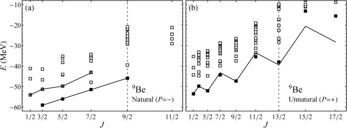
Figure 2: Energy eigenvalues obtained for states in the natural (left) and unnatural (right) parity spaces for $\isotope[9]{Be}$. Energies are plotted with respect to an angular momentum axis which is scaled to be linear in $J(J+1)$. Solid symbols indicate candidate yrast band members, and shaded symbols indicate candidate excited band members. Solid lines indicate the corresponding fits for rotational energies (2) (based on the first three band members for $K=1/2$ or all band members for $K=3/2$). Vertical dashed lines indicate the maximal angular momentum accessible within the lowest harmonic oscillator configuration (or valence space).

Energies following a rotational pattern are most easily recognized if plotted against an angular momentum axis which is scaled as $J(J+1)$, so that energies in an ideal rotational band lie on a straight line (or staggered about a straight line, for $K=1/2$). Such a plot of energies against angular momentum is shown for the calculated states of $\isotope[9]{Be}$ in Fig. 2, both for natural (negative) parity states (left) and unnatural (positive) parity states (right). (The parity of the lowest allowed oscillator configuration, or traditional shell model valence space, may be termed the natural parity, and that obtained by promoting one nucleon by one shell the unnatural parity.)

These calculations, from Ref. [10], are obtained taking a specific basis truncation ${N_{\text{max}}}=10$ (for natural parity, or ${N_{\text{max}}}=11$ for unnatural parity) and basis parameter ${\hbar\Omega}=22.5\,{\mathrm{MeV}}$ (near the variational minimum). They thus may be thought of as taking a snapshot of the spectrum along the path to convergence. These calculations are based on the realistic JISP16 nucleon-nucleon interaction [14]. The Coulomb interaction has been omitted, to ensure exact conservation of isospin, thereby simplifying the spectrum (we consider states of minimal isospin $T=T_{z}$ only). However, the effect of the Coulomb interaction, if included, is mainly to induce an overall shift in the binding energies.

Rotational bands are most readily identifiable near the yrast line, where the density of states remains comparatively low. Identification of band members is based not only on recognizing rotational energy patterns, but also on observing collective enhancement of electric quadrupole transition strengths among band members and verifying rotational patterns of electromagnetic moments and transitions. In the natural parity space [Fig. 2(a)], a $K=3/2$ yrast band (solid symbols) and $K=1/2$ excited band (shaded symbols) are identified, while, in the unnatural parity space [Fig. 2(b)], a $K=1/2$ yrast band is identified (solid symbols). For each of the candidate bands, the line indicates a rotational energy fit to the calculated band members.

Intriguing features of the bands found in the $\isotope{Be}$ isotopes relate to their termination at finite angular momentum. Some bands terminate at (or below) the maximal angular momentum permitted within the valence space, as in the case of both natural parity bands of $\isotope[9]{Be}$ [Fig. 2(a)]. [The maximal angular momentum permitted within the valence space (or lowest harmonic oscillator configuration) of each parity is indicated by the vertical dashed lines in Fig. 2.] However, some bands also extend beyond this angular momentum, as in the case of the unnatural parity yrast band of $\isotope[9]{Be}$ [Fig. 2(b)]. While this band deviates from the rotational energy formula above the maximal valence angular momentum, other calculated bands in the $\isotope{Be}$ isotopes continue through this angular momentum with no apparent deviation (see Ref. [10] for examples).

Figure 3: Dependence of calculated observables on the basis truncation ${N_{\text{max}}}$, for rotational band members in $\isotope[9]{Be}$: yrast and excited band energies, as (a) absolute energies $E$ and (c) excitation energies $E_{x}$, and yrast band electric quadrupole observables, both (b) quadrupole moments and (d) in-band transition matrix elements. Values are shown for successive ${N_{\text{max}}}$ truncations ($6\leq{N_{\text{max}}}\leq 10$) to provide an indication of convergence (calculations of increasing ${N_{\text{max}}}$ are indicated by plusses, crosses, and circles, respectively). Electric quadrupole moments and matrix elements are normalized to the intrinsic quadrupole moment $Q_{0}$, as determined from $Q(3/2)$. The curves indicate the values expected from the rotational formula. In panel (d), the upper and lower curves are for $\Delta J=2$ and $\Delta J=1$ transitions, respectively (for the definition and significance of the signs of these matrix elements, see Ref. [10]).

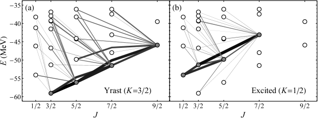
Figure 4: Calculated electric quadrupole transition matrix elements among states in the $\isotope[9]{Be}$ natural parity space: (a) from yrast band members and (b) from excited band members. In each panel, shaded circles indicate the initial levels being considered for transitions. All angular momentum decreasing transitions from the selected levels are shown. Line thicknesses are proportional to the magnitude of the reduced matrix element for the transition (also conveyed through a gray scale). Matrix elements are shown for the proton quadrupole tensor, but results with the neutron quadrupole tensor are similar.

Let us return to the challenge of convergence, now in relation to rotational patterns. The ${N_{\text{max}}}$ dependence of the energy eigenvalues, at fixed ${\hbar\Omega}=22.5\,{\mathrm{MeV}}$, is shown for the members of both natural parity bands in Fig. 3(a). For each step in ${N_{\text{max}}}$, the calculated energies shift lower by several ${\mathrm{MeV}}$. However, it may also be seen that the energies of different members of the same band move downward in approximate synchrony as ${N_{\text{max}}}$ increases. Thus, the energies within the band remain comparatively unchanged, as is seen more directly when we consider excitation energies in Fig. 3(c). The excitation energy of the excited band relative to the yrast band, though not converged, varies much less rapidly with ${N_{\text{max}}}$ than do the eigenvalues themselves.

The strengths of the various electric quadrupole transitions originating from the candidate band members in the natural parity bands of $\isotope[9]{Be}$ are shown in Fig. 4. We observe both the dominance of transitions within each band and the nonnegligible cross-talk between bands, as well as to some states outside these bands.

Although the calculated electric quadrupole observables are far from converged [Fig. 1(b)], rotational structure per se is reflected in the ratios of matrix elements within a band, not their absolute magnitudes, which depend also upon the intrinsic structure via $Q_{0}$ [see (3)]. In Fig. 3 (at right), we consider the calculated electric quadrupole matrix elements within the $\isotope[9]{Be}$ yrast band — quadrupole moments [Fig. 3(b)] and quadrupole transition matrix elements (both $\Delta J=1$ and $\Delta J=2$) [Fig. 3(d)] — and compare with the rotational predictions (lines). The overall normalization $Q_{0}$ is eliminated, by normalizing to the quadrupole moment of the band head [from which a value of $Q_{0}$ is determined by (3)]. Thus, rather than considering the unconverged matrix elements individually, as in Fig. 1(b), we effectively only consider ratios, of one unconverged matrix element to another. These normalized matrix elements are seen to be comparatively independent of ${N_{\text{max}}}$, at the ${N_{\text{max}}}$ values considered.

The resemblance between the calculated quadrupole moments and transition matrix elements and the expected rotational values (Fig. 1(b,d)), while clearly not perfect, is strongly suggestive of rotation. One should bear in mind that quadrupole moments of arbitrarily chosen states in the spectrum fluctuate not only in magnitude but also in sign, and that calculated transition matrix elements for arbitrarily chosen pairs of states fluctuate by many orders of magnitude [Fig. 4]. The rotational relation (3) is equally valid whether we take the quadrupole operator to be the proton quadrupole tensor (i.e., the physical electric quadrupole operator) $\boldsymbol{\mathbf{\mathrm{Q}}}_{p}$ or the neutron quadrupole tensor $\boldsymbol{\mathbf{\mathrm{Q}}}_{n}$. The matrix elements of these two operators, shown together in Fig. 3, provide valuable complementary information for investigating rotation. More extensive examples, including bands which extend to higher angular momentum, and considering magnetic dipole observables, may be found in Ref. [10].

Returning to the initial questions (from Sec. 1), now that we have explored how recognizable the signatures of rotation are, let us quantitatively examine how robust the rotational predictions are and how realistic they are in comparison to experiment. The energy parameters for bands across the $\isotope{Be}$ isotopic chain are summarized in Fig. 5: the band excitation energy $E_{x}$ (defined relative to the yrast band as $E_{x}\equiv E_{0}-E_{0,\text{yrast}}$), the band rotational parameter or slope $A$, and the band Coriolis decoupling parameter or staggering $a$ (for $K=1/2$). Results are shown for a sequence of ${N_{\text{max}}}$ truncations. Parameters for experimentally observed bands [15] are also shown (horizontal lines). (The calculations and experimental data are detailed in Ref. [10].)

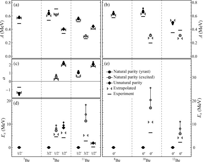
Figure 5: Band energy parameters for odd-mass $\isotope{Be}$ isotopes (left) and even-mass $\isotope{Be}$ isotopes (right): the rotational constant $A$ (top), Coriolis decoupling parameter $a$ (middle), and band excitation energy $E_{x}$ (bottom). Bands are distinguished as natural parity yrast (circles, solid), natural parity excited (circles, shaded), and unnatural parity yrast (diamonds). Values are shown for $6\leq{N_{\text{max}}}\leq 10$ for natural parity or $7\leq{N_{\text{max}}}\leq 11$ for unnatural parity, with larger symbols for higher ${N_{\text{max}}}$ values. Parameter values are also shown based on exponentially extrapolated level energies (paired triangles) and experimental bands (horizontal lines).

Our results for the rotational parameter $A$ and Coriolis decoupling coefficient $a$ [Fig. 5(a–c)] are sufficiently stable with respect to ${N_{\text{max}}}$ to permit at least a rough comparison with experiment. The value of the rotational parameter [Fig. 5(a,b)] varies by a factor of $\sim 2$ across the different calculated bands. The calculations reproduce both the general range of experimental values for $A$ and the general trend of which bands have higher or lower slopes (excepting $\isotope[12]{Be}$, where the discrepancies may arise due to mixing of the yrast and excited bands [16]). The Coriolis staggering for the calculated $K=1/2$ bands [Fig. 5(c)] varies in both amplitude and sign, and the experimental trend in both these properties is reproduced across the bands.

However, the excitation energies $E_{x}$ [Fig. 5(d,e)] converge at rates which vary considerably among the bands. In general, the excitation energies are decreasing with ${N_{\text{max}}}$, bringing them toward the experimental values. Yet, they are varying too strongly with ${N_{\text{max}}}$ for it to be immediately obvious how close the converged predictions will lie to the experimental values.

More detailed comparisons with the experimentally identified rotational bands could be made possible by the application of basis extrapolation methods [17, 18, 19], which are being developed to deduce the converged values for energies (and other observables). Such methods are still in their formative stages. Nonetheless, it is intriguing to apply a straightforward scheme based on a presumed exponential convergence of energy eigenvalues with ${N_{\text{max}}}$ [17]. The calculated energies are taken to approach the converged value $E_{\infty}$, for ${N_{\text{max}}}\rightarrow\infty$, as

$$E({N_{\text{max}}},{\hbar\Omega})=E_{\infty}+a_{{\hbar\Omega}}\exp(-b_{{\hbar\Omega}}{N_{\text{max}}}).$$ (4)

Calculations of the energy at three successive ${N_{\text{max}}}$ values, for fixed ${\hbar\Omega}$, are sufficient to determine all three parameters ($a_{{\hbar\Omega}}$, $b_{{\hbar\Omega}}$, and $E_{\infty}$) in (4) and thus provide an extrapolation to the converged energy.

Using extrapolated energies for the band members, we again determine the band energy parameters (paired triangles in Fig. 5), yielding results which match experiment to a greater (e.g., $\isotope[9]{Be}$ excitation energies) or lesser (e.g., $\isotope[10]{Be}$ excitation energy) degree. However, such extrapolations are subject to considerable uncertainties [17]. It is therefore not yet clear to what extent the remaining discrepancies reflect deficiencies in the ab initio description of the nucleus, with the chosen interaction (JISP16), or limitations of the exponential extrapolation.

In conclusion, we have seen that, despite the challenges of obtaining converged energies or electromagnetic observables, rotational patterns can robustly emerge in ab initio NCCI calculations, and these calculations can yield predictions of rotational properties for both qualitative and quantitative comparison with experiment. What remains to be addressed, from among our initial questions (in Sec. 1), is the physical origin and intrinsic structure of the rotation: prospective contributors include multishell $\mathrm{SU}(3)$ symmetry (shown to be dominant in NCCI calculations [6]), symplectic symmetry [20, 3], and $\alpha$-$\alpha$ molecular rotation [21].

Discussions with M. Freer are gratefully acknowledged. This work was supported by the US DOE under Grants No. DE-FG02-95ER-40934, DESC0008485 (SciDAC/NUCLEI), and DE-FG02-87ER40371, by the US NSF under Grant No. 0904782, and by the Research Corporation for Science Advancement Cottrell Scholar program. Computational resources were provided by the National Energy Research Scientific Computing Center (NERSC) and the Argonne Leadership Computing Facility (ALCF) (US DOE Contracts No. DE-AC02-05CH11231 and DE-AC02-06CH11357) and under an INCITE award (US DOE Office of Advanced Scientific Computing Research).

References

- [1] D. J. Rowe, Nuclear Collective Motion: Models and Theory (World Scientific, Singapore, 2010).
- [2] R. B. Wiringa, S. C. Pieper, J. Carlson, and V. R. Pandharipande, Phys. Rev. C 62, 014001 (2000).
- [3] T. Dytrych, K. D. Sviratcheva, C. Bahri, J. P. Draayer, and J. P. Vary, Phys. Rev. C 76, 014315 (2007).
- [4] T. Neff and H. Feldmeier, Eur. Phys. J. Special Topics 156, 69 (2008).
- [5] N. Shimizu, T. Abe, Y. Tsunoda, Y. Utsuno, T. Yoshida, T. Mizusaki, M. Honma, and T. Otsuka, Prog. Exp. Theor. Phys. 2012, 01A205 (2012).
- [6] T. Dytrych, K. D. Launey, J. P. Draayer, P. Maris, J. P. Vary, E. Saule, U. Catalyurek, M. Sosonkina, D. Langr, and M. A. Caprio, Phys. Rev. Lett. 111, 252501 (2013).
- [7] P. Maris, H. M. Aktulga, M. A. Caprio, U. V. Catalyurek, E. Ng, D. Oryspayev, H. Potter, E. Saule, M. Sosonkina, J. P. Vary, C. Yang, and Z. Zhou, J. Phys. Conf. Ser. 403, 012019 (2012).
- [8] P. Maris, J. Phys. Conf. Ser. 402, 012031 (2012).
- [9] M. A. Caprio, P. Maris, and J. P. Vary, Phys. Lett. B 719, 179 (2013).
- [10] P. Maris, M. A. Caprio, and J. P. Vary, Phys. Rev. C 91, 014310 (2015).
- [11] B. R. Barrett, P. Navrátil, and J. P. Vary, Prog. Part. Nucl. Phys. 69, 131 (2013).
- [12] M. A. Caprio, P. Maris, and J. P. Vary, Phys. Rev. C 90, 034305 (2014).
- [13] A. R. Edmonds, Angular Momentum in Quantum Mechanics, 2nd ed., Investigations in Physics No. 4 (Princeton University Press, Princeton, New Jersey, 1960).
- [14] A. M. Shirokov, J. P. Vary, A. I. Mazur, and T. A. Weber, Phys. Lett. B 644, 33 (2007).
- [15] H. G. Bohlen, W. von Oertzen, R. Kalpakchieva, T. N. Massey, T. Corsch, M. Milin, C. Schulz, Tz. Kokalova, and C. Wheldon, J. Phys. Conf. Ser. 111, 012021 (2008).
- [16] H. T. Fortune, G.-B. Liu, and D. E. Alburger, Phys. Rev. C 50, 1355 (1994).
- [17] P. Maris, J. P. Vary, and A. M. Shirokov, Phys. Rev. C 79, 014308 (2009).
- [18] S. A. Coon, M. I. Avetian, M. K. G. Kruse, U. van Kolck, P. Maris, and J. P. Vary, Phys. Rev. C 86, 054002 (2012).
- [19] R. J. Furnstahl, G. Hagen, and T. Papenbrock, Phys. Rev. C 86, 031301 (2012).
- [20] D. J. Rowe, Rep. Prog. Phys. 48, 1419 (1985).
- [21] Y. Kanada-En’yo, H. Horiuchi, and A. Doté, Phys. Rev. C 60, 064304 (1999).