Instability of a ferrimagnetic state of a frustrated $S=1/2$ Heisenberg antiferromagnet in two dimensions

Abstract

To clarify the instability of the ferrimagnetism which is the fundamental magnetism of ferrite, numerical-diagonalization study is carried out for the two-dimensional $S=1/2$ Heisenberg antiferromagnet with frustration. We find that the ferrimagnetic ground state has the spontaneous magnetization in small frustration; due to a frustrating interaction above a specific strength, the spontaneous magnetization discontinuously vanishes so that the ferrimagnetic state appears only under some magnetic fields. We also find that, when the interaction is increased further, the ferrimagnetism disappears even under magnetic field.

Ferrite is a magnetic material that is indispensable in modern society. It is because this material is used in various industrial products including motors, generators, speakers, powder for magnetic recording, and magnetic heads etc. It is widely known that fundamental magnetism of the ferrite is ferrimagnetism[1, 2, 3, 4]. The ferrimagnetism is an important phenomenon that has both ferromagnetic nature and antiferromagnetic nature at the same time. The occurrence of ferrimagnetism is understood as a mathematical issue within the Marshall-Lieb-Mattis (MLM) theorem[5, 6] concerning quantum spin systems. A typical case showing ferrimagnetism is when a system includes spins of two types that antiferromagnetically interact between two spins of different types in each neighboring pair, for example, an ($S$, $s$)=(1, 1/2) antiferromagnetic mixed spin chain, in which two different spins are arranged alternately in a line and coupled by the nearest-neighbor antiferromagnetic interaction. The ferrimagnetic state like the above case, in which the spontaneous magnetization is fixed to be a simple fraction of the saturated magnetization determined by the number of up spins and that of down spins in the state, is called the Lieb-Mattis (LM) type ferrimagnetism. Another example of ferrimagnetism is a system including single-type spins that are more than one in a unit cell, although the ferrimagnetism can appear even in a frustrating system including only a single spin within a unit cell[7, 8].

The antiferromagnet on the Lieb lattice illustrated in Fig. 1 corresponds the second case, in which there are three spins in a unit cell. The MLM theorem holds in the Lieb-lattice antiferromagnet. If antiferromagnetic interactions are added to this Lieb lattice so that magnetic frustrations occur, however, the MLM theorem no longer holds. In this situation, the ferrimagnetic state is expected to become unstable. The problem of how the ferrimagnetism collapses owing to such frustrating antiferromagnetic interactions is an important issue to understand the ferrimagnetism well and to make ferrimagnetic materials more useful in various products. This problem was studied in the $S=1/2$ Heisenberg antiferromagnet on the spatially anisotropic kagome lattice[9, 10], where the existence of an intermediate phase with weak spontaneous magnetization is clarified between the LM type ferrimagnetic phase and the nonmagnetic phase including the isotropic kagome-lattice antiferromagnet. We are then faced with a question: is there any other different behavior of the collapse of the ferrimagnetism?

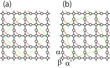
Figure 1: (Color) Network of antiferromagnetic interactions studied in this paper. The black and red bonds represent $J_{1}$ and $J_{2}$ interactions. Green squares denote finite-size clusters of 24 and 30 sites in (a) and (b), respectively. Note that the two-dimensional network composed only of the black bonds is called the Lieb lattice.

Under circumstances, the purpose of this study is to demonstrate the existence of a different behavior of collapsing ferrimagnetism in the case of an $S=1/2$ Heisenberg antiferromagnet on the lattice shown in Fig. 1 to answer the above question. When the antiferromagnetic interactions denoted by the red bonds vanish, the system is unfrustrated and thus it certainly shows ferrimagnetism in the ground state. In this study, we examine the case when the red-bond interactions are switched on.

The model Hamiltonian examined in this study is given by ${\cal H}={\cal H}_{0}+{\cal H}_{\rm Zeeman}$, where

$${\cal H}_{0} = \sum_{i\in{\alpha},j\in{\beta}}J_{1}\mbox{\boldmath$S$}_{i}\cdot\mbox{\boldmath$S$}_{j}+\sum_{i\in{\alpha^{\prime}},j\in{\beta}}J_{1}\mbox{\boldmath$S$}_{i}\cdot\mbox{\boldmath$S$}_{j}$$ (1)

$$+\sum_{i\in{\alpha},j\in{\alpha}^{\prime}}J_{2}\mbox{\boldmath$S$}_{i}\cdot\mbox{\boldmath$S$}_{j},$$

$${\cal H}_{\rm Zeeman} = -h\sum_{j}S_{j}^{z}.$$ (2)

Here $\mbox{\boldmath$S$}_{i}$ denotes an $S=1/2$ spin operator at site $i$. Sublattices $\alpha$, $\alpha^{\prime}$, and $\beta$ and the network of antiferromagnetic interactions $J_{1}$ and $J_{2}$ are depicted in Fig. 1. Here, we consider the case of isotropic interactions. The system size is denoted by $N_{\rm s}$. Energies are measured in units of $J_{1}$; thus, we take $J_{1}=1$ hereafter. We examine the properties of this model in the range of $J_{2}/J_{1}>0$. Note that, in the case of $J_{2}=0$, sublattices $\alpha$ and $\alpha^{\prime}$ are combined into a single sublattice; the system satisfies the above conditions of the MLM theorem. Thus, ferrimagnetism of the LM type is exactly realized in this case. In the limit of $J_{2}/J_{1}\rightarrow\infty$, on the other hand, the lattice of the system is reduced to a trivial system composed of isolated $S=1/2$ spins and isolated dimers of two spins. Its ground state is clearly different from the state of the LM-type ferrimagnetism in the case of $J_{2}=0$. One thus finds that while $J_{2}$ becomes larger, the ground state of this system will change from the ferrimagnetic one in the case of $J_{2}=0$ to another state, which we survey here.

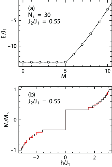
Figure 2: (Color) Results for $J_{2}/J_{1}=0.55$. Lowest energy in each subspace of $M$ for the system of $N_{\rm s}=30$ is shown in panel (a). The magnetization process is depicted in panel (b); red and black lines represent results for $N_{\rm s}=24$ and 30, respectively.

Next, we discuss the method we use here, which is numerical diagonalization based on the Lanczos algorithm[11]. It is known that this method is nonbiased beyond any approximations and reliable for many-body problems, which are not only localized spin systems such as the Heisenberg model[12, 13] treated in th present study but also strongly correlated electron systems including the Hubbard model[14, 15, 16] and the $t$-$J$ model[14, 17, 18]. A disadvantage of this method is that the available system sizes are limited to being small. Actually, the available sizes in this method are much smaller than those of the quantum Monte Carlo simulation[19, 20] and the density matrix renormalization group calculation[21]; however, it is difficult to apply both methods to a two-dimensional (2D) frustrated system like the present model. This disadvantage comes from the fact that the dimension of the matrix grows exponentially with respect to the system size. In this study, we treat the finite-size clusters depicted in Fig. 1 when the system sizes are $N_{\rm s}=24$ and 30 under the periodic boundary condition. Note that each of these clusters forms a regular square although cluster (b) is tilted from any directions along interaction bonds.

We calculate the lowest energy of ${\cal H}_{0}$ in the subspace characterized by $\sum_{j}S_{j}^{z}=M$ by numerical diagonalizations based on the Lanczos algorithm and/or the Householder algorithm. The energy is represented by $E(N_{\rm s},M)$, where $M$ takes every integer up to the saturation value $M_{\rm s}$ ($=SN_{\rm s}$). We here use the normalized magnetization $m=M/M_{\rm s}$. Some of Lanczos diagonalizations have been carried out using the MPI-parallelized code, which was originally developed in the study of Haldane gaps[22]. Note here that our program was effectively used in large-scale parallelized calculations[23, 24, 25].

To obtain the magnetization process for a finite-size system, one finds the magnetization increase from $M$ to $M+1$ at the field

$$h=E(N_{\rm s},M+1)-E(N_{\rm s},M),$$ (3)

under the condition that the lowest-energy state with the magnetization $M$ and that with $M+1$ become the ground state in specific magnetic fields. Note here that it often happens that the lowest-energy state with the magnetization $M$ does not become the ground state in any field. The magnetization process in this case is determined around the magnetization $M$ by the Maxwell construction[26, 27].

Now, we observe the case of $J_{2}/J_{1}=0.55$; results are shown in Fig. 2. Figure 2(a) depicts the lowest energy level in the subspace belonging to $M$ for $N_{\rm s}=30$. The levels for $M=0$ to $M=5$ are identical within the numerical accuracy. For $M>5$, the energies increase with $M$. This behavior indicates that the spontaneous magnetization is $M=5$. In Fig. 2(b), we draw the magnetization process determined by eq. (3) in the full range from the negative to the positive saturations. The spontaneous magnetization $m=1/3$ appears and the state at $m=1/3$ shows the plateau with a large width. It is observed that, above $m=1/3$, the magnetization grows continuously. These behaviors are common with those of the LM ferrimagnetism at the unfrustrated case of $J_{\rm 2}=0$.

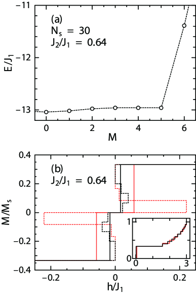
Figure 3: (Color) Results for $J_{2}/J_{1}=0.64$. Lowest energy in each subspace of $M$ for the system of $N_{\rm s}=30$ is shown in panel (a). The magnetization process is depicted in panel (b); red and black lines represent results for $N_{\rm s}=24$ and 30, respectively. Main panel is a zoomed-in view of its inset with a wide range. The broken lines represent the results before the Maxwell construction is carried out.

Next, let us examine the case of $J_{2}/J_{1}=0.64$; results are shown in Fig. 3. The $M$ dependence of the lowest energy belonging to $M$ is different in $M<3$ from the case of $J_{2}/J_{1}=0.55$. This difference affects with the disappearance of the spontaneous magnetization, which is shown in Fig. 3(b). This discontinuous disappearance occurs at $J_{2}/J_{1}\sim 0.59$ for $N_{\rm s}=24$ and at $J_{2}/J_{1}\sim 0.63$ for $N_{\rm s}=30$. An important point is that an intermediate state with smaller but nonzero spontaneous magnetizations is absent between the $m=1/3$ state and the nonmagnetic state. This behavior is clearly different from the presence of such an intermediate state in the spatially anisotropic kagome lattice[9, 10]. We speculate that this difference comes from the point that the competing interaction in the present model has a strong quantum nature localized at pairs of dimerized spins. The discovery of the future third case of the collapsing ferrimagnetism would contribute to confirm our speculation. Note also that the plateau at $m=1/3$ shows a large width. This suggests that the ferrimagnetic state is realized if external magnetic fields are added.

To examine the properties of the $m=1/3$ states in a more detailed way, we evaluate the local magnetization defined as

$$m_{\rm LM}^{\xi}=\frac{1}{N_{\xi}}\sum_{j\in\xi}\langle S_{j}^{z}\rangle,$$ (4)

where $\xi$ takes $\alpha$, $\alpha^{\prime}$ and $\beta$. Here, the symbol $\langle{\cal O}\rangle$ denotes the expectation value of the operator ${\cal O}$ with respect to the lowest-energy state within the subspace with a fixed $M$ of interest. Recall here that the case of interest in this paper is $M=M_{\rm s}/3$. Here $N_{\xi}$ denotes the number of $\xi$ sites. Results are shown in Fig. 4. In the region of small $J_{2}/J_{1}$, $\alpha$ and $\alpha^{\prime}$ spins are up and $\beta$ spin is down, although each of magnetizations is slightly deviated from the full moment due to a quantum effect. This spin arrangement is a typical behavior of ferrimagnetism. On the other hand, in the region of large $J_{2}/J_{1}$, the magnetizations at $\alpha$ and $\alpha^{\prime}$ spins are vanishing and $\beta$ spin shows almost a full moment up. This marked change in the local magnetizations occurs at $J_{2}/J_{1}\sim 1.38$ for $N_{\rm s}=24$ and at $J_{2}/J_{1}\sim 1.40$ for $N_{\rm s}=30$, which suggests the occurrence of the phase transition around at $J_{2}/J_{1}\sim 1.4$. Therefore one finds that, for $J_{2}/J_{1}$ larger than this transition point, the ferrimagnetic state cannot be realized even under magnetic fields. It is unfortunately difficult to determine the transition point in the thermodynamic limit precisely only from the present two samples of small clusters. For the determination, calculations of larger clusters are required in future studies. Note here that similar observations of the local magnetizations were reported in Refs. References and References, which treated the Heisenberg antiferromagnet on the Cairo-pentagon lattice [30], a 2D network obtained by the tiling of single-kind inequilateral pentagons. The same behavior of $m_{\rm LM}^{\xi}$ is also observed when the kagome-lattice antiferromagnet[31, 32, 33, 34, 35, 36, 37] is distorted in the $\sqrt{3}\times\sqrt{3}$ type[25, 38]. The relationship between these models should be examined in future studies. Note also that, in the present model, the change around the transition point seems continuous irrespective of whether the system size is $N_{\rm s}=24$ or 30. This aspect is different from the observation in the Cairo-pentagon-lattice antiferromagnet[28, 29], where the change around the transition point seems continuous for $N_{\rm s}=24$ but discontinuous for $N_{\rm s}=30$. We speculate that whether the change is continuous or discontinuous in finite-size data is related to whether the number of unit cells in finite-size clusters is an even integer or an odd integer. To confirm this speculation, further investigations are required in future. It will be an unresolved question whether the transition is continuous or discontinuous in the thermodynamic limit. Figure 5 depicts the magnetization process at $J_{2}/J_{1}\sim 1.39$. No jumps seem to appear in the process at $J_{2}/J_{1}$ corresponding to the transition point. It is unclear whether the width at $m=1/3$ survives or vanishes although this $m=1/3$ width at $J_{2}/J_{1}\sim 1.39$ is smaller than those in Figs. 2(b) and 3(b). Future studies would clarify how the magnetization process behaves in the vicinity of the transition point.

In summary, we have investigated how the ferrimagnetic state of the $S=1/2$ Heisenberg antiferromagnet on the 2D lattice collapses owing to magnetic frustration by numerical-diagonalization method. We capture a discontinuous vanishing of the spontaneous magnetization without intermediate phase showing spontaneous magnetizations that are smaller than that of the Lieb-Mattis ferrimagnetic state when a frustrating interaction is increased. We also observe the disappearance of the ferrimagnetic state under magnetic fields for even larger interaction showing frustration. It is known that organic molecular magnets can realize ferrimagnetism[39, 40]. Since variety of lattice structure leading to an interaction network is available in such organic molecular magnets, the experimental confirmation might be done in these magnets more easily than metallic-element compounds. Further studies concerning instability of the ferrimagnetism would contribute much for our development of more stable ferrimagnetic materials.

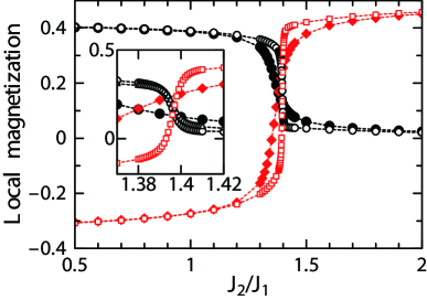
Figure 4: (Color) Behavior of local magnetizations vs. the ratio of interactions $J_{2}/J_{1}$ together with a zoomed-in view near the transition point in inset. Closed circles and closed diamonds denote results for $\alpha$ and $\beta$ for $N_{\rm s}=24$, respectively. Results for $\alpha^{\prime}$ for $N_{\rm s}=24$ are identical those for $\alpha$ within the numerical accuracy because $\alpha$ and $\alpha^{\prime}$ are symmetric in the $N_{\rm s}=24$ cluster. Open circle, open triangle, and open squares represent results for $\alpha$, $\alpha^{\prime}$, and $\beta$ for $N_{\rm s}=30$, respectively. Due to the tilting for $N_{\rm s}=30$, $\alpha$ and $\alpha^{\prime}$ are not symmetric, although results of $\alpha$ and $\alpha^{\prime}$ for $N_{\rm s}=30$ are slightly different but very similar. To avoid invisibility from overlapping of symbols, results of $\alpha^{\prime}$ are shown only in inset.

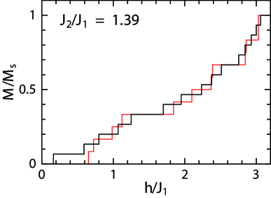
Figure 5: (Color) Magnetization process for $J_{2}/J_{1}=1.39$. Red and black lines represent results for $N_{\rm s}=24$ and 30, respectively.

- [1] N. Ichinose, Jpn. J. Appl. Phys. 5, 461 (1966).
- [2] N. Ichinose, Jpn. J. Appl. Phys. 5, 1140 (1966).
- [3] A. M. Blanco and F. C. Gonzalez, J. Phys. D 22, 210 (1989).
- [4] R. Heindl,R. Deschamps, M. Domine-Berges, and J. Loriers, J. Magn. Magn. Mater. 7, 26 (1978).
- [5] W. Marshall, Proc. R. Soc. London, Ser. A 232, 48 (1955).
- [6] E. Lieb and D. Mattis, J. Math. Phys. (N.Y.) 3, 749 (1962).
- [7] T. Shimokawa and H. Nakano, J. Phys. Soc. Jpn. 80, 043703 (2011).
- [8] T. Shimokawa and H. Nakano, J. Phys. Soc. Jpn. 80, 125003 (2011).
- [9] H. Nakano, T. Shimokawa, and T. Sakai, J. Phys. Soc. Jpn. 80, 033709 (2011).
- [10] T. Shimokawa and H. Nakano, J. Phys. Soc. Jpn. 81, 084711 (2012).
- [11] C. Lanczos, J. Res. Natl. Bur. Stand. 45, 255 (1950).
- [12] J. B. Parkinson and J. C. Bonner, Phys. Rev. B 32, 4703(1985).
- [13] H. Q. Lin, Phys. Rev. B 42, 6561 (1990)
- [14] A. Moreo and E. Dagotto, Phys. Rev. B 42, 4786 (1990).
- [15] E. Dagotto, A. Moreo, F. Ortolani, D. Poilblanc, and J. Riera, Phys. Rev. B 45, 10741 (1992).
- [16] H. Nakano, Y. Takahashi, and M. Imada, J. Phys. Soc. Jpn. 76, 034705 (2007).
- [17] M. Ogata, M. U. Luchini, S. Sorella, and F. F. Assaad, Phys. Rev. Lett. 66, 2388 (1991).
- [18] H. Tsunetsugu and M. Imada, J. Phys. Soc. Jpn. 67, 1864 (1998).
- [19] S. Miyashita, J. Phys. Soc. Jpn. 57, 1934 (1988).
- [20] S. Todo and K. Kato, Phys. Rev. Lett. 87, 047203 (2001).
- [21] S. R. White and D. A. Huse, Phys. Rev. B 48, 3844 (1993).
- [22] H. Nakano and A. Terai, J. Phys. Soc. Jpn. 78, 014003 (2009).
- [23] H. Nakano and T. Sakai, J. Phys. Soc. Jpn. 80, 053704 (2011).
- [24] H. Nakano, S. Todo, and T. Sakai, J. Phys. Soc. Jpn. 82, 043715 (2013).
- [25] H. Nakano and T. Sakai, J. Phys. Soc. Jpn. 83, 104710 (2014).
- [26] M. Kohno and M. Takahashi, Phys. Rev. B 56, 3212 (1997).
- [27] T. Sakai and M. Takahashi, Phys. Rev. B 60, 7295 (1999).
- [28] H. Nakano, M. Isoda, and T. Sakai, J. Phys. Soc. Jpn. 83, 053702 (2014).
- [29] M. Isoda, H. Nakano, and T. Sakai, J. Phys. Soc. Jpn. 83, 084710 (2014).
- [30] I. Rousochatzakis, A. M. Luchli, and R. Moessner, Phys. Rev. B 85, 104415 (2012).
- [31] P. Lecheminant, B. Bernu, C. Lhuillier, L. Pierre, and P. Sindzingre, Phys. Rev. B 56, 2521 (1997).
- [32] C. Waldtmann, H.-U. Everts, B. Bernu, C. Lhuillier, P. Sindzingre, P. Lecheminant, and L. Pierre, Eur. Phys. J. B 2, 501 (1998).
- [33] K. Hida, J. Phys. Soc. Jpn. 70, 3673 (2001).
- [34] J. Schulenburg, A. Honecker, J. Schnack, J. Richter, and H.-J. Schmidt, Phys. Rev. Lett. 88, 167207 (2002).
- [35] P. Sindzingre and C. Lhuillier, Europhys. Lett. 88, 27009 (2009).
- [36] H. Nakano and T. Sakai, J. Phys. Soc. Jpn. 79, 053707 (2010).
- [37] T. Sakai and H. Nakano, Phys. Rev. B 83, 100405(R) (2011).
- [38] H. Nakano, T. Sakai, Y. Hasegawa, J. Phys. Soc. Jpn. 83, 084709 (2014).
- [39] Y. Hosokoshi, K. Katoh, Y. Nakazawa, H. Nakano, and K. Inoue, J. Am. Chem. Soc. 123, 7921 (2001)
- [40] Y. Hosokoshi, K. Katoh, K. Inoue, Synth. Met. 133, 527 (2003).