Improvements of the shock arrival times at the Earth model STOA

Abstract

Prediction of the shocks’ arrival times (SATs) at the Earth is very important for space weather forecast. There is a well-known SAT model, STOA, which is widely used in the space weather forecast. However, the shock transit time from STOA model usually has a relative large error compared to the real measurements. In addition, STOA tends to yield too much ‘yes’ prediction, which causes a large number of false alarms. Therefore, in this work, we work on the modification of STOA model. First, we give a new method to calculate the shock transit time by modifying the way to use the solar wind speed in STOA model. Second, we develop new criteria for deciding whether the shock will arrive at the Earth with the help of the sunspot numbers and the angle distances of the flare events. It is shown that our work can improve the SATs prediction significantly, especially the prediction of flare events without shocks arriving at the Earth.

Gindraft=false LIU and QIN Improvements on STOA H.-L. Liu, State Key Laboratory of Space Weather, Center for Space Science and Applied Reaserch, Chinese Academy of Sciences, P.O. Box 8701, Beijing 100190, China. (hlliu@spaceweather.ac.cn) G. Qin, State Key Laboratory of Space Weather, Center for Space Science and Applied Reaserch, Chinese Academy of Sciences, P.O. Box 8701, Beijing 100190, China. (gqin@spaceweather.ac.cn)

1 Introduction

Interplanetary shocks are among the products of eruptive solar events, and they can also accelerate energetic particles which influence the geo-space environment seriously. So predicting of the shock arrival times (SATs) at Earth is a necessary step for space weather forecast system. Coronal shock waves are counterparts of the interplanetary shocks in corona. The coronal shock waves’ origin is still questionable, but generally two eruptive phenomena from the Sun are thought to be responsible: flares and coronal mass ejections (CMEs) (Vr$\check{s}nak$ and Cliver, 2008). So most prediction models take the observation data of flares or CMEs as their inputs. Although CMEs are usually associated with flaress (Dryer, 1996), in this paper we mainly focus on the shocks related with solar flare eruption events.

Among many models built to predict the eruption-driven shock events, there are three famous physics-based eruption-driven shock SAT prediction models, the Shock Time of Arrival (STOA) model (Dryer and Smart, 1984; Smart and Shea, 1985), the Interplanetary Shock Propagation Model (ISPM) (Smith and Dryer, 1990), and the Hakamada-Akasofu-Fry Version 2 (HAFv.2) Model (Fry et al., 2001), which are used widely and referred as 3PMs hereafter. Afterwards, many other SAT prediction models are developed (e.g., Feng and Zhao, 2006; Feng et al., 2009a, b; Qin et al., 2009; Liu and Qin, 2012). For the prediction of CMEs-related shocks, please refer to Zhao and Dryer (2014).

It is shown that 3PMs use the same observation data as inputs. As numerical simulation models considering more physics mechanisms, ISPM and HAFv.2 are more complicated than STOA, which is an analytical model. Especially, the HAFv.2 model is rather complicated, which simulates the magnetic fields in solar wind with the effects of the transitions of shocks. ISPM is based on 2.5 MHD simulation, and HAFv.2 is calibrated with 1D and 2D MHD simulation (Sun et al., 1985). So, STOA is relatively easier to operate and optimize, but its performance is not inferior to ISPM and HAFv.2 models (Fry et al., 2003; McKenna-Lawlor et al., 2006). In practice, the STOA model is used most extensively among 3PMs.

Transit time of the shock is an important output for SAT prediction models. STOA yields $12$ hours root mean square (RMS) error for $\Delta T$ (difference between predicted transit time $T_{pre}$ and observed transit time $T_{obs}$). Besides other effects, the inaccuracy of the input parameters contribute to the forecast errors of SAT prediction models. Zhao and Feng (2014) built a new prediction model SPM2 by adjusting the input parameters of SPM model, and SPM2 performed better than SPM. In STOA model, shock is assumed to ride over an isotropic background solar wind plasma flow, so the speed ($V_{sw}$) of the flow is one of the input parameters of STOA. However, the shock goes through background solar wind flow with varying $V_{sw}$ during its propagation from the Sun to the observer, and no observation techniques at present could provide $V_{sw}$ accurately over the whole path route of the shock. Furthermore, the $1$ AU solar wind velocity at the time of the parent flare event’s eruption is used as the speed of the flow in STOA. It is possible to improve the prediction of STOA by providing more reasonable value of $V_{sw}$.

Not all the coronal shocks would arrive at Earth, eg., some of them may decay to MHD waves which are relatively harmless to the electronic instruments. So a model to predict SATs should use some criterion to predict whether the shock will arrive at Earth before predicting the shock’s transit time. STOA uses a simplified magnetoacoustic Mach number $M_{\alpha}$ at $1$ AU to represent the strength of the shock. If $M_{\alpha}$ is greater than $1.0$ the model will provide the ‘yes’ prediction which means there will be a shock observed at Earth, otherwise the model provides the ‘no’ prediction. In practice, false ‘no’ prediction may bring damage to satellites in space and some electronic instruments on the ground, and false ‘yes’ prediction may lead to extra expenses on operation of the instruments and discontinuities of science observations. It is shown that STOA model tends to provide too much ‘yes’ prediction (McKenna-Lawlor et al., 2006).

Some research about the criterion for SATs prediction models had been done. Solar flare eruption events not only produce coronal shocks but also emit high energy particles. Qin et al. (2009) used the $38-53$ KeV electrons observed by EPAM/ACE at $1$ AU to help predicting whether the shock will arrive at Earth. New method given by Qin et al. (2009) improved the prediction of the SATs significantly. Liu and Qin (2012) developed a new SATs prediction method (STOASF) with the help of energy released by flare in soft X-ray. It is shown that the new method STOASF performs much better than STOA on those events without shock arrivals at Earth (Liu and Qin, 2012).

We build four new SATs prediction methods in this paper. We first describe the data and events used in section 2. In Section 3, we introduce some new methods to predict SATs. In section 4, we compare the performances of different prediction methods. We discuss and summarize our results in section 5.

2 Data and Events Selection

The parent solar flare eruption events and their corresponding shocks observations at $1$ AU used in our work are from the combination of the lists in Fry et al. (2003), McKenna-Lawlor et al. (2006) and Smith et al. (2009). There are $625$ flare events altogether in the three papers, which cover the period of the whole Solar Cycle 23 from February 1997 to December 2006. The whole data set used in our work is from real time experience unlike the other models regardless of their scientific sophistication. STOA only consider the flare energy released during the solar eruption events, so it made made prediction of the SATs without considering CMEs data(Smith et al., 2000). Smith et al. (2009) matched CMEs observation data for the event set used in their work and tested the performance of the HAFv.2 model. No CMEs data were included in Fry et al. (2003) and McKenna-Lawlor et al. (2006). In our work, we still don’t take account of CMEs. Start times of the metric type II coronal events are taken as the begin times of these parent solar flare eruption events, and the duration are derived from the GOES X-ray flux. Optical flare observation data provides the location of the parent events. The corresponding shocks data at L1 are from ACE, SOHO or WIND. Matching of the parent eruption events and shocks at Earth will be a little different for each model. Here we use the matches that are most favourable for STOA.

We only use $582$ events in our study, which means $43$ events are excluded from the list mentioned in the last paragraph. Qin et al. (2009) excluded $3$ events because of the lack of $0.038-0.053$ MeV energetic electrons data observed by ACE/EPAM. And another $37$ events with soft X-ray intensity data unavailable were further removed from the work of Liu and Qin (2012). In this paper we remove additional $3$ events with abnormal observed transit times, which leaves $582$ events finally. Hereafter, we denote the $582$ events used in this paper as $E_{582}$. The fearless forecast numbers of the $43$ events removed from the combination of the lists in Fry et al. (2003), McKenna-Lawlor et al. (2006) and Smith et al. (2009) are shown in table 1. Out of the $582$ flare events we use here, $225$ are accompanied with shocks at Earth, which are named as ‘with shock’ (WS) events, and the rest $357$ events without shock at Earth are named as ‘without shock’ (WOS) events.

3 New Prediction Methods

In the following, we describe some new prediction methods of SATs. The detailed performances check of the methods will be shown in Section 4.

3.1 Replacing Solar Wind Speed with a Typical Constant $V_{c}$, a New Prediction Method STOA^′

In STOA model, the background solar wind speed ($V_{sw}$) over the whole path route of the shock is very important for the calculation of the transit time. But there is no way to observe such quantity accurately. So STOA used $1$ AU solar wind speed at the time of flare events’ eruption instead. This process may yield large errors because of the spacial and temporal perturbations of the solar wind.

Therefore, we use a constant $V_{c}$ to represent the typical value of solar wind speed over the shock journey for simplicity purpose, and a modification of the STOA model is obtained. We average solar wind speed over the $E_{582}$ as $\overline{V}_{sw}=455$ km/s. So we can set $V_{c}=455$ km/s and the modified STOA model is denoted as STOA^′. It should be noted that the input parameters of the STOA^′ are the same as STOA except that $V_{sw}$ is replaced by $V_{c}=455$ km/s in STOA^′. Furthermore, in STOA^′, we still use $M_{\alpha}$ defined by STOA to measure the strength of the shock at $1$ AU, and only when $M_{\alpha}>1.0$ would the shock arrive at the Earth. Since $V_{sw}$ is not needed to calculate $M_{\alpha}$ in STOA, the criterion of STOA^′ is the same as that of STOA.

3.2 Using Sunspot Number (SSN) to Help Predicting the SATs at Earth, a New Prediction Method STOASSN

When using the $E_{582}$ to test performance of STOA’s criterion, we found that STOA model tends to yield too much ‘yes’ prediction. There are $225$ of the $582$ flare events followed by shocks at Earth, but STOA model yields $438$ ‘yes’ prediction, which may imply that STOA underestimates the decay of shocks by various structures in solar wind while propagating through the interplanetary space. In addition, there are more structures with stronger solar activity, which can be indicated by the sunspot number (SSN). Therefore, we introduce a new parameter $M_{\alpha}^{SSN}$ to modify $M_{\alpha}$ of STOA with the help of SSN,

$$M_{\alpha}^{SSN}=\frac{M_{\alpha}}{k_{SSN}\overline{SSN}+b_{SSN}}$$ (1)

where $k_{SSN}$ and $b_{SSN}$ are constants, and $\overline{SSN}$ is the average of daily sunspot number during a time period before the flare event. To get a reasonable $\overline{SSN}$, the time period for average of daily sunspot numbers is very important. A too long period would introduce the effects of other solar eruption events which are not related to the shock events. Here we use $10$ day before the flare event as the time period to get the $\overline{SSN}$. We can adjust the values of $k_{SSN}$, $b_{SSN}$ to get different models. Using the $E_{582}$ we can check the performances of the models. Hereafter we use $k_{SSN}=0.006$ and $b_{SSN}=1.1$ which are the best parameters we can get so far. Note that the daily sunspot number data are from http://sidc.oma.be/html/dailyssn.html.

By modifying the $M_{\alpha}$ of STOA as $M_{\alpha}^{SSN}$ we can get a new SATs prediction method, STOASSN. So the criterion of STOASSN is different than STOA, but the transit time of STOASSN is the same as that of STOA.

3.3 A New SATs prediction model, STOASSN^′, Which Combines STOA^′ and STOASSN

Here we introduce a new model STOASSN^′ by combining two new models, STOA^′ and STOASSN. In STOASSN^′ model, the background solar wind speed $V_{sw}$ is replaced by typical constant $V_{c}=455$ km/s, and meanwhile the $M_{\alpha}^{SSN}$ is used as the criterion to decide whether the shock will arrive at the Earth. If $M_{\alpha}^{SSN}>1.0$, then a ‘yes’ prediction will be given, which means a shock is going to impact the Earth, while if $M_{\alpha}^{SSN}\leq 1.0$ then no shock will arrive at the Earth.

3.4 Using the Flare Events’ Angle Distance to Help Predicting the SATs at Earth, a New Prediction Method STOAAD

The angle distance $\phi$ between the shock’s nose propagation direction and the Sun-Earth line is also important for SATs prediction. It is known that shock nose is the strongest part of shock front, and the shock strength decreases by increasing solid angle distance from shock nose. In STOA model, shock nose is assumed to be in the direction of the parent flare event. Therefore, the angle distance $\phi$ can be calculated from the equation $\cos(\phi)=\cos(\theta)\cos(\varphi)$, where $\theta$ and $\varphi$ are the central meridian diastance and latitude of the solar flare events, respectively. Larger angle distance ($\phi$) means that the observer is far away from the shock nose direction and the chance to observe a shock is smaller. In addition, flare events with higher energy may drive a stronger coronal shock which is not easy to decay to MHD wave. Liu and Qin (2012) used the effects of energy released in soft X-ray during the flare events, $E_{x}^{\prime}$, to help to decide if shock would arrive at Earth.

Therefore, we build a new criterion by combining the effects of energy $E_{x}^{\prime}$ and the angle distance $\phi$. Note that in Liu and Qin (2012) the energy $E_{x}^{\prime}$ could be negative. Here in order to keep $E_{x}^{\prime}$ positive for convenience, we redefine the $E_{x}^{\prime}$ as,

$$E_{x}^{\phi}=f\tau,$$ (2)

where $f$ is the peak intensity of soft X-ray during the flare event, and $\tau$ is the duration time of the event.

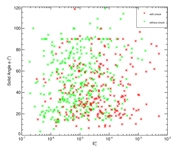
Figure 1: Distribution of $582$ events with the energy $E_{x}^{\phi}$ and the angle distance $\phi$

Figure 1 shows $E_{x}^{\phi}$ versus $\phi$ of the $E_{582}$. Here we use stars with different colors to represent the two type events, red for WS events (the flare events that are accompanied by shocks at Earth) and green for WOS events (the flare events that are not accompanied by shocks at Earth). It is shown that the WOS events tend to locate in the top left corner of the figure, and the WS events are more likely to locate in the bottom right corner.

Based on the above analysis, we combine the effects of $E_{x}^{\phi}$ and the angle distance $\phi$ to introduce a new criterion for predicting the SATs,

$$C_{x}^{\phi}=-\lg\left(\frac{E_{x}^{\phi}}{E_{x0}^{\phi}}\right)\left(\frac{\phi}{10}\right)^{b},$$ (3)

here $E_{x0}^{\phi}=1$ Whr/m² is a constant and $E_{x}^{\phi}$ is always smaller than $E_{x0}^{\phi}$. Equation 3 shows a negative relationship between $E_{x}^{\phi}$ and $C_{x}^{\phi}$ and a positive relationship between $\phi$ and $C_{x}^{\phi}$. It is possible the two kinds of events, WS events and WOS events, can be separated according to the value of $C_{x}^{\phi}$. We tried different values of $b$ in Equation 3 and found that $b=0.1$ could make the best results for the $E_{582}$.

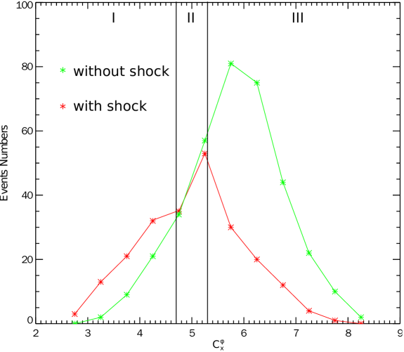
Figure 2: Distribution of events’ numbers with $C_{x}^{\phi}$

Figure 2 shows the number of flare events in different intervals of $C_{x}^{\phi}$ with the same range $0.5$. Red and green symbols represent WS and WOS events, respectively. The two vertical lines, $C_{x}^{\phi}=4.7$ and $C_{x}^{\phi}=5.3$, divide the x-axis into three regions. It is shown that there are more WS events than WOS events with $C_{x}^{\phi}<4.7$ (Region I), which means that shock events in such condition are more likely to arrive at Earth, but in contrast most flare events with $C_{x}^{\phi}>5.3$ (Region III) are not accompanied by shocks at Earth. In addition, with $4.7\leq C_{x}^{\phi}\leq 5.3$ (Region II), the ratio of WS events number and WOS events number is close to $1$, which implies the probability for a shock to be detected at Earth is $50\%$. We take different methods to predict whether the shock will arrive at Earth in the three $C_{x}^{\phi}$ intervals. In STOA model, only the shocks with $M_{\alpha}>1.0$ will arrive at the Earth. We lower the threshold of $M_{\alpha}$ in Region I. In this region, if $M_{\alpha}>0.8$, a ‘yes’ prediction will be provided. However, a larger threshold for $M_{\alpha}$, $1.5$, is used in region III, which means that only if $M_{\alpha}>1.5$ a ‘yes’ prediction will be provided. In region II, furthermore, we adopt the STOASEP model because its performance on WS events and WOS events are equal. Here, the new method developed is named STOAAD.

4 Performances of the New Methods

Some variables are used to test the performances of SATs prediction models. The four parameters, hits (h), misses (m), false alarms (fa), and correct nulls (cn) are used to express the success or failure of the forecasts. In addition, success rate (sr), is an important parameter for the evaluation of SATs prediction models. But a prediction model with high value of sr does not necessarily guarantee it a good model. Standard meteorological skills are introduced to help evaluating the performances of the prediction models. Definitions or calculations of these variables are listed as follows,

• Hit (h), shock is predicted and observed at the Earth within $\pm 24$ hours

• Miss (m), shock is observed but not predicted within $1\sim 5$ days of the solar flare event or shock is predicted and observed but not $\pm 24$ hours

• False Alarm (fa), shock is predicted but not observed within $\pm 24$ hours

• Correct Null (cn), shock is not predicted and no one is observed within $1\sim 5$ days of the solar flare event

• Success Rate (sr), (h+cn)/(h+m+fa+cn)

• Probability of detection, yes (PODy), h/(h+m)

• Probability of detection, no (PODn), cn/(fa+cn)

• False alarm ratio (FAR), fa/(h+fa)

• Bias, (h+fa)/(h+m)

• Critical success index (CSI), h/(h+fa+m)

• True skill score (TSS), PODy+PODn-1

• Heidke skill score (HSS), (h+cn-C1)/(N-C1)

• Gilbert skill score (GSS), (h-C2)/(h+fa+m-C2)

where N (N=h+m+fa+cn) is the total number of events used in our study, C2=(h+m)(h+fa)/(N), and C1=C2+(fa+cn)(m+cn)/N. The $E_{582}$ and their corresponding observations at Earth described in section 2 are used to test the performances of STOA and other four new models, STOA^′, STOASSN, STOASSN^′, and STOAAD.

It can be seen from table 2 that STOA^′ and STOA nearly yield the same results, but STOA^′ predicts one more WS event correctly than STOA does. The new models STOASSN, STOASSN^′ and STOASD miss more shock events than STOA does, but they correctly predict more WOS events than STOA does. So the number of correct nulls yielded by the three of them is much larger than that by STOA and STOA^′. There are $357$ (fa+cn) WOS events among the $E_{582}$, but STOA and STOA^′ only correctly predict $35\%$ of the WOS events, or $126$ events. STOASSN, STOASSN^′ and STOAAD perform much better for the WOS events, with correct nulls $235$, $235$ and $201$, respectively. The last column in table 2 shows the success rates of each models. The sr of STOASSN and STOASSN^′ are $65\%$, which are the highest among the four models, and the sr of STOA yields the lowest value of $0.51$.

Table 3 shows comparison of STOA and STOA^′ in terms of the forecast errors $\Delta T$. Among the $E_{582}$, there are $225$ WS events, for which the root mean square errors of $\Delta T$, $RMS_{\Delta T}(all)$, are listed in column 2 of table 3. The $RMS_{\Delta T}(all)$ of STOA and STOA^′ are $18.96$ hours and $17.89$ hours, respectively. Column 3 shows the number of events with $|\Delta T|\leq 48$ hours. For STOA and STOA^′, $220$ and $222$ events are with $|\Delta T|\leq 48$ hours, respectively. In addition, the root mean square errors of $|\Delta T|\leq 48$ hours events are $17.21$ hours and $16.52$ hours for STOA and STOA^′, respectively. It is shown that the new method STOA^′ not only provides prediction with more events with $|\Delta T|\leq 48$ hours, but also gets smaller $RMS_{\Delta T}$. STOA^′ also performs better than STOA does with events with $|\Delta T|\leq 24$ hours. We also find that among the $225$ flare events accompanied with shocks at the Earth, STOA^′ provides better transit time for $124$ events. So statistically STOA^′ provides better forecast for the data set used in our study.

Table 4 shows the performances of the four different SATs prediction models: STOA, STOA^′, STOASSN and STOAAD, in terms of standard meteorological forecast skill scores. PODy implies a SATs model’s performance with WS events that are predicted correctly. PODy of STOA equals $0.77$ means that STOA forecasts $77\%$ of the WS events successfully. PODy of STOA^′ equals $78\%$, which is roughly the same as that of STOA. But STOASSN, STOASSN^′ and STOAAD have less hits with WS events, so PODy of them are lower, which are $0.63$, $0.64$ and $0.66$, respectively. Among the $E_{582}$, there are $357$ WOS events. So it is essential for an SATs prediction model to provide satisfactory prediction for WOS events in practice. The second parameter PODn in table 4 represents the proportion of WOS events that are predicted correctly. The models STOA and STOA^′ still have the same performance in terms of PODn. The PODn of other three models, STOASSN, STOASSN^′, and STOAAD, are $0.66$, $0.66$ and $0.56$, respectively, which means that STOASSN and STOASSN^′ perform much better with WOS events than STOA. STOAAD performs not so well as STOASSN and STOASSN^′, but still it performs much better than STOA. Therefore, FARs of the models with higher PODn, which is the the proportion of wrong ‘yes’ predictions, are kept smaller. The smallest FAR is provided by STOASSN and STOASSN^′, and the largest one is provided by STOA and STOA^′. BIAS equals to ‘yes’ predictions divided by ‘yes’ observations, whose ideal value is $1$. The BIAS of STOA, STOA^′, STOASSN^′, STOASSN, and STOAAD are $1.80$, $1.80$, $1.17$, $1.18$, and $1.36$, respectively. So STOASSN yields the best BIAS. The Critical Success Index CSI is used to evaluate prediction of the events with low probability, which is the larger the better. It is shown that STOASSN and STOASSN^′ still yield the best CSI. TSS, HSS and GSS, ranging in $[-1,1]$, $[-1,1]$ and $[-1/3,1]$, respectively, can be used to test whether the prediction is better than a random forecast. A positive value of TSS, HSS or GSS means that the prediction is better than random forecast, and the larger value is the better. The scores of the models forecast show that STOASSN and STOASSN^′ provide much better prediction of the $E_{582}$ than STOA does. STOAAD performs not so well as STOASSN and STOASSN^′, but it performs better than STOA. The root mean square errors of $\Delta T$ for the ‘Hit’ events listed in column 10 of table 4 show weak difference between the four models. Finally, a $\chi^{2}$ test is used to check the dependence between the observation and prediction. And the p-values show that we can have enough confidence in these four models.

Form table 4 we can see that the models STOA and STOA^′ yield the same standard meteorological forecast skill scores, except that the $RMS_{\Delta T}$ of STOA^′ is smaller. In addition, STOA^′ is relatively simpler than STOA with a constant background plasma speed instead of spacecraft measurement of solar wind speed at $1$ AU.

5 Conclusion and Discussion

Prediction of the shock arrival times (SATs) at Earth is key to the space weather forecast, and many SATs prediction models are developed in the community. The three most famous SATs prediction models STOA, ISPM and HAFv.2 usually all yield prediction errors near $12$ hours. And among the three models, STOA is much easier to operate. In this paper we make some improvements of STOA and develop four new methods STOA^′, STOASSN, STOASSN^′ and STOAAD.

STOA assumes the shock rides over a uniform background flow, the speed of which is very important for the calculation of the shock’s transit time. However it is impossible to measure the speed of plasma flow passed by the shock during all of its transition from Sun to Earth. STOA used the $1$ AU solar wind speed $V_{sw}$ at the time of parent flare event eruption as the background flow speed. However, in method STOA^′, a constant $V_{c}$ to represent a typical solar wind speed, is used to calculate the transit time of a shock from Sun to Earth. Our results show that the STOA^′ provides a better prediction than STOA. In space weather forecast practice, the STOA^′ is still effective when the solar wind speed observation is not available. In addition, as a simpler method, the performance of STOA^′ is at least as good as that of STOA.

STOA uses the simplified magnetoacoustic Mach number $M_{\alpha}$ to decide whether the shock will arrive at Earth. It is shown that STOA tends to yield too much ‘yes’ prediction, which would undermine the continuity of the spacecraft operations in practice. In the method STOASSN, we develop a new criteria $M_{\alpha}^{SSN}$ by combing the effects of $M_{\alpha}$ and the sunspot number. We show that the method $M_{\alpha}^{SSN}$ improves the prediction of WOS flare events significantly.

We introduce a new model STOASSN^′ which combines the STOA^′ and STOASSN. It improves the prediction of the WOS events and the calculation of the transit time of the shocks.

The strength of the shock front will decrease with the increasing of the distance from the shock nose. So it is more possible for a shock to be detected when its nose moves towards the observer. The method STOAAD uses the angle distance between the shock nose direction and the Sun-Earth line to help deciding whether the shock will arrive at the Earth. The new criterion is very helpful to provide better prediction for WOS events.

In summary, all of the new models, STOA^′, STOASSN, STOASSN^′ and STOAAD make improvement of STOA. STOA^′ performs better on the calculation of transit time of shock than STOA does. However, more work should be done to further optimize the transit time calculation. The other three methods, STOASSN, STOASSN^′ and STOAAD, perform much better on the prediction of the WOS events than STOA, but they also miss more shocks than STOA. So further study are also needed to improve the criteria to predict the possibility of shock’s arrival.

All the new models described in the paper are both developed and tested using the same events, $E_{582}$, which can be called all-event-models. It is more reasonable to build models using some sample events and test them using other events. So we choose one third events of $E_{582}$ as learning sample to develop new models which can be called learning-sample-models (not shown here). To exclude the effects of solar cycle, we pick up every three events from the list. The rest two thirds events are used to test the learning-sample-models. However, it can be shown that the learning-sample-models are roughly the same as the all-event-models in this work, so we only show the all-event-models.

Table 1: The Fearless Forecast Number (FF) for the events excluded from lists of Fry et al. (2003), McKenna-Lawlor et al. (2006) and Smith et al. (2009)

$1$	$2$	$3$	$7$	$9$	$19$	$20$	$21$	$38$	$44$	$45$	$47$	$54$	$80$	$114$
$139$	$257$	$258$	$322$	$323$	$325$	$339$	$374$	$392$	$445$	$454$	$458$	$470$	$478$	$489$
$542$	$588$	$617$	$618$	$619$	$470$	$478$	$489$	$542$	$588$	$617$	$618$	$619$

Table 2: Comparison of the results obtained using different models for samples during solar cycle $23$ (Hit window size $\pm 24$ Hours)

Status	Number of Events	Model	(h)	(fa)	(cn)	(m)	(sr)
Cycle 23	$582$	STOA	$174$	$231$	$126$	$51$	$0.51$
		STOA′	$175$	$231$	$126$	$50$	$0.52$
		STOASSN	$142$	$122$	$235$	$83$	$0.65$
		STOASSN′	$144$	$122$	$235$	$81$	$0.65$
		STOAAD	$149$	$156$	$201$	$76$	$0.60$

Table 3: Statistical comparison of the performances of STOA and STOA^′ using the $582$ events during solar cycle 23

	RMSΔT (all)	Count ($\leq 48$hrs)	RMSΔT ($\leq$48hrs)	Count ($\leq$24hrs)	RMSΔT ($\leq$24hrs)
STOA	$18.96$	$220$	$17.21$	$185$	$11.64$
STOA′	$17.89$	$222$	$16.52$	$186$	$11.42$

Table 4: Statistical comparison of the performances of STOA, STOASEP, STOAF and STOASF in terms of standard meteorological forecast skill scores using the $582$ events during solar cycle 23

	PODy	PODn	FAR	BIAS	CSI	TSS	HSS	GSS	RMSΔT(Hit)	$\chi^{2}$	p-value
STOA	$0.77$	$0.35$	$0.57$	$1.80$	$0.38$	$0.13$	$0.11$	$0.06$	$11.65$	$10.39$	$0.0013$
STOA′	$0.78$	$0.35$	$0.57$	$1.80$	$0.38$	$0.13$	$0.11$	$0.06$	$11.48$	$11.18$	$0.00083$
STOASSN	$0.63$	$0.66$	$0.46$	$1.17$	$0.41$	$0.29$	$0.28$	$0.16$	$11.51$	$46.63$	$<0.0001$
STOASSN′	$0.64$	$0.66$	$0.46$	$1.18$	$0.41$	$0.29$	$0.29$	$0.17$	$11.37$	$49.47$	$<0.0001$
STOAAD	$0.66$	$0.56$	$0.51$	$1.36$	$0.39$	$0.23$	$0.21$	$0.12$	$11.54$	$28.07$	$<0.0001$

ap$<$0.05 implies a high level of significance.

References

- Dryer and Smart (1984) Dryer, M., and S. F. Smart (1984), Dynamical models of coronal transients and interplanetary disturbances, Adv. Space Res., 4, 291–301.
- Dryer (1996) Dryer, M. (1996), Comments on the origins of coronal mass ejections, Solar Phys., 169, 421.
- Feng and Zhao (2006) Feng, X. S., and X. H. Zhao (2006), A new prediction method for the arrival time of interplanetary shocks, Solar Phys., 238, 167–186, 10.1007/s11207-006-0185-3.
- Feng et al. (2009a) Feng, X. S., Y. Zhang, W. Sun, M. Dryer, C. D. Fry, and C. S. Deehr (2009a), A practical database method for predicting arrivals of “average” interplanetary shocks at Earth, J. Geophys. Res., 114, A01101, 10.1029/2008JA013499.
- Feng et al. (2009b) Feng, X. S., Y. Zhang, L. P. Yang, S. T. Wu, and M. Dryer (2009b), An operational method for shock arrival time prediction by one-dimensional CESE-HD solar wind model, J. Geophys. Res., 114, A10103, 10.1029/2009JA014385.
- Fry et al. (2001) Fry, C. D., W. Sun, C. S. Deehr, M. Dryer, Z. Smith, S.-I. Akasofu, M. Tokumaru, and M. Kojima (2001), Improvements to the HAF solar wind model for space weather predictions, J. Geophys. Res., 106, 20,985–21,001.
- Fry et al. (2003) Fry, C. D., M. Dryer, Z. Smith, W. Sun, C. S. Deehr, and S.-I. Akasofu (2003), Forecasting solar wind structures and shock arrival times using an ensemble of models, J. Geophys. Res., 108, 1070, 10.1029/2002JA009474.
- Liu and Qin (2012) Liu, H.-L., and G. Qin (2012), Using soft X-ray observations to help the prediction of flare related interplanetary shocks arrival times at the Earth, Journal of Geophysical Research (Space Physics), 117, A04108, 10.1029/2011JA017220.
- McKenna-Lawlor et al. (2006) McKenna-Lawlor, S. M. P., M. Dryer, M. D. Kartalev, Z. Smith, C. D. Fry, W. Sun, C. S. Deehr, K. Kecskemety, and K. Kudela (2006), Near real-time predictions of the arrival at Earth of flare-related shocks during Solar Cycle 23, J. Geophys. Res., 114, A11103, 10.1029/2005JA011162.
- Qin et al. (2009) Qin, G., M. Zhang, and H. K. Rassoul (2009), Prediction of the shock arrival time with SEP, J.Geophys. Res., 114, A09104, 10.1029/2009JA014332.
- Smart and Shea (1985) Smart, D. F., and M. A. Shea (1985), A simplified model for timing the arrival of solar flare-initiated shocks, J. Geophys. Res., 90(A1), 183–190.
- Sun et al. (1985) Sun, W., S. I. Akasofu, Z. K. Smith and M. Dryer (1985), Calibration of the kinematic method of studying the solar wind on the basis of a one-dimensional MHD solution and a simulation study of the heliosphere between November 22-December 6, 1977, Plant. Space Sci., 33, 933–943.
- Smith and Dryer (1990) Smith, Z., and M. Dryer (1990), MHD study of temporal and spatial evolution of simulated interplanetary shocks in the ecliptic plane within 1 AU, Solar Phys., 129, 387–405.
- Smith et al. (2000) Smith, Z., M. Dryer, E. Ort, and W. Murtagh (2000), Performance of interplanetary shock prediction models STOA and ISPM, J. Atmos. Terr. Phys., 62, 1265–1274.
- Smith et al. (2009) Smith, Z. K., R. Steenburgh, C. D. Fry and M. Dryer (2009), Operational validation of HAFv2’s predictions of interplanetary shock arrivals at Earth: Declining phase of Solar Cycle 23, J. Geophys. Res., 114, A05106, 10.1029/2008JA013836.
- Vr and Cliver (2008) Vr, B., and E.-W. Cliver (2008), Origin of coronal shock waves, Solar Phys., 253, 215-235, 10.1007/s11207-008-9241-5.
- Zhao and Dryer (2014) Zhao, X.-H., and M. Dryer (2014), Current status of CME/shock arrival time prediction, Space Weather, 12, 448–469, 10.1002/2014SW001060.
- Zhao and Feng (2014) Zhao, X.-H., and X.-S. Feng (2014), Shock propagation model version 2 and its application in predicting the arrival at Earth of interplanetary shocks during solar cycle 23, J. Geophys. Res.(Space Physics), 119, 1-10, 10.1002/2012JA018503.