Abstract

Given a point (the “spider”) on a rectangular box, we would like to find the minimal distance along the surface to its opposite point (the “fly” - the reflection of the spider across the center of the box). Without loss of generality, we can assume that the box has dimensions $1\times a\times b$ with the spider on one of the $1\times a$ faces (with $a\leq 1$). The shortest path between the points is always a line segment for some planar flattening of the box by cutting along edges. We then partition the $1\times a$ face into regions, depending on which faces this path traverses. This choice of faces determines an algebraic distance formula in terms of $a$, $b$, and suitable coordinates imposed on the face. We then partition the set of pairs $(a,b)$ by homeomorphism of the borders of the $1\times a$ face’s regions and a labeling of these regions.

Spider and fly problem

00A08, 53C22

1 Introduction

In 1903, Henry Dudeney, a popular creator of mathematical puzzles, posed the famous spider and fly problem in [Du]: given a spider and fly in a $30\times 12\times 12$ foot room, the spider on one $12\times 12$ wall, one foot below the ceiling and equidistant from the sides, and the fly on the other $12\times 12$ wall, one foot above the floor and equidistant from the sides - what is the shortest path the spider can take to reach the fly by crawling along the walls, floor, and ceiling of the room? The most obvious path, going straight up, then straight across the ceiling, then straight down to the fly, is 42 feet long. The spider’s optimal path of $40$ feet requires it traverse five faces of the room before reaching the spider. We can cut along certain edges of the room, flatten out the room and then this path is a straight line segment.

The problem can be generalized to an arbitrary point on an arbitrarily sized rectangular box. By scaling and rotating, we can restrict the dimensions of the box to $1\times a\times b$, with $0<a\leq 1$, $0<b$, and the spider to be a point on the $1\times a$ face. We wish to find the shortest distance along the surface of the box (the path is called a geodesic) between this point and its opposite - the point obtained by reflecting the original point across the center of the box (this is the antipodal map).

We can assign $(x,y)$-coordinates to the points of the $1\times a$ side so it is described by $-\frac{a}{2}\leq x\leq\frac{a}{2}$ and $-\frac{1}{2}\leq y\leq\frac{1}{2}$. By symmetry, it suffices to solve the problem for points in the fundamental region ${\mathcal{F}}$ given by $0\leq x\leq\frac{a}{2}$ and $0\leq y\leq\frac{1}{2}$. Dudeney’s spider has $(a,b,x,y)=(1,\frac{5}{2},0,\frac{5}{12})$. In [Ra, p. 144 - 146], Ransom made progress on this question for $x=0$ and $y=0$.

In this article, we attempt to solve the generalized problem. One might think this has an easy, elegant solution; let us surprise you with how baroque the details actually become. There is a question of what form the solution should take. The solution we found most compelling is the following: for each point $(a,b)$ in the $ab$-plank ($0<a\leq 1,0<b$) and each point in the associated ${\mathcal{F}}$, we will describe six paths, at least one of which must be the shortest. We note that sometimes, for each of two nearby points $(a,b)$, the subsets of the fundamental region, on which each of the six distance functions is smallest, “look essentially the same”. This is a topological notion; so we use topology to describe an equivalence relation. Let ${\mathcal{F}}_{Q}$ and ${\mathcal{F}}_{R}$ be the fundamental regions associated to the points $Q$ and $R$ in the $ab$-plank. We consider $Q$ and $R$ to be in the same equivalence class if we can continuously deform the boundary curves (between regions on which a given distance function is smallest) and edges of ${\mathcal{F}}_{Q}$ to the boundary curves and edges of ${\mathcal{F}}_{R}$ such that the shortest of the six paths associated to the points bounded by these curves remain the same (this will be defined precisely in Section 3 using homeomorphisms). We will describe all 47 of the equivalence classes and the associated ${\mathcal{F}}$’s.

The computational proofs of the validity of the equivalence classes are quite long and are presented in Appendix.

2 The paths

We consider the $1\times a$ face to be the top face of the box, the face opposite it to be the bottom face of the box and the four other faces to be side faces. As we look down on the box, we orient the $1\times a$ face as we standardly orient the $xy$-plane. If the path (starting in ${\mathcal{F}}$) leaves the $1\times a$ face and then enters the side face to the right, up above, left or down below then we denote the path $p_{R,j}$, $p_{U,j}$, $p_{L,j}$ or $p_{D,j}$, respectively (with j to be defined next). If the path continues immediately to the bottom face, then we let j = 0. This path crosses three faces. If, after entering the first side face, the path continues in a clockwise direction (viewed from above) and crosses a total of $n+1$ side faces beforing entering the bottom face, then we let $j=n$. This path crosses $n+3$ faces. If, after entering the first side face, the path continues in a counterclockwise direction and crosses a total of $n+1$ side faces beforing entering the bottom face, then we let $j=-n$.

In Figure 1, the six rectangles with all solid edges give one flattening of the box. Other rectangles are faces for other flattenings on which certain paths are line segments. The figure indicates paths $p_{R,0}$, $p_{R,1}$, $p_{R,2}$ and $p_{U,-1}$. The fundamental region is shown in the center of the figure; its reflections by the antipodal map are indicated near the boundary.

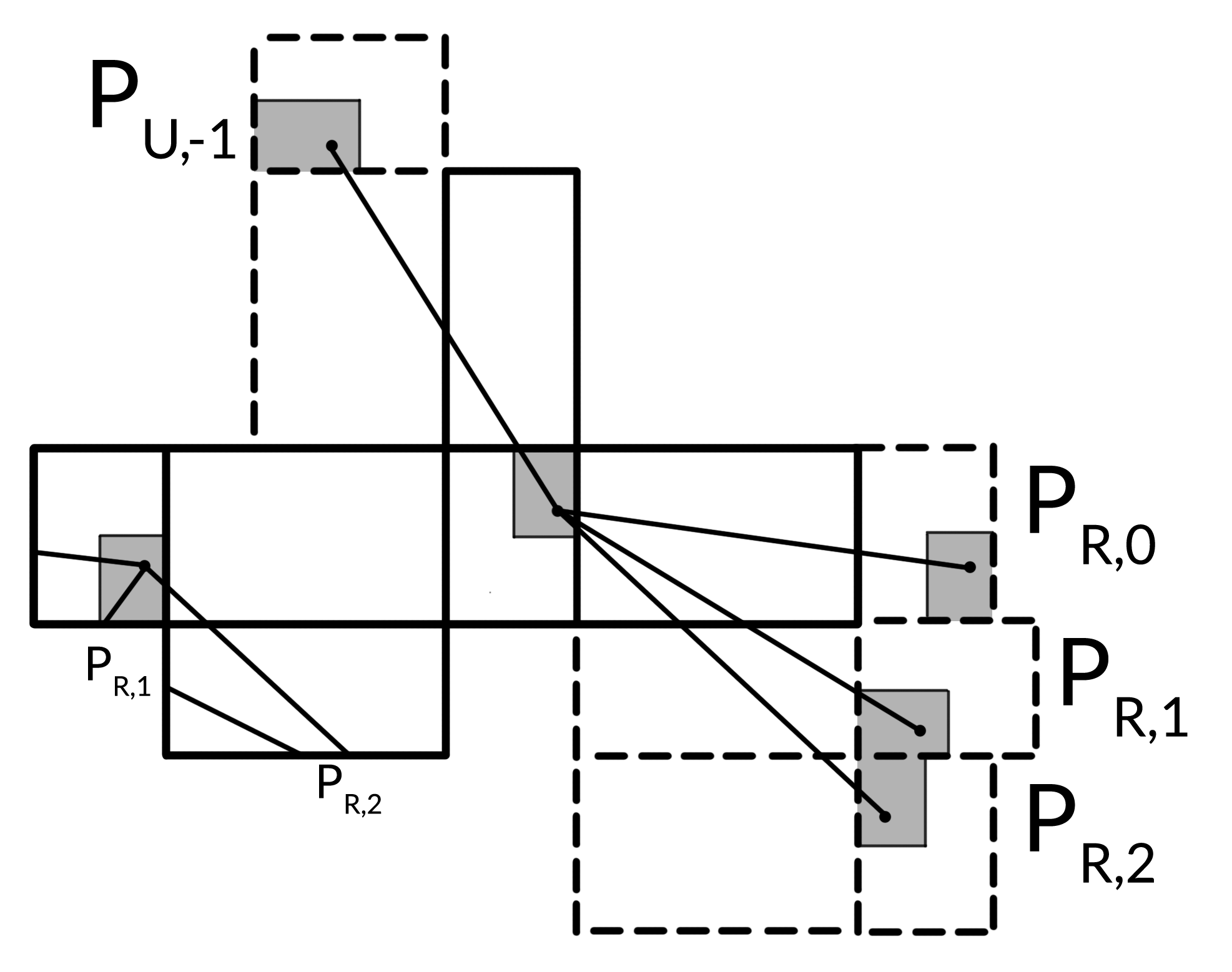
Figure 1: Four paths on flattenings of the box

Proposition 1

Paths with $|j|\geq 3$ can not be shortest.

Proof: First assume $j=3$. We will prove this by contradiction. Assume, for some $(a,b,x,y)$ and some $\ast\in\{R,U,L,D\}$, that $d_{\ast,3}<d_{\ast,-1}$. Note that $p_{\ast,3}$ and $p_{\ast,-1}$ cross the same initial side faces and same final side faces. Consider a new path that is identical to $p_{\ast,3}$ on the top and bottom faces. Along the two side faces that $p_{\ast,-1}$ crosses, complete the new path by connecting the points where $p_{\ast,3}$ meets the edges of the top and bottom faces with the shortest possible path (it will be a line segment when those two side faces are flattened). Note that the length of the new path is at least $d_{\ast,-1}$, since it crosses the same faces as $p_{\ast,-1}$.

The path $p_{\ast,3}$ and the new path are identical except on the sides faces. On flattened side faces, $p_{\ast,3}$ and the new path are each the hypotenuse of a right triangle with one side of length $b$ (the height of each side face). For $p_{\ast,3}$, the other side of the right triangle has length greater than $1+a$, which is the width of the second and third of the four side faces it crosses. On the new path, the other side of the right triangle has length less than $1+a$, which is the width of the two side faces it crosses. So the new path has length less than $d_{\ast,3}$ and at least $d_{\ast,-1}$; this is a contradiction. For the argument for $j=-3$, just flip the signs in the subscripts.

The cases where $|j|\geq 4$, where paths cross at least five side faces, are obvious.   QED

Note that if we started at the point $(x,y)=(\frac{a}{2},\frac{1}{2})$ and traveled along the edge not bordering ${\mathcal{F}}$, or had a path that eventually traveled along this edge or any edge parallel to it, then this would be a degenerate form of more than one of the paths given and thus would be considered in our analysis.

By cutting along edges, the 3, 4 or 5 faces that a path crosses can be flattened out onto a plane, which is the easiest way to determine the length of the corresponding paths.

Note that a line segment path from one point to its opposite can leave and reenter a flattening. We do not need to worry about this case because it leaves and reenters on what is the same edge of the box. By gluing those edges back together and possibly perturbing the path, we get a different and shorter path.

The referee pointed out that the map that reflects points across the origin (the antipodal map) interchanges pairs of paths. The pairs are $\{p_{\ast,2},p_{\ast,-2}\}$ (for each $\ast$), $\{p_{R,1},p_{U,-1}\}$, $\{p_{U,1},p_{L,-1}\}$, $\{p_{L,1},p_{D,-1}\}$, $\{p_{D,1},p_{R,-1}\}$, $\{p_{R,0},p_{L,0}\}$, and $\{p_{U,0},p_{D,0}\}$. This is illustrated in Figure 1 for $p_{R,1}$ and $p_{U,-1}$. The length of each path in a pair is the same. So to minimize distance, it suffices to consider one path in each pair. We choose $p_{\ast,2}$, $p_{R,1}$, $p_{U,1}$, $p_{L,1}$, $p_{D,1}$, $p_{R,0}$, and $p_{U,0}$. In Table 1, for a point $(x,y)\in{\mathcal{F}}$, we give the coordinates of the opposite point, given the obvious flattening for each of the 10 paths (this is illustrated in Figure 1 for four of the paths), and $d_{\ast,j}$, the square of the distance between them. In the table we let $a_{1}=\frac{a+1}{2}$.

path	point opposite of $(x,y)$	$d_{*,j}=$ squared distance to $(x,y)$
$p_{R,0}$	$(x+a+b,-y)$	$4y^{2}+a^{2}+2ba+b^{2}$
$p_{R,1}$	$(-y+a_{1}+b,-x-a_{1})$	$2x^{2}+4xy+2y^{2}-2bx-2by+\frac{1}{2}a^{2}+(b+1)a+b^{2}+b+\frac{1}{2}$
$p_{R,2}$	$(-x+a+b,y-a-1)$	$4x^{2}+(-4a-4b)x+2a^{2}+(2b+2)a+b^{2}+1$
$p_{U,0}$	$(-x,y+b+1)$	$4x^{2}+b^{2}+2b+1$
$p_{U,1}$	$(y+a_{1},x+a_{1}+b)$	$2x^{2}-4xy+2y^{2}+2bx-2by+\frac{1}{2}a^{2}+(b+1)a+b^{2}+b+\frac{1}{2}$
$p_{U,2}$	$(x+a+1,-y+b+1)$	$4y^{2}+(-4b-4)y+a^{2}+2a+b^{2}+2b+2$
$p_{L,1}$	$(-y-a_{1}-b,-x+a_{1})$	$2x^{2}+4xy+2y^{2}+2bx+2by+\frac{1}{2}a^{2}+(b+1)a+b^{2}+b+\frac{1}{2}$
$p_{L,2}$	$(-x-a-b,y+a+1)$	$4x^{2}+(4a+4b)x+2a^{2}+(2b+2)a+b^{2}+1$
$p_{D,1}$	$(y-a_{1},x-a_{1}-b)$	$2x^{2}-4xy+2y^{2}-2bx+2by+\frac{1}{2}a^{2}+(b+1)a+b^{2}+b+\frac{1}{2}$
$p_{D,2}$	$(x-a-1,-y-b-1)$	$4y^{2}+(4b+4)y+a^{2}+2a+b^{2}+2b+2$

Table 1: The 10 distance functions (note $a_{1}=\frac{a+1}{2}$)

By inspection we see that $d_{R,2}\leq d_{L,2}$, $d_{U,2}\leq d_{D,2}$ and $d_{D,1}\leq d_{L,1}$. Since we are minimizing distance, we no longer consider $d_{L,2}$, $d_{D,2}$ or $d_{L,1}$. So it suffices to consider the seven distance functions $d_{R,0}$, $d_{R,1}$, $d_{R,2}$, $d_{U,0}$, $d_{U,1}$, $d_{U,2}$ and $d_{D,1}$.

Proposition 2

For all $P=(a,b,x,y)$ with $0<a\leq 1$, $0<b$, $0\leq x\leq\frac{a}{2}$, $0\leq y\leq\frac{1}{2}$ we have $d_{D,1}(P)\geq{\rm min}\{d_{R,0}(P),d_{R,1}(P),d_{U,1}(P)\}$.

Proof: We have $d_{D,1}-d_{U,1}=4b(y-x)$. So for $y\geq x$ we see $d_{U,1}\leq d_{D,1}$. We have $d_{D,1}-d_{R,1}=4y(b-2x)$. So for $b\geq a$ we see $b\geq a\geq 2x$ and $d_{R,1}\leq d_{D,1}$. Let ${\mathcal{R}}$ be the subset $b<a$ of the $ab$-plank and ${\mathcal{F}}^{\prime}$ be the region $y<x$ in the fundamental region associated to a given $(a,b)\in{\mathcal{R}}$. For $d_{D,1}$ to be smallest (i.e. uniquely minimal) among the seven distance functions, we need $(a,b)\in{\mathcal{R}}$ and $(x,y)\in{\mathcal{F}}^{\prime}$.

We now show that for all $(a,b,x,y)$ with $(a,b)\in{\mathcal{R}}$ and $(x,y)\in{\mathcal{F}}^{\prime}$ we have $d_{D,1}(a,b,x,y)\geq d_{R,0}(a,b,x,y)$. Note that for $(a,b,x,y)=(.8,.7,.3,.2)$ we have $d_{D,1}>d_{R,0}$. Since $d_{D,1}-d_{R,0}$ is a polynomial function, we can use a continuity argument to show that if there is an $(a,b)\in{\mathcal{R}}$ for which there is an $(x,y)\in{\mathcal{F}}^{\prime}$ such that $d_{D_{1}}(a,b,x,y)<d_{R,0}(a,b,x,y)$ then the hyperbola $d_{D,1}=d_{R,0}$ (for the given $(a,b)$) must pass through the interior of ${\mathcal{F}}^{\prime}$, and so intersect the boundary of ${\mathcal{F}}^{\prime}$ in two different points. We will show that this does not occur.

Let $\bar{{\mathcal{F}}^{\prime}}$ denote the closure of ${\mathcal{F}}^{\prime}$ in ${\mathcal{F}}$. The boundary of ${\mathcal{F}}^{\prime}$ (and of $\bar{{\mathcal{F}}^{\prime}}$) consists of $y=0$ and $y=x$ with $0\leq x\leq\frac{a}{2}$, and $x=\frac{a}{2}$ with $0\leq y\leq\frac{a}{2}$. The hyperbola $d_{D,1}=d_{R,0}$ meets $y=0$ where $2x=b\pm\sqrt{(a+b-1)^{2}-2}$. Since $0<b<a\leq 1$ we have $-1<a+b-1<1$. So $(a+b-1)^{2}-2<-1$. Thus the hyperbola does not meet $y=0$ for $(a,b)\in{\mathcal{R}}$. The hyperbola $d_{D,1}=d_{R,0}$ meets $y=x$ where $x^{2}=\frac{1}{8}(-a^{2}-2ab+2a+2b+1)$. Since $a\leq 1$ we have $3a^{2}+2ab\leq 3a+2b\leq 2a+2b+1$. So $2a^{2}\leq-a^{2}-2ab+2a+2b+1$ and $\frac{a^{2}}{4}\leq x^{2}$. Since $(x,y)\in\bar{{\mathcal{F}}^{\prime}}$ we have $x^{2}\leq\frac{a^{2}}{4}$. So the hyperbola $d_{D,1}=d_{R,0}$ can only meet $y=x$ in $\bar{{\mathcal{F}}^{\prime}}$ at $(x,y)=(\frac{a}{2},\frac{a}{2})$. The hyperbola $d_{D,1}=d_{R,0}$ meets $x=\frac{a}{2}$ where $2y=b-a\pm\sqrt{a^{2}-6ab+b^{2}+2a+2b+1}$. Since $b<a$ in ${\mathcal{R}}$ and $y\geq 0$, the hyperbola $d_{D,1}=d_{R,0}$ meets $x=\frac{a}{2}$ where $2y=b-a+\sqrt{a^{2}-6ab+b^{2}+2a+2b+1}$. From above $3a^{2}+2ab\leq 2a+2b+1$; so $(2a-b)^{2}\leq a^{2}-6ab+b^{2}+2a+2b+1$. We have $2a-b\leq\sqrt{a^{2}-6ab+b^{2}+2a+2b+1}$. Thus $a\leq b-a+\sqrt{a^{2}-6ab+b^{2}+2a+2b+1}$. So $a\leq 2y$. In $\bar{{\mathcal{F}}^{\prime}}$ we have $y\leq x\leq\frac{a}{2}$. So the hyperbola $d_{D,1}=d_{R,0}$ can only meet $x=\frac{a}{2}$ in $\bar{{\mathcal{F}}^{\prime}}$ at $(x,y)=(\frac{a}{2},\frac{a}{2})$. So the hyperbola can not meet the boundary of ${\mathcal{F}}^{\prime}$ in two different points.   QED

So we see that the remaining six distance functions $d_{R,0}$, $d_{R,1}$, $d_{R,2}$, $d_{U,0}$, $d_{U,1}$ and $d_{U,2}$ are sufficient. We will see they are also necessary, in the sense that there are points $(a,b)$ in the $ab$-plank and points $(x,y)$ (in the associated fundamental regions) for which each of the six distance functions is strictly smaller than the other five.

For the remainder of this article, for a given $(a,b)$, we say that one of those six distance functions is smallest (respectively minimal), for a given $(x,y)$, if it is strictly smaller than (respectively smaller than or equal to) the other five distance functions. Note that the regions on which a distance function is smallest (respectively minimal) are open (respectively closed) subsets of ${\mathcal{F}}$.

3 The equivalence relation

For each $(a,b)$, there is an associated fundamental region ${\mathcal{F}}$. For each of the six distance functions, we can find the subset of ${\mathcal{F}}$ on which the distance function is smallest. Note that where two of these subsets border, two or more distance functions will have identical values. As suggested in the introduction, we use topology to define an equivalence relation on points $(a,b)$, in the $ab$-plank, for which the corresponding partitionings of their fundamental regions “look essentially the same”. We do not technically have a partition since the subsets on which each distance functions are minimal can overlap on boundary curves.

Let $d_{\alpha}$ denote an element of the set $\{d_{R,0},d_{R,1},d_{R,2},d_{U,0},d_{U,1},d_{U,2}\}$. For each fundamental region ${\mathcal{F}}$ we call a connected component of the subset on which $d_{\alpha}$ is smallest a $d_{\alpha}$-region. For a given fundamental region ${\mathcal{F}}$, let $S$ be the union of the borders of the $d_{\alpha}$-regions (including the four sides of ${\mathcal{F}}$). We use $\prod_{0}({\mathcal{F}}\setminus S)$ to denote the set of connected components of ${\mathcal{F}}\setminus S$; each is a $d_{\alpha}$-region. Let $f:\prod_{0}({\mathcal{F}}\setminus S)\rightarrow\{d_{R,0},d_{R,1},d_{R,2},d_{U,0},d_{U,1},d_{U,2}\}$ be the function that sends a $d_{\alpha}$-region to $d_{\alpha}$. Let $Q$ and $R$ be points in the $ab$-plank; we use $Q$ and $R$ as subscripts to indicate to which point a particular notation is associated. We say that $Q$ is equivalent to $R$ if and only if there is a homeomorphism $\iota:{\mathcal{F}}_{Q}{\rightarrow}{\mathcal{F}}_{R}$ with the following properties: i) $\iota|_{S_{Q}}$ induces a homeomorphism of $S_{Q}$ and $S_{R}$, ii) $\iota$ sends $(0,0)$, $(0,\frac{1}{2})$, $(\frac{a_{Q}}{2},0)$ and $(\frac{a_{Q}}{2},\frac{1}{2})$ to $(0,0)$, $(0,\frac{1}{2})$, $(\frac{a_{R}}{2},0)$ and $(\frac{a_{R}}{2},\frac{1}{2})$, respectively, and iii) we have $f_{R}\circ\iota|_{\prod_{0}({\mathcal{F}}_{Q}\setminus S_{Q})}=f_{Q}$ (where $\iota|_{\prod_{0}({\mathcal{F}}_{Q}\setminus S_{Q})}$ is the obvious induced map). Our goal is to find the equivalence classes for this relation. We call a pair $({\mathcal{F}},f)$ a labeled ${\mathcal{F}}$. For each equivalence class, we will also describe the associated labeled ${\mathcal{F}}$’s.

4 The equivalence classes

Now we want to partition the $ab$-plank by the equivalence classes defined in Section 3. We will prove that there are 47 of them, some having area, some having length and two are single points. We use reverse lexicographical order on $(a,b)$ to order the equivalence classes. In Table 2 we define the 47 equivalence classes, give the dimension of each and give a set of equalities and inequalities that define the subset of the $ab$-plank that is the given equivalence class. In Table 2, $a^{\prime}$ is the root of $a^{4}-2a^{3}+7a^{2}-6a+1$ near $0.780$, $a^{\prime\prime}$ is the root of $8a^{5}+12a^{4}+a^{3}-10a^{2}-6a-1$ near $0.927$, $b^{\prime}$ is the root of $4b^{3}+3b-6$ near $0.929$, $b^{\prime\prime}$ is the root of $6b^{7}-7b^{6}-12b^{5}+7b^{4}+8b^{3}-b^{2}-2b-1$ near 1.72, and $b^{\prime\prime\prime}$ is the root of $3b^{4}-10b^{3}+11b^{2}-6b+1$ near $1.92$.

All of the curves listed in Table 2 are lines or conic sections, and so are easy to graph, except the two quartics $(b^{2}+1)a^{2}+2b^{3}a-2b^{3}-b^{2}=0$ and $(2b-2)a^{3}+(b^{2}-1)a^{2}-b^{2}=0$. In addition, for the proof of Proposition 16, we will need to graph $(b^{2}+1)a^{2}+2a-b^{2}-2b=0$. The software Magma (see [Ma]) shows that each is a singular curve of genus 1 and finds a real birational map to the projective closures of the non-singular curves $y^{2}=x^{3}+19x^{2}+120x+256$, $y^{2}=x^{3}+4x^{2}+256$ and $y^{2}=x^{3}+x^{2}+4$, respectively (see [Ha]). Since each cubic in $x$ has a single real root, each of those projective curves has a single real component. The images of each of these single real components in $ab$-space go off to infinity; so none of the quartics have a compact component. So we can trust graphing software to draw them without missing a small, compact component.

Equiv
class	dim	definition
1	2	$a+b-1\leq 0$, $a^{2}+2ab-2b\leq 0$
2	2	$a+b-1\leq 0$, $a^{2}+2ab-2b>0$
3	2	$a+b-1>0$, $a^{2}+2ab-2b>0$, $ab-2a+2b^{2}-3b+2>0$, $b<\frac{2}{3}$
4	1	$ab-2a+2b^{2}-3b+2=0$, $b<\frac{2}{3}$
5	2	[$ab-2a+2b^{2}-3b+2<0$, $b\leq\frac{2}{3}$, $a<1$] $\cup$
		[$(b^{2}+1)a^{2}+2b^{3}a-2b^{3}-b^{2}>0$, $a-b^{2}\geq 0$, $\frac{2}{3}<b<1$, $a<1$]
6	1	$a=1$, $0<b\leq 1$
7	2	$a+b-1>0$, $a^{2}+2ab-2b\leq 0$, $2b+a-2<0$
8	1	$2b+a-2=0$, $0<a\leq\frac{2}{3}$
9	2	$2b+a-2>0$, $a^{2}+(2b+2)a-4b\leq 0$, $a^{2}+(2b-2)a+3b^{2}-2b-1\leq 0$
10	2	$a^{2}+(2b+2)a-4b>0$, $(b^{2}+1)a^{2}+2b^{3}a-2b^{3}-b^{2}<0$, $a^{2}+(2b-2)a+3b^{2}-2b-1\leq 0$
11	1	$(b^{2}+1)a^{2}+2b^{3}a-2b^{3}-b^{2}=0$, $\frac{2}{3}<a\leq a^{\prime}$
12	2	$a^{2}+(2b+2)a-4b>0$, $(b^{2}+1)a^{2}+2b^{3}a-2b^{3}-b^{2}\leq 0$,
		$a^{2}+(2b-2)a+3b^{2}-2b-1>0$
13	2	$(b^{2}+1)a^{2}+2b^{3}a-2b^{3}-b^{2}>0$, $a^{2}+(2b+2)a-4b>0$, $(\sqrt{2}+1)a-b-1<0$, $a^{\prime}<a<2\sqrt{2}-2$
14	1	$(\sqrt{2}+1)a-b-1=0$, $a^{\prime}<a<2\sqrt{2}-2$
15	2	$a-b^{2}<0$, $(\sqrt{2}+1)a-b-1>0$, $b<1$
16	2	$a^{2}+(2b+2)a-4b\leq 0$, $(b^{2}+1)a^{2}+2b^{3}a-2b^{3}-b^{2}\leq 0$,
		$a^{2}+(2b-2)a+3b^{2}-2b-1>0$, $b<1$
17	2	$(b^{2}+1)a^{2}+2b^{3}a-2b^{3}-b^{2}>0$, $b^{\prime}<b<1$, $a^{2}+(2b+2)a-4b\leq 0$
18	1	$b=1$, $0<a\leq\frac{-1+\sqrt{7}}{2}$
19	1	$b=1$, $\frac{-1+\sqrt{7}}{2}<a<2\sqrt{2}-2$
20	0	$(a,b)=(2\sqrt{2}-2,1)$
21	1	$b=1$, $2\sqrt{2}-2<a<1$
22	2	$a-b+1\leq 0$, $2ab-2a-1<0$
23	2	$a-b+1>0$, $2a^{2}+(-3b+1)a+2b^{2}-2b>0$,
		$2ab-2a-1<0$, $(b^{2}+1)a^{2}+2b^{3}a-2b^{3}-b^{2}\leq 0$, $b>1$
24	2	$2a^{2}+(-3b+1)a+2b^{2}-2b\leq 0$, $a-2b+2<0$, $(b^{2}+1)a^{2}+2b^{3}a-2b^{3}-b^{2}\leq 0$
25	2	$b>1$, $a-2b+2\geq 0$, $(b^{2}+1)a^{2}+2b^{3}a-2b^{3}-b^{2}\leq 0$
26	2	$b>1$, $(b^{2}+1)a^{2}+2b^{3}a-2b^{3}-b^{2}>0$, $a^{2}+(2b+2)a-4b<0$, $a-2b+2\geq 0$
27	1	$a^{2}+(2b+2)a-4b=0$, $2\sqrt{2}-2<a<1$
28	2	$a<1$, $1<b$, $a^{2}+(2b+2)a-4b>0$
29	1	$a=1$, $1<b<\frac{3}{2}$
30	2	$a-2b+2<0$, $(b^{2}+1)a^{2}+2b^{3}a-2b^{3}-b^{2}>0$, $2a^{2}+(-3b+1)a+2b^{2}-2b\leq 0$
31	2	$2a^{2}+(-3b+1)a+2b^{2}-2b>0$, $(b^{2}+1)a^{2}+2b^{3}a-2b^{3}-b^{2}>0$, $2ab-2a-1<0$, $b>1$
32	0	$(a,b)=(1,\frac{3}{2})$
33	1	$2ab-2a-1=0$, $a^{\prime\prime}<a<1$
34	2	$2ab-2a-1>0$, $(b^{2}+1)a^{2}+2b^{3}a-2b^{3}-b^{2}>0$, $(2b-2)a^{3}+(b^{2}-1)a^{2}-b^{2}<0$
35	1	$(2b-2)a^{3}+(b^{2}-1)a^{2}-b^{2}=0$, $\frac{3}{2}<b<b^{\prime\prime}$
36	2	$(2b-2)a^{3}+(b^{2}-1)a^{2}-b^{2}>0$, $(b^{2}+1)a^{2}+2b^{3}a-2b^{3}-b^{2}>0$, $a-b+1>0$, $a<1$
37	1	$a=1$, $\frac{3}{2}<b<2$
38	1	$2ab-2a-1=0$, $\frac{1}{\sqrt{2}}<a\leq a^{\prime\prime}$
39	2	$2ab-2a-1>0$, $(b^{2}+1)a^{2}+2b^{3}a-2b^{3}-b^{2}\leq 0$,
		$(2b-2)a^{3}+(b^{2}-1)a^{2}-b^{2}<0$, $a-b+1>0$
40	1	$2ab-2a-1=0$, $1+\frac{1}{\sqrt{2}}\leq b$
41	2	$2ab-2a-1>0$, $a-b+1\leq 0$, $(2b-2)a^{3}+(b^{2}-1)a^{2}-b^{2}<0$
42	1	$(2b-2)a^{3}+(b^{2}-1)a^{2}-b^{2}=0$, $b^{\prime\prime}\leq b<b^{\prime\prime\prime}$
43	2	$(2b-2)a^{3}+(b^{2}-1)a^{2}-b^{2}>0$, $(b^{2}+1)a^{2}+2b^{3}a-2b^{3}-b^{2}\leq 0$, $a-b+1>0$
44	1	$(2b-2)a^{3}+(b^{2}-1)a^{2}-b^{2}=0$, $b^{\prime\prime\prime}\leq b$
45	2	$(2b-2)a^{3}+(b^{2}-1)a^{2}-b^{2}>0$, $(b^{2}+1)a^{2}+2b^{3}a-2b^{3}-b^{2}\leq 0$, $a-b+1\leq 0$
46	2	$(b^{2}+1)a^{2}+2b^{3}a-2b^{3}-b^{2}>0$, $a-b+1\leq 0$, $a<1$
47	1	$a=1$, $2\leq b$

Table 2: The 47 equivalence classes

In Figure 2, we show the partition of the $ab$-plank into the 47 equivalence classes. For 2-dimensional equivalence classes, we use arrows to denote which boundaries are part of the equivalence class. It is difficult to include equivalence classes 10 - 14, 17, 19, 20 and 31 - 33 in our figure as they are small. For example, four of the 2-dimensional classes, 10, 12, 13 and 17, have areas that are approximately 0.00075, 0.000062, 0.000035 and 0.00018, respectively.

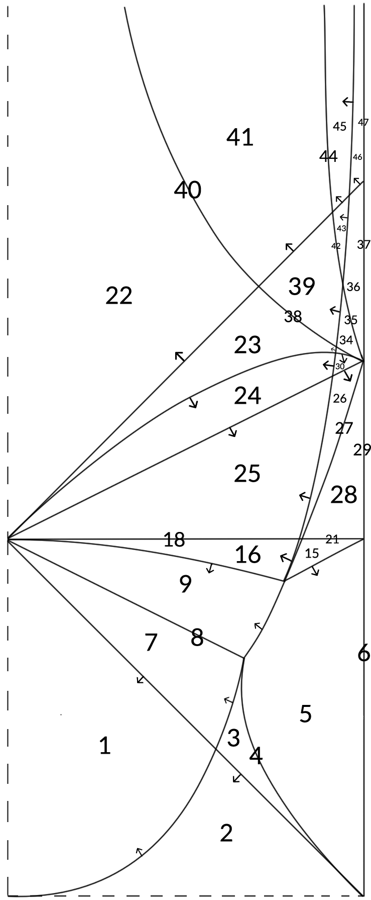
Figure 2: The 47 equivalence classes in the $ab$-plank

In Figures 3 and 4, we present a labeled ${\mathcal{F}}$ for each of the 47 equivalence classes, that is homeomorphic (with the three properties listed at the end of Section 3) to the labeled ${\mathcal{F}}$ for each $(a,b)$ in the equivalence class. For simplicity, we give only the subscripts of the labeling and omit the $d$’s and commas.

A priori, it seems surprising in equivalence class 13 that there are disjoint subsets of ${\mathcal{F}}$ on which $d_{U,0}$ is smallest. We will see, in Section 5, for 13 of the pairs $d_{\alpha},d_{\beta}$, that $d_{\alpha}=d_{\beta}$ is a hyperbola in the $xy$-plane. So, without loss of generality, there are two disjoint components of the $xy$-plane on which $d_{\alpha}<d_{\beta}$. Perhaps we should be surprised that there is a unique equivalence class in which this occurs in ${\mathcal{F}}$.

We also note, when passing from equivalence class 5 to 15, a subset arises in the interior of ${\mathcal{F}}$ in which $d_{R,1}$ is smallest. Such subsets also arise in the interior of the $1\times a$ face, though on a border of ${\mathcal{F}}$: when crossing $(b^{2}+1)a^{2}+2b^{3}a-2b^{3}-b^{2}=0$ for $a>a^{\prime}$, from left to right, and when crossing $a^{2}+(2b-2)a+3b^{2}-2b-1=0$ for $a<a^{\prime}$, from below to above, interior subsets arise in which $d_{U,0}$ and $d_{R,1}$, respectively, are smallest.

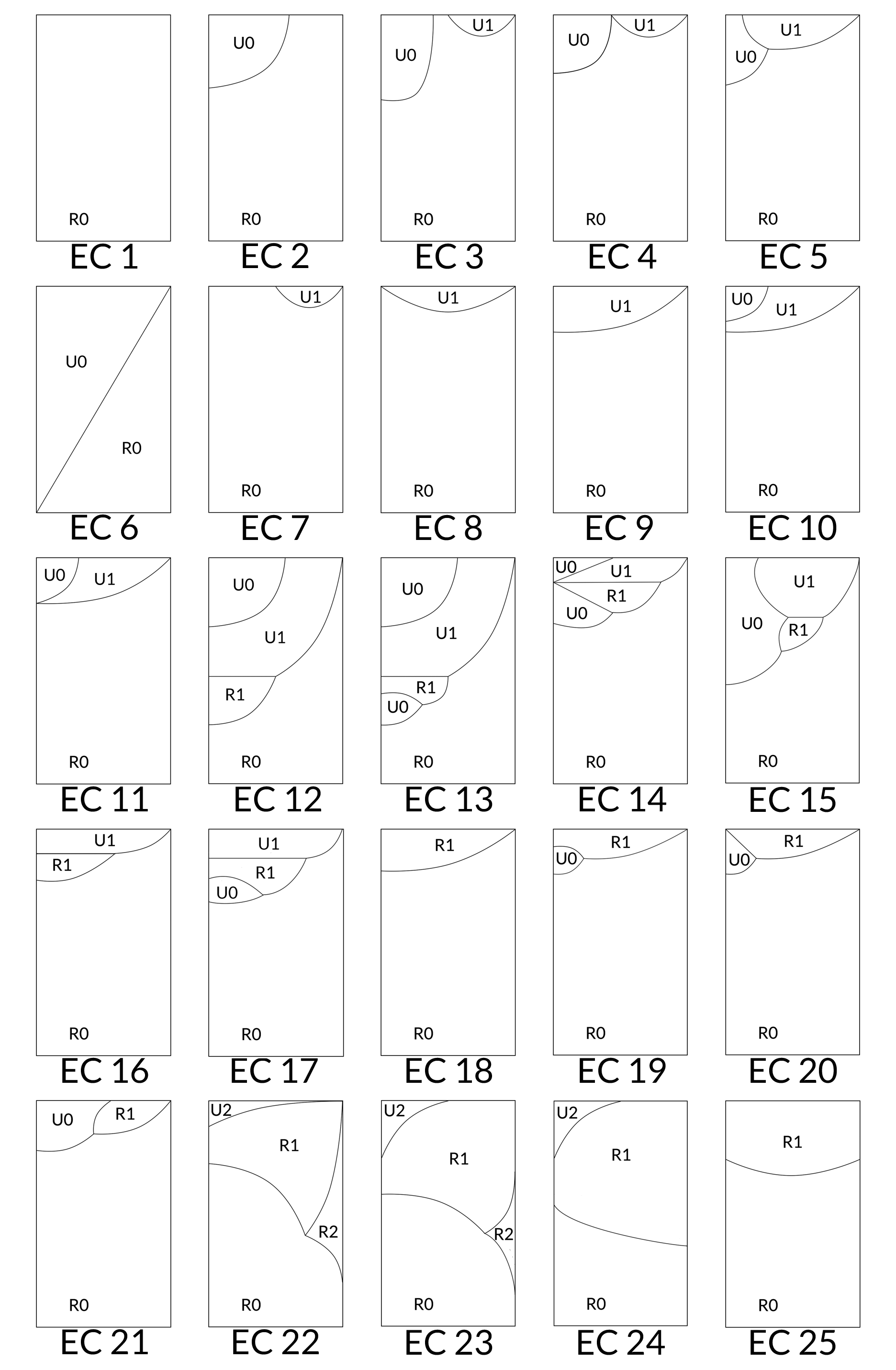
Figure 3: Labeled ${\mathcal{F}}$’s for Equivalence Classes 1 - 25

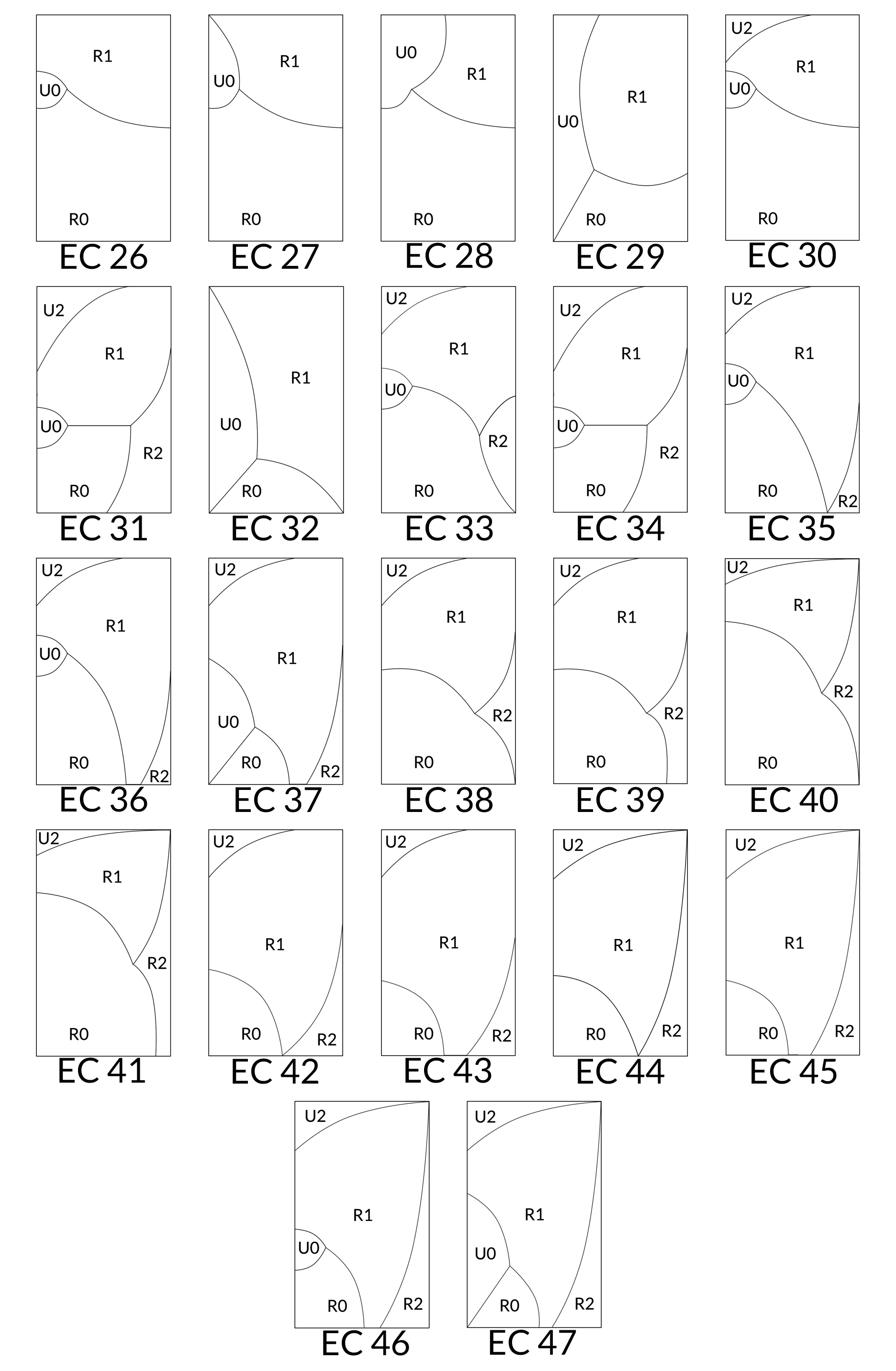
Figure 4: Labeled ${\mathcal{F}}$’s for Equivalence Classes 26 - 47

5 Distance functions in pairs

It is useful for understanding where the equivalence classes change in the $ab$-plank to equate the six distance functions, two at a time.

Lemma 1

Fix two distinct distance functions $d_{\alpha}$, $d_{\beta}$, from the six of concern. Let ${\mathcal{P}}$ be a path in the $ab$-plank. For each point in the path there is a labeled ${\mathcal{F}}$, considering only $d_{\alpha}$ and $d_{\beta}$. If the equivalence classes for these labeled ${\mathcal{F}}$’s are not all the same for the points on ${\mathcal{P}}$ then one of the following occurs at some point on ${\mathcal{P}}$: 1) $d_{\alpha}=d_{\beta}$ at a corner of ${\mathcal{F}}$, 2) $d_{\alpha}=d_{\beta}$ has a double intersection with a side of ${\mathcal{F}}$, 3) $d_{\alpha}=d_{\beta}$ consists of two line segments meeting in the interior of ${\mathcal{F}}$.

Note that a double intersection with a side of ${\mathcal{F}}$ is either a tangency, or the two lines of a degenerate hyperbola crossing a side, each transversally, at the same point. In iii), $d_{\alpha}=d_{\beta}$ is part of a degenerate hyperbola.

Proof: From Table 1, we have $d_{R,0}=d_{U,2}$ and $d_{R,2}=d_{U,0}$ given by $(2b+2)y+ab-a-b-1=0$ and $(2a+2b)x-a^{2}-ab-a+b=0$, respectively. If we fix $(a,b)$ in the $ab$-plank, then the extension of each of these equations to the entire $xy$-plane describes a line. The other ${6\choose 2}-2=13$ equations, obtained by setting two distinct distance functions to be equal, are of the form $\gamma x^{2}+\delta xy+\phi y^{2}+\ell_{1}(a,b)x+\ell_{2}(a,b)y+q(a,b)=0$, where $\gamma,\delta,\phi$ are constants (i.e. not depending on $a$ or $b$), the $\ell_{i}$ are polynomials of degree at most 1 and $q$ is a polynomial of degree at most 2. In all 13 cases we have $\delta^{2}-4\gamma\phi>0$. So if we fix $a$ and $b$, the resulting equation, when extended to the entire $xy$-plane, describes a hyperbola (possibly degenerate), which we sometimes refer to for clarity.

We fix a pair $d_{\alpha},d_{\beta}$. Assume we do not have equivalence of all points of ${\mathcal{P}}$. Since each $d_{\alpha}-d_{\beta}$ is a polynomial, a continuous parametrization of ${\mathcal{P}}$ induces a continuously parameterized family of lines or hyperbolas. Thus there is a point $Q\in{\mathcal{P}}$ with the property that for every $\epsilon>0$, sufficiently small, and for all points $R\neq Q$ on a fixed side of $Q$ in ${\mathcal{P}}$, with ${\rm dist}(Q,R)<\epsilon$, we have $Q$ and $R$ not equivalent.

Assume, for every $\epsilon>0$, sufficiently small, and for all points $R\neq Q$ on a fixed side of $Q$ in ${\mathcal{P}}$, with ${\rm dist}(Q,R)<\epsilon$, that there is a homeomorphism $\iota$ from ${\mathcal{F}}_{Q}$ to ${\mathcal{F}}_{R}$ satisfying conditions i) and ii) in the definition of the equivalence relation in Section 3. Let $\bar{\iota}$ denote the map induced from the set of open, connected components of ${\mathcal{F}}_{Q}\setminus S_{Q}$ to that of ${\mathcal{F}}_{R}\setminus S_{R}$ (recall $S$ is the union of $d_{\alpha}=d_{\beta}$ and the border of ${\mathcal{F}}$). Recall that we have a continuously parameterized family of lines or hyperbolas. Thus for all open, connected components $U$ of ${\mathcal{F}}_{Q}\setminus S_{Q}$, there is an $(x,y)\in U$ such that for all $\epsilon$, sufficiently small, we have $(x,y)\in\bar{\iota}(U)$ as well. We fix a continuous parametrization of ${\mathcal{P}}$ by the variable $t$. From above, there is no $t$ between $t_{Q}$ and $t_{R}$ such that $(d_{\alpha}-d_{\beta})(a(t),b(t),x,y)=0$. So by the Intermediate Value Theorem, $d_{\alpha}-d_{\beta}$ takes the same sign at $(a(t_{Q}),b(t_{Q}),x,y)$ and $(a(t_{R}),b(t_{R}),x,y)$. Thus condition iii) holds for $\iota$ as well.

We now prove the contrapositive of what remains to be proven. Assume that for $Q$, none of 1), 2) or 3) from this Lemma occur. There are 13 classes for ${\mathcal{F}}_{Q}$ and $S_{Q}$, up to rotation, reflection, and homeomorphism, preserving conditions i) and ii) of the equivalence relation; representatives are given in Figure 5. Informally, we see that small perturbations in each of the 13 representatives in Figure 5 do not lead to a change in equivalence class. In other words, we see for all $\epsilon>0$, sufficiently small, and all points $R\neq Q$ on a fixed side of $Q$ in ${\mathcal{P}}$, with ${\rm dist}(Q,R)<\epsilon$, that there is a homoeomorphism from ${\mathcal{F}}_{Q}$ to ${\mathcal{F}}_{R}$ satisfying conditions i) and ii) of the equivalence relation.   QED

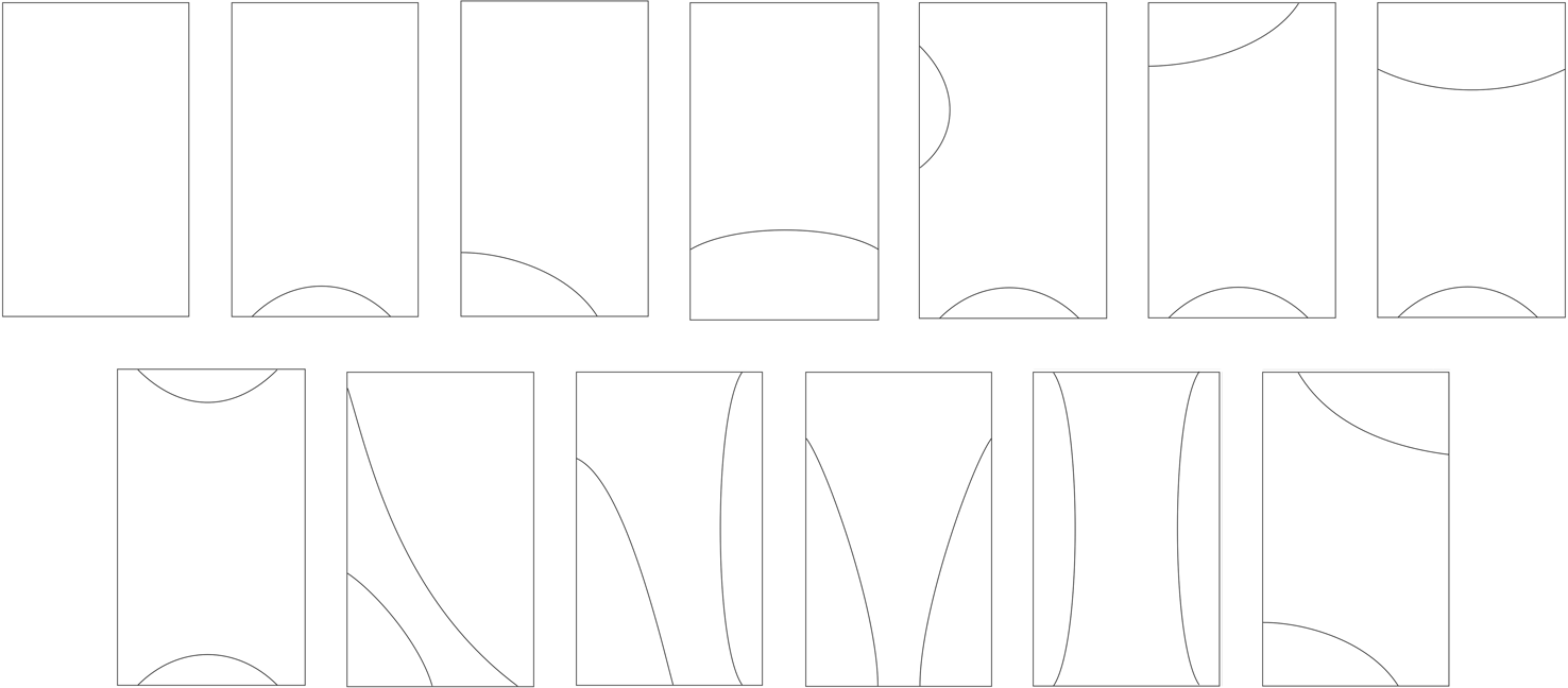
Figure 5: 13 Equivalence Classes for Lemma 1

For each pair $d_{\alpha},d_{\beta}$ we determine where, in the $(a,b)$ plank, each of the three conditions in Lemma 1 can occur (taking each corner and side of ${\mathcal{F}}$ into account). Most determine a curve in the $ab$-plank. We then break the $ab$-plank into equivalence classes for the labeled ${\mathcal{F}}$’s taking only $d_{\alpha}$ and $d_{\beta}$ into account. For nine of these pairs, this information is useful for determining the 47 equivalence classes and this is presented in Section 10. We do not attempt such computations for subsets of three or more of the distance functions simultaneously, because the possibilities lead to a combinatorial explosion.

6 Eliminating distance functions

For each of the six distance functions, we want to determine subsets of the $ab$-plank for which there is no $(x,y)$, in the associated fundamental region ${\mathcal{F}}$, for which the given distance function is smallest. We use the results from Section 10 to prove in Section 11 that certain distance functions can not be smallest on certain open subsets of the $ab$-plank. The interior of each 2-dimensional equivalence class is contained in one of these open subsets. As for 1- and 0-dimensional equivalence classes, by continuity, only those distance functions that are smallest in all of the bordering subsets can be smallest. In Table 3, we record this information by equivalence class.

Equivalence classes	functions that can be smallest
1	$d_{R,0}$
2, 6	$d_{R,0}$, $d_{U,0}$
3 - 5, 10, 11	$d_{R,0}$, $d_{U,0}$, $d_{U,1}$
7 - 9	$d_{R,0}$, $d_{U,1}$
12 - 15, 17	$d_{R,0}$, $d_{R,1}$, $d_{U,0}$, $d_{U,1}$
16	$d_{R,0}$, $d_{R,1}$, $d_{U,1}$
18, 25	$d_{R,0}$, $d_{R,1}$
19 - 21, 26 - 29, 32	$d_{R,0}$, $d_{R,1}$, $d_{U,0}$
22, 23, 38 - 45	$d_{R,0}$, $d_{R,1}$, $d_{R,2}$, $d_{U,2}$
24	$d_{R,0}$, $d_{R,1}$, $d_{U,2}$
30	$d_{R,0}$, $d_{R,1}$, $d_{U,0}$, $d_{U,2}$
31, 33 - 37, 46, 47	$d_{R,0}$, $d_{R,1}$, $d_{R,2}$, $d_{U,0}$, $d_{U,2}$

Table 3: Where distance functions can be smallest

7 Spontaneous generation of triple intersections

In this section, we describe the most interesting proof technique we used (in Sections 12 and 13) to determine the equivalence classes and associated labeled ${\mathcal{F}}$’s. Let $d_{\alpha}$, $d_{\beta}$, $d_{\gamma}$ be three distinct distance functions from the six of concern. If, for a given $(a,b)$, we have $(x,y)\in{\mathcal{F}}$ such that $d_{\alpha}(x,y)=d_{\beta}(x,y)=d_{\gamma}(x,y)$ then we call $(x,y)$ a triple intersection for $d_{\alpha},d_{\beta},d_{\gamma}$.

It will sometimes help to know, for a given three distance functions, that there is no triple intersection in the interior of ${\mathcal{F}}$. Let us start with a geometric example of what we call a spontaneous generation of a triple intersection. Then we give a rigorous definition and a description of how to find them. As an example, let $d_{\alpha},d_{\beta},d_{\gamma}$ denote three distinct distance functions. Assume for all $(a,b)$ in some open subset $U$ of the $ab$-plank, that $d_{\alpha}=d_{\beta}$ is a single arc, concave up, with lowest point $(\frac{a}{4},y_{L})$ (with $0<y_{L}<\frac{1}{2}$ and $y_{L}$ depending on $(a,b)$); $d_{\alpha}$ is smaller above the arc and $d_{\beta}$ below. Assume for all $(a,b)$ in $U$, that $d_{\beta}=d_{\gamma}$ is a single arc, concave down, with highest point $(\frac{a}{4},y_{U})$ (with $0<y_{U}<\frac{1}{2}$ and $y_{U}$ depending on $(a,b)$); $d_{\beta}$ is smaller above the arc and $d_{\gamma}$ below. Assume that there is a path in $U$ from $(a_{0},b_{0})$ to $(a_{1},b_{1})$ (distinct points) and on all points of the path except $(a_{0},b_{0})$ we have $y_{U}<y_{L}$ and at $(a_{0},b_{0})$ we have $y_{U}=y_{L}$. Then at $(a_{0},b_{0})$ we have the spontaneous generation of a triple intersection for $d_{\alpha}$, $d_{\beta}$, $d_{\gamma}$ at $(\frac{a}{4},y_{L})$. Note that if we consider only $d_{\alpha}$, $d_{\beta}$ and $d_{\gamma}$, then the labeled ${\mathcal{F}}$ at $(a_{0},b_{0})$ is not equivalent to those for other points on the path.

Now we give a rigorous definition. Let $d_{\alpha},d_{\beta},d_{\gamma}$ denote three distinct distance functions from the six of concern. Assume there is a given $(a_{0},b_{0})$ for which $d_{\alpha}=d_{\beta}=d_{\gamma}$ at some point $(x_{0},y_{0})$ in the interior of ${\mathcal{F}}$. Assume also that there is no neighborhood of $(a_{0},b_{0})$ inside which, for every point $(a,b)$ in the neighborhood we have $d_{\alpha}=d_{\beta}=d_{\gamma}$ at some point $(x,y)$ in the interior of ${\mathcal{F}}$. Then we define $(a_{0},b_{0},x_{0},y_{0})$ to be a spontaneous generation of a triple intersection for $d_{\alpha},d_{\beta},d_{\gamma}$.

To find the set of $(a,b)$’s at which they occur, we can take the resultant of $d_{\alpha}-d_{\beta}$ and $d_{\alpha}-d_{\gamma}$ with respect to $y$. This defines a surface (with possibly more than one component) in $abx$-space. We then take the projection of this surface onto the $ab$-plank. If $(a_{0},b_{0},x_{0},y_{0})$ is a spontaneous generation, then the projection of $(a_{0},b_{0},x_{0})$ on the $ab$-plank will be on the boundary of the projection of a neighborhood of $(a_{0},b_{0},x_{0})$ in the surface. At such a point $(a_{0},b_{0},x_{0})$, a normal vector to the surface will be parallel to the $ab$-plank. So we can find conditions on $a$ and $b$ for such points by taking the resultant, with respect to $x$, of a polynomial defining the surface, with its partial derivative with respect to $x$. The following theorem will be used in two of the proofs in Section 13 determining the equivalence classes.

Theorem 1

For the triples $d_{R,1},d_{R,2},d_{U,2}$ and $d_{R,1},d_{R,2},d_{U,0}$ there is no spontaneous generation of a triple intersection.

Proof: For $d_{R,1},d_{R,2},d_{U,2}$ the points obtained at which a spontaneous generation of a triple intersection could occur are on $b(a+1)(2a+2+b)=0$, which does not pass through the $ab$-plank. For $d_{R,1},d_{R,2},d_{U,0}$, after using a resultant to remove $y$ we get $4(a^{2}-2bx+ab+a-b-2ax)^{2}$. We then take the resultant, with respect to $x$, of $a^{2}-2bx+ab+a-b-2ax$ with its partial derivative with respect to $x$ to get $a+b$. But $a+b=0$ does not pass through the $ab$-plank.   QED

8 The equivalence class computations

For each subset of the $ab$-plank described in Table 2, we need only consider the distance functions listed in Table 3. Then, in the proofs in Sections 12 and 13, we show that changes in equivalence class can only occur along certain curves in the $ab$-plank. Nine of these equivalence class borders come from the $ab$-curves associated to the occurrences described in Lemma 1. Five of these borders are where three distance functions have a triple intersection on one of the four sides of ${\mathcal{F}}$. The curve $a-b^{2}=0$, for $a^{\prime}\leq a\leq 1$, is where $d_{R,0}=d_{R,1}=d_{U,0}=d_{U,1}$ at a point in ${\mathcal{F}}$ and the curve $(\sqrt{2}+1)a-b-1=0$, for $a^{\prime}\leq a\leq 2\sqrt{2}-2$, is where the hyperbolas $d_{R,1}=d_{U,0}$ and $d_{U,0}=d_{U,1}$ are both degenerate and the four lines making up those two hyperbolas all meet at one point on $x=0$ in ${\mathcal{F}}$.

In Sections 12 and 13, we also show that the labeled ${\mathcal{F}}$, for each $(a,b)$ in the given subset, is homeomorphic (with the three properties described in the definition of the equivalence relation in Section 3 of this article) to the one in Figure 3 or 4. As there is no such homeomorphism between any distinct pair of labeled ${\mathcal{F}}$’s in Figure 3 and 4, we then know that each of the 47 subsets is a distinct equivalence class.

9 Conclusion

In Dudeney’s problem we have a $12\times 12\times 30$ foot room. The spider is $1$ foot below the ceiling and half way between the sides of the room. In our notation we have $(a,b,x,y)=(1,\frac{5}{2},0,\frac{5}{12})$. This $(a,b)$ is in equivalence class 47 and this $(x,y)$ is on the border of the region where $d_{U,2}$ ($=d_{U,-2}$) is smallest. Indeed, on the path $p_{U,2}$, the spider must cross 5 sides for the shortest path to the fly. If, instead, the spider is $3$ feet below the ceiling of the same room then we have $(x,y)=(0,\frac{3}{12})$. This $(x,y)$ is on the border of where $d_{R,1}$ ($=d_{U,-1}$) is smallest and the shortest path to the fly opposite crosses 4 sides of the room. Lastly, if the spider is $5$ feet below the ceiling of the same room then we have $(x,y)=(0,\frac{1}{12})$. This $(x,y)$ is on the border of where $d_{U,0}$ is smallest and the obvious path, straight up, straight across the top and then straight down to the fly opposite is the shortest.

About the authors:

S.  Michael Miller was an undergraduate at the time of the writing of this article and is now pursuing his Ph.D. in Mathematics at the University of California, Los Angeles. Edward Schaefer is a professor, whose area is arithmetic geometry. He taught cryptography for two years at Mzuzu University in Malawi recently.

S.  Michael Miller

UCLA Mathematics Department, Box 951555 Los Angeles, CA 90095-1555. smmiller@g.ucla.edu

Edward F. Schaefer

Department of Mathematics and Computer Science, Santa Clara University, Santa Clara, CA 95053. eschaefer@scu.edu

APPENDIX

10 Distance functions in pairs

Lemma 2

Below $a+2b-2=0$, $d_{R,0}<d_{R,1}$. Between $a+2b-2=0$ and $b=1$, $d_{R,0}=d_{R,1}$ is a single arc, concave up, with positive slopes, meeting $x=0$ with $0<y<\frac{1}{2}$ and $y=\frac{1}{2}$ with $0<x<\frac{a}{2}$. To the left of the arc, $d_{R,1}$ is smaller and to the right, $d_{R,0}$ is.

On $b=1$, $d_{R,0}=d_{R,1}$ is a single arc with right endpoint $(\frac{a}{2},\frac{1}{2})$. The left endpoint is on $x=0$ with $0<y<\frac{1}{2}$. Above the arc, $d_{R,1}$ is smaller and below it, $d_{R,0}$ is.

For $b>1$, $d_{R,0}=d_{R,1}$ is a single arc. Its left endpoint is on $x=0$ with $0<y<\frac{1}{2}$. To the lower left of $(4b-2)a-2b-1=0$, the right endpoint is on $x=\frac{a}{2}$ with $0<y<\frac{1}{2}$. On $(4b-2)a-2b-1=0$, the right endpoint is $(\frac{a}{2},0)$. Above $(4b-2)a-2b-1=0$, the right endpoint is on $y=0$ with $0<x<\frac{a}{2}$. Above the arc, $d_{R,1}$ is smaller and below it, $d_{R,0}$ is.

Note $a+2b-2=0$ is where $d_{R,0}=d_{R,1}$ at $(0,\frac{1}{2})$.

Lemma 3

For $b<1$, $d_{R,0}<d_{R,2}$. For $b>1$, $d_{R,0}=d_{R,2}$ is a single arc with negative slopes (for $0<y$). Its upper endpoint is on $y=\frac{1}{2}$ with $0<x<\frac{a}{2}$. Below $2ab-2a-1=0$, the lower endpoint is on $x=\frac{a}{2}$ with $0<y<\frac{1}{2}$. On $2ab-2a-1=0$, the lower endpoint is $(\frac{a}{2},0)$. Above $2ab-2a-1=0$ , the lower endpoint is on $y=0$ with $0<x<\frac{a}{2}$. To the left of the arc, $d_{R,0}$ is smaller and to the right of it, $d_{R,2}$ is.

Note $b=1$ is where $d_{R,0}=d_{R,2}$ at $(\frac{a}{2},\frac{1}{2})$.

Lemma 4

On $a=1$, $d_{R,0}=d_{U,0}$ is a line segment connecting $(0,0)$ and $(\frac{1}{2},\frac{1}{2})$. Between $a=1$ and $a^{2}+2ab-2b=0$, $d_{R,0}=d_{U,0}$ is a single arc, concave up, with non-negative slopes, with left endpoint on $x=0$ with $0<y<\frac{1}{2}$ and right endpoint on $y=\frac{1}{2}$ with $0<x<\frac{a}{2}$. Above the arc, $d_{U,0}$ is smaller and below it, $d_{R,0}$ is. Above $a^{2}+2ab-2b=0$, $d_{R,0}<d_{U,0}$.

Note $a^{2}+2ab-2b=0$ is where $d_{R,0}=d_{U,0}$ at $(0,\frac{1}{2})$.

From Lemma 8, it suffices to consider $d_{U,1}$ for $b<1$.

Lemma 5

For all $(a,b)$, $d_{R,0}=d_{U,1}$ at $(\frac{a}{2},\frac{1}{2})$. Below $a+b-1=0$, $d_{R,0}=d_{U,1}$ meets ${\mathcal{F}}$ nowhere else and $d_{R,0}<d_{U,1}$ in the interior of ${\mathcal{F}}$. Between $a+b-1=0$ and $b=1$, $d_{R,0}=d_{U,1}$ is a single arc, concave up, with right endpoint at $(\frac{a}{2},\frac{1}{2})$. Between $a+b-1=0$ and $a+2b-2=0$, the left endpoint is on $y=\frac{1}{2}$ with $0<x<\frac{a}{2}$. On $a+2b-2=0$, the left endpoint is $(0,\frac{1}{2})$. Between $a+2b-2=0$ and $b=1$, the left endpoint is on $x=0$ with $0<y<\frac{1}{2}$. In each case, $d_{R,0}$ is smaller below the arc and $d_{U,1}$ above it.

Note $a+b-1=0$ is where $y=\frac{1}{2}$ is tangent to $d_{R,0}=d_{U,1}$ at $(\frac{a}{2},\frac{1}{2})$.

From Lemma 3, it suffices to consider $d_{R,2}$ for $b>1$.

Lemma 6

Assume $b>1$. For all $(a,b)$, $d_{R,1}=d_{R,2}$ at $(\frac{a}{2},\frac{1}{2})$. Below $2a-2b+1=0$, $d_{R,1}\neq d_{R,2}$ elsewhere and $d_{R,1}<d_{R,2}$ in the interior of ${\mathcal{F}}$. Above $2a-2b+1=0$, $d_{R,1}=d_{R,2}$ is the union of $(\frac{a}{2},\frac{1}{2})$ and a single arc with positive slopes. The left endpoint of the arc is on $x=0$ with $0<y<\frac{1}{2}$ for $(a,b)$ to the left of $3a^{2}+(2b+2)a-2b+1=0$, is $(0,0)$ for $3a^{2}+(2b+2)a-2b+1=0$, and is on $y=0$ with $0<x<\frac{a}{2}$ to the right of $3a^{2}+(2b+2)a-2b+1=0$. The right endpoint is on $x=\frac{a}{2}$ with $0<y<\frac{1}{2}$ below $a-b+1=0$ and at $(\frac{a}{2},\frac{1}{2})$ on or above $a-b+1=0$. Above the arc, $d_{R,1}$ is smaller and below it, $d_{R,2}$ is.

Note $a-b+1=0$ is where $x=\frac{a}{2}$ is tangent to $d_{R,1}=d_{R,2}$ at $(\frac{a}{2},\frac{1}{2})$.

Lemma 7

The hyperbola $d_{R,1}=d_{U,0}$ has asymptotes with slopes $-1\pm\sqrt{2}$.

On $(\sqrt{2}+1)a-b-1=0$ (which includes equivalence classes 14 and 20), the hyperbola $d_{R,1}=d_{U,0}$ is degenerate and the point of intersection of its two lines is on $x=0$. On equivalence class 14, $d_{R,1}=d_{U,0}$ is two line segments, each meeting $x=0$ at the same point with $0<y<\frac{1}{2}$. The other endpoints are on $y=0$ and $y=\frac{1}{2}$ with $0<x<\frac{a}{2}$. On equivalence class 20, $d_{R,1}=d_{U,0}$ is the line segment with endpoints $(0,\frac{1}{2})$ and $(\frac{\sqrt{2}-1}{2},0)$. In both cases, to the right of the segment or segments, $d_{R,1}$ is smaller and to the left, $d_{U,0}$ is.

To the right of $(\sqrt{2}+1)a-b-1=0$ (which includes equivalence class 15), only the component of the hyperbola $d_{R,1}=d_{U,0}$ to the right of the point of intersection of the asymptotes passes through ${\mathcal{F}}$ - one could say it is concave right. The lower endpoint of this arc is on $y=0$ with $0<x<\frac{a}{2}$ and its upper endpoint is on $x=\frac{a}{2}$ with $0<y\leq\frac{1}{2}$ or on $y=\frac{1}{2}$ with $0<x\leq\frac{a}{2}$. To the right of this arc, $d_{R,1}$ is smaller and to the left, $d_{U,0}$ is.

To the left of $(\sqrt{2}+1)a-b-1=0$ (which includes equivalence classes 12, 13 and 17), the two components of the hyperbola $d_{R,1}=d_{U,0}$ are above and below the point of intersection of their asymptotes and are hence concave up and down, respectively. In ${\mathcal{F}}$, when there are two arcs, $d_{R,1}$ is smaller between them and $d_{U,0}$ is smaller on the other sides of the arcs. When there is just the lower arc, $d_{R,1}$ is smaller above it and $d_{U,0}$ below.

Assume $(a,b)$ is to the right of $(b^{2}+1)a^{2}+2b^{3}a-2b^{3}-b^{2}=0$ with $b>1$. To the left of, and on, $a^{2}+(2b+2)a-4b=0$, $d_{R,1}=d_{U,0}$ is a single arc which is concave down and has negative slopes. The upper endpoint is on $x=0$ with $0<y<\frac{1}{2}$ to the left of $a^{2}+(2b+2)a-4b=0$ and is $(0,\frac{1}{2})$ on $a^{2}+(2b+2)a-4b=0$. The lower endpoint is on $y=0$ with $0<x<\frac{a}{2}$. To the right of the arc, $d_{R,1}$ is smaller and to the left, $d_{U,0}$ is. The only difference to the right of $a^{2}+(2b+2)a-4b=0$, is that the upper endpoint is on $y=\frac{1}{2}$ with $0<x<\frac{a}{2}$ and the arc is not necessarily concave down.

Note $(b^{2}+1)a^{2}+2b^{3}a-2b^{3}-b^{2}=0$ is where $d_{R,0}$, $d_{R,1}$, $d_{U,0}$ have a triple intersection on $x=0$ for $b\geq\frac{2}{3}$. Other aspects of where $d_{R,1}$ and $d_{U,0}$ are each smaller than the other will be described as needed.

Lemma 8

For $b\leq 1$, $d_{R,1}=d_{U,1}$ consists of the line segments $x=0$ and $y=\frac{b}{2}$. Below $y=\frac{b}{2}$, $d_{R,1}$ is smaller and above it, $d_{U,1}$ is. For $b>1$, $d_{R,1}=d_{U,1}$ is just $x=0$ and $d_{R,1}<d_{U,1}$ in the interior of ${\mathcal{F}}$.

Note $b=1$ is where a subset of $d_{R,1}=d_{U,1}$ coincides with $y=\frac{1}{2}$.

Lemma 9

For all $(a,b)$, $d_{R,1}=d_{U,2}$ at $(\frac{a}{2},\frac{1}{2})$. For $b\geq 1$ and on or below $a-2b+2=0$, $d_{R,1}=d_{U,2}$ at no other point or just $(0,\frac{1}{2})$ and $d_{R,1}<d_{U,2}$ in the interior of ${\mathcal{F}}$. Above $a-2b+2=0$, $d_{R,1}=d_{U,2}$ is the union of $(\frac{a}{2},\frac{1}{2})$ and a single arc with left endpoint on $x=0$ with $0<y<\frac{1}{2}$. Below $a-b+1=0$, the right endpoint is on $y=\frac{1}{2}$ with $0<x<\frac{a}{2}$ and on or above $a-b+1=0$ the right endpoint is $(\frac{a}{2},\frac{1}{2})$. Below the arc, $d_{R,1}$ is smaller and above it, $d_{U,2}$ is.

Note $d_{R,1}=d_{U,2}$ at $(0,\frac{1}{2})$ on $a-2b+2=0$ and is tangent to $y=\frac{1}{2}$ at $(\frac{a}{2},\frac{1}{2})$ on $a-b+1=0$.

From Lemma 8, it suffices to consider $d_{U,1}$ where $b<1$.

Lemma 10

Assume $b<1$. On $a=1$, $d_{U,0}=d_{U,1}$ does not pass through the interior of ${\mathcal{F}}$ and $d_{U,0}<d_{U,1}$ on the interior of ${\mathcal{F}}$.

Between $(\sqrt{2}+1)a-b-1=0$ and $a=1$ (which includes part of equivalence class 15), $d_{U,0}=d_{U,1}$ is a single arc. One endpoint is on $y=\frac{1}{2}$ with $0<x<\frac{a}{2}$ and the other is on $x=\frac{a}{2}$ with $0<y<\frac{1}{2}$. To the right of the arc, $d_{U,1}$ is smaller and to the left, $d_{U,0}$ is.

On $(\sqrt{2}+1)a-b-1=0$ (which includes equivalence class 14 and part of 15), $d_{U,0}=d_{U,1}$ consists of two line segments that meet $x=0$ with $0<y<\frac{1}{2}$ at the same point. The right endpoint of one line segment is on $y=\frac{1}{2}$ with $0<x<\frac{a}{2}$ and the right endpoint of the other is on $x=\frac{a}{2}$ with $0<y<\frac{1}{2}$. Between the line segments, $d_{U,1}$ is smaller and on the other sides of the segments, $d_{U,0}$ is.

Between $a^{2}+(2b+2)a-4b=0$ and $(\sqrt{2}+1)a-b-1=0$ (which includes equivalence classes 12 and 13 and part of 15), $d_{U,0}=d_{U,1}$ is two arcs. They have distinct left endpoints on $x=0$ with $0<y<\frac{1}{2}$. One has a right endpoint on $y=\frac{1}{2}$ with $0<x<\frac{a}{2}$. The other has a right endpoint on $x=\frac{a}{2}$ with $0<y<\frac{1}{2}$. Between the arcs, $d_{U,1}$ is smaller and on the other sides of the arcs, $d_{U,0}$ is.

Above $a^{2}+(2b+2)a-4b=0$ (which includes equivalence class 17), $d_{U,0}=d_{U,1}$ is a single arc, concave down, with endpoints on $x=0$ and $x=\frac{a}{2}$ and not meeting $y=0$ or $y=\frac{1}{2}$. Below the arc, $d_{U,0}$ is smaller and above it, $d_{U,1}$ is.

Note $a=1$ is where $d_{U,0}=d_{U,1}$ at $(\frac{a}{2},\frac{1}{2})$ and $a^{2}+(2b+2)a-4b=0$ is where $d_{U,0}=d_{U,1}$ at $(0,\frac{1}{2})$ for $b\leq 1$.

11 Eliminating distance functions

In this section, we fix a distance function and then describe subsets of the $ab$-plank for which there is no $(x,y)$, in the associated fundamental region ${\mathcal{F}}$, for which the given distance function is smallest. When that is the case, we will say that the given distance function is not smallest in that subset of the $ab$-plank.

Proposition 3

Let $(a,b)$ satisfy $a+2b-2>0$ and $b<1$ in the $ab$-plank. For all $(a,b)$ above the arc of the ellipse $a^{2}+(2b-2)a+3b^{2}-2b-1=0$, the labeled ${\mathcal{F}}$ for equivalence class 16 in Figure 3 shows where each of $d_{R,0},d_{R,1}$ and $d_{U,1}$ is smaller than the other two. The fundamental region for equivalence class 9 in Figure 3 shows this for $(a,b)$ on or below that arc.

Note $a^{2}+(2b-2)a+3b^{2}-2b-1=0$ is where $d_{R,0},d_{R,1},d_{U,1}$ have a triple intersection on $x=0$.

Proof: See Lemmas 2, 5 and 8 for where each of $d_{R,0}$, $d_{R,1}$ and $d_{U,1}$ is smaller than another, in pairs. If $d_{R,0}=d_{R,1}=d_{U,1}$ on $x=0$ then $a^{2}+(2b-2)a+3b^{2}-2b-1=0$. We can test sample $(a,b)$ above (respectively below) the arc of $a^{2}+(2b-2)a+3b^{2}-2b-1=0$ in the $ab$-plank and see that the $y=\frac{b}{2}$ subset of $d_{R,1}=d_{U,1}$ meets $x=0$ above (respectively below) where $d_{R,0}=d_{R,1}$ does.   QED

Corollary 1

The distance function $d_{R,1}$ is not smallest for $(a,b)$ below the arc of the ellipse $a^{2}+(2b-2)a+3b^{2}-2b-1=0$ in the $ab$-plank.

Proof: This follows from Lemma 2 and Proposition 3.   QED

Proposition 4

The distance function $d_{R,1}$ is not smallest below the arc of $a-b^{2}=0$ in the $ab$-plank.

Note on $a-b^{2}=0$ for $a^{\prime}\leq a\leq 1$ we have $d_{R,0}=d_{R,1}=d_{U,0}=d_{U,1}$ at a point in ${\mathcal{F}}$.

Proof: From the previous proposition, it suffices to prove this for $(a,b)$ above $a^{2}+(2b-2)a+3b^{2}-2b-1=0$ and below $a-b^{2}=0$ in the $ab$-plank. We restrict to such $(a,b)$. From Proposition 3, the region of ${\mathcal{F}}$ on which $d_{R,1}$ could be smallest is bounded above by $y=\frac{b}{2}$, to the left by $x=0$ and to the right by $d_{R,0}=d_{R,1}$. We call this Region Left.

Using the results of Lemmas 7 (note this subset of the $ab$-plank is to the right of $(\sqrt{2}+1)a-b-1=0$) and 8, we see that the region on which $d_{R,1}$ could be smallest is bounded above by $y=\frac{b}{2}$, to the left by $d_{R,1}=d_{U,0}$, to the right by $x=\frac{a}{2}$ and below by $y=0$. We call this Region Right.

In order for $d_{R,1}$ to be smallest somewhere, the interiors of Region Left and Region Right must overlap. Both regions are bounded above by $y=\frac{b}{2}$. The rightmost point of Region Left is on $y=\frac{b}{2}$ and has $x$-coordinate $x_{L}=\frac{1}{2}\sqrt{a^{2}+(2b-2)a+3b^{2}-2b-1}$. The leftmost point of Region Right, that is on $y=\frac{b}{2}$, has $x$-coordinate $x_{R}=\frac{1}{2}\sqrt{a^{2}+(2b+2)a-(b+1)^{2}}$. For $(a,b)$ above $a^{2}+(2b-2)a+3b^{2}-2b-1=0$, the subset below $a=b^{2}$ is defined by $x_{L}<x_{R}$.

The specified arc of $d_{R,0}=d_{R,1}$ bounds Region Left on the right. Its slope at $(x_{L},\frac{b}{2})$ is $\frac{x_{L}}{-x_{L}+b}$ (which is positive) and the arc is concave up. The subset of the $ab$-plank of consideration is between the graphs of $a^{2}+(2b-2)a+3b^{2}-2b-1=0$ (where $\frac{x_{L}}{-x_{L}+b}=0$) and $a^{2}+(2b-2)a+2b^{2}-2b-1=0$ (where $\frac{x_{L}}{-x_{L}+b}=1$). Using continuity, we see that for all $(a,b)$ of interest we have $\frac{x_{L}}{-x_{L}+b}<1$. The specified arc of $d_{R,1}=d_{U,0}$ bounds Region Right on the left. Its slope at $(x_{R},\frac{b}{2})$ is always 1. So, given the slopes and concavities (see Lemma 7), it is impossible for Region Left and Region Right to overlap.   QED

Proposition 5

The distance function $d_{R,2}$ is not smallest below the arc of the ellipse $2a^{2}+(-3b+1)a+2b^{2}-2b=0$ from $(a,b)=(0,1)$ to $(1,\frac{3}{2})$ in the $ab$-plank.

Note $2a^{2}+(-3b+1)a+2b^{2}-2b=0$ is where $d_{R,0},d_{R,1},d_{R,2}$ have a triple intersection on $x=\frac{a}{2}$.

Proof: For $b\leq 1$, the result follows from Lemma 3. We can test a sample $(a,b)$ below the arc of the ellipse $2a^{2}+(-3b+1)a+2b^{2}-2b=0$ and above $b=1$ to see that $d_{R,0}=d_{R,2}$ meets $x=\frac{a}{2}$ above where $d_{R,1}=d_{R,2}$ does. Combining Lemmas 3 and 6 with the fact that the arc of the ellipse $2a^{2}+(-3b+1)a+2b^{2}-2b=0$ from $(a,b)=(0,1)$ to $(1,\frac{3}{2})$ in the $ab$-plank is below $2ab-2a-1=0$ and below $a-b+1=0$, gives the result.  QED

Lemma 11

For $(a,b)$ to the left of $(\sqrt{2}+1)a-b-1=0$, the upper components of $d_{R,1}=d_{U,0}$ and of $d_{U,0}=d_{U,1}$ satisfy $y>\frac{b}{2}$ and their lower components satisfy $y<\frac{b}{2}$.

Proof: It region of the $ab$-plank where $d_{R,1}=d_{U,0}$ and $d_{U,0}=d_{U,1}$ have upper and lower components is the subset to the left of $(\sqrt{2}+1)a-b-1=0$. At the minimum of the upper components and the maximum of the lower components, the slopes are 0. On $d_{R,1}=d_{U,0}$ that occurs where $x=y-\frac{b}{2}$ and on $d_{U,0}=d_{U,1}$ that occurs where $x=-y+\frac{b}{2}$. We use those to replace $x$ in $d_{R,1}=d_{U,0}$ and $d_{U,0}=d_{U,1}$ and solve for $y$ to get $y=\frac{b}{2}\pm\frac{1}{2}\sqrt{-\frac{1}{2}a^{2}+(-b-1)a+\frac{1}{2}b^{2}+b+\frac{1}{2}}$ in both cases. Note that $-\frac{1}{2}a^{2}+(-b-1)a+\frac{1}{2}b^{2}+b+\frac{1}{2}=0$ on $(\sqrt{2}+1)a-b-1=0$.   QED

Proposition 6

The distance function $d_{U,0}$ is not smallest above $a^{2}+2ab-2b=0$ in the $ab$-plank.

Proof: This follows from Lemma 4.   QED

Proposition 7

The distance function $d_{U,0}$ is not smallest for any $(a,b)$ simultaneously above $(b^{2}+1)a^{2}+2b^{3}a-2b^{3}-b^{2}=0$ and $a^{2}+(2b+2)a-4b=0$.

Note $(b^{2}+1)a^{2}+2b^{3}a-2b^{3}-b^{2}=0$ is where $d_{R,0},d_{U,0},d_{U,1}$ have a triple intersection on $x=0$ and where $d_{R,0},d_{R,1},d_{U,0}$ have a triple intersection on $x=0$. This does not imply a quadruple intersection on $x=0$ since $x=0$ is a subset of $d_{R,1}=d_{U,1}$.

Proof: Note, from Proposition 6 we can restrict to $(a,b)$ that are also below $a^{2}+2ab-2b=0$. In the $ab$-plank, the line $(\sqrt{2}+1)a-b-1=0$ is always to the right of $a^{2}+(2b+2)a-4b=0$ (though they are tangent at $b=1$); see Lemma 7. A straightforward computation shows for all $(a,b)$ of concern, the lower component of $d_{R,1}=d_{U,0}$ meets ${\mathcal{F}}$ in a single arc, with negative slopes, meeting $x=0$ with $0<y<\frac{1}{2}$ and $y=0$ with $0<x<\frac{a}{2}$. We can test a sample $(a,b)$ above $(b^{2}+1)a^{2}+2b^{3}a-2b^{3}-b^{2}=0$ to see that $d_{R,0}=d_{U,0}$ meets $x=0$ above where $d_{R,1}=d_{U,0}$ does; and see Lemma 4. So the only place in ${\mathcal{F}}$ where $d_{U,0}$ can be smallest is above the upper arc of $d_{R,1}=d_{U,0}$. Note there are $(a,b)$ for which this upper arc does, and does not pass through ${\mathcal{F}}$.

For $(a,b)$ above $a^{2}+(2b+2)a-4b=0$ Lemmas 10 and 11 show that the region above the upper arc of $d_{R,1}=d_{U,0}$ does not intersect the region where $d_{U,0}<d_{U,1}$.   QED

Proposition 8

The distance function $d_{U,1}$ is not smallest above $b=1$ or below $a+b-1=0$ in the $ab$-plank.

Proof: See Lemmas 8 and 5.   QED

Proposition 9

The distance function $d_{U,2}$ is not smallest below $a-2b+2=0$ in the $ab$-plank.

Note $a-2b+2=0$ is where $d_{R,1}=d_{U,2}$ at $(0,\frac{1}{2})$.

Proof: For $b\geq 1$, see Lemma 9. For $b<1$, $d_{R,0}=d_{U,2}$ does not meet ${\mathcal{F}}$ and $d_{R,0}<d_{U,2}$.   QED

12 The equivalence classes with $b\leq 1$

In Table 2 we give a partition of the $ab$-plank into 47 subsets. In this and Section 13 we will show that all $(a,b)$ in a given subset are equivalent to each other, by the equivalence relation defined in Section 4. We will also show that the labeled ${\mathcal{F}}$, for each $(a,b)$ in the given subset, is equivalent to the one in Figure 3. It will only be at the conclusion of this article that we will know that each of these subsets is actually a distinct equivalence class, as there is no equivalence between any distinct pair of labeled ${\mathcal{F}}$’s in Figure 3. By abuse of language, we will refer to these 47 subsets now as equivalence classes, even though it has not yet been proven that they are.

12.1 Equivalence classes 1, 2 and 6

From Table 3, $d_{R,0}$ is the only distance function that can be smallest in the interior of ${\mathcal{F}}$ on equivalence class 1. For equivalence classes 2 and 6 only $d_{R,0}$ and $d_{U,0}$ can be smallest and Lemma 4 determines the labeled ${\mathcal{F}}$’s.

12.2 Equivalence classes 7 - 9

From Table 3, only $d_{R,0}$ and $d_{U,1}$ can be smallest and Lemma 5 determines the labeled ${\mathcal{F}}$’s.

12.3 Equivalence classes 3 - 5, 10, 11

From Table 3, $d_{R,0},d_{U,0}$ and $d_{U,1}$ are the only distance functions that can be smallest.

Lemma 12

On equivalence class 4 we have $\frac{1}{2}\sqrt{a^{2}+2ab-2b}$ $=\frac{1}{2}(-a-2b+2)$.

Note that $\frac{1}{2}\sqrt{a^{2}+2ab-2b}$ $=\frac{1}{2}(-a-2b+2)$ implies $ab-2a+2b^{2}-3b+2=0$ unconditionally. Also note between $a+b-1=0$ and $a+2b-2=0$ and to the right of $a^{2}+2ab-2b=0$ in the $ab$-plank (which includes equivalence class 4) that $\frac{1}{2}\sqrt{a^{2}+2ab-2b}$ and $\frac{1}{2}(-a-2b+2)$ are the $x$-coordinates of the intersections of $d_{R,0}=d_{U,0}$ and $d_{R,0}=d_{U,1}$ with $y=\frac{1}{2}$ in ${\mathcal{F}}$, respectively.

Proof: On equivalence class 4 we have $ab-2a+2b^{2}-3b+2=0$. We can rewrite this as $(-a-2b+2)^{2}=a^{2}+2ab-2b$ or $-a-2b+2=\pm\sqrt{a^{2}+2ab-2b}$. On equivalence class 4 we have $-a-2b+2>0$ and so $\frac{1}{2}\sqrt{a^{2}+2ab-2b}$ $=\frac{1}{2}(-a-2b+2)$.   QED

Proposition 10

On equivalence classes 3 and 4, the curves $d_{R,0}=d_{U,0}$, $d_{U,0}=d_{U,1}$ and the left endpoint of $d_{R,0}=d_{U,1}$ meet $y=\frac{1}{2}$ from left to right and coincidentally, respectively. On equivalence class 5, the curves $d_{R,0}=d_{U,0}$, $d_{U,0}=d_{U,1}$ and the left endpoint of $d_{R,0}=d_{U,1}$ meet $y=\frac{1}{2}$ from right to left, except that for some $(a,b)$, the left endpoint of $d_{R,0}=d_{U,1}$ meets $x=0$ for $0<y<\frac{1}{2}$.

Proof: We get the results by evaluating $\frac{1}{2}\sqrt{a^{2}+2ab-2b}$, $\frac{1}{2}(-a-2b+2)$ and $\frac{1}{2}(b-1+\sqrt{a^{2}+(2b+2)a+b^{2}-6b+1})$ (the $x$-coordinate where $d_{U,0}=d_{U,1}$ meets $y=\frac{1}{2}$) at sample $(a,b)$ on either side of equivalence class 4 (see Lemma 12). Note, for this to change, it would be necessary that $d_{U,0}=d_{U,1}$ meet either of the other two on $y=\frac{1}{2}$. But then they would all meet there and that implies $ab-2a+2b^{2}-3b+2=0$, which is part of the definition of equivalence class 4.  QED

Proposition 11

On equivalence classes 10 and 11, $d_{R,0}=d_{U,1}$, $d_{R,0}=d_{U,0}$, and the upper arc of $d_{U,0}=d_{U,1}$, meet $x=0$ from bottom to top, and coincidentally, respectively. On equivalence class 5, when $d_{R,0}=d_{U,1}$ meets $x=0$, it does so above where $d_{R,0}=d_{U,0}$ does. For all $(a,b)$ in these three equivalence classes, for which $d_{U,0}=d_{U,1}$ is two arcs, the intersection of the lower arc with $x=0$ is below that of $d_{R,0}=d_{U,0}$ and $d_{R,0}=d_{U,1}$ (except at the topmost point of equivalence class 11 where all four coincide on $x=0$).

Proof: This is a straightforward proof much like those of Lemma 12 and Proposition 10.   QED

12.3.1 Equivalence classes 3 and 4

The results of Lemmas 4 and 5 and Proposition 10 show that the graphs of $d_{R,0}=d_{U,0}$ and of $d_{R,0}=d_{U,1}$ in ${\mathcal{F}}$ do not intersect (on equivalence class 3) or intersect at a single point on $y=\frac{1}{2}$ (on equivalence class 4) and determine the labeled ${\mathcal{F}}$’s.

12.3.2 Equivalence class 5

From Lemma 5 and Propositions 10 and  11, we see that $d_{R,0}=d_{U,0}$ and $d_{R,0}=d_{U,1}$ cross in the interior of ${\mathcal{F}}$. Since these are both components of conics, they can only cross once. The upper component (or the only component) of $d_{U,0}=d_{U,1}$ meets there as well. Since there is only one crossing, we see that $d_{R,0}=d_{U,0}$ and $d_{R,0}=d_{U,1}$ can not meet the lower component of $d_{U,0}=d_{U,1}$ in the part of equivalence class 5 where there is a lower component. This combined with Lemmas 4 and 10 determines the labeled ${\mathcal{F}}$’s.

12.3.3 Equivalence class 10

The slopes of $d_{U,0}=d_{U,1}$ are given by $\frac{dy}{dx}=\frac{-2x-2y+b}{2x-2y+b}$. At $x=0$ the slope is 1. The upper arc is concave up. So the slopes of the upper arc of $d_{U,0}=d_{U,1}$ in ${\mathcal{F}}$ are all greater than or equal to 1. The slopes of $d_{R,0}=d_{U,0}$ are given by $\frac{dy}{dx}=\frac{x}{y}$ and hence are biggest at its point $y=\frac{1}{2}$, where $x<\frac{1}{2}$; so all slopes of $d_{R,0}=d_{U,0}$ are less than 1. Since $d_{R,0}=d_{U,1}$ is concave up and passes through $(\frac{a}{2},\frac{1}{2})$, that point is where the slope, which is $\frac{a+b-1}{a+b+1}<1$ is greatest; so all slopes of $d_{R,0}=d_{U,1}$ are less than 1. These slope conditions, coupled with the result of Proposition 11, shows that the upper arc of $d_{U,0}=d_{U,1}$ does not intersect the other two arcs and we note, from Lemma 10, that $d_{U,0}$ is smallest above this arc.

The distance function $d_{U,0}$ could only be smallest elsewhere if the graph of $d_{R,0}=d_{U,0}$ and the lower arc of $d_{U,0}=d_{U,1}$ through ${\mathcal{F}}$ intersected twice. We now show that those two arcs are on opposite sides of $y=\frac{b}{2}$. The point with smallest $y$-coordinate on $d_{R,0}=d_{U,0}$ is $(0,\frac{1}{2}\sqrt{-a^{2}-2ab+2b+1})$. The curve $\frac{1}{2}\sqrt{-a^{2}-2ab+2b+1}=\frac{b}{2}$ does not pass through equivalence class 10. Evaluating at any sample $(a,b)$ in this equivalence class shows that $\frac{b}{2}<\frac{1}{2}\sqrt{-a^{2}-2ab+2b+1}$. The point with largest $y$-coordinate on the lower arc of $d_{U,0}=d_{U,1}$ is its point of intersection with $x+y=\frac{b}{2}$, where the slope of $d_{U,0}=d_{U,1}$ is 0. The $y$-coordinate of that point is $\frac{1}{2}(b-\sqrt{(-a^{2}+(-2b-2)a+(b+1)^{2})/2})$, which is less than $\frac{b}{2}$. So the only part of ${\mathcal{F}}$ where $d_{U,0}$ is smallest is above the upper component of $d_{U,0}=d_{U,1}$. Since $d_{R,0}=d_{U,1}$ does not intersect the upper component of $d_{U,0}=d_{U,1}$, it bounds the regions where $d_{R,0}$ and $d_{U,1}$ are smallest in ${\mathcal{F}}$. Then Lemma 5 determines the labeled ${\mathcal{F}}$’s.

12.3.4 Equivalence class 11

The arguments for equivalence class 10 all hold here except that $d_{U,0}=d_{U,1}=d_{R,0}$ on $x=0$.

12.4 Equivalence classes 12 - 17

For equivalence classes 12 - 15 and 17, the only distance functions that can be smallest are $d_{R,0}$, $d_{R,1}$, $d_{U,0}$ and $d_{U,1}$. For equivalence class 16, the only distance functions that can be smallest are $d_{R,0}$, $d_{R,1}$ and $d_{U,1}$. So to determine, for each equivalence class, which distance function is smallest where on ${\mathcal{F}}$, we do the following. For these equivalence classes, Proposition 3 tells us where each of $d_{R,0}$, $d_{R,1}$ and $d_{U,1}$ is smaller than the other two. Then, for all but equivalence class 16, we consider where $d_{U,0}$ is smaller than each of $d_{R,0}$, $d_{R,1}$, and $d_{U,1}$.

Note that $d_{R,1}=d_{U,1}$ consists of two line segments: $x=0$ and $y=\frac{b}{2}$. Also $d_{R,1}=d_{U,0}$ and $d_{U,0}=d_{U,1}$ meet $x=0$ at the same one or two points.

Proposition 12

On equivalence class 12, the intersections with $x=0$, from highest to lowest, are the upper arcs of $d_{U,0}=d_{U,1}$ and of $d_{R,1}=d_{U,0}$ (which coincide), $d_{R,0}=d_{U,0}$ and the subset $y=\frac{b}{2}$ of $d_{R,1}=d_{U,1}$ in some order, $d_{R,0}=d_{R,1}$, and the lower arcs of $d_{U,0}=d_{U,1}$ and of $d_{R,1}=d_{U,0}$ (which coincide). On equivalence classes 13 and 17, the intersections with $x=0$, from highest to lowest, are the upper arcs of $d_{U,0}=d_{U,1}$ and of $d_{R,1}=d_{U,0}$ (though in part of equivalence class 17, these do not meet $x=0$), the subset $y=\frac{b}{2}$ of $d_{R,1}=d_{U,1}$, the lower arcs of $d_{U,0}=d_{U,1}$ and of $d_{R,1}=d_{U,0}$, $d_{R,0}=d_{R,1}$, and $d_{R,0}=d_{U,0}$.

Proof: This is a straightforward computation much like those of Lemma 12 and Proposition 10.   QED

12.4.1 Equivalence class 16

From Table 3, only $d_{R,0},d_{R,1}$ and $d_{U,1}$ can be smallest. Thus Proposition 3 determines the labeled ${\mathcal{F}}$’s.

12.4.2 Equivalence classes 12 and 13

On equivalence classes 12 and 13, $d_{R,1}=d_{U,0}$ consists of two arcs, each having left endpoint on $x=0$ with $0<y<\frac{1}{2}$. The right endpoints of the upper and lower arcs are on $y=\frac{1}{2}$ and $y=0$ (respectively) with $0<x<\frac{a}{2}$; and see Lemma 7. The slope on $d_{R,1}=d_{U,0}$ is given by $\frac{dy}{dx}=\frac{2x-2y+b}{2x+2y-b}$. Since the lower arc is concave down, the biggest slope is at $x=0$ where the slope is $-1$. So the slopes of the lower arc of $d_{R,1}=d_{U,0}$ are all negative.

We first show that the subset of ${\mathcal{F}}$ on which $d_{U,0}<d_{U,1}$, that is above the upper arc of $d_{U,0}=d_{U,1}$, is contained in the subset on which $d_{U,0}<d_{R,1}$ above the upper arc of $d_{R,1}=d_{U,0}$ and is contained in the subset on which $d_{U,0}<d_{R,0}$ (see Lemmas 4 and 10).

We saw in Section 12.3.3 that the slopes of the upper arc of $d_{U,0}=d_{U,1}$ are all greater than or equal to 1 and the slopes of $d_{R,0}=d_{U,0}$ and the upper arc of $d_{R,1}=d_{U,0}$ are less than 1. This, and the results of Proposition 12, show that $d_{R,0}=d_{U,0}$ and the upper arc of $d_{R,1}=d_{U,0}$ do not pass through the region above the upper arc of $d_{U,0}=d_{U,1}$. So $d_{U,0}$ is smallest above the upper arc of $d_{U,0}=d_{U,1}$. From Proposition 12, the region above the upper arc of $d_{U,0}=d_{U,1}$ is strictly above $y=\frac{b}{2}$ (where $d_{R,1}=d_{U,1})$.

From Lemmas 4, 7, 10 and 11, any other points where $d_{U,0}$ is smallest must be contained in the intersection of the region below the lower arcs of $d_{U,0}=d_{U,1}$ and of $d_{R,1}=d_{U,0}$ and above $d_{R,0}=d_{U,0}$. From Proposition 12, on equivalence class 12, $d_{R,0}=d_{U,0}$ meets $x=0$ above where the lower arc of $d_{R,1}=d_{U,0}$ does. Given the slopes of these arcs of $d_{R,0}=d_{U,0}$ (see Lemma 4) and $d_{R,1}=d_{U,0}$, we see that this intersection is empty.

From Proposition 12, for equivalence class 13, we see that the $y$-coordinate of the intersections of the lower arcs of $d_{R,1}=d_{U,0}$ and $d_{U,0}=d_{U,1}$ with $x=0$ is greater than the $y$-coordinate of the intersection of $d_{R,0}=d_{U,0}$ with $x=0$. The slope of the lower arc of $d_{U,0}=d_{U,1}$ at $x=0$ is 1 and the right endpoint is on $x=\frac{a}{2}$ with $0<y<\frac{1}{2}$. So the region below the lower arc of $d_{R,1}=d_{U,0}$ is contained in the region below the lower arc of $d_{U,0}=d_{U,1}$. From Lemmas 4 and 10 we see there is a second region in which $d_{U,0}$ is smallest; it is above $d_{R,0}=d_{U,0}$ and below the lower arc of $d_{R,1}=d_{U,0}$. From Proposition 12, this lower region in which $d_{U,0}$ is smallest is strictly below $y=\frac{b}{2}$ (where $d_{R,1}=d_{U,1}$ in the interior of ${\mathcal{F}}$).

12.4.3 Equivalence class 14

This is a boundary of equivalence class 13. All of the arguments there hold here except that the arcs of $d_{U,0}=d_{U,1}$, $d_{R,1}=d_{U,0}$ and the $y=\frac{b}{2}$ subset of $d_{R,1}=d_{U,1}$ all coincide on $x=0$ (see Lemmas 10 and 7).

12.4.4 Equivalence class 15

A straightforward computation shows that on equivalence class 15, $d_{R,1}=d_{U,0}$ is a single arc, concave right, with upper and lower endpoints on $y=\frac{1}{2}$ and $y=0$, with $0<x<\frac{a}{2}$, not meeting $x=0$; and see Lemma 7.

On equivalence class 15 we have $b^{2}>a$ so $\frac{1}{2}\sqrt{a^{2}+(2b+2)a-b^{2}-2b-1}$

$<\frac{1}{2}\sqrt{a^{2}+2ba+b^{2}-2b-1}$ $<\frac{1}{2}\sqrt{a^{2}+(2b-2)a+3b^{2}-2b-1}$. The latter three expressions are the $x$-coordinates of the intersection points of $d_{R,1}=d_{U,0}$, $d_{R,0}=d_{U,0}$ and $d_{R,0}=d_{R,1}$ (respectively) with $y=\frac{b}{2}$ (where $d_{R,1}=d_{U,1}$ in the interior of ${\mathcal{F}}$).

Given the locations of the lower endpoints of $d_{R,0}=d_{U,0}$ (see Lemma 4) and of $d_{R,1}=d_{U,0}$ and where each of these meets $y=\frac{b}{2}$, we see that $d_{R,0}=d_{U,0}$ meets $d_{R,1}=d_{U,0}$, and hence $d_{R,0}=d_{R,1}$, for some $y$-value $y^{\prime}$ with $0<y^{\prime}<\frac{b}{2}$.

Since the endpoints of $d_{R,1}=d_{U,0}$ are on $y=0$ and $y=\frac{1}{2}$, and it is part of a conic, the slope can not be 0. So $d_{R,1}=d_{U,0}$ crosses $y=\frac{b}{2}$ exactly once and there is exactly one triple intersection for $d_{R,1}$, $d_{U,0}$, $d_{U,1}$. So the arc $d_{U,0}=d_{U,1}$ passes through that crossing and can not cross $d_{R,1}=d_{U,0}$ elsewhere. By evaluating at any $(a,b)$ on equivalence class 15, we see that $d_{U,0}=d_{U,1}$ is to the left of $d_{R,1}=d_{U,0}$ for $y>\frac{b}{2}$ and to the right for $y<\frac{b}{2}$.

This, with Lemmas 4, 7 and 10, shows that the subset of ${\mathcal{F}}$ where $d_{U,0}$ is smallest has a single component. Its right-hand boundary is $d_{U,0}=d_{U,1}$ above $y=\frac{b}{2}$, is $d_{R,1}=d_{U,0}$ for $y^{\prime}\leq y\leq\frac{b}{2}$, and is $d_{R,0}=d_{U,0}$ for $y<y^{\prime}$ and above the $y$-coordinate where $d_{R,0}=d_{U,0}$ meets $x=0$.

12.4.5 Equivalence class 17

The argument for equivalence class 13 that $d_{U,0}$ is smallest below the lower arc of $d_{R,1}=d_{U,0}$ and above $d_{R,0}=d_{U,0}$ and that this region is strictly below $y=\frac{b}{2}$ (where $d_{R,1}=d_{U,1}$) is valid for equivalence class 17 as well. On equivalence class 17, there are $(a,b)$ for which there is, and is not, an upper arc of $d_{R,1}=d_{U,0}$; and see Lemma 7. The only other place where $d_{U,0}$ could be smallest would be above the upper arc of $d_{R,1}=d_{U,0}$, when it exists. From Lemmas 10 and 11, we have $d_{U,1}<d_{U,0}$ above the upper arc of $d_{R,1}=d_{U,0}$. So there is no where else that $d_{U,0}$ is smallest.

12.5 Equivalence classes 18 - 21

These equivalence classes are on $b=1$ and form borders for equivalence classes 25 - 28. So from Table 3, only $d_{R,0}$, $d_{R,1}$ and $d_{U,0}$ can be smallest.

12.5.1 Equivalence class 18

From Table 3, only $d_{R,0}$ and $d_{R,1}$ can be smallest. So Lemma 2 determines the labeled ${\mathcal{F}}$’s.

12.5.2 Equivalence classes 19 - 21

Equivalence classes 19, 20 and 21 are borders of equivalence class 17, 14 and 15, respectively. The arguments we made there involving $d_{R,0}$, $d_{R,1}$ and $d_{U,0}$ still hold with the following exceptions: i) $d_{R,0}=d_{R,1}$ passes through $(\frac{a}{2},\frac{1}{2})$, ii) on equivalence class 20, the intersection point of $d_{R,1}=d_{U,0}$ with $x=0$ is at $(0,\frac{1}{2})$ (see Lemma 7), and iii) on equivalence class 21, $d_{R,1}=d_{U,0}$ meets $y=\frac{1}{2}$ with $0<x<\frac{a}{2}$.

13 Equivalence classes for $b>1$

The distance functions that can be smallest for $b>1$ are $d_{R,0}$, $d_{R,1}$, $d_{R,2}$, $d_{U,0}$ and $d_{U,2}$. In Section 13.1, we determine where each of $d_{R,0}$, $d_{R,1}$ and $d_{U,0}$ is smaller than the other two. In Section 13.2, we show that the subset in which $d_{R,2}$ is smaller than $d_{R,0}$, $d_{R,1}$ and $d_{U,0}$ is contained in the subset where $d_{R,1}$ is smaller than $d_{U,0}$. We use this to show where $d_{R,2}$ is smaller than $d_{R,0}$, $d_{R,1}$ and $d_{U,0}$. In Section 13.3, we show that the subset in which $d_{U,2}$ is smaller than the other four is contained in the subset where $d_{R,1}$ is smaller than $d_{R,0}$, $d_{R,2}$ and $d_{U,0}$. Lastly we determine where $d_{U,2}$ is smaller than $d_{R,1}$. This more holistic approach enables us to determine the equivalence class of each $(a,b)$, for $b>1$, without needing to break this section into a subsection for each equivalence class.

13.1 The distance functions $d_{R,0}$, $d_{R,1}$ and $d_{U,0}$

In Proposition 7, we showed that to the left of $(b^{2}+1)a^{2}+2b^{3}a-2b^{3}-b^{2}=0$, the distance function $d_{U,0}$ can not be smallest. We then use Lemma 2 to see where each of $d_{R,0}$ and $d_{R,1}$ is smaller than the other. On equivalence class 25, only $d_{R,0}$ and $d_{R,1}$ can be smallest. The labeled ${\mathcal{F}}$’s for this equivalence class are determined by Lemma 2 since this equivalence class is to the lower left of $(4b-2)a-2b-1=0$.

For the remainder of Section 13.1, we restrict to $(a,b)$ to the right of $(b^{2}+1)a^{2}+2b^{3}a-2b^{3}-b^{2}=0$. See Lemmas 2, 4 and 7 for where each of $d_{R,0}$, $d_{R,1}$ and $d_{U,0}$ is smaller than each other, in pairs.

Proposition 13

For all $(a,b)$ to the right of $(b^{2}+1)a^{2}+2b^{3}a-2b^{3}-b^{2}=0$ there is exactly one triple intersection for $d_{R,0}$, $d_{R,1}$, $d_{U,0}$; it is in the interior of ${\mathcal{F}}$.

Proof: To the right of $a^{2}+(2b+2)a-4b=0$ the result follows from Lemmas 2 and 7. To the left of, and on $a^{2}+(2b+2)a-4b=0$, the $y$-intercept of $d_{R,1}=d_{U,0}$ on $x=0$ is $y=\frac{b-\sqrt{-a^{2}-2ab-2a+b^{2}+2b+1}}{2}$ and the $y$-intercept of $d_{R,0}=d_{U,0}$ is $y=\frac{\sqrt{-a^{2}-2ab+2b+1}}{2}$ (note $(b^{2}+1)a^{2}+2b^{3}a-2b^{3}-b^{2}=0$ is to the right of $a^{2}+2ab-2b=0$ - see Lemma 4). The former is greater than the latter if and only if $(a,b)$ is to the right of $(b^{2}+1)a^{2}+2b^{3}a-2b^{3}-b^{2}=0$.   QED

We see $d_{U,0}$ is smaller than the other two to the left of $d_{R,1}=d_{U,0}$ and above $d_{R,0}=d_{U,0}$. In a neighborhood of $(\frac{a}{2},\frac{1}{2})$, we see $d_{R,1}$ is smaller than the other two.

Now we need to know how each of the curves in ${\mathcal{F}}$, at which two of $d_{R,0}$, $d_{R,1}$ and $d_{U,0}$ are the same, meet the borders of ${\mathcal{F}}$. Considering only where each of $d_{R,0}$, $d_{R,1}$ and $d_{U,0}$ is smaller than the other two, let us consider the possible labeled ${\mathcal{F}}$’s for $(a,b)$ to the right of $(b^{2}+1)a^{2}+2b^{3}a-2b^{3}-b^{2}=0$. From Proposition 13, the equivalence class of a labeled ${\mathcal{F}}$ can only change if one of the four possibilities in Lemma 6.1 occurs.

For $d_{R,0}=d_{U,0}$, the only one of these that occurs to the right of $(b^{2}+1)a^{2}+2b^{3}a-2b^{3}-b^{2}=0$ is that $d_{R,0}=d_{U,0}$ at $(0,0)$ and $(\frac{1}{2},\frac{1}{2})$ on $a=1$. For $d_{R,1}=d_{U,0}$, the only one of these that occurs is that $d_{R,1}=d_{U,0}$ at $(0,\frac{1}{2})$ on $a^{2}+(2b+2)a-4b=0$. For $d_{R,0}=d_{R,1}$, the only one of these that occurs is that $d_{R,0}=d_{R,1}$ at $(\frac{a}{2},0)$ on $(4b-2)a-2b-1=0$.

We now show that having $d_{R,0}=d_{R,1}$ at $(\frac{a}{2},0)$ does not lead to a change in equivalence classes for $a<1$. Let us consider the $(a,b)$ for which $a<1$ and that are to the right of $2ab-2a-1=0$; note this subset of the $ab$-plank contains $(4b-2)a-2b-1=0$ for $a<1$. For $(a,b)$ in this subset, Lemma 3 shows that $d_{R,2}$ is smaller than $d_{R,0}$ in a neighborhood of $(\frac{a}{2},0)$. So having $d_{R,0}=d_{R,1}$ at $(\frac{a}{2},0)$ does not lead to a change in equivalence class along $(4b-2)a-2b-1=0$ for $a<1$.

The only distance functions that can be smallest on equivalence classes 26 - 29 and 32 are $d_{R,0}$, $d_{R,1}$ and $d_{U,0}$. The labeled ${\mathcal{F}}$’s, considering only $d_{R,0}$, $d_{R,1}$ and $d_{U,0}$, are determined by the previous paragraph and Lemmas 2, 4 and 7.

13.2 Where $d_{R,2}$ is smaller than $d_{R,0}$, $d_{R,1}$ and $d_{U,0}$

From Proposition 5, $d_{R,2}$ can only be smallest above $2a^{2}+(-3b+1)a+2b^{2}-2b=0$. For the rest of Section 13.2, we restrict to that subset of the $ab$-plank.

Note $d_{U,0}$ can be smaller than $d_{R,1}$ and $d_{R,0}$ only to the right of $(b^{2}+1)a^{2}+2b^{3}a-2b^{3}-b^{2}=0$.

Proposition 14

Let $(a,b)$ be above $2a^{2}+(-3b+1)a+2b^{2}-2b=0$ and to the right of $(b^{2}+1)a^{2}+2b^{3}a-2b^{3}-b^{2}=0$. The closures of the regions on which $d_{R,2}$ is smallest and on which $d_{U,0}$ is smallest are disjoint.

Proof: See Lemmas 6 and 7 for a description of where each distance function in the pairs, $d_{R,1}$, $d_{R,2}$ and $d_{R,1},d_{U,0}$ is smaller than the other. If $d_{R,1}=d_{R,2}=d_{U,0}$ on $y=0$ then $a^{2}+b^{2}=0$. We test a sample $(a,b)$ in this region and find that $d_{R,1}=d_{U,0}$ meets $y=0$ to the left of $d_{R,1}=d_{R,2}$ so this is true for all $(a,b)$.

As long as $d_{R,1}=d_{U,0}$ and $d_{R,1}=d_{R,2}$ do not cross twice in the interior of ${\mathcal{F}}$, then the result follows. We choose a sample $(a,b)$ in these equivalence classes and find that $d_{R,1}=d_{U,0}$ and $d_{R,1}=d_{R,2}$ do not cross twice in ${\mathcal{F}}$ for that $(a,b)$. If there is an $(a,b)$ in these equivalence classes for which they cross twice, then there would be a spontaneous generation of a triple intersection for $d_{R,1}$, $d_{R,2}$, $d_{U,0}$; but this can not occur from Theorem 8.1 .   QED

We again consider the entire subset of the $ab$-plank on which $d_{R,2}$ can be smallest. From Proposition 14, it suffices to determine where $d_{R,2}$ is smaller than $d_{R,0}$ and $d_{R,1}$. Next we describe triple intersections for $d_{R,0}$, $d_{R,1}$, $d_{R,2}$.

Proposition 15

There is no triple intersection for $d_{R,0}$, $d_{R,1}$, $d_{R,2}$ on $x=0$ or $y=\frac{1}{2}$. There is a triple intersection on $y=0$ for $(a,b)$ with $(2b-2)a^{3}+(b^{2}-1)a^{2}-b^{2}=0$ and on $x=\frac{a}{2}$ for $(a,b)$ with $2a^{2}+(-3b+1)a+2b^{2}-2b=0$ (which is the border of where $d_{R,2}$ can be smallest). There is a triple intersection in the interior of ${\mathcal{F}}$ if and only if $(a,b)$ is between those two curves.

Proof: Straightforward computations show for which $(a,b)$ the triple intersection is on $y=0$ and on $x=\frac{a}{2}$ and that none occur on $x=0$ and on $y=\frac{1}{2}$. To show the result about the triple intersection in the interior, we combine the information from Lemmas 2 and 3 with the following facts. Above $2a^{2}+(-3b+1)a+2b^{2}-2b=0$ and on or below $2ab-2a-1=0$, the right endpoint of $d_{R,0}=d_{R,1}$ meets $x=\frac{a}{2}$ above where the right endpoint of $d_{R,0}=d_{R,2}$ does. No extra information is needed for $(a,b)$ above $2ab-2a-1=0$ and to the left of or on $(4b-2)a-2b-1=0$. To the right of $(4b-2)a-2b-1=0$ and to the left of $(2b-2)a^{3}+(b^{2}-1)a^{2}-b^{2}=0$, $d_{R,0}=d_{R,1}$ meets $y=0$ to the right of $d_{R,0}=d_{R,2}$. To the right of $(2b-2)a^{3}+(b^{2}-1)a^{2}-b^{2}=0$, $d_{R,0}=d_{R,1}$ meets $y=0$ to the left of $d_{R,0}=d_{R,2}$ and their continuations meet below $y=0$; so the two arcs can not meet in the interior of ${\mathcal{F}}$.   QED

Considering only where each of $d_{R,0}$, $d_{R,1}$, $d_{R,2}$ and $d_{U,0}$ is smaller than the other three, let us consider the possible equivalence classes for labeled ${\mathcal{F}}$’s. We have the information regarding where each of $d_{R,0}$, $d_{R,1}$, and $d_{U,0}$ is smaller than the other two from Section 13.1. From Proposition 14 the regions where $d_{R,2}$ and $d_{U,0}$ can be smallest are disjoint. From Proposition 15, a change in equivalence class from a triple intersection for $d_{R,0}$, $d_{R,1}$, $d_{R,2}$ occurs only on $2a^{2}+(-3b+1)a+2b^{2}-2b=0$ where the triple intersection meets $x=\frac{a}{2}$ with $0\leq y<\frac{1}{2}$ and on $(2b-2)a^{3}+(b^{2}-1)a^{2}-b^{2}=0$ where the triple intersection meets $y=0$ with $0<x\leq\frac{a}{2}$. The only other changes in equivalence class occur from one of the four possibilities described in Lemma 6.1 for the curve $d_{\alpha}=d_{R,2}$ with $d_{\alpha}\in\{d_{R,0},d_{R,1}\}$.

For $d_{R,0}=d_{R,2}$, the only one of the four possibilities from Lemma 6.1 that occurs is that $d_{R,0}=d_{R,2}$ passes through $(\frac{a}{2},0)$ on $2ab-2a-1=0$. For $d_{R,1}=d_{R,2}$, there are two that occur. The right endpoint is $(\frac{a}{2},\frac{1}{2})$ on $a-b+1=0$. Having $d_{R,1}=d_{R,2}$ at $(0,0)$ (which occurs along $3a^{2}+(2b+2)a-2b+1=0$) does not lead to a change in equivalence class; Lemma 3 shows that $d_{R,0}$ is smaller than $d_{R,2}$ in a neighborhood of $(0,0)$ for all $b>1$.

For $b>1$, we combine the earlier results about where each of $d_{R,0}$, $d_{R,1}$ and $d_{U,0}$ is smaller than the other two with the results of this section and those of Lemmas 3 and 6. Then, considering only $d_{R,0}$, $d_{R,1}$, $d_{R,2}$ and $d_{U,0}$, we have determined the labeled ${\mathcal{F}}$’s for all $b>1$.

13.3 Where $d_{U,2}$ is smaller than the others

The remaining equivalence classes for which the labeled ${\mathcal{F}}$’s need to be determined are those in which $d_{U,2}$ can be smallest.

Proposition 16

The closure of where $d_{U,2}$ is smallest intersects the closures of where $d_{R,0}$, $d_{R,2}$ and $d_{U,0}$ are smallest only at $(\frac{a}{2},\frac{1}{2})$ or nowhere.

Proof: We first show this for $d_{R,0}$. We have $d_{R,0}=d_{U,2}$ is the horizontal line segment $y=\frac{a+b+1-ab}{2b+2}$. Since $b>1$ we have $\frac{a+b+1-ab}{2b+2}=\frac{1}{2}-\frac{a(b-1)}{2b+2}<\frac{1}{2}$. Also $0=\frac{a+b+1-ab}{2b+2}$ does not pass through the $ab$-plank. So we have $0<\frac{a+b+1-ab}{2b+2}<\frac{1}{2}$. Below the line segment, $d_{R,0}$ is smaller and above it, $d_{U,2}$ is. See Lemma 2 for a description of where each of $d_{R,0}$ and $d_{R,1}$ is smaller than the other. It suffices to show that $d_{R,0}=d_{R,1}$ is below $d_{R,0}=d_{U,2}$.

The slope of $d_{R,0}=d_{R,1}$ is given by $\frac{dy}{dx}=\frac{2x+2y-b}{-2x+2y+b}$. Since $b>1$ and $y\leq\frac{1}{2}$, the slope at the left endpoint of $d_{R,0}=d_{R,1}$ (where $x=0$) is negative. On $a+b-\sqrt{2}-1=0$, the hyperbola $d_{R,0}=d_{R,1}$ is degenerate and $d_{R,0}=d_{R,1}$ passes through ${\mathcal{F}}$ as a line segment with negative slopes. Above $a+b-\sqrt{2}-1=0$ the two components of the hyperbola are to the left and right of the point of intersection of the asymptotes. The component to the left passes through ${\mathcal{F}}$. The point on the component with infinite slope is on $y=x-\frac{b}{2}$, which does not pass through ${\mathcal{F}}$ since $x\leq\frac{1}{2}$ and $b>1$. Testing any sample $(a,b)$ we see that the arc of $d_{R,0}=d_{R,1}$ in ${\mathcal{F}}$ is concave down or straight and all slopes on the arc are negative; for $(a,b)$ below $a+b-\sqrt{2}-1=0$, $d_{R,0}=d_{R,1}$ is concave up. When the $y$-coordinate of the right endpoint is greater than 0, the $y$-coordinates of the left and the right endpoints of $d_{R,0}=d_{R,1}$ are the same on $5a^{2}-8a+12b^{2}-8b-4=0$. But this ellipse is strictly below the equivalence classes where $d_{U,2}$ can be smallest. So in these equivalence classes, the left endpoint is always above the right endpoint. In all cases, it suffices to show that the intersection of $d_{R,0}=d_{R,1}$ with $x=0$ is below that of $d_{R,0}=d_{U,2}$. If $d_{R,0}=d_{R,1}=d_{U,2}$ on $x=0$ then $(b^{2}+1)a=0$. Testing any sample $(a,b)$ we find the result follows.

We now show the result for $d_{R,2}$. We note $d_{R,2}=d_{U,2}$ is a line segment, of slope 1, with right endpoint $(\frac{a}{2},\frac{1}{2})$; below the segment, $d_{R,2}$ is smaller and above it, $d_{U,2}$ is. Also, $d_{R,1}=d_{U,2}$ is a single arc, with non-negative slopes, with left endpoint on $x=0$ for $0<y<\frac{1}{2}$ and right endpoint on $y=\frac{1}{2}$ with $0<x\leq\frac{a}{2}$. Above the arc, $d_{U,2}$ is smaller and below it, $d_{R,1}$ is. Above $a^{2}-2b=0$ (which includes the $(a,b)$ of concern), $d_{R,1}=d_{U,2}$ meets $x=0$ above where $d_{R,2}=d_{U,2}$ does. We test a sample $(a,b)$ above $a-2b+2=0$ (where $d_{U,2}$ can be smallest) and find that $d_{R,2}=d_{U,2}$ is below $d_{R,1}=d_{U,2}$. For this to change, there would need to be a spontaneous generation of a triple intersection, which does not occur from Theorem 8.1 .

Lastly we show the result for $d_{U,0}$. We need only consider the equivalence classes in which $d_{R,1}$, $d_{U,0}$ and $d_{U,2}$ can be smallest (they are to the right of $(b^{2}+1)a^{2}+2b^{3}a-2b^{3}-b^{2}=0$ and above $a-2b+2=0$). See Lemma 7 and the previous paragraph for descriptions of where each of $d_{R,1}$ and $d_{U,0}$ and each of $d_{R,1}$ and $d_{U,2}$ is smaller than the other, respectively. So it suffices to show that the intersection of $d_{R,1}=d_{U,0}$ with $x=0$ is below that of $d_{R,1}=d_{U,2}$. If we have a triple intersection for $d_{R,1}$, $d_{U,0}$, $d_{U,2}$ on $x=0$ then $(a,b)$ is on $(b^{2}+1)a^{2}+2a-b^{2}-2b=0$, which does not pass through these equivalence classes. We pick one sample $(a,b)$ in these equivalence classes and see that indeed, the intersection of $d_{R,1}=d_{U,0}$ with $x=0$ is below that of $d_{R,1}=d_{U,2}$.   QED

From Proposition 16, the only new changes in equivalence class, (not coming from where each of $d_{R,0}$, $d_{R,1}$, $d_{R,2}$ and $d_{U,0}$ are smaller than the other three) come from how $d_{R,1}=d_{U,2}$ meets the boundary of ${\mathcal{F}}$. The only change of the four possibilities described in Lemma 6.1 that occurs is that on and above $a-b+1=0$, the right endpoint of $d_{R,1}=d_{U,2}$ is $(\frac{a}{2},\frac{1}{2})$.

For $b>1$, we combine the earlier results about where each of $d_{R,0}$, $d_{R,1}$, $d_{R,2}$ and $d_{U,0}$ is smaller than the other three with the results of this section and those of Lemma 9. Together these prove that the labeled ${\mathcal{F}}$’s are as in Figure 4 .

14 Conclusion of Appendix

In Section 12, we showed for each $(a,b)$ in one of the equivalence classes 1 - 21, that the labeled ${\mathcal{F}}$ in Figure 3 is correct. In Section 13, we showed for each $(a,b)$ in one of the equivalence classes 22 - 47, that the labeled ${\mathcal{F}}$ in Figure 4 is correct. Since no two of the 47 labeled ${\mathcal{F}}$’s are equivalent, this finally proves that each of the equivalence classes listed in Table 2 actually is an equivalence class.

References

- [Du] Dudeney, H., The Spider and the Fly, The Weekly Dispatch, p. 16, June 28, 1903.
- [Ha] Hartshorne, R., “Algebraic geometry”, Graduate Texts in Mathematics, 52, Springer-Verlag, New York, 1977.
- [Ma] Bosma, W., Cannon J. and Playoust C., The Magma algebra system I: The user language, J. Symb. Comp. Vol. 24, pp. 235–265, 1997. Also see the MAGMA home page at http://magma.maths.usyd.edu.au/magma/.
- [Ra] Ransom, W.R. “One Hundred Mathematical Curiousities”, J. Weston Walch, Portland, Maine, 1955.