Phaseless Imaging by Reverse Time Migration: Acoustic Waves

Abstract

We propose a reliable direct imaging method based on the reverse time migration for finding extended obstacles with phaseless total field data. We prove that the imaging resolution of the method is essentially the same as the imaging results using the scattering data with full phase information. The imaginary part of the cross-correlation imaging functional always peaks on the boundary of the obstacle. Numerical experiments are included to illustrate the powerful imaging quality.

1 Introduction

We consider in this paper inverse scattering problems with phaseless data which aim to find the support of unknown obstacles embedded in a known background medium from the knowledge of the amplitude of the total field measured on a given surface far away from the obstacles. Let the sound soft obstacle occupy a bounded Lipschitz domain $D\subset{\mathbb{R}}^{2}$ with $\nu$ the unit outer normal to its boundary $\Gamma_{D}$. Let $u^{i}$ be the incident wave and the total field is $u=u^{i}+u^{s}$ with $u^{s}$ being the solution of the following acoustic scattering problem:

$$\Delta u^{s}+k^{2}u^{s}=0\ \ \ \ \mbox{in }{\mathbb{R}}^{2}\backslash\bar{D},$$ (1)

$$u^{s}=-u^{i}\ \ \ \ \ \mbox{on }\Gamma_{D},$$ (2)

$$\sqrt{r}\Big{(}\frac{\partial u^{s}}{\partial r}-\mathbf{i}ku^{s}\Big{)}\rightarrow 0\ \ \mbox{as }\ \ r=|x|\rightarrow+\infty,$$ (3)

where $k>0$ is the wave number. The condition (3) is the outgoing Sommerfeld radiation condition which guarentees the uniqueness of the solution. In this paper, by the radiation or scattering solution we always mean the solution satisfies the Sommerfeld radiation condition (3). For the sake of the simplicity, we mainly consider the imaging of sound soft obstacles in this paper. Our algorithm does not require any a priori information of the physical properties of the obstacles such as penetrable or non-penetrable, and for non-penetrable obstacles, the type of boundary conditions on the boundary of the obstacle. The extension of our theoretical results for imaging other types of obstacles will be briefly considered in section 4.

In the diffractive optics imaging and radar imaging systems, it is much easier to measure the intensity of the total field than the phase information of the field [9, 10, 26]. It is thus very desirable to develop reliable numerical methods for reconstructing obstacles with only phaseless data, that is, the amplitude information of the total field $|u|$. In recent years, there have been considerable efforts in the literature to solve the inverse scattering problems with phaseless data. One approach is to image the object with the phaseless data directly in the inversion algorithm, see e.g. [10, 19]. The other approach is first to apply the phase retrieval algorithm to extract the phase information of the scattering field from the measurement of the intensity and then use the retrieved full field data in the classical imaging algorithms, see e.g. [11]. We also refer to [1] for the continuation method and [17, 13, 14] for inverse scattering problems with the data of the amplitude of the far field pattern. In [15] some uniqueness results for phaseless inverse scattering problems have been obtained.

The reverse time migration (RTM) method, which consists of back-propagating the complex conjugated scattering field into the background medium and computing the cross-correlation between the incident wave field and the backpropagated field to output the final imaging profile, is nowadays a standard imaging technique widely used in seismic imaging [2]. In [3, 4, 5], the RTM method for reconstructing extended targets using acoustic, electromagnetic and elastic waves at a fixed frequency is proposed and studied. The resolution analysis in [3, 4, 5] is achieved without using the small inclusion or geometrical optics assumption previously made in the literature.

In this paper we propose a direct imaging algorithm based on reverse time migration for imaging obstacles with only intensity measurement $|u|$ with point source excitations. We prove that the imaging resolution of the new algorithm is essentially the same as the imaging results using the scattering data with the full phase information, that is, our imaging function always peaks on the boundary of the obstacles. To the best knowledge of the authors, our method seems to be the first attempt in applying non-iterative method for reconstructing obstacles with phaseless data except [9] in which a direct method is considered for imaging a penetrable obstacle under Born approximation using plane wave incidences. We will extend the RTM method studied in this paper for electromagnetic probe waves in a future paper.

The rest of this paper is organized as follows. In section 2 we introduce our RTM algorithm for imaging the obstacle with phaseless data. In section 3 we consider the resolution of our algorithm for imaging sound soft obstacles. In section 4 we extend our theoretical results to non-penetrable obstacles with the impedance boundary condition and penetrable obstacles. In section 5 we report several numerical experiments to show the competitive performance of our phaseless RTM algorithm.

2 Reverse time migration method

In this section we introduce the RTM method for inverse scattering problems with phaseless data. Assume that there are $N_{s}$ emitters and $N_{r}$ receivers uniformly distributed respectively on $\Gamma_{s}=\partial B_{s}$ and $\Gamma_{r}=\partial B_{r}$, where $B_{s},B_{r}$ are the disks of radius $R_{s},R_{r}$ respectively. We denote by $\Omega$ the sampling domain in which the obstacle is sought. We assume the obstacle $D\subset\Omega$ and $\Omega$ is inside $B_{s},B_{r}$.

Let $u^{i}(x,x_{s})=\Phi(x,x_{s})$, where $\Phi(x,x_{s})=\frac{\mathbf{i}}{4}H^{(1)}_{0}(k|x-x_{s}|)$ is the fundamental solution of the Helmholtz equation with the source at $x_{s}\in\Gamma_{s}$, be the incident wave and $|u(x_{r},x_{s})|=|u^{s}(x_{r},x_{s})+u^{i}(x_{r},x_{s})|$ be the phaseless data received at $x_{r}\in\Gamma_{r}$, where $u^{s}(x,x_{s})$ is the solution to the problem (1)-(3) with $u^{i}(x,x_{s})=\Phi(x,x_{s})$. We additionally assume that $x_{s}\neq x_{r}$ for all $s=1,2,...,N_{s},r=1,2,...,N_{r}$, to avoid the singularity of the incident field $u^{i}(x,x_{s})$ at $x=x_{r}$. This assumption can be easily satisfied in practical applications. In the following, without loss of generality, we assume $R_{r}=\tau R_{s},\tau\geq 1$.

Our RTM algorithm consists of back-propagating the corrected data:

$$\Delta(x_{r},x_{s})=\frac{|u(x_{r},x_{s})|^{2}-|u^{i}(x_{r},x_{s})|^{2}}{u^{i}(x_{r},x_{s})}$$ (4)

into the domain using the fundamental solution $\Phi(x_{r},z)$ and then computing the imaginary part of the cross-correlation between $u^{i}(z,x_{s})$ and the back-propagated field.

Algorithm 2.1.

(RTM for Phaseless data) Given the data $|u(x_{r},x_{s})|=|u^{s}(x_{r},x_{s})+u^{i}(x_{r},x_{s})|$ which is the measurement of the total field at $x_{r}\in\Gamma_{r}$ when the point source is emitted at $x_{s}\in\Gamma_{s}$, $s=1,\dots,N_{s}$, $r=1,\dots,N_{r}$.
$1^{\circ}$ Back-propagation: For $s=1,\dots,N_{s}$, compute the back-propagation field

$$v_{b}(z,x_{s})=-\frac{2\pi R_{r}}{N_{r}}\sum^{N_{r}}_{r=1}\Phi(x_{r},z)\Delta(x_{r},x_{s}),\ \ \ \ \forall\ z\in\Omega.$$ (5)

$2^{\circ}$ Cross-correlation: For $z\in\Omega$, compute

$$I(z)=-k^{2}\mathrm{Im}\,\left\{\frac{2\pi R_{s}}{N_{s}}\sum^{N_{s}}_{s=1}u^{i}(z,x_{s})v_{b}(z,x_{s})\right\}.$$ (6)

It is easy to see that

$$I(z)=-k^{2}\mathrm{Im}\,\left\{\frac{(2\pi)^{2}R_{s}R_{r}}{N_{s}N_{r}}\sum^{N_{s}}_{s=1}\sum^{N_{r}}_{r=1}\Phi(z,x_{s})\Phi(x_{r},z)\Delta(x_{r},x_{s})\right\},\ \ \forall\ z\in\Omega.$$ (7)

This is the formula used in our numerical experiments in section 5. By letting $N_{s},N_{r}\to\infty$, we know that (7) can be viewed as an approximation of the following continuous integral:

$$\hat{I}(z)=-k^{2}\mathrm{Im}\,\int_{\Gamma_{s}}\int_{\Gamma_{r}}\Phi(z,x_{s})\Phi(x_{r},z)\Delta(x_{r},x_{s})ds(x_{r})ds(x_{s}),\ \ \forall\ z\in\Omega.$$ (8)

We remark that the above RTM imaging algorithm is the same as the RTM method in [3] except that the input data now is $\Delta(x_{r},x_{s})$ instead of $\overline{u^{s}(x_{r},x_{s})}$. Hence, the code of the RTM algorithm for imaging the obstacle with phaseless data requires only one line change from the code of the RTM method for imaging the obstacle with full phase information.

3 The resolution analysis

In this section we study the resolution of the Algorithm 2.1. We first introduce some notation. For any bounded domain $U\subset{\mathbb{R}}^{2}$ with Lipschitz boundary $\Gamma$, let $\|u\|_{H^{1}(U)}=(\|{\rm NewA}\phi\|_{L^{2}(U)}^{2}+d_{U}^{-2}\|\phi\|_{L^{2}(U)}^{2})^{1/2}$ be the weighted $H^{1}(U)$ norm and $\|v\|_{H^{1/2}(\Gamma)}=(d_{U}^{-1}\|v\|_{L^{2}(\Gamma)}^{2}+|v|_{\frac{1}{2},\Gamma}^{2})^{1/2}$ be the weighted $H^{1/2}(\Gamma)$ norm, where $d_{U}$ is the diameter of $U$ and

$$|v|_{\frac{1}{2},\Gamma}=\left(\int_{\Gamma}\int_{\Gamma}\frac{|v(x)-v(y)|^{2}}{|x-y|^{2}}ds(x)ds(y)\right)^{1/2}.$$

By scaling argument and trace theorem we know that there exists a constant $C>0$ independent of $d_{D}$ such that for any $\phi\in C^{1}(\bar{D})$,

$$\|\phi\|_{H^{1/2}(\Gamma_{D})}+\|\partial\phi/\partial\nu\|_{H^{-1/2}(\Gamma_{D})}\leq C\max_{x\in\bar{D}}(|\phi(x)|+d_{D}|{\rm NewA}\phi(x)|).$$ (9)

The following stability estimate of the forward acoustic scattering problem is well-known [8, 20].

Lemma 3.1.

Let $g\in H^{1/2}(\Gamma_{D})$, then the scattering problem:

$$\Delta w+k^{2}w=0\qquad\mbox{\rm in }{\mathbb{R}}^{2}\backslash\bar{D},\ \ \ \ w=g\ \ \ \ \mbox{\rm on }\Gamma_{D},$$ (10)

$$\sqrt{r}\left(\frac{\partial w}{\partial r}-\mathbf{i}kw\right)\to 0,\ \ \ \ \mbox{as }r\to\infty,$$ (11)

admits a unique solution $w\in H^{1}_{\rm loc}({\mathbb{R}}^{2}\backslash\bar{D})$. Moreover, there exists a constant $C>0$ such that $\|\partial w/\partial\nu\|_{H^{-1/2}(\Gamma_{D})}\leq C\|g\|_{H^{1/2}(\Gamma_{D})}$.

The far field pattern $w^{\infty}(\hat{x})$, where $\hat{x}=x/|x|\in S^{1}=\{x\in{\mathbb{R}}^{2}:|x|=1\}$, of the solution of the scattering problem (10)-(11) is defined as (cf. e.g. [8, P. 67]):

$$w^{\infty}(\hat{x})=\frac{e^{\mathbf{i}\frac{\pi}{4}}}{\sqrt{8\pi k}}\int_{\Gamma_{D}}\left[w(y)\frac{\partial e^{-\mathbf{i}k\hat{x}\cdot y}}{\partial\nu(y)}-\frac{\partial w(y)}{\partial\nu(y)}e^{-\mathbf{i}k\hat{x}\cdot y}\right]ds(y).$$ (12)

It is well-known that for the scattering solution of (10)-(11) (cf. e.g. [3, Lemma 3.3])

$$-\,\mathrm{Im}\,\int_{\Gamma_{D}}w\frac{\partial\bar{w}}{\partial\nu}ds=k\int_{S^{1}}|w^{\infty}(\hat{x})|^{2}d\hat{x}.$$ (13)

Now we turn to the analysis of the imaging function $\hat{I}(z)$ in (8). We first observe that

$$\Delta(x_{r},x_{s})=\overline{u^{s}(x_{r},x_{s})}+\frac{|u^{s}(x_{r},x_{s})|^{2}}{u^{i}(x_{r},x_{s})}+\frac{u^{s}(x_{r},x_{s})\overline{u^{i}(x_{r},x_{s})}}{u^{i}(x_{r},x_{s})}.$$ (14)

This yields

$$\hat{I}(z) = -k^{2}\mathrm{Im}\,\int_{\Gamma_{s}}\int_{\Gamma_{r}}\Phi(z,x_{s})\Phi(x_{r},z)\overline{u^{s}(x_{r},x_{s})}ds(x_{r})ds(x_{s})$$ (15)

$$-k^{2}\mathrm{Im}\,\int_{\Gamma_{s}}\int_{\Gamma_{r}}\Phi(z,x_{s})\Phi(x_{r},z)\frac{|u^{s}(x_{r},x_{s})|^{2}}{u^{i}(x_{r},x_{s})}ds(x_{r})ds(x_{s})$$

$$-k^{2}\mathrm{Im}\,\int_{\Gamma_{s}}\int_{\Gamma_{r}}\Phi(z,x_{s})\Phi(x_{r},z)\frac{u^{s}(x_{r},x_{s})\overline{u^{i}(x_{r},x_{s})}}{u^{i}(x_{r},x_{s})}ds(x_{r})ds(x_{s}).$$

The first term is the RTM imaging function with full phase information in [3] and thus can be analyzed by the argument there. Our goal now is to show the last two terms at the right hand side of (15) are small. We start with the following lemma.

Lemma 3.2.

We have $|u^{s}(x_{r},x_{s})|\leq C(1+kd_{D})^{2}(kR_{r})^{-1/2}(kR_{s})^{-1/2}$ for any $x_{r}\in\Gamma_{r},x_{s}\in\Gamma_{s}$.

Proof.

We first recall the following estimates for Hankel functions [6, (1.22)-(1.23)]:

$$|H^{(1)}_{0}(t)|\leq\left(\frac{2}{\pi t}\right)^{1/2},\ \ |H^{(1)}_{1}(t)|\leq\left(\frac{2}{\pi t}\right)^{1/2}+\frac{2}{\pi t},\ \ \ \ \forall t>0.$$ (16)

By the integral representation formula, we have

$$u^{s}(x_{r},x_{s})=\int_{\Gamma_{D}}\left(u^{s}(y,x_{s})\frac{\partial\Phi(x_{r},y)}{\partial\nu(y)}-\frac{\partial u^{s}(y,x_{s})}{\partial\nu(y)}\Phi(x_{r},y)\right)ds(y).$$ (17)

By (9) we have

$$\|\Phi(x_{r},\cdot)\|_{H^{1/2}(\Gamma_{D})}+\|\partial\Phi(x_{r},\cdot)/\partial\nu\|_{H^{-1/2}(\Gamma_{D})}\leq C(1+kd_{D})(kR_{r})^{-1/2}.$$

The lemma follows now from Lemma 3.1 and the fact that $u^{i}(y,x_{s})=-\Phi(y,x_{s})$ for $y\in\Gamma_{D}$. ∎

Lemma 3.3.

We have $|H^{(1)}_{0}(t)|\geq[2/(5\pi e)]|\ln t|$ for any $t\in(0,1)$.

Proof.

We use the following integral formula [22, 6]

$$H^{(1)}_{0}(t)=-\frac{2\mathbf{i}}{\pi}e^{\mathbf{i}t}\int^{\infty}_{0}\frac{e^{-rt}}{r^{1/2}(r-2\mathbf{i})^{1/2}}dr,\ \ \ \ \forall t>0,$$

where $\mathrm{Re}\,(r-2\mathbf{i})^{1/2}>0$ for $r>0$. By the change of variable

$$|H^{(1)}_{0}(t)|\geq\frac{2}{\pi}\mathrm{Re}\,\int^{\infty}_{0}\frac{e^{-s}}{s^{1/2}(s-2\mathbf{i}t)^{1/2}}ds = \frac{2}{\pi}\int^{\infty}_{0}\frac{e^{-s}}{s^{1/2}|s-2\mathbf{i}t|}\sqrt{\frac{|s-2\mathbf{i}t|+s}{2}}ds$$

$$\geq \frac{2}{\pi}\int^{\infty}_{0}\frac{e^{-s}}{|s-2\mathbf{i}t|}ds$$

$$\geq \frac{2}{5\pi}\int^{1}_{t}\frac{e^{-s}}{s}ds,$$

where in the last inequality we have used $|s-2\mathbf{i}t|\leq 5s$ for $s\geq t$. This completes the proof by noticing that $\int^{1}_{t}s^{-1}e^{-s}ds\geq e^{-1}\int^{1}_{t}s^{-1}ds=e^{-1}|\ln t|$. ∎

The following lemma gives an estimate of the second term at the right hand side of (15).

Lemma 3.4.

We have

$$\left|k^{2}\int_{\Gamma_{s}}\int_{\Gamma_{r}}\Phi(z,x_{s})\Phi(x_{r},z)\frac{|u^{s}(x_{r},x_{s})|^{2}}{u^{i}(x_{r},x_{s})}ds(x_{r})ds(x_{s})\right|\leq C(1+kd_{D})^{4}(kR_{s})^{-1/2}.$$

Proof.

Denote $\Omega_{k}=\{(x_{r},x_{s})\in\Gamma_{r}\times\Gamma_{s}:|x_{r}-x_{s}|<1/(2k)\}$. Let $x_{r}=R_{r}(\cos\theta_{r},\sin\theta_{r})$, $x_{s}=R_{s}(\cos\theta_{s},\sin\theta_{s})$, where $\theta_{r},\theta_{s}\in[0,2\pi]$. Since $R_{r}=\tau R_{s}$, $\tau\geq 1$, we obtain easily

$$|x_{r}-x_{s}|=R_{s}\sqrt{1+\tau^{2}-2\tau\cos|\theta_{r}-\theta_{s}|}\geq 2R_{s}\sqrt{\tau}\sin\frac{|\theta_{r}-\theta_{s}|}{2}$$ (18)

by Cauchy-Schwarz inequality. Now for $(x_{r},x_{s})\in\Omega_{k}$, we have then either $\frac{|\theta_{r}-\theta_{s}|}{2}\leq\theta_{0}$ or $\pi-\theta_{0}\leq\frac{|\theta_{r}-\theta_{s}|}{2}\leq\pi$, where $\theta_{0}=\arcsin\frac{1}{4kR_{s}\sqrt{\tau}}\in(0,\pi/2)$.

By (16) and Lemma 3.2,

$$\left|\int\hskip-5.0pt\int_{\Omega_{k}}\Phi(z,x_{s})\Phi(x_{r},z)\frac{|u^{s}(x_{r},x_{s})|^{2}}{u^{i}(x_{r},x_{s})}ds(x_{r})ds(x_{s})\right|$$ (19)

$$\leq C(1+kd_{D})^{4}(kR_{s})^{-3/2}(kR_{r})^{-3/2}\int\hskip-5.0pt\int_{\Omega_{k}}|\ln(k|x_{r}-x_{s}|)|ds(x_{r})ds(x_{s}).$$

By (18) we have

$$\int\hskip-5.0pt\int_{\Omega_{k}}|\ln(k|x_{r}-x_{s}|)|ds(x_{r})ds(x_{s}) \leq -\int\hskip-5.0pt\int_{\Omega_{k}}\ln\left(2kR_{s}\sqrt{\tau}\sin\frac{|\theta_{r}-\theta_{s}|}{2}\right)d\theta_{r}d\theta_{s}$$

$$\leq 2\pi R_{r}R_{s}\left|\int^{\theta_{0}}_{0}\ln(2kR_{s}\sqrt{\tau}\sin t)dt\right|$$

$$\leq CR_{r}R_{s},$$

where we have used integration by parts in obtaining the last inequality. Substituting the above estimate into (19) we obtain

$$\left|\int\hskip-5.0pt\int_{\Omega_{k}}\Phi(z,x_{s})\Phi(x_{r},z)\frac{|u^{s}(x_{r},x_{s})|^{2}}{u^{i}(x_{r},x_{s})}ds(x_{r})ds(x_{s})\right|\leq Ck^{-2}(1+kd_{D})^{4}(kR_{s})^{-1}.$$ (20)

Next we estimate the integral in $\Gamma_{r}\times\Gamma_{s}\backslash\bar{\Omega}_{k}$. Since $t|H_{0}^{(1)}(t)|^{2}$ is an increasing function of $t>0$ [24, p. 446], we have for $(x_{r},x_{s})\in\Gamma_{r}\times\Gamma_{s}\backslash\bar{\Omega}_{k}$, $|x_{r}-x_{s}|\geq 1/(2k)$, and thus

$$|x_{r}-x_{s}||u^{i}(x_{r},x_{s})|^{2}\geq\frac{1}{32}k^{-1}\left|H_{0}^{(1)}\left(\frac{1}{2}\right)\right|^{2}=Ck^{-1},$$

which implies by using Lemma 3.2 and (16) again that

$$\left|\int\hskip-5.0pt\int_{\Gamma_{r}\times\Gamma_{s}\backslash\bar{\Omega}_{k}}\Phi(z,x_{s})\Phi(x_{r},z)\frac{|u^{s}(x_{r},x_{s})|^{2}}{u^{i}(x_{r},x_{s})}ds(x_{r})ds(x_{s})\right|\leq Ck^{-2}(1+kd_{D})^{4}(kR_{s})^{-1/2}.$$ (21)

This completes the proof by combining the above estimate with (20). ∎

Now we turn to the estimation of the third term at the right hand side of (15). Denote $\delta=(kR_{s})^{-1/2}$ and $\Theta_{\delta}:=\{(\theta_{r},\theta_{s})\in(0,2\pi)^{2}:|\theta_{r}-\theta_{s}\pm m\pi|<\delta,\,m=0,1,2\}$ and $Q_{\delta}:=\{(x_{r},x_{s})\in\Gamma_{r}\times\Gamma_{s}:(\theta_{r},\theta_{s})\in\Theta_{\delta}\}$.

Lemma 3.5.

We have

$$\left|k^{2}\int\hskip-5.0pt\int_{Q_{\delta}}\Phi(z,x_{s})\Phi(x_{r},z)u^{s}(x_{r},x_{s})\frac{\overline{u^{i}(x_{r},x_{s})}}{u^{i}(x_{r},x_{s})}ds(x_{r})ds(x_{s})\right|\leq C(1+kd_{D})^{2}(kR_{s})^{-1/2}.$$

Proof.

The proof follows easily from Lemma 3.2 and (16) and the fact that $|Q_{\delta}|\leq CR_{r}R_{s}(kR_{s})^{-1/2}$. ∎

To estimate the integral in $\Gamma_{r}\times\Gamma_{s}\backslash\bar{Q}_{\delta}$, we recall first the following useful mixed reciprocity relation [16], [23, P.40].

Lemma 3.6.

Let $\gamma_{m}=e^{\mathbf{i}\frac{\pi}{4}}/\sqrt{8\pi k}$. Then $u^{\infty}_{\rm ps}(d,x_{s})=\gamma_{m}u^{s}(x_{s},-d)$ for any $x_{s}\in{\mathbb{R}}^{2}\backslash\bar{D},d\in S^{1}$, where $u^{\infty}_{\rm ps}(d,x_{s})$ is the far field pattern in the direction $d$ of the scattering solution of (1)-(3) with $u^{i}(x)=\Phi(x,x_{s})$ and $u^{s}(x,d)$ is the scattering solution of (1)-(3) with the incident plane wave $u^{i}(x)=e^{\mathbf{i}kx\cdot d}$.

Lemma 3.7.

Let $u^{\infty}_{\rm pl}(\hat{x}_{s},-\hat{x}_{r})$ be the far field pattern in the direction $\hat{x}_{s}$ of the scattering solution of the Helmholtz equation with the incident plane wave $e^{-\mathbf{i}k\hat{x}_{r}\cdot x}$. Then $|u^{\infty}_{\rm pl}(\hat{x}_{s},-\hat{x}_{r})|+(kd_{D})^{-1}|\partial u^{\infty}_{\rm pl}(\hat{x}_{s},-\hat{x}_{r})/\partial\theta_{s}|\leq Ck^{-1/2}(1+kd_{D})^{2}$.

Proof.

The proof follows from the definition of the far field pattern in (12) with $g(y)=-e^{-\mathbf{i}k\hat{x}_{r}\cdot y}$ on $\Gamma_{D}$, Lemma 3.1, and (9). Here we omit the details. ∎

The following lemma is essentially proved in [8, Theorem 2.5].

Lemma 3.8.

For any $x\in{\mathbb{R}}^{2}\backslash\bar{D}$, the solution of the scattering problem (10)-(11) satisfies the asymptotic behavior:

$$w(x)=\frac{e^{\mathbf{i}k|x|}}{\sqrt{|x|}}w^{\infty}(\hat{x})+\gamma(x),$$

where $|\gamma(x)|\leq C(1+kd_{D})^{3}(k|x|)^{-3/2}\|g\|_{H^{1/2}(\Gamma_{D})}$.

Proof.

First we have the following integral representation formula

$$w(x)=\int_{\Gamma_{D}}\left[w(y)\frac{\partial\Phi(x,y)}{\partial\nu(y)}-\Phi(x,y)\frac{\partial w(y)}{\partial\nu(y)}\right]ds(y),\ \ \ \ \forall x\in{\mathbb{R}}^{2}\backslash\bar{D}.$$ (22)

By the asymptotic formulae of Hankel functions [24, P.197], for $n=1,2$,

$$H_{n}^{(1)}(t)=\left(\frac{2}{\pi t}\right)^{1/2}e^{\mathbf{i}(kt-\frac{n\pi}{2}-\frac{\pi}{4})}+R_{n}(t),\ \ |R_{n}(t)|\leq Ct^{-3/2},\ \ \forall t>0,$$ (23)

and the simple estimate $|k|x-y|-k(|x|-\hat{x}\cdot y)|\leq C(k|y|)^{2}(k|x|)^{-1}$ for any $y\in\Gamma_{D}$, $x\in{\mathbb{R}}^{2}\backslash\bar{D}$, we have

$$\Phi(x,y) = \frac{e^{\mathbf{i}\frac{\pi}{4}}}{\sqrt{8\pi k}}\frac{e^{\mathbf{i}k|x|}}{\sqrt{|x|}}e^{-\mathbf{i}k\hat{x}\cdot y}+\gamma_{0}(x,y),$$ (24)

$$\frac{\partial\Phi(x,y)}{\partial\nu(y)} = \frac{e^{\mathbf{i}\frac{\pi}{4}}}{\sqrt{8\pi k}}\frac{e^{\mathbf{i}k|x|}}{\sqrt{|x|}}\frac{\partial e^{-\mathbf{i}k\hat{x}\cdot y}}{\partial\nu(y)}+\gamma_{1}(x,y),$$ (25)

where $|\gamma_{0}(x,y)|+k^{-1}|\gamma_{1}(x,y)|\leq C(1+k|y|)^{2}(k|x|)^{-3/2}$ for some constant $C$ independent of $k$ and $D$. The proof completes by inserting (24)-(25) into (22) and using Lemma 3.1 and (9). Here we omit the details. ∎

We also need the following slight generalization of Van der Corput lemma for the oscillatory integral [12, P.152].

Lemma 3.9.

For any $-\infty<a<b<\infty$, for every real-valued $C^{2}$ function $u$ that satisfies $|u^{\prime}(t)|\geq 1$ for $t\in(a,b)$. Assume that $a=x_{0}<x_{1}<\cdots<x_{N}=b$ is a division of $(a,b)$ such that $u^{\prime}$ is monotone in each interval $(x_{i-1},x_{i})$, $i=1,\cdots,N$. Then for any function $\phi$ defined on $(a,b)$ with integrable derivative, and for any $\lambda>0$,

$$\left|\int^{b}_{a}e^{\mathbf{i}\lambda u(t)}\phi(t)dt\right|\leq(2N+2)\lambda^{-1}\left[|\phi(b)|+\int^{b}_{a}|\phi^{\prime}(t)|dt\right].$$

Proof.

By integration by parts we have

$$\int^{b}_{a}e^{\mathbf{i}\lambda u(t)}dt=\left[\frac{e^{\mathbf{i}\lambda u(t)}}{\mathbf{i}\lambda u^{\prime}(t)}\right]^{b}_{a}-\int^{b}_{a}e^{\mathbf{i}\lambda u(t)}\frac{d}{dt}\left(\frac{1}{\mathbf{i}\lambda u^{\prime}(t)}\right)dt.$$

Since $u^{\prime}$ is monotone in each interval $(x_{i-1},x_{i})$, $i=1,\cdots,N$, and $|u^{\prime}(t)|\geq 1$ in $(a,b)$, we have

$$\left|\int^{b}_{a}e^{\mathbf{i}\lambda u(t)}\frac{d}{dt}\left(\frac{1}{\mathbf{i}\lambda u^{\prime}(t)}\right)dt\right|\leq\sum^{N}_{i=1}\lambda^{-1}\left|\int^{x_{i}}_{x_{i-1}}\frac{d}{dt}\left(\frac{1}{u^{\prime}(t)}\right)dt\right|\leq 2N\lambda^{-1},$$

which implies $|\int^{b}_{a}e^{\mathbf{i}\lambda u(t)}dt|\leq(2N+2)\lambda^{-1}$. For the general case, we denote $F(t)=\int_{a}^{t}e^{\mathbf{i}\lambda u(s)}ds$ and use integration by parts to obtain

$$\int^{b}_{a}\phi(t)e^{\mathbf{i}\lambda u(t)}dt=\phi(b)F(b)-\int^{b}_{a}F(t)\phi^{\prime}(t)dt.$$

This completes the proof by using $|F(t)|\leq(2N+2)\lambda^{-1}$. ∎

Lemma 3.10.

We have

$$\left|k^{2}\,\int\hskip-5.0pt\int_{\Gamma_{r}\times\Gamma_{s}\backslash\bar{Q}_{\delta}}\Phi(z,x_{s})\Phi(x_{r},z)u^{s}(x_{r},x_{s})\frac{\overline{u^{i}(x_{r},x_{s})}}{u^{i}(x_{r},x_{s})}ds(x_{r})ds(x_{s})\right|$$

$$\qquad\leq C(1+kd_{D})^{3}(kR_{s})^{-1/2}+C(1+k|z|)^{2}(kR_{s})^{-1}.$$

Proof.

We first observe that for $(x_{r},x_{s})\in\Gamma_{r}\times\Gamma_{s}\backslash\bar{Q}_{\delta}$, we have

$$k|x_{r}-x_{s}|\geq 2kR_{s}\sqrt{\tau}\left|\sin\frac{\theta_{r}-\theta_{s}}{2}\right|\geq 2kR_{s}\sqrt{\tau}\sin\frac{\delta}{2}\geq\frac{1}{2}(kR_{s})^{1/2}\sqrt{\tau},$$

where we have used the fact that $\sin t\geq t/2$ for $t\in(0,\pi/2)$. Thus by (23) we obtain

$$\frac{\overline{u^{i}(x_{r},x_{s})}}{u^{i}(x_{r},x_{s})}=e^{-2\mathbf{i}k|x_{r}-x_{s}|+\mathbf{i}\frac{\pi}{2}}+\rho_{0}(x_{r},x_{s}),$$ (26)

where $|\rho_{0}(x_{r},x_{s})|\leq C(kR_{s})^{-1/2}$. Similar to (24) we have

$$\Phi(z,x_{s}) = \frac{e^{\mathbf{i}\frac{\pi}{4}}}{\sqrt{8\pi k}}\frac{e^{\mathbf{i}kR_{s}}}{\sqrt{R_{s}}}e^{-\mathbf{i}k\hat{x}_{s}\cdot z}+\rho_{1}(z,x_{s}),$$ (27)

$$\Phi(z,x_{r}) = \frac{e^{\mathbf{i}\frac{\pi}{4}}}{\sqrt{8\pi k}}\frac{e^{\mathbf{i}kR_{r}}}{\sqrt{R_{r}}}e^{-\mathbf{i}k\hat{x}_{r}\cdot z}+\rho_{1}(z,x_{r}),$$ (28)

where $|\rho_{1}(z,x_{s})|\leq C(1+k|z|)^{2}(kR_{s})^{-3/2}$, $|\rho_{1}(z,x_{r})|\leq C(1+k|z|)^{2}(kR_{r})^{-3/2}$. Next by Lemma 3.8, the mixed reciprocity in Lemma 3.6, and (9) we have

$$u^{s}(x_{r},x_{s}) = \frac{e^{\mathbf{i}kR_{r}}}{\sqrt{R_{r}}}u^{\infty}_{\rm ps}(\hat{x}_{r},x_{s})+\rho_{2}(x_{r},x_{s})$$ (29)

$$= \frac{e^{\mathbf{i}kR_{r}}}{\sqrt{R_{r}}}\gamma_{m}u^{s}(x_{s},-\hat{x}_{r})+\rho_{2}(x_{r},x_{s})$$

$$= \frac{e^{\mathbf{i}k(R_{r}+R_{s})}}{\sqrt{R_{r}R_{s}}}\gamma_{m}u^{\infty}_{\rm pl}(\hat{x}_{s},-\hat{x}_{r})+\rho_{2}(x_{r},x_{s})+\rho_{3}(x_{r},x_{s}),$$

where $u^{\infty}_{\rm pl}(\hat{x}_{s},-\hat{x}_{r})$ is the far field pattern of the scattering solution of the Helmholtz equation with the incident plane wave $u^{i}=e^{-\mathbf{i}k\hat{x}_{r}\cdot x}$ and

$$|\rho_{2}(x_{r},x_{s})| \leq C(1+kd_{D})^{3}(kR_{r})^{-3/2}\|\Phi(\cdot,x_{s})\|_{H^{1/2}(\Gamma_{D})}$$

$$\leq C(1+kd_{D})^{4}(kR_{r})^{-3/2}(kR_{s})^{-1/2},$$

$$|\rho_{3}(x_{r},x_{s})| \leq C(1+kd_{D})^{3}(kR_{r})^{-1/2}(kR_{s})^{-3/2}\|e^{-\mathbf{i}k\hat{x}_{r}\cdot x}\|_{H^{1/2}(\Gamma_{D})}$$

$$\leq C(1+kd_{D})^{4}(kR_{r})^{-1/2}(kR_{s})^{-3/2}.$$

Combining (26)-(29) we have

$$k^{2}\int\hskip-5.0pt\int_{\Gamma_{r}\times\Gamma_{s}\backslash\bar{Q}_{\delta}}\Phi(z,x_{s})\Phi(x_{r},z)u^{s}(x_{r},x_{s})\frac{\overline{u^{i}(x_{r},x_{s})}}{u^{i}(x_{r},x_{s})}ds(x_{r})ds(x_{s})$$ (30)

$$= k^{2}R_{s}R_{s}\int\hskip-5.0pt\int_{(0,2\pi)^{2}\backslash\bar{\Theta}_{\delta}}\Phi(z,x_{s})\Phi(x_{r},z)u^{s}(x_{r},x_{s})\frac{\overline{u^{i}(x_{r},x_{s})}}{u^{i}(x_{r},x_{s})}d\theta_{r}d\theta_{s}$$

$$= -\frac{\gamma_{m}k}{8\pi}e^{2\mathbf{i}k(R_{r}+R_{s})}\int\hskip-5.0pt\int_{(0,2\pi)^{2}\backslash\bar{\Theta}_{\delta}}\phi(\theta_{r},\theta_{s})e^{-2\mathbf{i}k|x_{r}-x_{s}|}d\theta_{r}d\theta_{s}+\rho(z),$$

where $\phi(\theta_{r},\theta_{s})=u^{\infty}_{\rm pl}(\hat{x}_{s},-\hat{x}_{r})e^{-\mathbf{i}k(x_{s}+x_{r})\cdot z}$ and by Lemma 3.2

$$|\rho(z)| \leq C(1+kd_{D})^{2}(kR_{s})^{-1/2}+C(1+kd_{D})^{2}(kR_{s})^{-1/2}+C(1+k|z|)^{2}(kR_{s})^{-1},$$

$$\leq C(1+kd_{D})^{2}(kR_{s})^{-1/2}+C(1+k|z|)^{2}(kR_{s})^{-1},$$

where the second inequality follows from the fact that we are interested in the situation when $kR_{s}$ is sufficiently large such that $(1+kd_{D})^{2}(kR_{s})^{-1/2}\ll 1$. Now direct calculation shows that

$$\int\hskip-5.0pt\int_{(0,2\pi)^{2}\backslash\bar{\Theta}_{\delta}}\phi(\theta_{r},\theta_{s})e^{-2\mathbf{i}k|x_{r}-x_{s}|}d\theta_{r}d\theta_{s}$$ (31)

$$= \int_{0}^{\delta}\int_{(\theta_{r}+\delta,\theta_{r}+\pi-\delta)\cup(\theta_{r}+\pi+\delta,\theta_{r}+2\pi-\delta)}\phi(\theta_{r},\theta_{s})e^{-2\mathbf{i}k|x_{r}-x_{s}|}d\theta_{s}d\theta_{r}$$

$$+ \int_{\delta}^{\pi-\delta}\int_{(0,\theta_{r}-\delta)\cup(\theta_{r}+\delta,\theta_{r}+\pi-\delta)\cup(\theta_{r}+\pi+\delta,2\pi)}\phi(\theta_{r},\theta_{s})e^{-2\mathbf{i}k|x_{r}-x_{s}|}d\theta_{s}d\theta_{r}$$

$$+ \int_{\pi-\delta}^{\pi+\delta}\int_{(\theta_{r}-\pi+\delta,\theta_{r}-\delta)\cup(\theta_{r}+\delta,\theta_{r}+\pi-\delta)}\phi(\theta_{r},\theta_{s})e^{-2\mathbf{i}k|x_{r}-x_{s}|}d\theta_{s}d\theta_{r}$$

$$+ \int_{\pi+\delta}^{2\pi-\delta}\int_{(0,\theta_{r}-\pi-\delta)\cup(\theta_{r}-\pi+\delta,\theta_{r}-\delta)\cup(\theta_{r}+\delta,2\pi)}\phi(\theta_{r},\theta_{s})e^{-2\mathbf{i}k|x_{r}-x_{s}|}d\theta_{s}d\theta_{r}$$

$$+ \int_{2\pi-\delta}^{2\pi}\int_{(\theta_{r}-2\pi+\delta,\theta_{r}-\pi-\delta)\cup(\theta_{r}-\pi+\delta,\theta_{r}-\delta)}\phi(\theta_{r},\theta_{s})e^{-2\mathbf{i}k|x_{r}-x_{s}|}d\theta_{s}d\theta_{r}$$

$$:= {\rm I}_{1}+\cdots+{\rm I}_{5}.$$

By Lemma 3.7 and $\delta=(kR_{s})^{-1/2}$ we have $|{\rm I}_{1}+{\rm I}_{3}+{\rm I}_{5}|\leq Ck^{-1/2}(1+kd_{D})^{2}(kR_{s})^{-1/2}$.

We will use Lemma 3.9 to estimate ${\rm I_{2}}$ and ${\rm I}_{4}$. For that purpose, denote by $v(\theta_{s})=-\sqrt{1+\tau^{2}-2\tau\cos(\theta_{r}-\theta_{s})}$. We have $v^{\prime}(\theta_{s})=\tau\sin(\theta_{s}-\theta_{r})/v(\theta_{s})$ and thus $|v^{\prime}(\theta_{s})|\geq\tau|\sin\delta|/|v(\theta_{s})|\geq\frac{\tau}{1+\tau}\frac{\delta}{2}\geq\delta/4=\frac{1}{4}(kR_{s})^{-1/2}$ for $(\theta_{r},\theta_{s})\in\Gamma_{r}\times\Gamma_{s}\backslash\bar{\Theta}_{\delta}$. Moreover, $v^{\prime\prime}(\theta_{s})=-\tau^{2}(\cos(\theta_{s}-\theta_{r})-\tau)(\cos(\theta_{s}-\theta_{r})-\tau^{-1})/v(\theta_{s})^{3}$ which implies $v^{\prime}(\theta_{s})$ is piecewise monotone in $(0,2\pi)$ for any fixed $\theta_{r}\in(0,2\pi)$ since $\tau\geq 1$.

Now since $-2\mathbf{i}k|x_{r}-x_{s}|=2\mathbf{i}kR_{s}v(\theta_{s})$, we obtain by Lemma 3.9 and Lemma 3.7 that for $\theta_{r}\in(\delta,\pi-\delta)$,

$$\left|\int_{0}^{\theta_{r}-\delta}\phi(\theta_{r},\theta_{s})e^{-2\mathbf{i}k|x_{r}-x_{s}|}d\theta_{s}\right|\leq Ck^{-1/2}(1+kd_{D})^{3}(kR_{s})^{-1/2}.$$

The other integrals in ${\rm I}_{2}$ and ${\rm I}_{4}$ can be estimated similarly to obtain

$$|{\rm I}_{2}|+|{\rm I}_{4}|\leq Ck^{-1/2}(1+kd_{D})^{3}(kR_{s})^{-1/2}.$$

This completes the proof by (30). ∎

The following theorem is the main result of this section.

Theorem 3.1.

For any  $z\in\Omega$, let $\psi(x,z)$ be the scattering solution to the problem:

$$\Delta\psi(x,z)+k^{2}\psi(x,z)=0\ \ \ \ \mbox{\rm in }{\mathbb{R}}^{2}\backslash\bar{D},\ \ \ \ \psi(x,z)=-\mathrm{Im}\,\Phi(x,z)\ \ \mbox{\rm on }\Gamma_{D}.$$ (32)

Then if the measured field $|u(x_{r},x_{s})|=|u^{s}(x_{r},x_{s})+u^{i}(x_{r},x_{s})|$ with $u^{s}(x,x_{s})$ satisfying the problem (1)-(3) with the incident field $u^{i}(x,x_{s})=\Phi(x,x_{s})$, we have

$$\hat{I}(z)=k\int_{S^{1}}|\psi^{\infty}(\hat{x},z)|^{2}d\hat{x}+w_{\hat{I}}(z),\ \ \ \ \forall z\in\Omega,$$

where $|w_{\hat{I}}(z)|\leq C(1+kd_{D})^{4}(kR_{s})^{-1/2}+C(1+kd_{D})^{2}(1+k|z|)^{2}(kR_{s})^{-1}$.

Proof.

By (15), Lemma 3.5 and Lemma 3.10 we are left to show that

$$-k^{2}\,\mathrm{Im}\,\int_{\Gamma_{s}}\int_{\Gamma_{r}}\Phi(z,x_{s})\Phi(x_{r},z)\overline{u^{s}(x_{r},x_{s})}ds(x_{r})ds(x_{s})=k\int_{S^{1}}|\psi^{\infty}(\hat{x},z)|^{2}d\hat{x}+\zeta(z),$$

with $|\zeta(z)|\leq C(1+kd_{D})^{2}(1+kd_{D}+k|z|)^{2}(kR_{s})^{-1}$. This can be done by a similar argument as that in [3, Theorem 3.2]. For the sake of completeness, we include a sketch of the proof here.

By the corollary of Helmholtz-Kirchhoff identity in [3, Lemma 3.2], for any $z,y\in\Omega$,

$$k\int_{\Gamma_{r}}\Phi(x_{r},z)\overline{\Phi(x_{r},y)}ds(x_{r})=\mathrm{Im}\,\Phi(z,y)+w_{r}(z,y),$$ (33)

where $|w_{r}(z,y)|+k^{-1}|w_{r}(z,y)|\leq C(1+k|y|+k|z|)^{2}(kR_{r})^{-1}$. Now by the integral representation formula

$$u^{s}(x_{r},x_{s})=\int_{\Gamma_{D}}\left(u^{s}(y,x_{s})\frac{\partial\Phi(x_{r},y)}{\partial\nu(y)}-\frac{\partial u^{s}(y,x_{s})}{\partial\nu(y)}\Phi(x_{r},y)\right)ds(y),$$

we have

$$k\int_{\Gamma_{r}}\Phi(x_{r},z)\overline{u^{s}(x_{r},x_{s})}ds(x_{r})$$

$$= \int_{\Gamma_{D}}\Big{[}\overline{u^{s}(y,x_{s})}\frac{\partial\mathrm{Im}\,\Phi(z,y)}{\partial\nu(y)}-\frac{\partial\overline{u^{s}(y,x_{s})}}{\partial\nu(y)}\mathrm{Im}\,\Phi(z,y)\Big{]}ds(y)+\zeta_{1}(z,x_{s}),$$

where by (9)

$$|\zeta_{1}(z,x_{s})| = \left|\int_{\Gamma_{D}}\Big{[}\overline{u^{s}(y,x_{s})}\frac{\partial w_{r}(z,y)}{\partial\nu(y)}-\frac{\partial\overline{u^{s}(y,x_{s})}}{\partial\nu(y)}w_{r}(z,y)\Big{]}ds(y)\right|$$

$$\leq C(1+kd_{D})^{2}(1+kd_{D}+k|z|)^{2}(kR_{s})^{-3/2}.$$

By the definition of the imaging function $\hat{I}(z)$, we have then

$$\hat{I}(z)=-\mathrm{Im}\,\int_{\Gamma_{D}}\Big{[}v_{s}(y,z)\frac{\partial\mathrm{Im}\,\Phi(z,y)}{\partial\nu(y)}-\frac{\partial v_{s}(y,z)}{\partial\nu(y)}\mathrm{Im}\,\Phi(z,y)\Big{]}ds(y)+\zeta_{2}(z),$$ (34)

where $v_{s}(y,z)=k\int_{\Gamma_{s}}\Phi(x_{s},z)\overline{u^{s}(y,x_{s})}ds(x_{s})$ and

$$|\zeta_{2}(z)| = k\left|\int_{\Gamma_{s}}\Phi(x_{s},z)\zeta_{1}(z,x_{s})ds(x_{s})\right|$$ (35)

$$\leq C(1+kd_{D})^{2}(1+kd_{D}+k|z|)^{2}(kR_{s})^{-1}.$$

Taking the complex conjugate we get

$$\overline{v_{s}(y,z)}=k\int_{\Gamma_{s}}\overline{\Phi(x_{s},z)}u^{s}(y,x_{s})ds(x_{s}).$$

Therefore, $\overline{v_{s}(y,z)}$ can be viewed as the weighted superposition of $u^{s}(y,x_{s})$. Then $\overline{v_{s}(y,z)}$ satisfies the Helmholtz equation

$$\Delta_{y}\overline{v_{s}(y,z)}+k^{2}\overline{v_{s}(y,z)}=0\ \ \ \ \mbox{in }{\mathbb{R}}^{2}\backslash\bar{D}.$$

On the boundary of the obstacle $\Gamma_{D}$, we have

$$\overline{v_{s}(y,z)} = k\int_{\Gamma_{s}}\overline{\Phi(x_{s},z)}u^{s}(y,x_{s})ds(x_{s})$$

$$= -k\int_{\Gamma_{s}}\overline{\Phi(x_{s},z)}\Phi(y,x_{s})ds(x_{s})$$

$$= -\mathrm{Im}\,\Phi(z,y)-w_{s}(z,y),\ \ \ \ \forall y\in\Gamma_{D},$$

where, similar to (33), $|w_{s}(z,y)|+k^{-1}|w_{s}(z,y)|\leq C(1+k|y|+k|z|)^{2}(kR_{s})^{-1}$. By the definition of $\psi$ we have

$$\hat{I}(z) = -\mathrm{Im}\,\int_{\Gamma_{D}}\Big{[}\overline{\psi(y,z)}\frac{\partial\mathrm{Im}\,\Phi(z,y)}{\partial\nu(y)}-\frac{\overline{\partial\psi(y,z)}}{\partial\nu(y)}\mathrm{Im}\,\Phi(z,y)\Big{]}ds(y)+\zeta_{3}(z),$$

$$= -\mathrm{Im}\,\int_{\Gamma_{D}}\frac{\overline{\partial\psi(y,z)}}{\partial\nu(y)}\psi(y,z)ds(y)+\zeta_{3}(z).$$

where we have used the boundary condition of $\psi$ on $\Gamma_{D}$ in the second inequality and

$$\zeta_{3}(z)=\zeta_{2}(z)+\mathrm{Im}\,\int_{\Gamma_{D}}\Big{[}\overline{\phi(y,z)}\frac{\partial\mathrm{Im}\,\Phi(z,y)}{\partial\nu(y)}-\frac{\overline{\partial\phi(y,z)}}{\partial\nu(y)}\mathrm{Im}\,\Phi(z,y)\Big{]}ds(y).$$

Here $\phi(y,z)$ is the solution of scattering problem (10)-(11) with the boundary condition $g=w_{s}(z,y)$. Now by (9) and (35) we then obtain

$$|\zeta_{3}(z)|\leq C(1+kd_{D})^{2}(1+kd_{D}+k|z|)^{2}(kR_{s})^{-1}.$$

Now the theorem is proved by using (13). ∎

We remark that $\psi(x,z)$ is the scattering solution of the Helmholtz equation with the incoming field $J_{0}(k|x-z|)$. It is well-known that $J_{0}(t)$ peaks at $t=0$ and decays like $t^{-1/2}$ away from the origin. The source of the problem (32) will peak at the boundary of the scatterer $D$ and becomes small when $z$ moves away from $\partial D$. Thus we expect that the imaging function $\hat{I}(z)$ will have a large contrast at the boundary of the scatterer $D$ and decay outside the boundary $\partial D$. This is indeed observed in our numerical experiments.

4 Extensions

In this section we consider briefly the imaging of the penetrable and impedance non-penetrable obstacles with phaseless data. We first consider the imaging of impedance non-penetrable obstacles with the phaseless data, in which case, the measured phaseless total field $|u(x_{r},x_{s})|=|u^{s}(x_{r},x_{s})+u^{i}(x_{r},x_{s})|$, where $u^{s}(x,x_{s})$ is the radiation solution of the following problem:

$$\Delta u^{s}+k^{2}u^{s}=0\qquad\mbox{in }{\mathbb{R}}^{2}\backslash\bar{D},$$ (36)

$$\frac{\partial u^{s}}{\partial\nu}+\mathbf{i}k\eta(x)u^{s}=-\frac{\partial u^{i}}{\partial\nu}-\mathbf{i}k\eta(x)u^{i}\ \ \ \ \mbox{ on }\Gamma_{D}.$$ (37)

Here $\eta(x)>0$ is the impedance function. The well-posedness of the problem (36)-(37) is well-known [7, 18]. By modifying the argument in section 3 and [3, Theorem 3.2] we can show the following theorem whose proof is omitted.

Theorem 4.1.

For any $z\in\Omega$, let $\psi(x,z)$ be the radiation solution of the problem

$$\Delta\psi(x,z)+k^{2}\psi(x,z)=0\ \ \ \ \mbox{\rm in }{\mathbb{R}}^{2}\backslash\bar{D},$$

$$\frac{\partial\psi(x,z)}{\partial\nu}+\mathbf{i}k\eta(x)\psi(x,z)=-\frac{\partial\mathrm{Im}\,\Phi(x,z)}{\partial\nu}-\mathbf{i}k\eta(x)\mathrm{Im}\,\Phi(x,z)\ \ \ \ \mbox{\rm on }\Gamma_{D}.$$

Then if the measured field $|u(x_{r},x_{s})|=|u^{s}(x_{r},x_{s})+u^{i}(x_{r},x_{s})|$ with $u^{s}(x,x_{s})$ satisfying (36)-(37), we have, for any $z\in\Omega$,

$$\hat{I}(z)=k\int_{S^{1}}|\psi^{\infty}(\hat{x},z)|^{2}d\hat{x}+k\int_{\Gamma_{D}}\eta(x)\left|\psi(x,z)+\mathrm{Im}\,\Phi(x,z)\right|^{2}d\hat{x}+w_{\hat{I}}(z),$$

where $|w_{\hat{I}}(z)|\leq C(1+kd_{D})^{4}(kR_{s})^{-1/2}+C(1+kd_{D})^{2}(1+k|z|)^{2}(kR_{s})^{-1}$.

For penetrable obstacles, the measured total field $|u(x_{r},x_{s})|=|u^{s}(x_{r},x_{s})+u^{i}(x_{r},x_{s})|$, where $u^{s}(x,x_{s})$ is the radiation solution of the following problem

$$\Delta u^{s}+k^{2}n(x)u^{s}=-k^{2}(n(x)-1)u^{i}(x,x_{s})\ \ \mbox{in }{\mathbb{R}}^{2}$$ (38)

with $n(x)\in L^{\infty}({\mathbb{R}}^{2})$ being a positive function which is equal to $1$ outside the scatterer $D$. The well-posedness of the problem under some condition on $n(x)$ is known [25]. By modifying the argument in section 3 and in [3, Theorem 3.1], the following theorem can be proved. Here we omit the details.

Theorem 4.2.

For any $z\in\Omega$, let $\psi(x,z)$ be the radiation solution of the problem

$$\Delta\psi+k^{2}n(x)\psi=-k^{2}(n(x)-1)\mathrm{Im}\,\Phi(x,z)\ \ \ \ \mbox{\rm in }{\mathbb{R}}^{2}.$$ (39)

Then if the measured field $|u(x_{r},x_{s})|=|u^{s}(x_{r},x_{s})+u^{i}(x_{r},x_{s})|$ with $u^{s}(x,x_{s})$ satisfying (38), we have

$$\hat{I}(z)=k\int_{S^{1}}|\psi^{\infty}(\hat{x},z)|^{2}d\hat{x}+w_{\hat{I}}(z)\ \ \ \ \forall z\in\Omega,$$

where $|w_{\hat{I}}(z)|\leq C(1+kd_{D})^{4}(kR_{s})^{-1/2}+C(1+kd_{D})^{2}(1+k|z|)^{2}(kR_{s})^{-1}$.

We remark that for the penetrable scatterers, $\psi(x,z)$ is again the scattering solution with the incoming field $\mathrm{Im}\,\Phi(x,z)$. Therefore we again expect the imaging function $\hat{I}(z)$ will have contrast on the boundary of the scatterer and decay outside the scatterer.

5 Numerical examples

In this section, we show several numerical experiments to illustrate the effectiveness of our RTM algorithm with phaseless data in this paper. To synthesize the scattering data we compute the solution $u(x,x_{s})$ of the scattering problem (1)-(3) by standard Nyström’s methods [8]. The boundary integral equations on $\Gamma_{D}$ are solved on a uniform mesh over the boundary with ten points per probe wavelength. The boundaries of the obstacles used in our numerical experiments are parameterized as follows, where $\theta\in[0,2\pi]$,

Kite: $$x_{1}=\cos(\theta)+0.65\cos(2\theta)-0.65,\ \ x_{2}=1.5\sin(\theta),$$

$$p r(\theta)=1+0.2\cos(p\theta),$$-leaf:

Peanut: $$x_{1}=\cos(\theta)+0.2\cos(3\theta),\ \ x_{2}=\sin(\theta)+0.2\sin(3\theta),$$

Rounded-square: $$x_{1}=\cos^{3}(\theta)+\cos(\theta),\ \ x_{2}=\sin^{3}(\theta)+\sin(\theta).$$

The sources $x_{s}$, $s=1,\cdots,N_{s}$, and the receivers $x_{r}$, $x_{r}=1,\cdots,N_{r}$, are uniformly distributed on $\Gamma_{s}$ and $\Gamma_{r}$, that is, $x_{s}=R_{s}(\cos\theta_{s},\sin\theta_{s}),\theta_{s}=\frac{2\pi}{N_{s}}(s-1),s=1,2,...,N_{s}$, and $x_{r}=R_{r}(\cos\theta_{r},\sin\theta_{r}),\theta_{r}=\frac{2\pi}{N_{r}}(r-1)+\frac{\pi}{N_{r}},r=1,2,...,N_{r}$, so that $x_{r}\not=x_{s}$.

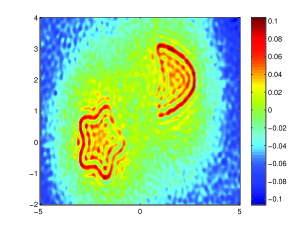
Example 5.1.

We consider the imaging of sound soft obstacles including a circle, a peanut, a kite and a rounded-square. The imaging domain is $\Omega=(-3,3)\times(-3,3)$ with the sampling mesh $201\times 201$. The probe wave wavenumber $k=4\pi$, $N_{s}=N_{r}=128$, and $R_{s}=R_{r}=10$.

Fig. 1: Example 5.1: Imaging results by RTM imaging function (7) with phaseless data. Top row: circle (left) and peanut (right); Bottom row: 5-leaf (left) and diamond (right).

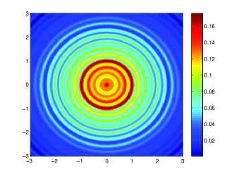
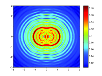
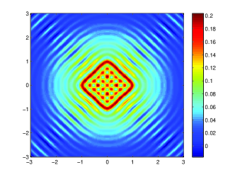
The imaging results are depicted in Figure 1 which show clearly that our imaging algorithm can find the shape and the location of the obstacles using phaseless data regardless of the shapes of the obstacles.

Example 5.2.

We consider the imaging of a 5-leaf obstacle with impedance condition $\eta=5$, a partially coated obstacle with $\eta=5$ in the upper boundary and $\eta=1$ in the lower boundary, a sound hard, and a penetrable obstacle with $n(x)=0.25$. The imaging domain is $\Omega=(-3,3)\times(-3,3)$ with the sampling grid $201\times 201$. The probe wave wavenumber $k=4\pi$, $N_{s}=N_{r}=128$, and $R_{s}=R_{r}=10$.

Fig. 2: Example 5.2: In the top row, a sound hard 5-leaf obstacle (left) and a non-penetrable obstacle with the impedance $\eta=5$ (right). In the bottom row, a partially coated obstacle with $\eta=5$ on the upper boundary and $\eta=1$ on the lower boundary (left) and a penetrable obstacle with $n(x)=1/4$ (right).

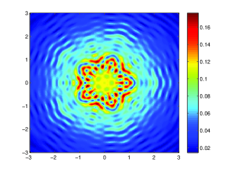
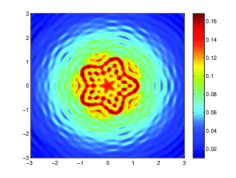
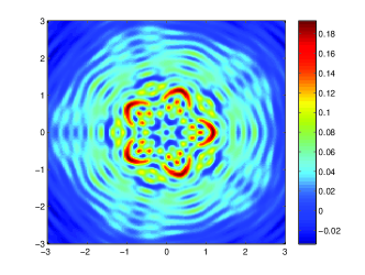
Figure 2 shows the imaging results which demonstrate clearly that our imaging algorithm works for different types of obstacles without using any a prior information of the physical properties of the obstacles.

Example 5.3.

We consider the stability of the imaging function with respect to the additive Gaussian random noises using the phaseless data. We introduce the additive Gaussian noise as follows (see e.g. [3]):

$$|u|_{\rm noise}=|u|+\nu_{\rm noise},$$

where $|u|$ is the synthesized phaseless total field and $\nu_{\rm noise}$ is the Gaussian noise with mean zero and standard deviation $\mu$ times the maximum of the data $|u|$, i.e. $\nu_{\rm noise}=\mu\max|u|{\varepsilon}$, and ${\varepsilon}~{}\thicksim\mathcal{N}(0,1)$.

Fig. 3: Example 5.3: The imaging results using single frequency data added with additive Gaussian noise $\mu=10\%,20\%,30\%,40\%$ from $(a)$ to $(d)$, respectively. The probe wavelength is $\lambda=0.5$ and the sampling number is $N_{s}=N_{r}=256$.

Fig. 4: Example 5.3: The imaging results using multi-frequency data added with additive Gaussian noise $\mu=10\%,20\%,30\%,40\%$ from $(a)$ to $(d)$, respectively. The probe wavelengths are given by $\lambda=1/1.8,1/1.9,1/2.0,1/2.1,1/2.2$ and the sampling number is $N_{s}=N_{r}=256$.

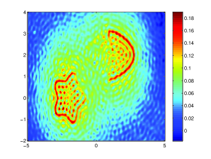
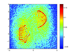
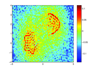
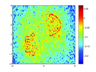
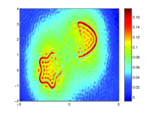
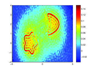
For the fixed probe wavenumber $k=4\pi$, we choose one kite and one 5-leaf in our test. The search domain is $\Omega=(-5,5)\times(-2,4)$ with a sampling $201\times 201$ mesh. We set $R_{s}=10,R_{r}=20$, and $N_{s}=N_{r}=256$. Figure 3 shows the imaging results for the noise level $\mu=10\%,20\%,30\%,40\%$ in the single frequency data, respectively. The imaging results can be improved by superposing the multi-frequency imaging result as shown in Figure 4. The left table in Table 1 shows the noise level, where $\sigma=\mu\max_{x_{r},x_{s}}|u(x_{s},x_{r})|$, $\|u\|_{\ell^{2}}^{2}=\frac{1}{N_{s}N_{r}}\sum^{N_{s},N_{r}}_{s,r=1}|u(x_{s}.x_{r})|^{2}$, $\|\nu_{\rm noise}\|_{\ell^{2}}^{2}=\frac{1}{N_{s}N_{r}}\sum^{N_{s},N_{r}}_{s,r=1}|\nu_{\rm noise}(x_{s},x_{r})|^{2}$.

$\mu$	$\sigma$	$\|u\|_{\ell^{2}}$	$\|\nu_{\rm noise}\|_{\ell^{2}}$
0.1	0.003004	0.013017	0.003007
0.2	0.006009	0.013017	0.005996
0.3	0.009013	0.013017	0.008964
0.4	0.012018	0.013017	0.012008

$\mu$	$\sigma$	$\|u_{s}\|_{\ell^{2}}$	$\|\nu_{\rm noise}\|_{\ell^{2}}$
0.1	0.002859	0.013054	0.002863
0.2	0.005717	0.013054	0.005708
0.3	0.008576	0.013054	0.008572
0.4	0.011435	0.013054	0.011424

Table 1: Example 5.3: The noise level in the case of single frequency data (left) and multi-frequency data (right).

References

- [1] G. Bao, P. Li, and J. Lv. Numerical solution of an inverse diffraction grating problem from phaseless data, J. Opt. Soc. Am. A, 30 (2013): pp. 293-299.
- [2] N. Bleistein, J. Cohen, and J. Stockwell, Mathematics of Multidimensional Seismic Imaging, Migration, and Inversion, Springer, New York, 2001.
- [3] J. Chen, Z. Chen, and G. Huang, Reverse time migration for extended obstacles: acoustic waves, Inverse Problem, 29 (2013), 085005 (17pp).
- [4] J. Chen, Z. Chen, and G. Huang, Reverse time migration for extended obstacles: electromagnetic waves, Inverse Problem, 29 (2013), 085006 (17pp).
- [5] Z. Chen and G. Huang, Reverse time migration for extended obstacles: elastic waves, Science in China Series A: Mathematics, 2015, to appear (in Chinese).
- [6] S.N. Chandler-Wilde, I.G. Graham, S. Langdon, and M. Lindner, Condition number estimates for combined potential boundary integral operators in acoustic scattering, J. Integral Equa. Appli. 21 (2009), pp. 229-279.
- [7] F. Cakoni, D. Colton, and P. Monk, The direct and inverse scattering problems for partially coated obstacles, Inverse Problems 17 (2001), pp. 1997-2015.
- [8] D. Colton, and R. Kress, Inverse Acoustic and Electromagnetic Scattering Theory, 2nd ed., vol. 93 of Applied Mathematical Sciences, Springer-Verlag, Berlin, 1998.
- [9] A.J. Devaney, Structure determination from intensity measurements in scattering experiments, Physical Review Letters, 62 (1989), pp. 2385-2388.
- [10] M. D’Urso, K. Belkebir, L. Crocco, T. Isernia, and A. Litman, Phaseless imaging with experimental data: facts and challenges, J. Opt. Soc. Am. A 25 (2008), pp. 271-281.
- [11] G. Franceschini, M.Donelli, R. Azaro, and A. Massa, Inversion of phaseless total field data using a two-step strategy based on the iterative multiscaling approach, IEEE Trans. Geosci. Remote Sens. 44 (2006), pp. 3527-3539.
- [12] L. Grafakos, Classical and Modern Fourier Analysis, Pearson, London, 2004.
- [13] O. Ivanyshyn, and R.Kress, Identification of sound-soft 3D obstacles from phaseless data, Inverse Problem and Imaing 4 (2010), pp. 131-149.
- [14] O. Ivanyshyn, and R. Kress, Inverse scattering for surface impedance from phase-less far field data, Journal of Computational Physics 230 (2011): pp. 3443-3452.
- [15] M.V. Klibanov, Phaseless inverse scattering problems in threes dimensions, SIAM J. Appl. Math. 74 (2014), pp. 392-410.
- [16] R. Kress, Integral equation methods in inverse acoustic and electromagnetic scattering, In: Boundary Integral Formulations for Inverse Analysis (Ingham and Wrobel, eds), Computational Mechanics Publications, Southampton, 1997, pp. 67- 92.
- [17] R. Kress, and W. Rundell, Inverse obstacle scattering with modulus of the far field pattern as data,. H. W. Engl et al. (eds.), Inverse Problems in Medical Imaging and Nondestructive Testing, Springer Vienna, 1997.
- [18] R. Leis, Initial Boundary Value Problems in Mathematical Physics, B.G. Teubner, Stuttgart, 1986.
- [19] A. Litman, and K. Belkebir, Two-dimensional inverse profiling problem using phaseless data, J. Opt. Soc. Am. A, 23 (2006), pp. 2737-2746.
- [20] W. McLean, Strongly Elliptic Systems and Boundary Integral Equations, Cambridge University Press, Cambridge, 2000
- [21] P. Monk, Finite Element Methods for Maxwell’s Equations, Clarendon Press, Oxford, 2003.
- [22] F. Oberhettinger and L. Badii. Tables of Laplace Transforms, Springer-Verlag, Heidelberg, 1973.
- [23] R. Potthast, Point-sources and Multipoles in Inverse Scattering Theory, Chapman and Hall/CRC, Boca Raton, Florida, 2001.
- [24] G. N. Watson. A Treatise on the Theory of Bessel Functions. Cambridge University Press, Cambridge, 1995.
- [25] B. Zhang On transmission problems for wave propagation in two locally perturbed half-spaces, Math. Proc. Camb. Phil. Soc. 115 (1994), pp. 545-558.
- [26] W. Zhang, L. Li, and F. Li. Inverse scattering from phaseless data in the free space, Science in China Series F: Information Sciences 52 (2009), pp. 1389-1398.