Central limit theorems for some set partition statistics

Abstract.

We prove the conjectured limiting normality for the number of crossings of a uniformly chosen set partition of $[n]=\{1,2,\ldots,n\}$. The arguments use a novel stochastic representation and are also used to prove central limit theorems for the dimension index and the number of levels.

1. Introduction

Let $\lambda$ be a partition of the set $[n]=\{1,2,\ldots,n\}$, so $1|2|3,12|3,13|2,1|23,123$ are the five partitions of $[3]$. The enumerative theory of “supercharacters” leads to the statistics

(1.1) $$d(\lambda)=\sum_{i}(M_{i}-m_{i}+1)\ \ \text{ and }\ \ cr(\lambda)=\#\text{ of crossings of }\lambda.$$

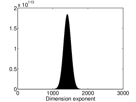
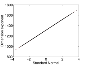
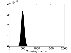
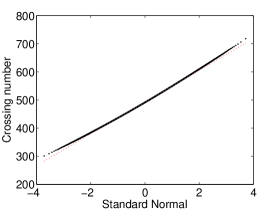
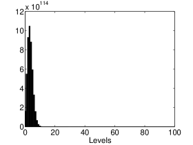
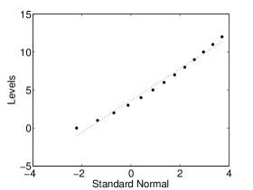
In $d(\lambda)$, the sum is over the blocks of $\lambda$ and $M_{i}$ ($m_{i}$) is the largest (smallest) element of the block $i$. The statistic $cr(\lambda)$ counts $i<i^{\prime}<j<j^{\prime}$ with $i,j$ adjacent elements of the same block and $i^{\prime},j^{\prime}$ adjacent elements of the same block (). In a companion paper [3] the moments of $d(\lambda)$ and $cr(\lambda)$ are determined as explicit linear combinations of Bell numbers $B_{n}$. Numerical computations (see Figures 1 and 2) suggests that normalized by their mean and variance, these statistics have approximate normal distributions. Figures 1 – 3 are based on exact counts from our new algorithms [3]. Figures 1 and 2 suggest good agreement with the normal approximation for dimension index and crossings. Figure 3 shows slower convergence for levels and suggests a search for finite sample correction terms. We found the limiting normality challenging to prove using available techniques (eg. moments, Fristedt’s method of conditioned limit theorems [9], or Stein’s method [4]). Indeed, the limiting normality of $cr(\lambda)$ is conjectured in [13].

Figure 1. Histogram of the dimension exponent counts for $n=100$ and the associated Q-Q plot.

Figure 2. Histogram of the crossing number counts for $n=100$ and the associated Q-Q plot.

Figure 3. Histogram of the level counts for $n=100$ and the associated Q-Q plot.

A key ingredient of the present paper is a stochastic algorithm for generating a random set partition due to Stam [24]. Supplementing this with some novel probabilistic ideas allows standard “delta method” techniques to finish the job.

Brief reviews of the extensive enumerative, algebraic and probabilistic aspects of set partitions are in [16] and [25]. The book of Mansour [18] contains applications to computer science and much else. An important paper combining many of the statistics we work with is [2]. The companion paper [3] has an extensive review. It also summarizes the literature on supercharacters. Briefly, these are natural characters $\chi_{\lambda}$ on the uni-upper triangular matrix group $U_{n}({\mathbb{F}}_{q})$ which are indexed by set partitions. The representation corresponding to $\chi_{\lambda}$ has dimension $q^{d(\lambda)}$. The (usual) inner product between $\chi_{\lambda}$ and $\chi_{\mu}$ is $<\chi_{\lambda},\chi_{\mu}>=q^{cr(\lambda)}\delta_{\lambda,\mu}$. This suggests understanding how $d(\lambda)$ and $cr(\lambda)$ vary for typical set partitions.

There are many codings of a set partition. One needed below codes $\lambda$ as a sequence $x_{1},x_{2},\cdots,x_{n}$ with $x_{i}=j$ if and only if $i$ is in block $j$ of $\lambda$. Thus $135|24|6|7$ corresponds to $1,2,1,2,1,3,4$. If $a_{i}=x_{i}-1$, $a_{1},a_{2},\cdots,a_{n}$ is a restricted growth sequence: $a_{1}=0$ and $a_{i+1}\leq 1+\max(a_{1},\cdots,a_{i})$ for $1\leq i\leq n-1$. This standard coding is discussed in [16, page 416]. For this coding, let

(1.2) $$L(\lambda)=\left|\{i:x_{i+1}=x_{i}\}\right|$$

the number of levels of $\lambda$. This is used as an example of the present techniques. See [18, Chapter 4] for further references.

The main theorems proved use $\alpha_{n}$, the positive real solution of $ue^{u}=n+1$ (so $\alpha_{n}=\log(n)-\log\log(n)+o(1)$ [8]). Let $\Pi(n)$ be the set of partitions of $[n]$. Throughout, $\lambda$ is uniformly chosen in $\Pi(n)$.

Theorem 1.1.

The number of levels $L(\lambda)$ has $\mu_{n}^{L}={\mathbb{E}}(L(\lambda))=(n-1)\frac{B_{n-1}}{B_{n}}\sim\log(n)$ and $\left(\sigma_{n}^{L}\right)^{2}={\rm VAR}(L(\lambda))=(n-1)\frac{B_{n-1}}{B_{n}}+n(n-1)\frac{B_{n-2}}{B_{n}}-(n-1)^{2}\frac{B_{n-1}^{2}}{B_{n}^{2}}\sim\log(n).$ Normalized by its mean and standard deviation, $L(\lambda)$ has an approximate standard normal distribution

$${\bf P}\left(\frac{L(\lambda)-\mu_{n}^{L}}{\sigma_{n}^{L}}\leq x\right)\to\frac{1}{\sqrt{2\pi}}\int_{-\infty}^{x}e^{-\tau^{2}/2}d\tau$$

for all fixed $x$ as $n\to\infty$.

Theorem 1.2.

The dimension index $d(\lambda)$ has $\mu_{n}^{d}={\mathbb{E}}(d(\lambda))=\frac{\alpha_{n}-2}{\alpha_{n}}n^{2}+O\left(\frac{n}{\alpha_{n}}\right)$ and $\left(\sigma_{n}^{d}\right)^{2}={\rm VAR}(d(\lambda))=\left(\frac{\alpha_{n}^{2}-7\alpha_{n}+17}{\alpha_{n}^{3}(\alpha_{n}+1)}\right)n^{3}+O\left(\frac{n^{2}}{\alpha_{n}}\right).$ Normalized by its mean and standard deviation, $d(\lambda)$ has an approximate standard normal distribution

$${\bf P}\left(\frac{d(\lambda)-\mu_{n}^{d}}{\sigma_{n}^{d}}\leq x\right)\to\frac{1}{\sqrt{2\pi}}\int_{-\infty}^{x}e^{-\tau^{2}/2}d\tau$$

for all fixed $x$ as $n\to\infty$.

Theorem 1.3.

The number of crossings $cr(\lambda)$ has $\mu_{n}^{cr}={\mathbb{E}}(cr(\lambda))=\frac{2\alpha_{n}-5}{4\alpha_{n}^{2}}n^{2}+O\left(\frac{n}{\alpha_{n}}\right)$ and $\left(\sigma_{n}^{cr}\right)^{2}={\rm VAR}(cr(\lambda))=\frac{3\alpha_{n}^{2}-22\alpha_{n}+56}{9\alpha_{n}^{3}(\alpha_{n}+1)}n^{3}+O\left(\frac{n^{2}}{\alpha_{n}}\right).$ Normalized by its mean and standard deviation, $cr(\lambda)$ has an approximate standard normal distribution

$${\bf P}\left(\frac{cr(\lambda)-\mu_{n}^{cr}}{\sigma_{n}^{cr}}\leq x\right)\to\frac{1}{\sqrt{2\pi}}\int_{-\infty}^{x}e^{-\tau^{2}/2}d\tau$$

for all fixed $x$ as $n\to\infty$.

Section 2 of this paper explains Stam’s algorithm and shows how it gives a useful heuristic picture of what a random set partition “looks like”. The limit theorem for levels is proved in Section 3 as a simple illustration of our proof technique. The dimension index and number of crossings require further ideas. They are given separate proofs in Sections 4 and 5.

Notation

Throughout, we use the stochastic order symbols $O_{p}$ and $o_{p}$. If $X_{n}$ for $1\leq n<\infty$ is a sequence of real valued random variables and $a_{n}$ is a sequence of real numbers, write $X_{n}=O_{p}(a_{n})$ if for every $\epsilon>0$ and some $\eta>0$, which may depend on $\epsilon$, there is $N$ so that ${\bf P}\{\left|X_{n}\right|\leq\eta\left|a_{n}\right|\}>1-\epsilon$ for all $n>N$. Write $X_{n}=o_{p}(a_{n})$ if for every $\epsilon>0$ and $\eta>0$ there is $N$ so that ${\bf P}\{\left|X_{n}\right|<\eta\left|a_{n}\right|\}>1-\epsilon$ for all $n>N$. For background, examples and many variations see Pratt [21], Lehman [17], or Serfling [22]. We say two sequences of random variables are weak star close if their distributions are close in Lévy metric.

2. Stam’s algorithm and set partition heuristics

Write $\Pi(n)$ for the set partitions of $[n]=\{1,2,\cdots,n\}$ and $B_{n}=\left|\Pi(n)\right|$ for the $n$th Bell number (sequence A000110 of Sloane’s [23]). To help evaluate asymptotics it is helpful to have

$$\frac{B_{n+1}}{B_{n}}=\frac{n}{\alpha_{n}}+\frac{1}{2}\frac{\alpha_{n}}{(1+\alpha_{n})^{2}}+O\left(\frac{\alpha_{n}}{n}\right)$$

$$\frac{B_{n+k}}{B_{n}}=\frac{(n+k)!}{n!\alpha_{n}^{k}}\left(1+O\left(\frac{k}{n\alpha_{n}}\right)\right)$$

$$\frac{\alpha_{n+k}}{\alpha_{n}}=1+O\left(\frac{k}{n\log(n)}\right)$$

which are valid for fixed $k$ as $n\to\infty$. See, for instance, [8]. Dobinski’s identity [7, 20]

(2.1) $$B_{n}=\frac{1}{e}\sum_{m=1}^{\infty}\frac{m^{n}}{m!}$$

shows that for fixed $n\in\{0,1,2,\cdots\}$

(2.2) $$\mu_{n}(m)=\frac{1}{eB_{n}}\frac{m^{n}}{m!}$$

is a probability measure on $\{1,2,3,\cdots\}$. Stam [24] uses this measure to give an elegant algorithm for choosing a uniform random element of $\Pi(n)$.

Stam’s Algorithm

1. Choose $M$ from $\mu_{n}$.

2. Drop $n$ labelled balls uniformly into $M$ boxes.

3. Form a set partition $\lambda$ of $[n]$ with $i$ and $j$ in the same block if and only if balls $i$ and $j$ are in the same box.

Of course, after choosing $M$ and dropping balls, some of the boxes may be empty. Stam [24] shows that the number of empty boxes has (exactly) a Poisson distribution and is independent of the generated set partition. This implies that the number of boxes $M$ drawn from $\mu_{n}$ at (2.2) has the same limiting distribution as the number of blocks in a random $\lambda\in\Pi(n)$. This is a well studied random variable. It will emerge that the fluctuations of $M$ are the main source of randomness in Theorems 1.1 – 1.3. Results of Hwang [11] prove the following normal limit theorem (Hwang also has an error estimate).

Theorem 2.1.

For $M$ chosen from $\mu_{n}$ of (2.2), as $n\to\infty$

$$\mu_{n}^{M}:={\mathbb{E}}(M)=\frac{B_{n+1}}{B_{n}}=\frac{n}{\alpha_{n}}+O\left(\frac{1}{\alpha_{n}}\right)$$

and

$$\left(\sigma_{n}^{M}\right)^{2}:={\rm VAR}(M)=\frac{B_{n+2}}{B_{n}}-\frac{B_{n+1}^{2}}{B_{n}^{2}}=\frac{n}{\alpha_{n}^{2}}+O\left(\frac{n}{\alpha_{n}^{3}}\right).$$

Normalized by its mean and standard deviation, $M$ has an approximate standard normal distribution.

Heuristic I. Stam’s algorithm gives a useful intuitive way to think about a random element of $\Pi(n)$. It behaves practically the same as a uniform multinomial allocation of $n$ labelled balls into $m=n/\log(n)$ boxes. The arguments in the following sections make this precise. It appears to us that many of the features previously treated in the beautiful paper of Fristedt [9] can be treated by the present approach. Note that Fristedt treated features that only depend on block sizes (largest, smallest, number of boxes of size $i$). None of our statistics have this form.

Heuristic II. Fristedt’s arguments randomize $n$. This makes the block variables, $N_{i}(\lambda)=\#\text{ blocks of size }i$, independent allowing standard probability theorems to be used. At the end, a Tauberian argument (dePoissonization) is used to show that the theorems hold for fixed $n$. The present argument fixes $n$ and randomizes the number of blocks. This results in a “balls in boxes” problem with many tools available. At the end, an Abelian argument shows that the appropriate limit theorem holds when $m$ fluctuates. See [10] for background on this use of Abelian and Tauberian theorems. There are many variants of Poissonization in active use. We do not see how to abstract Stam’s algorithm to other combinatorial structures.

We conclude this section with a simple illustration of Stam’s algorithm. From (2.2), $\mu_{n}(m)=\frac{1}{eB_{n}}\frac{m^{n}}{m!}$ is a probability measure on $\{1,2,3,\cdots\}$. Thus for $-n<d<\infty$

(2.3) $${\mathbb{E}}_{n}(M^{d})=\frac{1}{eB_{n}}\sum_{m=1}^{\infty}\frac{m^{n+d}}{m!}=\frac{B_{n+d}}{B_{n}}.$$

Let us apply this to compute the moments for $L(\lambda)$, the number of levels of $\lambda\in\Pi(n)$. From the definition (1.2), given $M$, $L(\lambda)=X_{1}+\cdots+X_{n-1}$ where $X_{i}$ is the indicator random variable of the event that balls $i$ and $i+1$ are dropped into the same box. By inspection, the $X_{i}$ are independent with ${\bf P}(X_{i}=1)=\frac{1}{M}$. Thus

(2.4) $${\mathbb{E}}_{n}(L(\lambda))={\mathbb{E}}_{n}{\mathbb{E}}\left(L(\lambda|M)\right)={\mathbb{E}}_{n}\left(\frac{n-1}{M}\right)=(n-1)\frac{B_{n-1}}{B_{n}}.$$

The standard identity

$${\rm VAR}(Z)={\mathbb{E}}({\rm VAR}(Z|W))+{\rm VAR}({\mathbb{E}}(Z|W))$$

for any random variables $Z$ and $W$ such that the moments exist, shows that

(2.5) $${\rm VAR}_{n}(L(\lambda))=(n-1)\frac{B_{n-1}}{B_{n}}+n(n-1)\frac{B_{n-2}}{B_{n}}-(n-1)^{2}\frac{B_{n-1}^{2}}{B_{n}^{2}}.$$

More generally, this provides an alternative approach to [3] for showing that the moments of statistics $T(\lambda)$ are shifted Bell polynomials. It requires ${\mathbb{E}}_{n}(T(\lambda)|m)$ to be a Laurent polynomial in $m$. As an example, Stam worked with $W_{i}(\lambda)$, the size of the block in $\lambda$ containing $i$, $1\leq i\leq n$. Then, any polynomial in the $\{W_{i}\}_{i=1}^{n}$ has expectation a shifted Bell polynomial; for example, $W_{i}^{k}$ and $W_{i}W_{j}$. Stam proves that $W_{i}$ is approximately normal.

3. Proof of Theorem 1.1

Theorem 1.1 is proved here as a simple illustration of our technique. Conditioning on $M$ in Stam’s algorithm, classical “balls in bins” central limit theorems are used to prove the limiting normality uniformly in $M$ and standard $\delta$-method arguments are used to complete the proof.

Proof of Theorem 1.1.

The moments of the level statistic $L(\lambda)$ are computed in (2.4) and (2.5). Conditional on $M$, $L(\lambda)=X_{1}+\cdots+X_{n-1}$ with $X_{i}$ independent identically distributed binary variables with ${\bf P}(X_{i}=1)=1/M$. Thus conditioned on $M$,

$${\mathbb{E}}(L(\lambda)\mid M)=\frac{n-1}{M},\ \ \ \text{ and }\ \ \ {\rm VAR}(L(\lambda)\mid M)=\frac{n-1}{M}\left(1-\frac{1}{M}\right).$$

and, normalized by its conditional mean and variance, $L(\lambda)$ has a standard normal limiting distribution provided $n/M\to\infty$. In the present case, $M=M_{n}$ is a random variable. From Theorem 2.1, as $n$ tends to infinity

(3.1) $$\frac{M_{n}-\mu_{n}^{M}}{\sigma_{n}^{M}}\to N(0,1)\text{ with }\mu_{n}^{M}\sim\frac{n}{\alpha_{n}},(\sigma_{n}^{M})^{2}\sim\frac{n}{\alpha_{n}^{2}}.$$

This implies

(3.2) $$\frac{n}{M_{n}}=\alpha_{n}+O_{p}\left(\frac{1}{\sqrt{n}}\right).$$

To be precise, write $M_{n}=\mu_{n}^{M}+Z_{n}\sigma_{n}^{M}$ with $Z_{n}=\frac{M_{n}-\mu_{n}^{M}}{\sigma_{n}^{M}}$. Then

(3.3) $$\frac{n}{M_{n}}=\frac{n}{\mu_{n}^{M}+Z_{n}\sigma_{n}^{M}}=\frac{n}{\mu_{n}^{M}\left(1+\frac{Z_{n}}{\sigma_{n}^{M}}\mu_{n}^{M}\right)}=\frac{n}{\mu_{n}}\left(1+\frac{Z_{n}}{\mu_{n}^{M}}\sigma_{n}^{M}+O\left(\left(\frac{Z_{n}\sigma_{n}^{M}}{\mu_{n}^{M}}\right)^{2}\right)\right).$$

From Theorem 2.1, $n/\mu_{n}^{M}=\alpha_{n}+O(\alpha_{n}/n)$, $\sigma_{n}^{M}/\mu_{n}^{M}=O(1/\sqrt{n})$. Since $Z_{n}=O_{p}(1)$, (3.2) follows.

Thus, with probability close to 1 with respect to $M$ we have that $L(\lambda)$ conditioned on $M$ is weak star close to a Gaussian with mean

$$\mu^{M}=\frac{n-1}{M}=\alpha_{n}+O_{p}(n^{-1/2})$$

and standard deviation

$$\sigma^{M}=\sqrt{\frac{n-1}{M}\left(1-\frac{1}{M}\right)}=\sqrt{\alpha_{n}}+O_{p}(n^{-1/2}).$$

Thus, with high probability over $M$, the conditional distribution on $L(\lambda)$ is weak star close to $N(\alpha_{n},\sqrt{\alpha_{n}})$. Therefore, the overall distribution of $L(\lambda)$ is also close to this normal distribution.

∎

4. Proof of Theorem 1.2

In outline, the proof proceeds by choosing a random $\lambda\in\Pi(n)$ using Stam’s algorithm. Conditioning on the chosen $m$ reduces the problem to a slightly non-standard balls in boxes problem. Given $m$, it is shown that $d(\lambda)=nm-2m^{2}+O_{p}(m^{3/2})$ so that the fluctuations in $d(\lambda)$ are driven by the fluctuations in $m$. These are asymptotically normally distributed with mean and variance $\left(\frac{n}{\alpha_{n}},\frac{n}{\alpha_{n}^{2}}\right)$. From Theorem 2.1 above, a simple averaging argument completes the proof. The first proposition treats the balls in boxes argument. It proves more than is needed. The argument is useful for statistics such as $T(\lambda)=\sum_{i}M_{i}$ where the sum runs over the blocks of $\lambda$ indexed by $i$ and $M_{i}$ is the maximum element in the $i$th block.

The first step in the proof is to prove the appropriate approximation conditional on $m$. While it would be of interest to explore this for general $n$, $m$, we content ourselves with proving what is needed for Theorem 1.2. From Theorem 2.1 the relevant values of $m$ are $\frac{n}{\alpha_{n}}+\frac{c\sqrt{n}}{\log(n)}$ for large fixed values of $c$. This explains the choice in the next lemma.

Lemma 4.1.

Fix a large number $C$. Let $n$ balls labeled $1,2,\cdots,n$ be dropped uniformly at random into $m$ boxes with $m=\frac{n}{\alpha_{n}}+\frac{c\sqrt{n}}{\log(n)}$. For $\left|c\right|\leq C$. Let

$$D_{n}=\sum_{i=1}^{m}\left(M_{i}-m_{i}+1\right)$$

with $M_{i}$ the maximum label in box $i$ and $m_{i}$ the minimum label of box $i$. $M_{i}-m_{i}$ is omitted if box $i$ is empty. Then $D_{n}=nm-2m^{2}+O_{p,C}(m^{3/2})$ uniformly in $\left|c\right|\leq C$.

Proof.

Consider an infinite supply of balls labelled $1,2,3,\ldots$ dropped uniformly at random into $m$ boxes. Let $W_{i}$ $1\leq i\leq m$ be the waiting time until $i$ boxes have been filled. Thus $W_{i}=1$, $W_{2}-W_{1}$ is GEOMETRIC($1/m$), $W_{3}-W_{2}$ is GEOMETRIC($2/m$), …, $W_{n}-W_{n-1}$ is GEOMETRIC($(m-1)/m$) and all these differences are independent. Here, if $X$ is GEOMETRIC($\theta$), ${\bf P}(X=j)=\theta^{j-1}(1-\theta)$, ${\mathbb{E}}(X)=1/\theta$, and ${\rm VAR}(X)=\frac{1}{\theta}\left(\frac{1}{\theta}-1\right)$. Let $E_{t}$ be the number of empty boxes at time $t$ and $L_{t}$ be the largest $\ell$ so that $W_{\ell}\leq t$. If $L_{m}\leq t$ all boxes are non-empty at time $t$ and $E_{t}=0$. More generally, $L_{t}=m-E_{t}$.

The sum $\sum_{i=1}^{m}m_{i}$ is $W_{1}+\cdots+W_{L_{n}}$. This sum may be controlled by showing that $E_{n}$ is bounded with high probability and then bounding the sum by Chebychev bounds. The same argument works for $\sum_{i=1}^{m}M_{i}$. Toward this end, represent

$$E_{n}=\sum_{i=1}^{m}X_{i}\ \ \ \text{ where }\ \ \ X_{i}=\begin{cases}1&\text{ box $i$ is empty after $n$ balls}\\ 0&\text{ box $i$ is not empty after $n$ balls}\end{cases}.$$

$${\mathbb{E}}\left(E_{n}\right)=m\left(1-\frac{1}{m}\right)^{n},\ \ \ {\rm VAR}(E_{n})=m\left(1-\frac{1}{m}\right)^{n}+m(m-1)\left(1-\frac{1}{m}\right)^{n}-m^{2}\left(1-\frac{1}{m}\right)^{2n}.$$

By elementary estimates

(4.1) $${\mathbb{E}}\left(E_{n}\right)=1+O\left(\frac{C}{\sqrt{n}}\right),\ \ \ {\rm VAR}(E_{n})=1+O\left(\frac{C}{\sqrt{n}}\right).$$

Indeed, $m\left(1-\frac{1}{m}\right)^{n}=e^{\log(m)-\frac{n}{m}+O\left(\frac{n}{m^{2}}\right)}$. Using the assumption $m=\frac{n}{\alpha_{n}}+\frac{c\sqrt{n}}{\log(n)}$, $\log(m)=\alpha_{n}+O\left(\frac{c}{\sqrt{n}}\right),\frac{n}{m}=\alpha_{n}+O\left(\frac{1}{\sqrt{n}\log(n)}\right).$ This gives the first result in (4.1), the second follows similarly. By classical results [1], $E_{n}$ is approximately POISSON(1) distributed with an explicit total variation error but this is not needed.

Consider next

$$S_{n}=W_{1}+\cdots+W_{m}=mW_{1}+(m-1)(W_{2}-W_{1})+\cdots+2(W_{m-1}-W_{m-2})+(W_{m-1}-W_{m}).$$

(4.2) $${\mathbb{E}}(S_{n})=\frac{m}{1}+\frac{m-1}{\frac{m-1}{m}}+\cdots+\frac{1}{\frac{1}{m}}=m^{2}$$

(4.3) $${\rm VAR}(S_{n})=\sum_{i=1}^{m-1}(m-i)^{2}\frac{m}{m-i}\left(\frac{m}{m-i}-1\right)=\sum_{i=1}^{m}mi=m\frac{m(m-1)}{2}\sim\frac{m^{3}}{2}.$$

Consider next the sum of the box maxima. Drop balls labelled $n,n-1,\cdots,1$ sequentially into $m$ boxes. If the new arrivals are at times $\widetilde{W_{1}},\widetilde{W_{2}},\cdots,\widetilde{W_{m}}$, the box maxima are $n-(\widetilde{W_{1}}-1),n-(\widetilde{W_{2}}-1),\ldots,n-(\widetilde{W_{m}}-1)$. The sum

$$\widetilde{S_{n}}=\sum_{i=1}^{m}m_{i}=nm-\left(\widetilde{W_{1}}+\cdots+\widetilde{W_{m}}\right)+n.$$

Thus

(4.4) $${\mathbb{E}}(\widetilde{S_{n}})=n(m+1)-m^{2}$$

(4.5) $${\rm VAR}(\widetilde{S_{n}})=m\frac{m(m-1)}{2}.$$

The random variable of interest is

$$D_{n}=\sum_{i=1}^{m}(M_{i}-m_{i}+1)=\widetilde{S_{n}}-S_{n}-\sum_{i=L_{n}+1}^{m}\left(\widetilde{W_{i}}-W_{i}\right)+m.$$

The sum $\sum_{i=L_{n}+1}^{m}\widetilde{W_{i}}\leq E_{n}\widetilde{W_{m}}.$ From the coupon collectors problem $\widetilde{W_{m}}$ is of stochastic order $m\log(m)\sim n$ and $E_{n}$ is stochastically bounded. A similar argument holds with $\widetilde{W_{i}}$ replaced by $W_{i}$. It follows that the sum $\sum_{i=L_{n}+1}^{m}\left(\widetilde{W_{i}}-W_{i}\right)=O_{p}(n).$ Combining terms

$$D_{n}=\widetilde{S_{n}}-\widetilde{S_{n}}+m+O_{p}(n)=nm+\left(\widetilde{S_{n}}-{\mathbb{E}}(\widetilde{S_{n}})\right)-\left(S_{n}-{\mathbb{E}}(S_{n})\right)+O_{p}(n).$$

By Chebychev’s inequality $\left|S_{n}-{\mathbb{E}}(S_{n})\right|$ and $\left|\widetilde{S_{n}}-{\mathbb{E}}(\widetilde{S_{n}})\right|$ are both $O_{p}(m^{3/2})$. It follows that $D_{n}=nm-2m^{2}+O_{p}(m^{3/2})$. ∎

Proof of Theorem 1.2.

To finish the proof of Theorem 1.2 note that conditional on $M$

$$d(\lambda)=nM-2M^{2}+O_{p}(M^{3/2}).$$

This is weak star close to

$$N\left(\frac{n^{2}}{\alpha_{n}}-\frac{2n^{2}}{\alpha_{n}^{2}},\frac{n^{3/2}}{\alpha_{n}}\right)+O_{p}\left(\frac{n}{\alpha_{n}}\right)^{3/2}.$$

Since $(n/\alpha_{n})^{3/2}$ is much smaller than the standard deviation of the normal, this is in turn close to

$$N\left(\frac{n^{2}}{\alpha_{n}}-\frac{2n^{2}}{\alpha^{2}},\frac{n^{3/2}}{\alpha_{n}}\right).$$

This completes the proof. ∎

5. Proof of Theorem 1.3

This section contains the proof of Theorem 1.3. Our approach is to compare the crossing statistic to the dimension statistic, which by Theorem 1.2 is known to be normally distributed.

Proof.

To analyze the distribution of the crossing number, we compare it to the dimension index. We do this by producing a uniform random set partition $\lambda$ in the following unusual way:

• Pick $M$ from $\mu_{n}$.

• Pick a uniform random set partition $\mu$ for that $m$ according to Stam’s algorithm.

• Let $\lambda$ be a uniform random set partition conditional on the event that the set of minimum elements of blocks of $\lambda$ is the set of minimum elements of blocks on $\mu$ and that the set of maximum elements of blocks of $\lambda$ equals the set of maximum elements of blocks of $\mu$.

This third step can be accomplished in the following way, assigning the elements of $[n]$ to blocks in order. We begin with no blocks and add elements to blocks one at a time, sometimes creating new blocks. If an element $k$, where $k$ is the maximum element of some block of $\mu$ is added to a block in $\lambda$, we declare that block closed. After having assigned the first $k$ elements to blocks in $\lambda$, we assign $k+1$ to a uniform random un-closed block, unless $k+1$ is the minimum element of some block of $\mu$, in which case we assign $k+1$ to a new block of $\lambda$. This procedure clearly produces a uniform $\lambda$ subject to the restriction on the minimum and maximum elements of blocks.

On the other hand, this method of choosing $\lambda$ gives us a reasonable way to analyze $cr(\lambda)$. In particular, the crossing number of $\lambda$ equals the number of pairs of a $j\in[n]$ and a block $B$ in $\lambda$ with

• $j\not\in B$

• $j$ not the first element of its block

• $\max(B)>j$

• The element of $B$ immediately preceding $j$ is larger than the element of $j$’s block immediately preceding $j$

We note that this is easy to analyze given the procedure above for choosing $\lambda$. Suppose that when $k$ is being added to $\lambda$ that there are $a_{k}$ blocks of $\lambda$ currently open. If $k$ is the first element of its block, then we have no crossings with $j=k$. Otherwise, we claim that the number of crossings with $j=k$ (which we call $X_{k}$) has distribution given by the discrete uniform random variable on $[0,a_{k}-1]$. In particular, if the open blocks are $B_{1},\ldots,B_{a_{k}}$ whose element immediately preceding $k$ is $m_{1}<m_{2}<\ldots<m_{a_{k}}$, then $X_{k}=k-i$ if $k$ is assigned to block $B_{i}$. Note furthermore, that the $a_{k}$ are determined by $\mu$ and that the $X_{k}$ are independent conditional on $\mu$. Since $cr(\lambda)=\sum_{k}X_{k}$ is a sum of independent random variables, it is easy to see that conditioned on $\mu$ that with high probability $cr(\lambda)$ is weak star close to

$$N\left(\sum_{k\textrm{ not a minimum}}\frac{a_{k}-1}{2},\sqrt{\sum_{k\textrm{ not a minimum}}\frac{a_{k}^{2}-1}{12}}\right).$$

We note that a given block contributes to $a_{k}$ if and only if $k$ is between is minimum and maximum values. Therefore,

$$\sum_{k=1}^{n}(a_{k}-1)=\left(\sum_{i=1}^{m}M_{i}-m_{i}\right)-n=nm-2m^{2}+O_{p}(m^{3/2}).$$

On the other hand, the sum over $a_{k}$ at the start of blocks is the number pairs of blocks that overlap. Note that for $m=n/\alpha_{n}+o_{p}(n/\log^{2}(n))$, that any given block has $n/2$ between its minimum and maximum with probability $1-O(m^{-1/2})$. Thus, for $m$ in this range, the expected number of pairs of non-overlapping blocks is $O(m^{3/2})$. Thus,

$$\sum_{k\textrm{ not a minimum}}\frac{a_{k}-1}{2}=nm/2-5m^{2}/4+O_{p}(m^{3/2}).$$

It is also easy to see that

$$\sum_{k\textrm{ not a minimum}}(a_{k}^{2}-1)=n^{2}m(1+o_{p}(1))=\frac{n^{3}}{\alpha_{n}}(1+o_{p}(1)).$$

Therefore, with probability approaching $1$ over the choice of $m$, the distribution of $\lambda$ conditioned on $m$ is close to

$$N\left(nm/2-5m^{2}/4,\frac{n^{3/2}}{\sqrt{12\alpha_{n}}}\right).$$

This can be rewritten (up to small error) as the sum of $(n/2+5n/(2\alpha_{n}))(m-n/\alpha_{n})$ and a variable with distribution

$$N\left(\frac{n^{2}}{2\alpha_{n}}-\frac{5n^{2}}{4\alpha_{n}^{2}},\frac{n^{3/2}}{\sqrt{12}\alpha_{n}}\right).$$

On the other hand, by Theorem 2.1, $(n/2+5n/(2\alpha_{n}))(m-n/\alpha_{n})$ is approximated by an independent normal weak star close to

$$N\left(0,\frac{n^{3/2}}{2\alpha_{n}}\right).$$

Thus, the distribution of $cr(\lambda)$ is close in cdf distance to this sum of independent normals, which is given by

$$N\left(\frac{n^{2}}{2\alpha_{n}}-\frac{5n^{2}}{4\alpha_{n}^{2}},\frac{n^{3/2}}{\sqrt{3}\alpha_{n}}\right).$$

This completes the proof. ∎

References

• [1] S. Chatterjee, P. Diaconis, and E. Meckes, Exhchangable pairs and Poisson approximation. Prob. Surveys (2005).
• [2] W. Y. C. Chen, E. Y. P. Deng, R. R. X. Du, R. P. Stanley and C. H. Yan, Crossings and nestings of matchings and partitions. Trans. Amer. Math. Soc. 359 (4) (2007), 1555–1575.
• [3] B. Chern, P. Diaconis, D. M. Kane, and R. C. Rhoades, Closed expressions for set partition statistics. Research in the Mathematical Sciences 1 2, (2014).
• [4] L. Chen, L. Goldstein, and Q-M. Shao, Normal approximation by Stein’s method, Springer Verlag (2010).
• [5] L. Chen, Q-M. Shao, Normal Approximation under local dependence, Ann. Probab. Volume 32, Number 3 (2004), 1727-2303
• [6] P. Diaconis and I. M. Isaacs, Supercharacters and superclasses for algebra groups. Trans. Amer. Math. Soc. 360 (2008), 2359–2392.
• [7] G. Dobinski, Summirung der reine nm/m!superscript𝑛𝑚𝑚\sum n^{m}/m! for m=1,2,3,4,5,𝑚12345m=1,2,3,4,5,\ldots. Grunet. Archiv. 61 (1877), 333–336.
• [8] N. G. de Bruijn, Asymptotic Methods in Analsysis. Dover, N.Y.
• [9] B. Fristedt, The structure of random partitions of large sets. Technical Report Dept. of Mathematics, University of Minnesota (1987), 86–154.
• [10] G. H. Hardy, Divergent series. Oxford Univ. Press (1991).
• [11] H.K. Hwang, On Convergence Rates in the Central Limit Theorems for Combinatorial Structures. European J. Combin. 19 (1998), no. 3, 329–343.
• [12] A. Kasraoui, Average values of some Z𝑍Z parameters in random set partitions. Electronic J. Combinatorics, Volume 18, Issue 1 (2011) #P228.
• [13] A. Kasraoui, On the limiting distribution of some numbers of crossings in set partitions. arxiv:1301,6546 (2013).
• [14] A. Kasraoui and J. Zeng, Distribution of crossings, nestings and alignments of two edges in matchings and partitions. Electron. J. Combin. 13 (2006), no. 1, Research Paper 33, 12 pp.
• [15] A. Knopfmacher, T. Mansour, and S. Wagner, Records in set partitions. Electronic Journal of Combinatorics 17 (2010) R109 (14pp.).
• [16] D. Knuth, The art of computer programming. Vol 4A. Addison-Wesley.
• [17] E. Lehman, Elemnts of large sample theory. Springer (1999).
• [18] T. Mansour, Combinatorics of set partitions. Discrete Mathematics and its Applications (Boca Raton). CRC Press, Boca Raton, FL, 2013.
• [19] A. Nijenhuis and H. S. Wilf, Combinatorial algorithms. For computers and calculators. Second edition. Computer Science and Applied Mathematics. Academic Press, Inc. [Harcourt Brace Jovanovich, Publishers], New York-London, 1978.
• [20] J. Pitman, Some probabilistic aspects of set partitions. Amer. Math. Monthly, 104 (1997), 201–209.
• [21] J. Pratt, On a general concept of “in probability”. Ann. Math. Statistics. 30 (1958), 549–558.
• [22] R. Serfling, Approximation theorems of mathematical statistics. Wiley (2001).
• [23] N. Sloane, Online Encyclopedia of Integer Sequences. http://oeis.org/
• [24] A. J. Stam, Generation of random partitions of a set by an urn model. J. Combin. Theory A, 35 (1983), 231–240.
• [25] R. P. Stanley, Enumerative combinatorics. Volume 1. Second edition. Cambridge Studies in Advanced Mathematics, 49. Cambridge University Press, Cambridge, (2012).