institutetext: Institut für Theoretische Teilchenphysik und Kosmologie, RWTH Aachen University, D-52056

Matching the Nagy-Soper parton shower at next-to-leading order

Abstract

We present an Mc@Nlo-like matching of next-to-leading order QCD calculations with the Nagy-Soper parton shower. An implementation of the algorithm within the Helac-Dipoles Monte Carlo generator is used to address the uncertainties and ambiguities of the matching scheme. First results obtained using the Nagy-Soper parton shower implementation in Deductor in conjunction with the Helac-Nlo framework are given for the pptt¯j+X𝑝𝑝𝑡¯𝑡𝑗𝑋pp\to t\bar{t}j+X process at the LHC with s=8𝑠8\sqrt{s}=8 TeV. Effects of resummation are discussed for various observables.

Keywords:
Hadronic Colliders, Monte Carlo Simulations, QCD Phenomenology
dedication: TTK-15-07

1 Introduction

The simulation of scattering events according to field theoretical models is at the core of particle physics, as it allows for both discoveries of particles and the validation of theories. The source of practical difficulties lies primarily in the presence of strong interactions. Indeed, if the initial and/or final states involve hadrons, then non-perturbative effects will have to be included at some point. It is only due to factorization that it is possible to obtain an accurate description using perturbative methods. For some observables, the evolution of the state of the system between the high scale, where fixed order perturbation theory is adequate, and the non-perturbative scale, where it is not, requires resummation of logarithmic enhancements due to soft and collinear singularities. This can be achieved either by analytic resummation methods, or by means of parton showers. The latter are the versatile tool of choice in the communication between theory and experiment.

Parton showers have a long history Marchesini:1983bm ; Sjostrand:1985xi ; Bengtsson:1986gz ; Bengtsson:1986et ; Marchesini:1987cf ; Lonnblad:1992tz . They are based on a semi-classical picture of partons splitting into pairs of other partons. This picture corresponds to the collinear limit of QCD amplitudes in next-to-leading order (NLO) configurations. Thus, the leading singularity of collinear-soft origin may be correctly reproduced. In consequence, the approach has leading logarithmic accuracy in the most general case of many partons in the high scale process. Including pure soft effects is necessary to correctly reproduce the first subleading logarithms. Recent years have seen quite some activity in this direction Dinsdale:2007mf ; Schumann:2007mg ; Platzer:2009jq ; GehrmannDeRidder:2011dm ; Platzer:2012np ; Ritzmann:2012ca ; Hartgring:2013jma . In particular, it has been possible to include leading colour soft effects using parton showers constructed around known subtraction schemes, such as the one of Catani and Seymour Catani:1996vz ; Catani:2002hc . In a series of papers Nagy:2007ty ; Nagy:2008ns ; Nagy:2008eq ; Nagy:2009vg ; Nagy:2009re ; Nagy:2012bt ; Nagy:2014nqa ; Nagy:2014oqa ; Nagy:2014mqa ; Nagy:2015hwa , Nagy and Soper have proposed a different concept for a parton shower. Their construction should be able to include soft effects at subleading colour. Recently, they have also provided a public code Nagy:2014mqa , Deductor, that implements a large part of their idea, albeit with the exlusion of exact colour treatment, where an extension of the leading colour approximation is used, and spin correlations.

The purpose of the present publication is to specify a matching procedure between the Nagy-Soper parton shower and a fixed order calculation at NLO. This can be achieved using at least two different ideas: Mc@Nlo Frixione:2002ik ; Frixione:2003ei and Powheg Nason:2004rx ; Frixione:2007vw ; Alioli:2010xd . The first method, which is the one we have chosen, consists in removing double counting contributions by expanding the parton shower to first order in the strong coupling and compensating for the terms, which are already present at fixed order. This is closely related to the possibility of obtaining a subtraction scheme from the parton shower, which was exploited in Refs. Chung:2010fx ; Chung:2012rq ; Bevilacqua:2013iha ; Robens:2013wga for the case of the Nagy-Soper construction. In particular, the implementation within the Helac-Dipoles package Czakon:2009ss has proven invaluable as the basis for the present work.

Having a working tool to produce parton shower matched event samples with inclusive next-to-leading order accuracy is necessary in order to assess the differences of the new shower concept and more established alternatives. This is a second goal of our publication. Clearly, there will be differences just as there are even in analytic resummation, where a much higher logarithmic accuracy can be achieved. Nevertheless, studying particular examples allows to quantify the deviations and convince oneself that they do not point to real errors either within the concept or the implementation. For this first study we have chosen a process, which involves non-trivial colour exchange and massive partons, and requires cuts in order to even define the Born approximation cross section: top-quark pair production in association with at least one jet in hadron collisions at the Large Hadron Collider (LHC). There is one drawback of having top-quarks in the final state. A realistic description would require the inclusion of decays. We did not want to consider off-shell effects and the narrow width approximation was also out of the question for technical reasons. In such cases, one relies on the shower program to decay the quarks. This is a crude approximation, which neglects spin correlations. Unfortunately, Deductor does not even provide that. Thus, we are simulating a process with stable top-quarks in the final state. On the other hand, in our comparisons we have only taken the perturbative evolution into account. In other words, we have switched off the hadronization and multiple-interaction models available in common Monte Carlo generators (though not in Deductor). This allows us to quantify differences at the same level of approximation.

We should point out that our matching implementation is restricted to leading colour. Deductor in the version we have used contains a more advanced colour approximation. Nevertheless, as long as full colour functionality is not available, we have decided to simplify our work. On the other hand, working at leading colour is appropriate for comparisons with other systems, which are also only certified to have this accuracy.

Ours is the first phenomenological study performed using the Nagy-Soper shower, which does not involve the authors of the concept. We believe that this independence is important and actually proves that Deductor is ready to use by outsiders. It also gave us the motivation to prepare a summary of the main components of the Nagy-Soper parton shower including a list of ambiguities, which correspond to the places, where modifications might be expected once more experience in practical applications is gathered. We hope that this part of our paper will be useful to those, who do not necessarily want to read the hundreds of pages of the original publications to gain a basic understanding of the concept.

The present text is organised as follows. We start by a summary of the Nagy-Soper parton shower concept. We are explicit as far as those parts are concerned, which have an impact on the construction of the matching procedure. We also point out some special features like the modified parton distribution function (PDF) evolution for example. The next Section deals with the matching itself. We consider both the case of processes, which have well-defined Born approximation total cross sections, and the case of processes, which require the specification of cuts already at this level. Subsequently, we describe the details of our implementation within Helac-Dipoles and the interface to Deductor. Finally, we show some results for tt¯j𝑡¯𝑡𝑗t\bar{t}j production at the LHC and compare them to results obtained with other systems. We close the main text with some short conclusions. An appendix contains a more thorough discussion of the matching in the leading colour approximation.

2 A parton shower with quantum interference

In this Section we review the Nagy-Soper parton shower concept, which allows for parton state evolution to include both spin and colour correlations. Neverthless, the main focus of our discussion will lie on the colour evolution. In fact, the exponentiation of non-diagonal colour matrices is a long-standing problem. Notice that an independent attempt to include full colour evolution in a parton shower was already made in Ref. Platzer:2012np .

2.1 Quantum configuration space

A generic 2m2𝑚2\to m process is defined by two initial state partons a𝑎a and b𝑏b111We treat the case of incoming hadrons. Colour neutral particles imply the usual simplifications, i.e. lack of parton distribution functions and no initial state evolution. and 1,,m1𝑚1,...,m final state particles. Each particle is described by a set of quantum numbers to define the flavour fisubscript𝑓𝑖f_{i}, spin sisubscript𝑠𝑖s_{i} and colour cisubscript𝑐𝑖c_{i} of the particle and its momentum pisubscript𝑝𝑖p_{i}. Initial state partons are described by momentum fractions ηasubscript𝜂𝑎\eta_{a} and ηbsubscript𝜂𝑏\eta_{b}. Thus, a complete m𝑚m-parton ensemble, i.e. the probability distribution over possible quantum states, can be parametrized by the following set of quantum numbers222The minus sign for the initial state flavour is only a convention, since all partons are considered as outgoing from the hard interaction.

{p,f,s,c}m{[ηa,fa,sa,ca],[ηb,fb,sb,cb],[p1,f1,s1,c1],,[pm,fm,sm,cm]}.subscript𝑝𝑓𝑠𝑐𝑚subscript𝜂𝑎subscript𝑓𝑎subscript𝑠𝑎subscript𝑐𝑎subscript𝜂𝑏subscript𝑓𝑏subscript𝑠𝑏subscript𝑐𝑏subscript𝑝1subscript𝑓1subscript𝑠1subscript𝑐1subscript𝑝𝑚subscript𝑓𝑚subscript𝑠𝑚subscript𝑐𝑚\{p,f,s,c\}_{m}\equiv\{[\eta_{a},-f_{a},s_{a},c_{a}],[\eta_{b},-f_{b},s_{b},c_{b}],[p_{1},f_{1},s_{1},c_{1}],...,[p_{m},f_{m},s_{m},c_{m}]\}\;. (1)

Special emphasis should be given to initial state partons. In the Nagy-Soper shower, charm and bottom quarks are allowed to be massive. In the presence of parton masses, the initial state momenta are parametrized by the hadron momenta pAsubscript𝑝𝐴p_{A} and pBsubscript𝑝𝐵p_{B}, and the momentum fractions ηasubscript𝜂𝑎\eta_{a} and ηbsubscript𝜂𝑏\eta_{b}

pa=ηapA+mfa2ηaspB,subscript𝑝𝑎subscript𝜂𝑎subscript𝑝𝐴subscriptsuperscript𝑚2subscript𝑓𝑎subscript𝜂𝑎𝑠subscript𝑝𝐵\displaystyle p_{a}=\eta_{a}p_{A}+\frac{m^{2}_{f_{a}}}{\eta_{a}s}p_{B}\;, (2)
pb=ηbpB+mfb2ηbspA,subscript𝑝𝑏subscript𝜂𝑏subscript𝑝𝐵subscriptsuperscript𝑚2subscript𝑓𝑏subscript𝜂𝑏𝑠subscript𝑝𝐴\displaystyle p_{b}=\eta_{b}p_{B}+\frac{m^{2}_{f_{b}}}{\eta_{b}s}p_{A}\;, (3)

where pA2=pB2=0superscriptsubscript𝑝𝐴2superscriptsubscript𝑝𝐵20p_{A}^{2}=p_{B}^{2}=0333Even though parton masses are kept non-vanishing, one assumes that the proton mass is negligible with respect to the hadronic center-of-mass energy. and s=2(pApB)𝑠2subscript𝑝𝐴subscript𝑝𝐵s=2(p_{A}\cdot p_{B}). In the following, we will describe the treatment of spin and colour in the parton shower. A matrix element \mathcal{M} can be viewed as a vector |({p,f}m)ketsubscript𝑝𝑓𝑚\ket{\mathcal{M}(\{p,f\}_{m})} in colour tensor-product\otimes spin space and can be resolved into basis vectors |{s}mketsubscript𝑠𝑚\ket{\{s\}_{m}} and |{c}mketsubscript𝑐𝑚\ket{\{c\}_{m}} with complex expansion coefficients ({p,f,s,c}m)subscript𝑝𝑓𝑠𝑐𝑚\mathcal{M}(\{p,f,s,c\}_{m})

|({p,f}m)={s}m{c}m({p,f,s,c}m)|{s}m|{c}m={s,c}m({p,f,s,c}m)|{s,c}m.ketsubscript𝑝𝑓𝑚subscriptsubscript𝑠𝑚subscriptsubscript𝑐𝑚tensor-productsubscript𝑝𝑓𝑠𝑐𝑚ketsubscript𝑠𝑚ketsubscript𝑐𝑚subscriptsubscript𝑠𝑐𝑚subscript𝑝𝑓𝑠𝑐𝑚ketsubscript𝑠𝑐𝑚\begin{split}\ket{\mathcal{M}(\{p,f\}_{m})}&=\sum_{\{s\}_{m}}\sum_{\{c\}_{m}}\mathcal{M}(\{p,f,s,c\}_{m})\ket{\{s\}_{m}}\otimes\ket{\{c\}_{m}}\\ &=\sum_{\{s,c\}_{m}}\mathcal{M}(\{p,f,s,c\}_{m})\ket{\{s,c\}_{m}}\;.\end{split} (4)

The basis in the spin space is orthonormal. Here, {s}m={sa,sb,s1,,sm}subscript𝑠𝑚subscript𝑠𝑎subscript𝑠𝑏subscript𝑠1subscript𝑠𝑚\{s\}_{m}=\{s_{a},s_{b},s_{1},...,s_{m}\} represents the physical helicities of all particles.

The colour basis is defined in terms of colour string configurations Paton:1969je ; Berends:1987cv ; Berends:1987me ; Mangano:1987xk ; Mangano:1988kk , which allows for a straightforward connection with a hadronization model based on colour strings like the one described in Ref. Andersson:1983ia . In practice, a colour state |{c}mketsubscript𝑐𝑚\ket{\{c\}_{m}} is represented by several strings {𝒮1,,𝒮n}subscript𝒮1subscript𝒮𝑛\{\mathcal{S}_{1},...,\mathcal{S}_{n}\}, where 𝒮isubscript𝒮𝑖\mathcal{S}_{i} can be an open or a closed string. An open string is denoted by 𝒮=[l1,l2,,ln1,ln]𝒮subscript𝑙1subscript𝑙2subscript𝑙𝑛1subscript𝑙𝑛\mathcal{S}=[l_{1},l_{2},...,l_{n-1},l_{n}], where l1subscript𝑙1l_{1} is the label of a quark, lnsubscript𝑙𝑛l_{n} of an anti-quark and l2,,ln1subscript𝑙2subscript𝑙𝑛1l_{2},...,l_{n-1} are gluon labels. Furthermore, a closed string is given by 𝒮=(l1,,ln)𝒮subscript𝑙1subscript𝑙𝑛\mathcal{S}=(l_{1},...,l_{n}), where lisubscript𝑙𝑖l_{i} labels only gluons this time. For brevity we will write li=isubscript𝑙𝑖𝑖l_{i}=i in the following. The label l𝑙l of a parton refers to its colour index alsubscript𝑎𝑙a_{l}. In case l𝑙l labels a gluon, the colour index alsubscript𝑎𝑙a_{l} has values 1,,8181,...,8. In case of quarks or anti-quarks alsubscript𝑎𝑙a_{l} only takes the values 1,2,31231,2,3. The set of colour indices {a1,a2,,an}subscript𝑎1subscript𝑎2subscript𝑎𝑛\{a_{1},a_{2},\cdots,a_{n}\} is abbreviated in the following with {a}𝑎\{a\} and allows to define the colour basis structures.

The colour structure of an open string can be defined by

Ψ{a}(𝒮=[1,2,,n1,n])=1NcCFn2[Ta2Ta3Tan1]a1an,superscriptΨ𝑎𝒮12𝑛1𝑛1subscript𝑁𝑐superscriptsubscript𝐶𝐹𝑛2subscriptdelimited-[]superscript𝑇subscript𝑎2superscript𝑇subscript𝑎3superscript𝑇subscript𝑎𝑛1subscript𝑎1subscript𝑎𝑛\Psi^{\{a\}}(\mathcal{S}=[1,2,...,n-1,n])=\frac{1}{\sqrt{N_{c}C_{F}^{n-2}}}[T^{a_{2}}T^{a_{3}}\cdots T^{a_{n-1}}]_{a_{1}a_{n}}\;, (5)

where Tasuperscript𝑇𝑎T^{a} is an SU(Ncsubscript𝑁𝑐N_{c}) generator. Open strings are normalized to

𝒮|𝒮{a}|Ψ{a}(𝒮)|2=1.inner-product𝒮𝒮subscript𝑎superscriptsuperscriptΨ𝑎𝒮21\braket{\mathcal{S}}{\mathcal{S}}\equiv\sum_{\{a\}}|\Psi^{\{a\}}(\mathcal{S})|^{2}=1\;. (6)

For closed strings we define

Ψ{a}(𝒮=(1,,n))=1CFnTr[Ta1Ta2Tan],superscriptΨ𝑎𝒮1𝑛1superscriptsubscript𝐶𝐹𝑛Trdelimited-[]superscript𝑇subscript𝑎1superscript𝑇subscript𝑎2superscript𝑇subscript𝑎𝑛\Psi^{\{a\}}(\mathcal{S}=(1,...,n))=\frac{1}{\sqrt{C_{F}^{n}}}\text{Tr}[T^{a_{1}}T^{a_{2}}\cdots T^{a_{n}}]\;, (7)

with normalization

𝒮|𝒮{a}|Ψ{a}(𝒮)|2=1(12NcCF)n1.inner-product𝒮𝒮subscript𝑎superscriptsuperscriptΨ𝑎𝒮21superscript12subscript𝑁𝑐subscript𝐶𝐹𝑛1\braket{\mathcal{S}}{\mathcal{S}}\equiv\sum_{\{a\}}|\Psi^{\{a\}}(\mathcal{S})|^{2}=1-\left(\frac{-1}{2N_{c}C_{F}}\right)^{n-1}\;. (8)

A colour state |{c}mketsubscript𝑐𝑚\ket{\{c\}_{m}} is represented by a product of these colour structures. Thus a state is normalized to

{c}m|{c}m=k𝒮k|𝒮k.inner-productsubscript𝑐𝑚subscript𝑐𝑚subscriptproduct𝑘inner-productsubscript𝒮𝑘subscript𝒮𝑘\braket{\{c\}_{m}}{\{c\}_{m}}=\prod_{k}\braket{\mathcal{S}_{k}}{\mathcal{S}_{k}}\;. (9)

With these definitions the basis is not orthonormal in general. For instance

{c}m|{c}m=δ({c}m;{c}m)+𝒪(1/Nc2).inner-productsubscriptsuperscript𝑐𝑚subscript𝑐𝑚𝛿subscriptsuperscript𝑐𝑚subscript𝑐𝑚𝒪1superscriptsubscript𝑁𝑐2\braket{\{c^{\prime}\}_{m}}{\{c\}_{m}}=\delta\left(\{c^{\prime}\}_{m};\{c\}_{m}\right)+\mathcal{O}(1/N_{c}^{2})\;. (10)

Therefore, the basis is only orthonormal in the leading colour approximation, Ncsubscript𝑁𝑐N_{c}\to\infty.

2.2 Quantum density matrix

The basic object describing the parton shower evolution is the quantum density matrix ρ𝜌\rho, which gives the “probability”444Since ρ𝜌\rho contains the full colour information, it can become negative for subleading colour configurations. Thus, strictly speaking, one cannot interpret ρ𝜌\rho as a probability distribution. Nevertheless, the standard concepts from statistical mechanics apply here. to find a certain parton ensemble {p,f}msubscript𝑝𝑓𝑚\{p,f\}_{m}. In this Section we give the relation of the quantum density to matrix elements. Using the notation of the previous Section, one can write the expectation value for a completely inclusive observable F𝐹F, as

σ[F]=m1m![d{p,f}m]({p,f}m)|F({p,f}m)|({p,f}m)fa(ηa,μF2)fb(ηb,μF2)4nc(a)nc(b)×fluxm1m![d{p,f}m]Tr[ρ({p,f}m)F({p,f}m)],𝜎delimited-[]𝐹subscript𝑚1𝑚delimited-[]𝑑subscript𝑝𝑓𝑚brasubscript𝑝𝑓𝑚𝐹subscript𝑝𝑓𝑚ketsubscript𝑝𝑓𝑚subscript𝑓𝑎subscript𝜂𝑎superscriptsubscript𝜇𝐹2subscript𝑓𝑏subscript𝜂𝑏superscriptsubscript𝜇𝐹24subscript𝑛𝑐𝑎subscript𝑛𝑐𝑏fluxsubscript𝑚1𝑚delimited-[]𝑑subscript𝑝𝑓𝑚Tr𝜌subscript𝑝𝑓𝑚𝐹subscript𝑝𝑓𝑚\begin{split}\sigma[F]&=\sum_{m}\frac{1}{m!}\int[d\{p,f\}_{m}]\bra{\mathcal{M}(\{p,f\}_{m})}F(\{p,f\}_{m})\ket{\mathcal{M}(\{p,f\}_{m})}\frac{f_{a}(\eta_{a},\mu_{F}^{2})f_{b}(\eta_{b},\mu_{F}^{2})}{4n_{c}(a)n_{c}(b)\times\text{flux}}\\ &\equiv\sum_{m}\frac{1}{m!}\int[d\{p,f\}_{m}]\operatorname{Tr}[\rho(\{p,f\}_{m})F(\{p,f\}_{m})]\;,\end{split} (11)

where the sum runs over all final state multiplicities. Here, [d{p,f}m]delimited-[]𝑑subscript𝑝𝑓𝑚[d\{p,f\}_{m}] is the sum of all m𝑚m-particle phase space measures for different flavour sequences {f}msubscript𝑓𝑚\{f\}_{m}. The factor 1/m!1𝑚1/m! is necessary to account for identical contributions. The parton density functions evaluated at the momentum fraction η𝜂\eta and factorization scale μF2superscriptsubscript𝜇𝐹2\mu_{F}^{2} are denoted by fa/b(η,μF2)subscript𝑓𝑎𝑏𝜂superscriptsubscript𝜇𝐹2f_{a/b}(\eta,\mu_{F}^{2}). We average over initial state spins (factor 444 in the denominator) and colour (factor nc(i)subscript𝑛𝑐𝑖n_{c}(i), with nc(q)=3subscript𝑛𝑐𝑞3n_{c}(q)=3 for quarks and nc(g)=8subscript𝑛𝑐𝑔8n_{c}(g)=8 for gluons). The trace in the second line corresponds to a sum over indices in the colour tensor-product\otimes spin space. The quantum density ρ𝜌\rho is, therefore, given by

ρ({p,f}m)=|({p,f}m)({p,f}m)|fa(ηa,μF2)fb(ηb,μF2)4nc(a)nc(b)×fluxs,cs,c|{s,c}mρ({p,f,s,c,s,c}m){s,c}m|,𝜌subscript𝑝𝑓𝑚ketsubscript𝑝𝑓𝑚brasubscript𝑝𝑓𝑚subscript𝑓𝑎subscript𝜂𝑎superscriptsubscript𝜇𝐹2subscript𝑓𝑏subscript𝜂𝑏superscriptsubscript𝜇𝐹24subscript𝑛𝑐𝑎subscript𝑛𝑐𝑏fluxsubscript𝑠𝑐subscriptsuperscript𝑠superscript𝑐ketsubscript𝑠𝑐𝑚𝜌subscript𝑝𝑓superscript𝑠superscript𝑐𝑠𝑐𝑚brasubscriptsuperscript𝑠superscript𝑐𝑚\begin{split}\rho(\{p,f\}_{m})&=\ket{\mathcal{M}(\{p,f\}_{m})}\bra{\mathcal{M}(\{p,f\}_{m})}\frac{f_{a}(\eta_{a},\mu_{F}^{2})f_{b}(\eta_{b},\mu_{F}^{2})}{4n_{c}(a)n_{c}(b)\times\text{flux}}\\ &\equiv\sum_{s,c}\sum_{s^{\prime},c^{\prime}}\ket{\{s,c\}_{m}}\rho(\{p,f,s^{\prime},c^{\prime},s,c\}_{m})\bra{\{s^{\prime},c^{\prime}\}_{m}}\;,\end{split} (12)

where we used the expansion of |({p,f}m)ketsubscript𝑝𝑓𝑚\ket{\mathcal{M}(\{p,f\}_{m})} according to Eq. (4). The quantum density matrix is a projector onto the different helicity and gauge invariant subamplitudes of the full quantum amplitude

ρ({p,f,s,c,s,c}m)=({p,f,s,c}m)({p,f,s,c}m)fa(ηa,μF2)fb(ηb,μF2)4nc(a)nc(b)×flux.𝜌subscript𝑝𝑓superscript𝑠superscript𝑐𝑠𝑐𝑚superscriptsubscript𝑝𝑓superscript𝑠superscript𝑐𝑚subscript𝑝𝑓𝑠𝑐𝑚subscript𝑓𝑎subscript𝜂𝑎superscriptsubscript𝜇𝐹2subscript𝑓𝑏subscript𝜂𝑏superscriptsubscript𝜇𝐹24subscript𝑛𝑐𝑎subscript𝑛𝑐𝑏flux\rho(\{p,f,s^{\prime},c^{\prime},s,c\}_{m})=\mathcal{M}^{*}(\{p,f,s^{\prime},c^{\prime}\}_{m})\mathcal{M}(\{p,f,s,c\}_{m})\frac{f_{a}(\eta_{a},\mu_{F}^{2})f_{b}(\eta_{b},\mu_{F}^{2})}{4n_{c}(a)n_{c}(b)\times\text{flux}}\;. (13)

Using the quantum density matrix, the expectation value of the observable F𝐹F is given by555We assume that F𝐹F is a unit operator in colour tensor-product\otimes spin space.

σ[F]=m1m![d{p,f,s,c,s,c}m]F({p,f}m){s,c}m|{s,c}mρ({p,f,s,c,s,c}m),𝜎delimited-[]𝐹subscript𝑚1𝑚delimited-[]𝑑subscript𝑝𝑓superscript𝑠superscript𝑐𝑠𝑐𝑚𝐹subscript𝑝𝑓𝑚inner-productsubscriptsuperscript𝑠superscript𝑐𝑚subscript𝑠𝑐𝑚𝜌subscript𝑝𝑓superscript𝑠superscript𝑐𝑠𝑐𝑚\sigma[F]=\sum_{m}\frac{1}{m!}\int[d\{p,f,s^{\prime},c^{\prime},s,c\}_{m}]F(\{p,f\}_{m})\braket{\{s^{\prime},c^{\prime}\}_{m}}{\{s,c\}_{m}}\rho(\{p,f,s^{\prime},c^{\prime},s,c\}_{m})\;, (14)

where the integration measure has been extended by the inclusion of the summation over spin and colour. It is useful to define basis vectors or statistical states |{p,f,s,c,s,c}m)|\{p,f,s^{\prime},c^{\prime},s,c\}_{m}) (see Ref. Nagy:2007ty ), such that

ρ({p,f,s,c,s,c}m)=({p,f,s,c,s,c}m|ρ).𝜌subscript𝑝𝑓superscript𝑠superscript𝑐𝑠𝑐𝑚conditionalsubscript𝑝𝑓superscript𝑠superscript𝑐𝑠𝑐𝑚𝜌\rho(\{p,f,s^{\prime},c^{\prime},s,c\}_{m})=(\{p,f,s^{\prime},c^{\prime},s,c\}_{m}|\rho)\;. (15)

Defining additionally an abstract state (F|(F| according to

(F|{p,f,s,c,s,c}m)=F({p,f}m){s,c}m|{s,c}mconditional𝐹subscript𝑝𝑓superscript𝑠superscript𝑐𝑠𝑐𝑚𝐹subscript𝑝𝑓𝑚inner-productsubscriptsuperscript𝑠superscript𝑐𝑚subscript𝑠𝑐𝑚(F|\{p,f,s^{\prime},c^{\prime},s,c\}_{m})=F(\{p,f\}_{m})\braket{\{s^{\prime},c^{\prime}\}_{m}}{\{s,c\}_{m}} (16)

and using the decomposition of the identity

1=m1m![d({p,f,s,c,s,c}m)]|{p,f,s,c,s,c}m)({p,f,s,c,s,c}m|,1=\sum_{m}\frac{1}{m!}\int[d(\{p,f,s^{\prime},c^{\prime},s,c\}_{m})]|\{p,f,s^{\prime},c^{\prime},s,c\}_{m})(\{p,f,s^{\prime},c^{\prime},s,c\}_{m}|\;, (17)

one can reduce Eq. (14) to a scalar product

σ[F]=(F|ρ).𝜎delimited-[]𝐹conditional𝐹𝜌\sigma[F]=(F|\rho)\;. (18)

Finally, we define the total cross section measurement function (1|(1| as

(1|{p,f,s,c,s,c}m)={s}m|{s}m{c}m|{c}m.conditional1subscript𝑝𝑓superscript𝑠superscript𝑐𝑠𝑐𝑚inner-productsubscriptsuperscript𝑠𝑚subscript𝑠𝑚inner-productsubscriptsuperscript𝑐𝑚subscript𝑐𝑚(1|\{p,f,s^{\prime},c^{\prime},s,c\}_{m})=\braket{\{s^{\prime}\}_{m}}{\{s\}_{m}}\braket{\{c^{\prime}\}_{m}}{\{c\}_{m}}\;. (19)

2.3 Evolution equation

The evolution equation describes the propagation of the quantum density matrix ρ𝜌\rho from some initial shower time t0subscript𝑡0t_{0} to some final time tFsubscript𝑡𝐹t_{F}. The initial time corresponds to the hard interaction, while the final to the formation of hadrons. Therefore, tFsubscript𝑡𝐹t_{F} characterizes the physical scale at which parton emissions cannot be described perturbatively. There is no unique definition of shower time t𝑡t as explained in more detail in the upcoming Section 2.7.

The perturbative evolution is described by an operator U(tF,t0)𝑈subscript𝑡𝐹subscript𝑡0U(t_{F},t_{0}). The expectation value of the observable F𝐹F, including shower effects, is

σ[F]=(F|ρ(tF))=(F|U(tF,t0)|ρ(t0)).𝜎delimited-[]𝐹conditional𝐹𝜌subscript𝑡𝐹𝐹𝑈subscript𝑡𝐹subscript𝑡0𝜌subscript𝑡0\sigma[F]=(F|\rho(t_{F}))=(F|U(t_{F},t_{0})|\rho(t_{0}))\;. (20)

U(tF,t0)𝑈subscript𝑡𝐹subscript𝑡0U(t_{F},t_{0}) is assumed to be unitary666A non-unitary evolution can be used to resum soft gluon effects. in the sense that the total cross section σTsubscript𝜎𝑇\sigma_{T} is not affected by evolution

σT=(1|ρ(tF))=(1|U(tF,t0)|ρ(t0))=(1|ρ(t0)).subscript𝜎𝑇conditional1𝜌subscript𝑡𝐹1𝑈subscript𝑡𝐹subscript𝑡0𝜌subscript𝑡0conditional1𝜌subscript𝑡0\sigma_{T}=(1|\rho(t_{F}))=(1|U(t_{F},t_{0})|\rho(t_{0}))=(1|\rho(t_{0}))\;. (21)

The evolution operator is the solution of the equation

dU(t,t0)dt=[I(t)𝒱(t)]U(t,t0).𝑑𝑈𝑡subscript𝑡0𝑑𝑡delimited-[]subscript𝐼𝑡𝒱𝑡𝑈𝑡subscript𝑡0\frac{dU(t,t_{0})}{dt}=[\mathcal{H}_{I}(t)-\mathcal{V}(t)]U(t,t_{0})\;. (22)

Here, I(t)subscript𝐼𝑡\mathcal{H}_{I}(t) describes the transformation of a state {p,f,s,c,s,c}msubscript𝑝𝑓superscript𝑠superscript𝑐𝑠𝑐𝑚\{p,f,s^{\prime},c^{\prime},s,c\}_{m} to another state
{p^,f^,s^,c^,s^,c^}m+1subscript^𝑝^𝑓superscript^𝑠superscript^𝑐^𝑠^𝑐𝑚1\{\hat{p},\hat{f},\hat{s}^{\prime},\hat{c}^{\prime},\hat{s},\hat{c}\}_{m+1} by the emission of a resolved particle. This transition between the states is of course constrained by overall momentum conservation. On the other hand, 𝒱(t)𝒱𝑡\mathcal{V}(t) describes the unresolved/virtual emission and, therefore, does not alter momentum or flavour configurations of the particles. Nevertheless, it can change colour configurations, which can have an effect on further emissions. It can be further decomposed into a colour diagonal, 𝒱E(t)subscript𝒱𝐸𝑡\mathcal{V}_{E}(t), and a colour off-diagonal part, 𝒱S(t)subscript𝒱𝑆𝑡\mathcal{V}_{S}(t)

𝒱(t)=𝒱E(t)+𝒱S(t).𝒱𝑡subscript𝒱𝐸𝑡subscript𝒱𝑆𝑡\mathcal{V}(t)=\mathcal{V}_{E}(t)+\mathcal{V}_{S}(t)\;. (23)

Traditional parton showers correspond to the large Ncsubscript𝑁𝑐N_{c} limit. The colour structure is, therefore, always diagonal (𝒱S(t)0subscript𝒱𝑆𝑡0\mathcal{V}_{S}(t)\to 0). In that case, Eq. (22) can be solved as

U(t,t0)=N(t,t0)+t0t𝑑τU(t,τ)I(τ)N(τ,t0),𝑈𝑡subscript𝑡0𝑁𝑡subscript𝑡0superscriptsubscriptsubscript𝑡0𝑡differential-d𝜏𝑈𝑡𝜏subscript𝐼𝜏𝑁𝜏subscript𝑡0U(t,t_{0})=N(t,t_{0})+\int_{t_{0}}^{t}d\tau~{}U(t,\tau)\mathcal{H}_{I}(\tau)N(\tau,t_{0})\;, (24)

where N(t,t0)𝑁𝑡subscript𝑡0N(t,t_{0}) is the Sudakov form factor (a number) defined as

N(t,t0)=exp(t0t𝑑τ𝒱(τ)).𝑁𝑡subscript𝑡0superscriptsubscriptsubscript𝑡0𝑡differential-d𝜏𝒱𝜏N(t,t_{0})=\exp\left(-\int_{t_{0}}^{t}d\tau~{}\mathcal{V}(\tau)\right)\;. (25)

In case of a non-trivial colour evolution, the exponentiation of a non-diagonal matrix is cumbersome. Instead, only the colour diagonal part, 𝒱E(t)subscript𝒱𝐸𝑡\mathcal{V}_{E}(t), is exponentiated while the off-diagonal part, 𝒱S(t)subscript𝒱𝑆𝑡\mathcal{V}_{S}(t) is treated perturbatively on the same footing as I(t)subscript𝐼𝑡\mathcal{H}_{I}(t)

U(t,t0)=N(t,t0)+t0t𝑑τU(t,τ)[I(τ)𝒱S(τ)]N(τ,t0),𝑈𝑡subscript𝑡0𝑁𝑡subscript𝑡0superscriptsubscriptsubscript𝑡0𝑡differential-d𝜏𝑈𝑡𝜏delimited-[]subscript𝐼𝜏subscript𝒱𝑆𝜏𝑁𝜏subscript𝑡0U(t,t_{0})=N(t,t_{0})+\int_{t_{0}}^{t}d\tau~{}U(t,\tau)\left[\mathcal{H}_{I}(\tau)-\mathcal{V}_{S}(\tau)\right]N(\tau,t_{0})\;, (26)

with

N(t,t0)=exp(t0t𝑑τ𝒱E(τ)).𝑁𝑡subscript𝑡0superscriptsubscriptsubscript𝑡0𝑡differential-d𝜏subscript𝒱𝐸𝜏N(t,t_{0})=\exp\left(-\int_{t_{0}}^{t}d\tau~{}\mathcal{V}_{E}(\tau)\right)\;. (27)

This is the final evolution equation of the Nagy-Soper parton shower. Notice, however, that the current implementation in Deductor involves some approximations which are documented in Section 2.6.

In the following we provide the definitions of the real splitting operator I(t)subscript𝐼𝑡\mathcal{H}_{I}(t) and the virtual operator 𝒱(t)𝒱𝑡\mathcal{V}(t). As we will see, the unitarity condition on U(t,tF)𝑈𝑡subscript𝑡𝐹U(t,t_{F}) will allow to determine 𝒱(t)𝒱𝑡\mathcal{V}(t) in terms of I(t)subscript𝐼𝑡\mathcal{H}_{I}(t).

2.4 I(t)subscript𝐼𝑡\mathcal{H}_{I}(t) - Real splitting operator

The real splitting operator describes the transition of an m𝑚m-particle ensemble to an (m+1)𝑚1(m+1)-particle one, by splitting a particle into two,

{p,f,s,c,s,c}m{p^,f^,s^,c^,s^,c^}m+1.subscript𝑝𝑓superscript𝑠superscript𝑐𝑠𝑐𝑚subscript^𝑝^𝑓superscript^𝑠superscript^𝑐^𝑠^𝑐𝑚1\{p,f,s^{\prime},c^{\prime},s,c\}_{m}\to\{\hat{p},\hat{f},\hat{s}^{\prime},\hat{c}^{\prime},\hat{s},\hat{c}\}_{m+1}\;. (28)

This splitting is constrained by flavour and momentum conservation. The parameters of the transition require further specifications, because they depend on a particular choice of momentum mappings, shower time and splitting functions. The behaviour of the splitting operator is fixed in the infrared regime in order to reproduce the correct singular limits of QCD amplitudes.

After emitting a particle, one has to modify the momenta in the event to preserve momentum conservation and the on-shellness of all particles. This is achieved by momentum mappings Rlsubscript𝑅𝑙R_{l}, which require three additional variables parametrizing the momentum of the emitted particle, ΓlsubscriptΓ𝑙\Gamma_{l}, and a variable, χlsubscript𝜒𝑙\chi_{l}, specifying its flavour f^m+1subscript^𝑓𝑚1\hat{f}_{m+1}. Thus, the new momenta and flavours are given by

{p^,f^}m+1=Rl({p,f}m,Γl,χl),subscript^𝑝^𝑓𝑚1subscript𝑅𝑙subscript𝑝𝑓𝑚subscriptΓ𝑙subscript𝜒𝑙\{\hat{p},\hat{f}\}_{m+1}=R_{l}(\{p,f\}_{m},\Gamma_{l},\chi_{l})\;, (29)

where l{a,b,1,,m}𝑙𝑎𝑏1𝑚l\in\{a,b,1,...,m\}. The inverse of this transformation is denoted by Qlsubscript𝑄𝑙Q_{l}

Ql({p^,f^}m+1)={p,f}m.subscript𝑄𝑙subscript^𝑝^𝑓𝑚1subscript𝑝𝑓𝑚Q_{l}(\{\hat{p},\hat{f}\}_{m+1})=\{p,f\}_{m}\;. (30)

The Nagy-Soper parton shower makes use of a global momentum mapping Nagy:2007ty , i.e. all final state particles’ momenta are modified to account for the momentum of the emitted particle. The freedom inherent in the definition of Rlsubscript𝑅𝑙R_{l} may be exploited to improve the resummation for certain observables. For instance, the study presented in Ref. Nagy:2009vg has shown, that the pTsubscript𝑝𝑇p_{T} spectrum for Drell-Yan Z𝑍Z-boson production depends strongly on the momentum mapping for initial state parton splittings. The original Rlsubscript𝑅𝑙R_{l} from Ref. Nagy:2007ty has been found inadequate and subsequently modified in Ref. Nagy:2014nqa . The modified version has been adopted in Deductor.

One can define a momentum mapping operator 𝒫lsubscript𝒫𝑙\mathcal{P}_{l} satisfying two conditions, the first one being

1m![d{p,f}m]({p^,f^}m+1|𝒫l|{p,f}m)g({p,f}m)=g({p,f}m),1𝑚delimited-[]𝑑subscriptsuperscript𝑝superscript𝑓𝑚subscript^𝑝^𝑓𝑚1subscript𝒫𝑙subscriptsuperscript𝑝superscript𝑓𝑚𝑔subscriptsuperscript𝑝superscript𝑓𝑚𝑔subscript𝑝𝑓𝑚\frac{1}{m!}\int[d\{p^{\prime},f^{\prime}\}_{m}]\,(\{\hat{p},\hat{f}\}_{m+1}|\mathcal{P}_{l}|\{p^{\prime},f^{\prime}\}_{m})\,g(\{p^{\prime},f^{\prime}\}_{m})=g(\{p,f\}_{m})\;, (31)

where g({p,f}λ)𝑔subscript𝑝𝑓𝜆g(\{p,f\}_{\lambda}) is an arbitrary test function and {p,f}msubscript𝑝𝑓𝑚\{p,f\}_{m} is determined by Eq. (30). The second condition is

1(m+1)![d{p^,f^}m+1]g({p^,f^}m+1)({p^,f^}m+1|𝒫l|{p,f}m)=1(m+1)f^m+1χl𝑑Γlg({p^,f^}m+1),1𝑚1delimited-[]𝑑subscript^𝑝^𝑓𝑚1𝑔subscript^𝑝^𝑓𝑚1subscript^𝑝^𝑓𝑚1subscript𝒫𝑙subscript𝑝𝑓𝑚1𝑚1subscriptsubscript^𝑓𝑚1subscript𝜒𝑙differential-dsubscriptΓ𝑙𝑔subscriptsuperscript^𝑝superscript^𝑓𝑚1\begin{split}\frac{1}{(m+1)!}\int&[d\{\hat{p},\hat{f}\}_{m+1}]\,g(\{\hat{p},\hat{f}\}_{m+1})\,(\{\hat{p},\hat{f}\}_{m+1}|\mathcal{P}_{l}|\{p,f\}_{m})\\ &=\frac{1}{(m+1)}\sum_{\hat{f}_{m+1}\in\chi_{l}}\int d\Gamma_{l}\,g(\{\hat{p}^{\prime},\hat{f}^{\prime}\}_{m+1})\;,\end{split} (32)

where {p^,f^}m+1subscriptsuperscript^𝑝superscript^𝑓𝑚1\{\hat{p}^{\prime},\hat{f}^{\prime}\}_{m+1} is determined by Eq. (29). 𝒫lsubscript𝒫𝑙\mathcal{P}_{l} contains a δ𝛿\delta-function, which links the (m+1)𝑚1(m+1)-particle kinematics to the m𝑚m-particle kinematics with Rlsubscript𝑅𝑙R_{l}. The two conditions imply that the Jacobians resulting from the integration over the δ𝛿\delta-function in Eqs. (31) and (32) have been absorbed in 𝒫lsubscript𝒫𝑙\mathcal{P}_{l}.

The evolution of the density matrix can be determined by studying the factorization of QCD amplitudes in the soft and collinear limits. We remind that in the limit when two partons become collinear, p^lp^m+1conditionalsubscript^𝑝𝑙subscript^𝑝𝑚1\hat{p}_{l}\parallel\hat{p}_{m+1}, the amplitude factorizes as

|({p^,f^}m+1)Tl(flf^l+f^m+1)Vl({p^,f^}m+1)|({p,f}m),ketsubscript^𝑝^𝑓𝑚1superscriptsubscript𝑇𝑙subscript𝑓𝑙subscript^𝑓𝑙subscript^𝑓𝑚1superscriptsubscript𝑉𝑙subscript^𝑝^𝑓𝑚1ketsubscript𝑝𝑓𝑚\ket{\mathcal{M}(\{\hat{p},\hat{f}\}_{m+1})}\approx T_{l}^{\dagger}(f_{l}\to\hat{f}_{l}+\hat{f}_{m+1})V_{l}^{\dagger}(\{\hat{p},\hat{f}\}_{m+1})\ket{\mathcal{M}(\{p,f\}_{m})}\;, (33)

where Tl(flf^l+f^m+1)superscriptsubscript𝑇𝑙subscript𝑓𝑙subscript^𝑓𝑙subscript^𝑓𝑚1T_{l}^{\dagger}(f_{l}\to\hat{f}_{l}+\hat{f}_{m+1}) is an operator in colour space (see Ref. Nagy:2007ty ). Vl({p^,f^}m+1)superscriptsubscript𝑉𝑙subscript^𝑝^𝑓𝑚1V_{l}^{\dagger}(\{\hat{p},\hat{f}\}_{m+1}) is the splitting operator in spin space. Contrary to traditional parton showers, the Nagy-Soper formulation does not use the Altarelli-Parisi splitting kernels Altarelli:1977zs . Instead, the required functions are derived directly from matrix elements without taking the collinear limit first Nagy:2007ty . This allows, for example, for a direct access to polarization information. Furthermore, the functions are not singular in the soft limit Nagy:2008ns . In the soft limit, on the other hand, when the momentum of a gluon p^m+1subscript^𝑝𝑚1\hat{p}_{m+1} vanishes, a similar approximation is valid

|({p^,f^}m+1)lTl(flf^l+f^m+1)Vlsoft({p^,f^}m+1)|({p,f}m),ketsubscript^𝑝^𝑓𝑚1subscript𝑙superscriptsubscript𝑇𝑙subscript𝑓𝑙subscript^𝑓𝑙subscript^𝑓𝑚1superscriptsubscript𝑉𝑙softsubscript^𝑝^𝑓𝑚1ketsubscript𝑝𝑓𝑚\ket{\mathcal{M}(\{\hat{p},\hat{f}\}_{m+1})}\approx\sum_{l}T_{l}^{\dagger}(f_{l}\to\hat{f}_{l}+\hat{f}_{m+1})V_{l}^{\mathrm{soft}\,\dagger}(\{\hat{p},\hat{f}\}_{m+1})\ket{\mathcal{M}(\{p,f\}_{m})}\;, (34)

where l𝑙l runs over all partons and Vlsoftsuperscriptsubscript𝑉𝑙softV_{l}^{\mathrm{soft}} is an eikonal factor.

Combining these approximations, we may write the following evolution equation for the quantum density matrix

|ρm+1)=l𝒮l|ρm).|\rho_{m+1})=\sum_{l}\mathcal{S}_{l}\,|\rho_{m})\;. (35)

Consequently I(t)subscript𝐼𝑡\mathcal{H}_{I}(t) is defined by the splitting operators 𝒮lsubscript𝒮𝑙\mathcal{S}_{l} at a fixed shower time 𝒯l({p,f}m)subscript𝒯𝑙subscript𝑝𝑓𝑚\mathcal{T}_{l}(\{p,f\}_{m}) (see Section 2.7)

I(t)=l𝒮lδ(t𝒯l({p,f}m)).subscript𝐼𝑡subscript𝑙subscript𝒮𝑙𝛿𝑡subscript𝒯𝑙subscript𝑝𝑓𝑚\mathcal{H}_{I}(t)=\sum_{l}\mathcal{S}_{l}\,\delta\big{(}t-\mathcal{T}_{l}(\{p,f\}_{m})\big{)}\;. (36)

We shall not reproduce the exact form of 𝒮lsubscript𝒮𝑙\mathcal{S}_{l} in the most general case, as it can be found in Ref. Nagy:2007ty . Nevertheless, we would like to point out that there is an ambiguity in distributing the soft limit among the contributions with different momentum mappings. In order to illustrate this issue, we give the form of I(t)subscript𝐼𝑡\mathcal{H}_{I}(t) in the slightly less involved spin averaged case

({p^,f^,c^,c^}m+1|I(t)|{p,f,c,c}m)=(m+1)l,kδ(t𝒯l({p,f}m))({p^,f^}m+1|𝒫l|{p,f}m)×nc(a)nc(b)ηaηbnc(a^)nc(b^)η^aη^bfa^/A(η^a,μF2)fb^/B(η^b,μF2)fa/A(ηa,μF2)fb/B(ηb,μF2)×12[δkl(1δf^m+1,g)w¯ll({p^,f^}m+1)+δklδf^m+1,g[w¯ll({p^,f^}m+1)w¯lleikonal({p^,f^}m+1)](1δkl)δf^m+1,gAlk({p^}m+1)w¯lkdipole({p^,f^}m+1)]×[({c^,c^}m+1|Tl(flf^l+f^m+1)Tk(fkf^k+f^m+1)|{c,c}m)+({c^,c^}m+1|Tk(fkf^k+f^m+1)Tl(flf^l+f^m+1)|{c,c}m)],subscript^𝑝^𝑓superscript^𝑐^𝑐𝑚1subscript𝐼𝑡subscript𝑝𝑓superscript𝑐𝑐𝑚𝑚1subscript𝑙𝑘𝛿𝑡subscript𝒯𝑙subscript𝑝𝑓𝑚subscript^𝑝^𝑓𝑚1subscript𝒫𝑙subscript𝑝𝑓𝑚subscript𝑛𝑐𝑎subscript𝑛𝑐𝑏subscript𝜂𝑎subscript𝜂𝑏subscript𝑛𝑐^𝑎subscript𝑛𝑐^𝑏subscript^𝜂𝑎subscript^𝜂𝑏subscript𝑓^𝑎𝐴subscript^𝜂𝑎superscriptsubscript𝜇𝐹2subscript𝑓^𝑏𝐵subscript^𝜂𝑏superscriptsubscript𝜇𝐹2subscript𝑓𝑎𝐴subscript𝜂𝑎superscriptsubscript𝜇𝐹2subscript𝑓𝑏𝐵subscript𝜂𝑏superscriptsubscript𝜇𝐹212delimited-[]subscript𝛿𝑘𝑙1subscript𝛿subscript^𝑓𝑚1𝑔subscript¯𝑤𝑙𝑙subscript^𝑝^𝑓𝑚1subscript𝛿𝑘𝑙subscript𝛿subscript^𝑓𝑚1𝑔delimited-[]subscript¯𝑤𝑙𝑙subscript^𝑝^𝑓𝑚1superscriptsubscript¯𝑤𝑙𝑙𝑒𝑖𝑘𝑜𝑛𝑎𝑙subscript^𝑝^𝑓𝑚11subscript𝛿𝑘𝑙subscript𝛿subscript^𝑓𝑚1𝑔subscript𝐴𝑙𝑘subscript^𝑝𝑚1superscriptsubscript¯𝑤𝑙𝑘𝑑𝑖𝑝𝑜𝑙𝑒subscript^𝑝^𝑓𝑚1delimited-[]subscriptsuperscript^𝑐^𝑐𝑚1tensor-productsuperscriptsubscript𝑇𝑙subscript𝑓𝑙subscript^𝑓𝑙subscript^𝑓𝑚1subscript𝑇𝑘subscript𝑓𝑘subscript^𝑓𝑘subscript^𝑓𝑚1subscriptsuperscript𝑐𝑐𝑚subscriptsuperscript^𝑐^𝑐𝑚1tensor-productsuperscriptsubscript𝑇𝑘subscript𝑓𝑘subscript^𝑓𝑘subscript^𝑓𝑚1subscript𝑇𝑙subscript𝑓𝑙subscript^𝑓𝑙subscript^𝑓𝑚1subscriptsuperscript𝑐𝑐𝑚\begin{split}(\{\hat{p},\hat{f},\hat{c}^{\prime},\hat{c}\}_{m+1}|&\mathcal{H}_{I}(t)|\{p,f,c^{\prime},c\}_{m})\\[5.69046pt] =&\,(m+1)\,\sum_{l,k}\delta\big{(}t-\mathcal{T}_{l}(\{p,f\}_{m})\big{)}\,(\{\hat{p},\hat{f}\}_{m+1}|\mathcal{P}_{l}|\{p,f\}_{m})\\ &\times\frac{n_{c}(a)n_{c}(b)\eta_{a}\eta_{b}}{n_{c}(\hat{a})n_{c}(\hat{b})\hat{\eta}_{a}\hat{\eta}_{b}}\frac{f_{\hat{a}/A}(\hat{\eta}_{a},\mu_{F}^{2})f_{\hat{b}/B}(\hat{\eta}_{b},\mu_{F}^{2})}{f_{a/A}(\eta_{a},\mu_{F}^{2})f_{b/B}(\eta_{b},\mu_{F}^{2})}\\ &\times\frac{1}{2}\,\left[\delta_{kl}\big{(}1-\delta_{\hat{f}_{m+1},g}\big{)}\overline{w}_{ll}(\{\hat{p},\hat{f}\}_{m+1})\right.\\ &+\delta_{kl}\delta_{\hat{f}_{m+1},g}\left[\overline{w}_{ll}(\{\hat{p},\hat{f}\}_{m+1})-\overline{w}_{ll}^{eikonal}(\{\hat{p},\hat{f}\}_{m+1})\right]\\ &\left.-(1-\delta_{kl})\delta_{\hat{f}_{m+1},g}A_{lk}(\{\hat{p}\}_{m+1})\overline{w}_{lk}^{dipole}(\{\hat{p},\hat{f}\}_{m+1})\right]\\ &\times\left[(\{\hat{c}^{\prime},\hat{c}\}_{m+1}|T_{l}^{\dagger}(f_{l}\to\hat{f}_{l}+\hat{f}_{m+1})\otimes T_{k}(f_{k}\to\hat{f}_{k}+\hat{f}_{m+1})|\{c^{\prime},c\}_{m})\right.\\ &\quad\left.+(\{\hat{c}^{\prime},\hat{c}\}_{m+1}|T_{k}^{\dagger}(f_{k}\to\hat{f}_{k}+\hat{f}_{m+1})\otimes T_{l}(f_{l}\to\hat{f}_{l}+\hat{f}_{m+1})|\{c^{\prime},c\}_{m})\right]\;,\end{split} (37)

where the sum runs over two partons l𝑙l and k𝑘k, not necessarily different, and l𝑙l is the emitter. The function w¯llsubscript¯𝑤𝑙𝑙\overline{w}_{ll} is the spin averaged squared splitting function, while w¯lleikonalsubscriptsuperscript¯𝑤𝑒𝑖𝑘𝑜𝑛𝑎𝑙𝑙𝑙\overline{w}^{eikonal}_{ll} is its soft approximation (see Refs. Nagy:2008ns ; Nagy:2012bt ). Furthermore,

w¯lkdipole({p^,f^}m+1)=4παs((p^m+1p^l)p^k(p^m+1p^k)p^l)2(p^m+1p^l)2(p^m+1p^k)2,superscriptsubscript¯𝑤𝑙𝑘𝑑𝑖𝑝𝑜𝑙𝑒subscript^𝑝^𝑓𝑚14𝜋subscript𝛼𝑠superscriptsubscript^𝑝𝑚1subscript^𝑝𝑙subscript^𝑝𝑘subscript^𝑝𝑚1subscript^𝑝𝑘subscript^𝑝𝑙2superscriptsubscript^𝑝𝑚1subscript^𝑝𝑙2superscriptsubscript^𝑝𝑚1subscript^𝑝𝑘2\overline{w}_{lk}^{dipole}(\{\hat{p},\hat{f}\}_{m+1})=-4\pi\alpha_{s}\frac{((\hat{p}_{m+1}\cdot\hat{p}_{l})\hat{p}_{k}-(\hat{p}_{m+1}\cdot\hat{p}_{k})\hat{p}_{l})^{2}}{(\hat{p}_{m+1}\cdot\hat{p}_{l})^{2}(\hat{p}_{m+1}\cdot\hat{p}_{k})^{2}}\;, (38)

which, for massless l𝑙l and k𝑘k, reduces to the well known squared eikonal factor Bassetto:1984ik . The function Alk({p^}m+1)subscript𝐴𝑙𝑘subscript^𝑝𝑚1A_{lk}(\{\hat{p}\}_{m+1}) removes the singularity when the partons m+1𝑚1m+1 and k𝑘k become collinear.

Alk({p^}m+1)=(p^m+1p^k)(p^lQ^)(p^m+1p^k)(p^lQ^)+(p^m+1p^l)(p^kQ^),subscript𝐴𝑙𝑘subscript^𝑝𝑚1subscript^𝑝𝑚1subscript^𝑝𝑘subscript^𝑝𝑙^𝑄subscript^𝑝𝑚1subscript^𝑝𝑘subscript^𝑝𝑙^𝑄subscript^𝑝𝑚1subscript^𝑝𝑙subscript^𝑝𝑘^𝑄A_{lk}(\{\hat{p}\}_{m+1})=\frac{(\hat{p}_{m+1}\cdot\hat{p}_{k})(\hat{p}_{l}\cdot\hat{Q})}{(\hat{p}_{m+1}\cdot\hat{p}_{k})(\hat{p}_{l}\cdot\hat{Q})+(\hat{p}_{m+1}\cdot\hat{p}_{l})(\hat{p}_{k}\cdot\hat{Q})}\;, (39)

where Q^^𝑄\hat{Q} is the total final state momentum. The ambiguity we have mentioned is due to the fact that the product Alkw¯lkdipolesubscript𝐴𝑙𝑘superscriptsubscript¯𝑤𝑙𝑘𝑑𝑖𝑝𝑜𝑙𝑒A_{lk}\,\overline{w}_{lk}^{dipole} must only satisfy two conditions: 1) it may not have a singularity in the collinear limit p^m+1p^kconditionalsubscript^𝑝𝑚1subscript^𝑝𝑘\hat{p}_{m+1}\parallel\hat{p}_{k}; 2) it should correctly reproduce the singularity at p^m+10subscript^𝑝𝑚10\hat{p}_{m+1}\to 0. Formulae (38) and (39) only correspond to one specific choice.

2.5 𝒱(t)𝒱𝑡\mathcal{V}(t) - Virtual splitting operator

As advertised, the virtual splitting operator, 𝒱(t)𝒱𝑡\mathcal{V}(t), can be determined to a large extent from the real splitting operator I(t)subscript𝐼𝑡\mathcal{H}_{I}(t) by the requirement of unitarity

(1|I(t)𝒱(t)|ρ(t))=0,1subscript𝐼𝑡𝒱𝑡𝜌𝑡0\big{(}1\big{|}\mathcal{H}_{I}(t)-\mathcal{V}(t)\big{|}\rho(t)\big{)}=0\;, (40)

which should be valid for any |ρ(t))|\rho(t)). This can be interpreted with the help of the optical theorem. For example, we can schematically write

Triple cuts[Uncaptioned image](1|I(t)|ρ)[Im[Uncaptioned image]Double cuts[Uncaptioned image]](1|𝒱(t)|ρ)=0.subscriptsubscriptTriple cuts[Uncaptioned image]1subscript𝐼𝑡𝜌subscriptdelimited-[]Im[Uncaptioned image]subscriptDouble cuts[Uncaptioned image]1𝒱𝑡𝜌0\underbrace{\sum_{\text{Triple cuts}}\;\raisebox{-14.22636pt}{\includegraphics[width=28.45274pt]{optical_2.eps}}}_{(1|\mathcal{H}_{I}(t)|\rho)}\;-\;\underbrace{\Bigg{[}\mathrm{Im}\;\raisebox{-14.22636pt}{\includegraphics[width=28.45274pt]{optical_1.eps}}\;-\sum_{\text{Double cuts}}\;\raisebox{-14.22636pt}{\includegraphics[width=28.45274pt]{optical_3.eps}}\;\Bigg{]}}_{(1|\mathcal{V}(t)|\rho)}=0\;. (41)

Notice that 𝒱(t)𝒱𝑡\mathcal{V}(t) does not contain the exact virtual corrections. Furthermore, it turns out that (1|I(t)|{p,f,s,c,s,c}m)1subscript𝐼𝑡subscript𝑝𝑓superscript𝑠superscript𝑐𝑠𝑐𝑚(1|\mathcal{H}_{I}(t)|\{p,f,s^{\prime},c^{\prime},s,c\}_{m}) does not contain spin correlations due to the integration over the azimuthal angle of the emitted partons Nagy:2007ty . This allows us to write

(1|I(t)|{p,f,s,c,s,c}m)2{s}m|{s}m{c}m|h(t,{p,f}m)|{c}m.1subscript𝐼𝑡subscript𝑝𝑓superscript𝑠superscript𝑐𝑠𝑐𝑚2inner-productsubscriptsuperscript𝑠𝑚subscript𝑠𝑚quantum-operator-productsubscriptsuperscript𝑐𝑚𝑡subscript𝑝𝑓𝑚subscript𝑐𝑚(1|\mathcal{H}_{I}(t)|\{p,f,s^{\prime},c^{\prime},s,c\}_{m})\equiv 2\braket{\{s^{\prime}\}_{m}}{\{s\}_{m}}\braket{\{c^{\prime}\}_{m}}{h(t,\{p,f\}_{m})}{\{c\}_{m}}\;. (42)

In consequence, the freedom in defining 𝒱(t)𝒱𝑡\mathcal{V}(t) is restricted to the colour structure. In principle, a virtual correction may be applied either on the csuperscript𝑐c^{\prime} or c𝑐c indices of the |{c,c}m)|\{c^{\prime},c\}_{m}) state, see Fig. 1.

Refer to caption
Figure 1: Modification on the colour structure by the inclusion of the virtual operator 𝒱(t)𝒱𝑡\mathcal{V}(t).

This leads to the following

𝒱(t)=(h+iϕ)1+1(hiϕ),𝒱𝑡tensor-product𝑖italic-ϕ1tensor-product1superscript𝑖italic-ϕ\mathcal{V}(t)=(h+i\phi)\otimes 1+1\otimes(h^{\dagger}-i\phi)\;, (43)

where ϕitalic-ϕ\phi is a colour dependent phase, which can not be determined from real radiation corrections. Its presence is a consequence of a Coulomb gluon exchange Nagy:2012bt

ϕ(t,{p,f}m)=2πlkαs4π1vkl𝐓k𝐓l,vkl=1mfk2mfl2(pkpl)2,formulae-sequenceitalic-ϕ𝑡subscript𝑝𝑓𝑚2𝜋subscript𝑙𝑘subscript𝛼𝑠4𝜋1subscript𝑣𝑘𝑙subscript𝐓𝑘subscript𝐓𝑙subscript𝑣𝑘𝑙1subscriptsuperscript𝑚2subscript𝑓𝑘subscriptsuperscript𝑚2subscript𝑓𝑙superscriptsubscript𝑝𝑘subscript𝑝𝑙2\phi(t,\{p,f\}_{m})=-2\pi\sum_{l\neq k}\frac{\alpha_{s}}{4\pi}\frac{1}{v_{kl}}\mathbf{T}_{k}\cdot\mathbf{T}_{l}\;,\qquad v_{kl}=\sqrt{1-\frac{m^{2}_{f_{k}}m^{2}_{f_{l}}}{(p_{k}\cdot p_{l})^{2}}}\;, (44)

where the sum runs over l𝑙l and k𝑘k, both either in the initial or final state. Examples of the relationship between I(t)subscript𝐼𝑡\mathcal{H}_{I}(t) and 𝒱(t)𝒱𝑡\mathcal{V}(t) are depicted in Fig. 2.

Refer to caption
Refer to caption
Figure 2: Correspondence between a real radiation contribution as given by I(t)subscript𝐼𝑡\mathcal{H}_{I}(t) and its counterpart in 𝒱(t)𝒱𝑡\mathcal{V}(t), for a direct splitting (upper line) and an interference contribution (lower line). In both cases the left part of the first graph corresponds to l=1𝑙1l=1. For the right part k=1𝑘1k=1 (upper graph) or k=2𝑘2k=2 (lower graph). In the case of the interference contribution, by convention, we attach the virtual correction to the amplitude of the parton k𝑘k.

The exact specification of 𝒱(t)𝒱𝑡\mathcal{V}(t) can be found in Refs. Nagy:2007ty ; Nagy:2012bt .

2.6 Colour and spin evolution

An essential part of the action of I(t)subscript𝐼𝑡\mathcal{H}_{I}(t) is the change of the colour state. Starting from the two types of colour strings Eqs. (5) and (7), the application of Tl(flf^l+f^m+1)superscriptsubscript𝑇𝑙subscript𝑓𝑙subscript^𝑓𝑙subscript^𝑓𝑚1T_{l}^{\dagger}(f_{l}\to\hat{f}_{l}+\hat{f}_{m+1}) on the csuperscript𝑐c^{\prime} index and of Tk(fkf^k+f^m+1)subscript𝑇𝑘subscript𝑓𝑘subscript^𝑓𝑘subscript^𝑓𝑚1T_{k}(f_{k}\to\hat{f}_{k}+\hat{f}_{m+1}) on the c𝑐c index of the |{c,c}m)|\{c^{\prime},c\}_{m}) state results in a linear combination of the same basis vectors. This follows from the relations

ifabcTc𝑖superscript𝑓𝑎𝑏𝑐superscript𝑇𝑐\displaystyle if^{abc}T^{c} =[Ta,Tb]=TaTbTbTa,absentsuperscript𝑇𝑎superscript𝑇𝑏superscript𝑇𝑎superscript𝑇𝑏superscript𝑇𝑏superscript𝑇𝑎\displaystyle=[T^{a},T^{b}]=T^{a}T^{b}-T^{b}T^{a}\;, (45)
TijaTklasubscriptsuperscript𝑇𝑎𝑖𝑗subscriptsuperscript𝑇𝑎𝑘𝑙\displaystyle T^{a}_{ij}T^{a}_{kl} =12[δilδjk1Ncδijδkl],absent12delimited-[]subscript𝛿𝑖𝑙subscript𝛿𝑗𝑘1subscript𝑁𝑐subscript𝛿𝑖𝑗subscript𝛿𝑘𝑙\displaystyle=\frac{1}{2}\left[\delta_{il}\delta_{jk}-\frac{1}{N_{c}}\delta_{ij}\delta_{kl}\right]\;, (46)

which can be translated into similar relations for T()(flf^l+f^m+1)superscript𝑇subscript𝑓𝑙subscript^𝑓𝑙subscript^𝑓𝑚1T^{(\dagger)}(f_{l}\to\hat{f}_{l}+\hat{f}_{m+1}), see Ref. Nagy:2007ty .

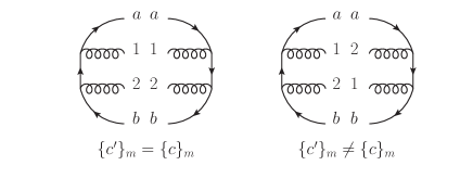
In principle we have to consider diagonal, {c}m={c}msubscriptsuperscript𝑐𝑚subscript𝑐𝑚\{c^{\prime}\}_{m}=\{c\}_{m}, and off-diagonal, {c}m{c}msubscriptsuperscript𝑐𝑚subscript𝑐𝑚\{c^{\prime}\}_{m}\neq\{c\}_{m}, colour configurations, see Fig. 3 for illustration. Notice that the colour diagonal contributions contain the leading colour contribution, while colour off-diagonal contributions are subleading. The latter can be identified by crossing of gluon lines. Traditional parton showers are restricted to the leading colour approximation (or at best to colour diagonal contributions). On the other hand, the Nagy-Soper parton shower allows for the evolution of subleading colour configurations.
Refer to caption
Figure 3: Example colour configurations for the q¯(a)q(b)g(1)g(2)¯𝑞𝑎𝑞𝑏𝑔1𝑔2\bar{q}(a)q(b)g(1)g(2) state.

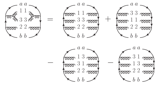
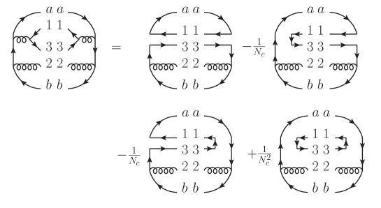
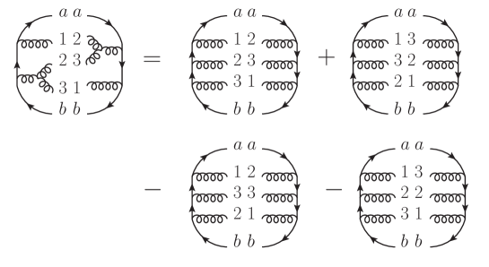
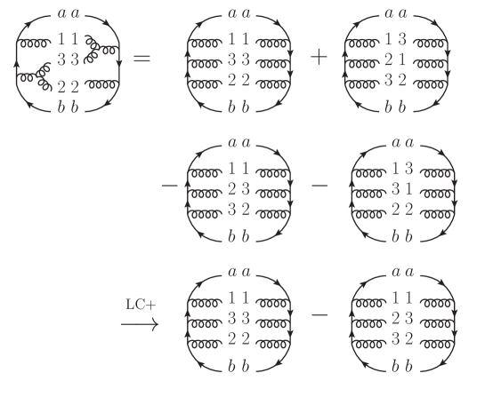
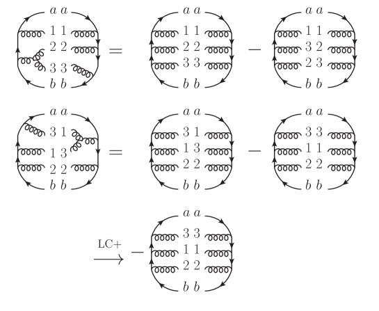
In Figs. 4, 5, 6, 7, and 8, we give several examples of colour evolution induced by direct splitting (application of TlTltensor-productsuperscriptsubscript𝑇𝑙subscript𝑇𝑙T_{l}^{\dagger}\otimes T_{l}) and interference contributions (application of TlTktensor-productsuperscriptsubscript𝑇𝑙subscript𝑇𝑘T_{l}^{\dagger}\otimes T_{k}, where lk𝑙𝑘l\neq k).

Refer to caption
Figure 4: Example of a direct splitting ggg𝑔𝑔𝑔g\to gg starting from a diagonal colour configuration. The left part of the first graph corresponds to l=1𝑙1l=1, while the right part to k=1𝑘1k=1. Moreover, m+1=3𝑚13m+1=3.
Refer to caption
Figure 5: Example of a direct splitting gqq¯𝑔𝑞¯𝑞g\to q\bar{q} starting from a diagonal colour configuration. The left part of the first graph corresponds to l=1𝑙1l=1, while the right part to k=1𝑘1k=1. Moreover, m+1=3𝑚13m+1=3.
Refer to caption
Figure 6: Example of a direct splitting ggg𝑔𝑔𝑔g\to gg starting from an off-diagonal colour configuration. The left part of the first graph corresponds to l=2𝑙2l=2, while the right part to k=2𝑘2k=2. Moreover, m+1=3𝑚13m+1=3.
Refer to caption
Figure 7: Example of an interference contribution of two ggg𝑔𝑔𝑔g\to gg splittings starting from a diagonal colour configuration. The last line represents the LC+ approximation of the original colour structure. The left part of the first graph corresponds to l=2𝑙2l=2, while the right part to k=1𝑘1k=1. Moreover, m+1=3𝑚13m+1=3.
Refer to caption
Figure 8: Example of interference contributions of ggg𝑔𝑔𝑔g\to gg and qqg𝑞𝑞𝑔q\to qg splittings starting from a diagonal colour configuration. Upper graph: the left part of the first graph corresponds to l=2𝑙2l=2, while the right part to k=b𝑘𝑏k=b. Lower graph: the left part of the first graph corresponds to l=a𝑙𝑎l=a, while the right part to k=1𝑘1k=1. Moreover, m+1=3𝑚13m+1=3 in both cases. The last line represents the LC+ approximation of the original colour structure of the lower graph.

The solution of the evolution equation, Eq. (26), requires a decomposition of the virtual operator into a diagonal and an off-diagonal colour part. This can be achieved with the help of the LC+ approximation introduced in Ref. Nagy:2012bt . The main features of this approximation are

  1. 1.

    Exact colour treatment of the collinear and soft-collinear limits;

  2. 2.

    Leading colour approximation for the pure soft limit (a part of the subleading contributions is kept nevertheless).

According to the previous Section, the virtual splitting operator is defined in terms of the real splitting operator. For the latter, the LC+ approximation amounts to the introduction of a projector C(l,m+1)𝐶𝑙𝑚1C(l,m+1) acting on the colour states |{c}m+1ketsubscript𝑐𝑚1\ket{\{c\}_{m+1}} in Eq. (37) as

Tk(fkf^k+f^m+1)|{c}msuperscriptsubscript𝑇𝑘subscript𝑓𝑘subscript^𝑓𝑘subscript^𝑓𝑚1ketsubscript𝑐𝑚\displaystyle T_{k}^{\dagger}(f_{k}\to\hat{f}_{k}+\hat{f}_{m+1})\ket{\{c\}_{m}} C(l,m+1)Tk(fkf^k+f^m+1)|{c}m,absent𝐶𝑙𝑚1superscriptsubscript𝑇𝑘subscript𝑓𝑘subscript^𝑓𝑘subscript^𝑓𝑚1ketsubscript𝑐𝑚\displaystyle\to C(l,m+1)T_{k}^{\dagger}(f_{k}\to\hat{f}_{k}+\hat{f}_{m+1})\ket{\{c\}_{m}}\;, (47)
{c}m|Tk(fkf^k+f^m+1)brasubscriptsuperscript𝑐𝑚subscript𝑇𝑘subscript𝑓𝑘subscript^𝑓𝑘subscript^𝑓𝑚1\displaystyle\bra{\{c^{\prime}\}_{m}}T_{k}(f_{k}\to\hat{f}_{k}+\hat{f}_{m+1}) {c}m|Tk(fkf^k+f^m+1)C(l,m+1),absentbrasubscriptsuperscript𝑐𝑚subscript𝑇𝑘subscript𝑓𝑘subscript^𝑓𝑘subscript^𝑓𝑚1superscript𝐶𝑙𝑚1\displaystyle\to\bra{\{c^{\prime}\}_{m}}T_{k}(f_{k}\to\hat{f}_{k}+\hat{f}_{m+1})C^{\dagger}(l,m+1)\;, (48)

where

C(l,m+1)|{c}m+1={|{c}m+1partons l and m+1 form a qq¯ pair,|{c}m+1partons l and m+1 are colour connected,0otherwise.𝐶𝑙𝑚1ketsubscript𝑐𝑚1casesketsubscript𝑐𝑚1partons l and m+1 form a qq¯ pairketsubscript𝑐𝑚1partons l and m+1 are colour connected0otherwiseC(l,m+1)\ket{\{c\}_{m+1}}=\begin{cases}\ket{\{c\}_{m+1}}&\text{partons $l$ and $m+1$ form a $q\bar{q}$ pair}\;,\\ \ket{\{c\}_{m+1}}&\text{partons $l$ and $m+1$ are colour connected}\;,\\ 0&\text{otherwise}\;.\end{cases} (49)

Colour connected partons are partons, which are direct neighbours on a colour string as defined in Section 2.1. The definition Eq. (49) guarantees that direct splittings are treated exactly. This is also true for the evolution of off-diagonal colour configurations, as depicted in Fig. 6. In other cases, a part of the contributions is removed, as can be seen in Figs. 7 and 8.

The colour projector C(l,m+1)𝐶𝑙𝑚1C(l,m+1) defines a decomposition

I(t)ILC+(t)+ΔI(t).subscript𝐼𝑡superscriptsubscript𝐼limit-from𝐿𝐶𝑡Δsubscript𝐼𝑡\mathcal{H}_{I}(t)\equiv\mathcal{H}_{I}^{LC+}(t)+\Delta\mathcal{H}_{I}(t)\;. (50)

All corrections to the LC+ approximation are of order 𝒪(1/Nc2)𝒪1superscriptsubscript𝑁𝑐2\mathcal{O}(1/N_{c}^{2}) and are treated perturbatively. It turns out that the virtual splitting operator 𝒱LC+(t)superscript𝒱limit-from𝐿𝐶𝑡\mathcal{V}^{LC+}(t) defined in terms of ILC+(t)superscriptsubscript𝐼limit-from𝐿𝐶𝑡\mathcal{H}_{I}^{LC+}(t) is colour diagonal Nagy:2012bt . Therefore, we define

𝒱E(t)𝒱LC+(t),𝒱S(t)Δ𝒱(t)=𝒱(t)𝒱LC+(t).formulae-sequencesubscript𝒱𝐸𝑡superscript𝒱limit-from𝐿𝐶𝑡subscript𝒱𝑆𝑡Δ𝒱𝑡𝒱𝑡superscript𝒱limit-from𝐿𝐶𝑡\mathcal{V}_{E}(t)\equiv\mathcal{V}^{LC+}(t)\;,\qquad\mathcal{V}_{S}(t)\equiv\Delta\mathcal{V}(t)=\mathcal{V}(t)-\mathcal{V}^{LC+}(t)\;. (51)

We can also define an approximate evolution operator

ULC+(t,t0)=NLC+(t,t0)+t0t𝑑τULC+(t,τ)ILC+(τ)NLC+(τ,t0),superscript𝑈limit-from𝐿𝐶𝑡subscript𝑡0superscript𝑁limit-from𝐿𝐶𝑡subscript𝑡0superscriptsubscriptsubscript𝑡0𝑡differential-d𝜏superscript𝑈limit-from𝐿𝐶𝑡𝜏superscriptsubscript𝐼limit-from𝐿𝐶𝜏superscript𝑁limit-from𝐿𝐶𝜏subscript𝑡0U^{LC+}(t,t_{0})=N^{LC+}(t,t_{0})+\int_{t_{0}}^{t}d\tau~{}U^{LC+}(t,\tau)\mathcal{H}_{I}^{LC+}(\tau)N^{LC+}(\tau,t_{0})\;, (52)

where

NLC+(t,t0)=exp(t0t𝑑τ𝒱LC+(τ)).superscript𝑁limit-from𝐿𝐶𝑡subscript𝑡0superscriptsubscriptsubscript𝑡0𝑡differential-d𝜏superscript𝒱limit-from𝐿𝐶𝜏N^{LC+}(t,t_{0})=\exp\left(-\int_{t_{0}}^{t}d\tau~{}\mathcal{V}^{LC+}(\tau)\right)\;. (53)

On the other hand, the exact evolution operator is

U(t,t0)=ULC+(t,t0)+t0t𝑑τU(t,τ)[ΔI(τ)Δ𝒱(τ)]ULC+(τ,t0).𝑈𝑡subscript𝑡0superscript𝑈limit-from𝐿𝐶𝑡subscript𝑡0superscriptsubscriptsubscript𝑡0𝑡differential-d𝜏𝑈𝑡𝜏delimited-[]Δsubscript𝐼𝜏Δ𝒱𝜏superscript𝑈limit-from𝐿𝐶𝜏subscript𝑡0U(t,t_{0})=U^{LC+}(t,t_{0})+\int_{t_{0}}^{t}d\tau~{}U(t,\tau)\left[\Delta\mathcal{H}_{I}(\tau)-\Delta\mathcal{V}(\tau)\right]U^{LC+}(\tau,t_{0})\;. (54)

The practical solution of these equations is described in Ref. Nagy:2012bt . The current implementation of Deductor relies on Eq. (52).

Let us comment on the logarithmic accuracy of the Nagy-Soper parton shower. Consider an observable 𝒪𝒪\mathcal{O}, given by the expansion

𝒪=nc(n,2n)αsnL2n+nc(n,2n1)αsnL2n1+,delimited-⟨⟩𝒪subscript𝑛𝑐𝑛2𝑛superscriptsubscript𝛼𝑠𝑛superscript𝐿2𝑛subscript𝑛𝑐𝑛2𝑛1superscriptsubscript𝛼𝑠𝑛superscript𝐿2𝑛1\langle\mathcal{O}\rangle=\sum_{n}c(n,2n)\alpha_{s}^{n}L^{2n}+\sum_{n}c(n,2n-1)\alpha_{s}^{n}L^{2n-1}+\cdots\;, (55)

where L𝐿L denotes a potentially large logarithm, e.g. L=log(s/pT2)𝐿𝑠superscriptsubscript𝑝𝑇2L=\log(s/p_{T}^{2}), where s𝑠s is the scale of the hard process, and pTsubscript𝑝𝑇p_{T} is the transverse momentum of some final state, for example a pair of oppositely charged leptons from the Drell-Yan process. The evolution operator U(t,t0)𝑈𝑡subscript𝑡0U(t,t_{0}) reproduces the coefficients c(n,2n)𝑐𝑛2𝑛c(n,2n) and c(n,2n1)𝑐𝑛2𝑛1c(n,2n-1) without any approximations in colour. On the other hand, ULC+(t,t0)superscript𝑈limit-from𝐿𝐶𝑡subscript𝑡0U^{LC+}(t,t_{0}) misses part of the c(n,2n1)𝑐𝑛2𝑛1c(n,2n-1) coefficient due to subleading colour contributions from wide angle soft radiation. For this reason, the LC+ approximation is only exact at leading logarithm (LL), see Fig. 9. Inserting a factor of [ΔI(τ)Δ𝒱(τ)]delimited-[]Δsubscript𝐼𝜏Δ𝒱𝜏\left[\Delta\mathcal{H}_{I}(\tau)-\Delta\mathcal{V}(\tau)\right] generates the remaining contribution to the coefficient c(n,2n1)𝑐𝑛2𝑛1c(n,2n-1). In consequence, the evolution operator

U(t,t0)=ULC+(t,t0)+t0t𝑑τULC+(t,τ)[ΔI(τ)Δ𝒱(τ)]ULC+(τ,t0),𝑈𝑡subscript𝑡0superscript𝑈limit-from𝐿𝐶𝑡subscript𝑡0superscriptsubscriptsubscript𝑡0𝑡differential-d𝜏superscript𝑈limit-from𝐿𝐶𝑡𝜏delimited-[]Δsubscript𝐼𝜏Δ𝒱𝜏superscript𝑈limit-from𝐿𝐶𝜏subscript𝑡0U(t,t_{0})=U^{LC+}(t,t_{0})+\int_{t_{0}}^{t}d\tau~{}U^{LC+}(t,\tau)\left[\Delta\mathcal{H}_{I}(\tau)-\Delta\mathcal{V}(\tau)\right]U^{LC+}(\tau,t_{0})\;, (56)

is accurate at next-to-leading logarithm (NLL).

Refer to caption
Figure 9: Illustration of the logarithm counting. One step in the vertical direction is given by an insertion of ULC+superscript𝑈limit-from𝐿𝐶U^{LC+} and a diagonal step is given by an insertion of ΔI(t)Δ𝒱(t)Δsubscript𝐼𝑡Δ𝒱𝑡\Delta\mathcal{H}_{I}(t)-\Delta\mathcal{V}(t). One can see, that two insertions of ΔI(t)Δ𝒱(t)Δsubscript𝐼𝑡Δ𝒱𝑡\Delta\mathcal{H}_{I}(t)-\Delta\mathcal{V}(t) only contributes to the coefficient of αsnL2n2superscriptsubscript𝛼𝑠𝑛superscript𝐿2𝑛2\alpha_{s}^{n}L^{2n-2}.

As pointed out before (see discussion around Eq. (42)), the virtual splitting operator is diagonal in spin. Therefore, spin dependent effects are only induced by the action of I(t)subscript𝐼𝑡\mathcal{H}_{I}(t). It has been proposed in Ref. Nagy:2008eq to include them on top of the spin averaged shower. To this end, we note that the necessary modification in I(t)subscript𝐼𝑡\mathcal{H}_{I}(t), Eq. (37), amounts to the replacement

Φlk({p^,f^}m+1)({s^,s^}m+1|Ylk({p^,f^}m+1)|{s,s}m)Φlk({p^,f^}m+1),subscriptΦ𝑙𝑘subscript^𝑝^𝑓𝑚1subscriptsuperscript^𝑠^𝑠𝑚1subscript𝑌𝑙𝑘subscript^𝑝^𝑓𝑚1subscriptsuperscript𝑠𝑠𝑚subscriptΦ𝑙𝑘subscript^𝑝^𝑓𝑚1\Phi_{lk}(\{\hat{p},\hat{f}\}_{m+1})\;\longrightarrow\;(\{\hat{s}^{\prime},\hat{s}\}_{m+1}|Y_{lk}(\{\hat{p},\hat{f}\}_{m+1})|\{s^{\prime},s\}_{m})\;\Phi_{lk}(\{\hat{p},\hat{f}\}_{m+1})\;, (57)

where

Φlk({p^,f^}m+1)=δkl(1δf^m+1,g)w¯ll({p^,f^}m+1+δklδf^m+1,g[w¯ll({p^,f^}m+1w¯lleikonal](1δkl)δf^m+1,gAlk({p^m+1})w¯lkdipole({p^,f^}m+1),\begin{split}\Phi_{lk}(\{\hat{p},\hat{f}\}_{m+1})&=\delta_{kl}\;\big{(}1-\delta_{\hat{f}_{m+1},g}\big{)}\;\overline{w}_{ll}(\{\hat{p},\hat{f}\}_{m+1}\\ &+\delta_{kl}\;\delta_{\hat{f}_{m+1},g}\;\left[\overline{w}_{ll}(\{\hat{p},\hat{f}\}_{m+1}-\overline{w}_{ll}^{eikonal}\right]\\ &-(1-\delta_{kl})\;\delta_{\hat{f}_{m+1},g}\;A_{lk}(\{\hat{p}_{m+1}\})\;\overline{w}_{lk}^{dipole}(\{\hat{p},\hat{f}\}_{m+1})\;,\end{split} (58)

and Ylk({p^,f^}m+1)subscript𝑌𝑙𝑘subscript^𝑝^𝑓𝑚1Y_{lk}(\{\hat{p},\hat{f}\}_{m+1}) is just the ratio between spin dependent and spin averaged splitting functions, see Ref. Nagy:2008eq .

The parton shower evolution starts with a quantum density matrix

({p,f,s,c,s,c}m|ρ(t0))=({p,f,c,c}m|ρ(t0))({s,s}m|ρs({p,f,c,c}m)),conditionalsubscript𝑝𝑓superscript𝑠superscript𝑐𝑠𝑐𝑚𝜌subscript𝑡0tensor-productconditionalsubscript𝑝𝑓superscript𝑐𝑐𝑚𝜌subscript𝑡0conditionalsubscriptsuperscript𝑠𝑠𝑚superscript𝜌𝑠subscript𝑝𝑓superscript𝑐𝑐𝑚(\{p,f,s^{\prime},c^{\prime},s,c\}_{m}|\rho(t_{0}))=(\{p,f,c^{\prime},c\}_{m}|\rho(t_{0}))\otimes(\{s^{\prime},s\}_{m}|\rho^{s}(\{p,f,c^{\prime},c\}_{m}))\;, (59)

with a factorized spin dependence, |ρs)|\rho^{s}), with respect to the spin averaged quantum density |ρ(t0))|\rho(t_{0})). The latter subsequently undergoes spin averaged evolution. On the other hand, after (nm)𝑛𝑚(n-m) real emission steps

|ρns)=Yln,kn({p^,f^}n)Ylm+2,km+2({p^,f^}m+2)Ylm+1,km+1({p^,f^}m+1)|ρs({p,f,c,c}m)).|\rho^{s}_{n})=Y_{l_{n},k_{n}}(\{\hat{p},\hat{f}\}_{n})\cdots Y_{l_{m+2},k_{m+2}}(\{\hat{p},\hat{f}\}_{m+2})Y_{l_{m+1},k_{m+1}}(\{\hat{p},\hat{f}\}_{m+1})|\rho^{s}(\{p,f,c^{\prime},c\}_{m}))\;. (60)

Assuming that the final observable does not depend on the spin configuration, we obtain

σ[F]=λ1λ![d{p,f,c,c}λ](F|{p,f,c,c}λ)({p,f,c,c}λ|ρ(tF))(1spin|ρλs),𝜎delimited-[]𝐹subscript𝜆1𝜆delimited-[]𝑑subscript𝑝𝑓superscript𝑐𝑐𝜆conditional𝐹subscript𝑝𝑓superscript𝑐𝑐𝜆conditionalsubscript𝑝𝑓superscript𝑐𝑐𝜆𝜌subscript𝑡𝐹conditionalsubscript1𝑠𝑝𝑖𝑛subscriptsuperscript𝜌𝑠𝜆\sigma[F]=\sum_{\lambda}\frac{1}{\lambda!}\int[d\{p,f,c^{\prime},c\}_{\lambda}](F|\{p,f,c^{\prime},c\}_{\lambda})(\{p,f,c^{\prime},c\}_{\lambda}|\rho(t_{F}))(1_{spin}|\rho^{s}_{\lambda})\;, (61)

where

(1spin|ρλs)={s,s}λ(1spin|{s,s}λ)({s,s}λ|ρλs)={s}λ({s,s}λ|ρλs).conditionalsubscript1𝑠𝑝𝑖𝑛subscriptsuperscript𝜌𝑠𝜆subscriptsubscriptsuperscript𝑠𝑠𝜆conditionalsubscript1𝑠𝑝𝑖𝑛subscriptsuperscript𝑠𝑠𝜆conditionalsubscriptsuperscript𝑠𝑠𝜆subscriptsuperscript𝜌𝑠𝜆subscriptsubscript𝑠𝜆conditionalsubscript𝑠𝑠𝜆subscriptsuperscript𝜌𝑠𝜆(1_{spin}|\rho^{s}_{\lambda})=\sum_{\{s^{\prime},s\}_{\lambda}}(1_{spin}|\{s^{\prime},s\}_{\lambda})(\{s^{\prime},s\}_{\lambda}|\rho^{s}_{\lambda})=\sum_{\{s\}_{\lambda}}(\{s,s\}_{\lambda}|\rho^{s}_{\lambda})\;. (62)

2.7 Shower time

The forward evolution in the shower time is used to enforce an ordering in some chosen kinematic variable. This is necessary in order to correctly resum leading logarithms of infrared sensitive quantities. In traditional parton shower programs the following ordering variables are used:

virtuality:

the invariant mass of two daughter partons produced through the splitting (e.g. Pythia6Q Sjostrand:2006za ),

transverse momentum:

the transverse momentum of the daughter partons with respect to the mother parton (e.g. Pythia8 Sjostrand:2007gs ),

angle:

the angle between the momenta of the daughter partons (e.g. Herwig Bahr:2008pv ; Corcella:2000bw ).

The construction of a new parton shower allows to re-evaluate the advantages of these variables, and replace them if necessary. In Ref. Nagy:2014nqa , the following variable has been proposed

Λl2=|(p^l±p^m+1)2ml2|2plQ0Q02,subscriptsuperscriptΛ2𝑙superscriptplus-or-minussubscript^𝑝𝑙subscript^𝑝𝑚12subscriptsuperscript𝑚2𝑙2subscript𝑝𝑙subscript𝑄0superscriptsubscript𝑄02\Lambda^{2}_{l}=\frac{|(\hat{p}_{l}\pm\hat{p}_{m+1})^{2}-m^{2}_{l}|}{2p_{l}\cdot Q_{0}}Q_{0}^{2}\;, (63)

where p^lsubscript^𝑝𝑙\hat{p}_{l} is the emitter momentum after emission (daughter parton), p^m+1subscript^𝑝𝑚1\hat{p}_{m+1} the emitted parton momentum (daughter parton), plsubscript𝑝𝑙p_{l} the emitter momentum before emission (mother parton with mass mlsubscript𝑚𝑙m_{l}) and Q0subscript𝑄0Q_{0} is the total final state momentum. The minus sign between p^lsubscript^𝑝𝑙\hat{p}_{l} and p^m+1subscript^𝑝𝑚1\hat{p}_{m+1} in Eq. (63) applies to an initial state splitting. The shower time with Λl2subscriptsuperscriptΛ2𝑙\Lambda^{2}_{l} ordering is then given by

𝒯l({p,f}m)log(Λl2Q02).subscript𝒯𝑙subscript𝑝𝑓𝑚superscriptsubscriptΛ𝑙2superscriptsubscript𝑄02\mathcal{T}_{l}(\{p,f\}_{m})\equiv-\log\left(\frac{\Lambda_{l}^{2}}{Q_{0}^{2}}\right)\;. (64)

The particular form of Λl2superscriptsubscriptΛ𝑙2\Lambda_{l}^{2} may be justified as follows Nagy:2014nqa . Consider a splitting of a final state parton with momentum p0subscript𝑝0p_{0} into two partons with momenta p1subscript𝑝1p_{1} and p2subscript𝑝2p_{2}. After splitting the mother parton has non-vanishing additional virtuality v02superscriptsubscript𝑣02v_{0}^{2} (=p02m02absentsuperscriptsubscript𝑝02superscriptsubscript𝑚02=p_{0}^{2}-m_{0}^{2}), while both daughter partons are on-shell. In subsequent steps, both daughter partons will split as well, and acquire additional virtualities v12superscriptsubscript𝑣12v_{1}^{2} and v22superscriptsubscript𝑣22v_{2}^{2} (=pi2mi2absentsuperscriptsubscript𝑝𝑖2superscriptsubscript𝑚𝑖2=p_{i}^{2}-m_{i}^{2}). Clearly, v02superscriptsubscript𝑣02v_{0}^{2} will be modified by this procedure. The validity of the on-shell approximation used in the first step necessitates the effect on v02superscriptsubscript𝑣02v_{0}^{2} to be negligible. This can be translated into the following conditions Nagy:2014nqa

v122p1Q0v022p0Q0 and v222p2Q0v022p0Q0.formulae-sequencemuch-less-thansuperscriptsubscript𝑣122subscript𝑝1subscript𝑄0superscriptsubscript𝑣022subscript𝑝0subscript𝑄0 and much-less-thansuperscriptsubscript𝑣222subscript𝑝2subscript𝑄0superscriptsubscript𝑣022subscript𝑝0subscript𝑄0\frac{v_{1}^{2}}{2p_{1}\cdot Q_{0}}\ll\frac{v_{0}^{2}}{2p_{0}\cdot Q_{0}}\quad\text{ and }\quad\frac{v_{2}^{2}}{2p_{2}\cdot Q_{0}}\ll\frac{v_{0}^{2}}{2p_{0}\cdot Q_{0}}\;. (65)

Up to normalization, the terms vl22plQ0superscriptsubscript𝑣𝑙22subscript𝑝𝑙subscript𝑄0\frac{v_{l}^{2}}{2p_{l}\cdot Q_{0}} are equal to Λl2subscriptsuperscriptΛ2𝑙\Lambda^{2}_{l}. A similar discussion holds for the initial state shower. We note that one of the consequences of Λl2superscriptsubscriptΛ𝑙2\Lambda_{l}^{2} ordering is an enlarged phase space for initial state splittings compared to pTsubscript𝑝𝑇p_{T} ordering.

2.8 Consequences of backward evolution

Initial state splittings are generated by the backward evolution formalism first introduced by Sjöstrand in Refs. Sjostrand:1985xi ; Bengtsson:1986gz . In this approach, the Sudakov form factor contains a ratio of parton distribution functions to guide the evolution of the momentum fraction during splitting. Nevertheless, as long as mass effects are neglected and the splitting functions used in the shower and PDF evolution are the same, one can factor out the non-perturbative part completely. This matches the treatment of final state radiation, where hadronization only happens after showering. Unfortunately, the splitting functions used in the Nagy-Soper parton shower are very different from those of Altarelli-Parisi away from the collinear limit. Thus, non-perturbative information will inevitably affect the evolution.

In the presence of mass effects, however, the non-perturbative input can not be factorized, independently of the approach to the parton shower (traditional or otherwise), unless the evolution of PDFs is modified. We describe the required modification after Ref. Nagy:2014oqa , which has been implemented in Deductor.

In principle we would like to decompose the density matrix as

|ρ)=(t)|ρpert),|\rho)=\mathcal{L}(t)|\rho_{\text{pert}})\;, (66)

where |ρpert)|\rho_{\text{pert}}) would contain no non-perturbative information if splittings were restricted to the quasi-collinear limit. Here, the luminosity operator (t)𝑡\mathcal{L}(t) is

(t)|Φm)fa/A(ηa,μA2et)fb/B(ηb,μB2et)4nc(a)nc(b)4ηaηbpApB|Φm),\mathcal{L}(t)|\Phi_{m})\equiv\frac{f_{a/A}(\eta_{a},\mu_{A}^{2}e^{-t})f_{b/B}(\eta_{b},\mu_{B}^{2}e^{-t})}{4n_{c}(a)n_{c}(b)4\eta_{a}\eta_{b}p_{A}\cdot p_{B}}|\Phi_{m})\;, (67)

where we used a shorthand notation for the statistical states, Φλ={p,f,s,c,s,c}λsubscriptΦ𝜆subscript𝑝𝑓superscript𝑠superscript𝑐𝑠𝑐𝜆\Phi_{\lambda}=\{p,f,s^{\prime},c^{\prime},s,c\}_{\lambda}. The scale μi2superscriptsubscript𝜇𝑖2\mu_{i}^{2} is given by μi2=2piQ0superscriptsubscript𝜇𝑖22subscript𝑝𝑖subscript𝑄0\mu_{i}^{2}=2p_{i}\cdot Q_{0}, where pisubscript𝑝𝑖p_{i} are the hadron momenta and Q0subscript𝑄0Q_{0} the total final state momentum. Therefore, the PDFs are evaluated at the scale μi2et=|(p^ip^m+1)2mi2|superscriptsubscript𝜇𝑖2superscript𝑒𝑡superscriptsubscript^𝑝𝑖subscript^𝑝𝑚12superscriptsubscript𝑚𝑖2\mu_{i}^{2}e^{-t}=|(\hat{p}_{i}-\hat{p}_{m+1})^{2}-m_{i}^{2}| which is the virtuality of the splitting. Let us define a perturbative real splitting operator, Ipert(t)superscriptsubscript𝐼pert𝑡\mathcal{H}_{I}^{\text{pert}}(t), through

I(t)=(t)Ipert(t)1(t).subscript𝐼𝑡𝑡superscriptsubscript𝐼pert𝑡superscript1𝑡\mathcal{H}_{I}(t)=\mathcal{L}(t)\mathcal{H}_{I}^{\text{pert}}(t)\mathcal{L}^{-1}(t)\;. (68)

Unfortunately, 𝒱(t)𝒱𝑡\mathcal{V}(t) contains a convolution of splitting functions with PDFs, because it is an integral of Eq. (68). It is thus impossible to trivially factor out the non-perturbative contribution. Nevertheless, we can define a quasi-perturbative virtual splitting operator, 𝒱pert(t)superscript𝒱pert𝑡\mathcal{V}^{\text{pert}}(t), via the evolution equation. Indeed, substituting Eq. (66) in Eq. (22) we obtain

(ddt(t))|ρpert)+(t)(ddt|ρpert))=[I(t)𝒱(t)](t)|ρpert).\left(\frac{d}{dt}\mathcal{L}(t)\right)|\rho_{\text{pert}})+\mathcal{L}(t)\left(\frac{d}{dt}|\rho_{\text{pert}})\right)=\left[\mathcal{H}_{I}(t)-\mathcal{V}(t)\right]\mathcal{L}(t)|\rho_{\text{pert}})\;. (69)

This allows us to write

ddt|ρpert)=[Ipert(t)𝒱pert(t)]|ρpert),\frac{d}{dt}|\rho_{\text{pert}})=\left[\mathcal{H}_{I}^{\text{pert}}(t)-\mathcal{V}^{\text{pert}}(t)\right]|\rho_{\text{pert}})\;, (70)

with

𝒱pert(t)=𝒱(t)+1(t)(ddt(t)),superscript𝒱pert𝑡𝒱𝑡superscript1𝑡𝑑𝑑𝑡𝑡\mathcal{V}^{\text{pert}}(t)=\mathcal{V}(t)+\mathcal{L}^{-1}(t)\left(\frac{d}{dt}\mathcal{L}(t)\right)\;, (71)

where we used the fact that (t)𝑡\mathcal{L}(t) commutes with 𝒱(t)𝒱𝑡\mathcal{V}(t) since it does not change the momenta.

To ensure that 𝒱pert(t)superscript𝒱pert𝑡\mathcal{V}^{\text{pert}}(t) is independent of PDFs in the quasi-collinear limit, the splitting functions obtained by deriving (t)𝑡\mathcal{L}(t) must match the quasi-collinear limit of 𝒱(t)𝒱𝑡\mathcal{V}(t). The respective functions are given in Ref. Nagy:2014oqa . As expected, they only differ from the Altarelli-Parisi kernels at non-zero mass. They also imply a modified evolution of the PDFs. The effect is mostly visible on the b𝑏b-quark PDF. Clearly, only processes predominantly generated from initial state b𝑏b-quarks will be influenced.

Modifying the evolution of parton distribution functions may be used for other purposes as well. For instance, adding a higher order term Paa^(2)subscriptsuperscript𝑃2𝑎^𝑎P^{(2)}_{a\hat{a}} as follows

dfa/A(ηa,μ2)dlog(μ2)=a^dzzαs(μ2/z)2πPaa^(z,μ2/z)fa^/A(ηa/z,μ2)+a^dzz(αs(μ2/z)2π)2Paa^(2)(z,μ2/z)fa^/A(ηa/z,μ2),𝑑subscript𝑓𝑎𝐴subscript𝜂𝑎superscript𝜇2𝑑superscript𝜇2subscript^𝑎𝑑𝑧𝑧subscript𝛼𝑠superscript𝜇2𝑧2𝜋subscript𝑃𝑎^𝑎𝑧superscript𝜇2𝑧subscript𝑓^𝑎𝐴subscript𝜂𝑎𝑧superscript𝜇2subscript^𝑎𝑑𝑧𝑧superscriptsubscript𝛼𝑠superscript𝜇2𝑧2𝜋2subscriptsuperscript𝑃2𝑎^𝑎𝑧superscript𝜇2𝑧subscript𝑓^𝑎𝐴subscript𝜂𝑎𝑧superscript𝜇2\begin{split}\frac{df_{a/A}(\eta_{a},\mu^{2})}{d\log(\mu^{2})}&=\sum_{\hat{a}}\int\frac{dz}{z}\frac{\alpha_{s}(\mu^{2}/z)}{2\pi}P_{a\hat{a}}(z,\mu^{2}/z)f_{\hat{a}/A}(\eta_{a}/z,\mu^{2})\\ &+\sum_{\hat{a}}\int\frac{dz}{z}\left(\frac{\alpha_{s}(\mu^{2}/z)}{2\pi}\right)^{2}P^{(2)}_{a\hat{a}}(z,\mu^{2}/z)f_{\hat{a}/A}(\eta_{a}/z,\mu^{2})\;,\end{split} (72)

with

Paa^(2)(z,μ2/z)=2πβ0log(λR)Paa^(z,μ2/z),subscriptsuperscript𝑃2𝑎^𝑎𝑧superscript𝜇2𝑧2𝜋subscript𝛽0subscript𝜆𝑅subscript𝑃𝑎^𝑎𝑧superscript𝜇2𝑧P^{(2)}_{a\hat{a}}(z,\mu^{2}/z)=-2\pi\beta_{0}\log(\lambda_{R})P_{a\hat{a}}(z,\mu^{2}/z)\;, (73)

where β0=(332nf)/(12π)subscript𝛽0332subscript𝑛𝑓12𝜋\beta_{0}=(33-2n_{f})/(12\pi) and

λR=exp(CA(673π2)10nf3(332nf)),subscript𝜆𝑅subscript𝐶𝐴673superscript𝜋210subscript𝑛𝑓3332subscript𝑛𝑓\lambda_{R}=\exp\left(-\frac{C_{A}(67-3\pi^{2})-10n_{f}}{3(33-2n_{f})}\right)\;, (74)

where nfsubscript𝑛𝑓n_{f} is the number of light active flavours, allows to incorporate the cusp anomalous dimension at NLL for processes with less then three coloured particles Catani:1990rr .

2.9 A summary of ambiguities

Let us conclude this Section with a list of ambiguous components of the Nagy-Soper parton shower:

  1. 1.

    Momentum Mappings

  2. 2.

    Splitting functions

  3. 3.

    Soft partition function

  4. 4.

    Colour treatment

  5. 5.

    Spin treatment

  6. 6.

    Shower time

  7. 7.

    PDF evolution

We stress that this shower is a rather recent construction still under development. It is to be expected that there will be changes to any of the particular solutions discussed in the previous Subsections.

3 Matching NLO matrix elements to the parton shower

Matching NLO calculations with parton showers is a widely explored subject and there exist several matching schemes, the most popular being Powheg Nason:2004rx ; Frixione:2007vw and Mc@Nlo Frixione:2002ik ; Frixione:2003ei (for other proposals see e.g. Kramer:2003jk ; Soper:2003ya ; Kramer:2005hw ; Nagy:2005aa ; Giele:2007di ; Torrielli:2010aw ; Hoche:2010pf ; Platzer:2011bc ; Hartgring:2013jma ). A general comparison between these two can be found in e.g. Hoeche:2011fd . In order to benefit from the recently implemented subtraction scheme based on the Nagy-Soper parton shower splitting kernels Bevilacqua:2013iha , we chose the Mc@Nlo formalism. Notice, that the implementation of Mc@Nlo in Sherpa Hoeche:2011fd also benefits from the consistency between the parton shower (Catani-Seymour) and subtraction terms in the matching. However, once the implementation of the Nagy-Soper parton shower will be made accurate at subleading terms in the colour expansion, our matching procedure will allow for a similar accuracy in the matched sample. This may also be possible in the future within Sherpa, see Ref. Platzer:2012np . Before we discuss the challenges of parton shower matching, we give a brief overview of the general objectives.

Preserving the NLO cross section normalization: When considering an inclusive observable F𝐹F, the fixed order normalization of the cross section should be preserved. We thus require

(F|U(tF,t0)|ρ(t0))=σNLO[F].𝐹𝑈subscript𝑡𝐹subscript𝑡0𝜌subscript𝑡0superscript𝜎𝑁𝐿𝑂delimited-[]𝐹(F|U(t_{F},t_{0})|\rho(t_{0}))=\sigma^{NLO}[F]\;. (75)

Defining event samples at NLO level: Matching to parton shower is the only way to define events at NLO. As we will see, matching à la Mc@Nlo imposes a shower specific subtraction scheme. Without matching, the weights of the real matrix element and the subtraction terms are not coupled kinematically unless in a strict limit, and diverge separately. Due to the matching scheme those weights are combined and one obtains real emission phase space configurations with a finite, but not necessarily positive, weight. The matching renders the virtual corrections finite as well.

Next-to-Leading Logarithmic accuracy for infrared sensitive observables: Infrared sensitive observables, which are affected by large logarithms, L𝐿L, of some kinematic variable at fixed-order, are replaced by resummed predictions. Traditional parton showers only resum the leading logarithms (LL) αsnL2nsuperscriptsubscript𝛼𝑠𝑛superscript𝐿2𝑛\alpha_{s}^{n}L^{2n}, whereas the Nagy-Soper shower also allows to resum the next-to-leading logarithms (NLL) αsnL2n1superscriptsubscript𝛼𝑠𝑛superscript𝐿2𝑛1\alpha_{s}^{n}L^{2n-1}. Therefore, we require differential distributions to be accurate at the NLO++NLL level.

High pTsubscript𝑝𝑇p_{T} emissions according to matrix elements: The parton shower is valid in the soft and collinear regimes, the description of high pTsubscript𝑝𝑇p_{T} emissions is, therefore, not reliable. On the other hand, NLO calculations are valid in this region. It is desirable to recover the NLO prediction for high pTsubscript𝑝𝑇p_{T} emissions despite applying the parton shower.

Connection to low energy physics: The parton evolution down to a low scale allows to include non-perturbative phenomena due to hadronization and multiple interactions.

3.1 The quantum density matrix at next-to-leading order

For a generic 2m2𝑚2\to m process at NLO, one can write the quantum density matrix in a perturbative expansion in αssubscript𝛼𝑠\alpha_{s}, according to

|ρ)=|ρm(0))Born,𝒪(1)+|ρm(1))Virtual,𝒪(αs)+|ρm+1(0))Real,𝒪(αs)+𝒪(αs2).|\rho)=\underbrace{|\rho_{m}^{(0)})}_{\text{Born},\;\mathcal{O}(1)}+\underbrace{|\rho_{m}^{(1)})}_{\text{Virtual},\;\mathcal{O}(\alpha_{s})}+\underbrace{|\rho_{m+1}^{(0)})}_{\text{Real},\;\mathcal{O}(\alpha_{s})}+\mathcal{O}(\alpha_{s}^{2})\;. (76)

Note that we count the leading order contribution as order 111 in the strong coupling αssubscript𝛼𝑠\alpha_{s}. |ρm(0))|\rho_{m}^{(0)}) and |ρm+1(0))|\rho_{m+1}^{(0)}) are tree level matrix elements, whereas |ρm(1))|\rho_{m}^{(1)}) is the one-loop amplitude. The definitions of these densities are analogous to the definition given in Eq. (12). So far Eq. (76) suffers from infrared divergences, however, the expansion of |ρ)|\rho) in αssubscript𝛼𝑠\alpha_{s} is defined within dimensional regularization. Based on this quantum density matrix, the expectation value of the observable F𝐹F including shower effects reads

σ[F]PS=(F|U(tF,t0)|ρ)=λ=m1λ![dΦλ](F|Φλ)(Φλ|U(tF,t0)|ρ),𝜎superscriptdelimited-[]𝐹𝑃𝑆𝐹𝑈subscript𝑡𝐹subscript𝑡0𝜌superscriptsubscript𝜆𝑚1𝜆delimited-[]𝑑subscriptΦ𝜆conditional𝐹subscriptΦ𝜆subscriptΦ𝜆𝑈subscript𝑡𝐹subscript𝑡0𝜌\sigma[F]^{PS}=(F|U(t_{F},t_{0})|\rho)=\sum_{\lambda=m}^{\infty}\frac{1}{\lambda!}\int[d\Phi_{\lambda}](F|\Phi_{\lambda})(\Phi_{\lambda}|U(t_{F},t_{0})|\rho)\;, (77)

where Φλ={p,f,s,c,s,c}λsubscriptΦ𝜆subscript𝑝𝑓superscript𝑠superscript𝑐𝑠𝑐𝜆\Phi_{\lambda}=\{p,f,s^{\prime},c^{\prime},s,c\}_{\lambda}. The quantum density |ρ)|\rho) accounts for the hard matrix elements for λ=m𝜆𝑚\lambda=m and λ=m+1𝜆𝑚1\lambda=m+1. This naive description of the cross section suffers from double counting, as we will show using the iterative solution to the evolution equation expanded to 𝒪(αs)𝒪subscript𝛼𝑠\mathcal{O}(\alpha_{s}). Indeed, there is

|ρ(tF))=U(tF,t0)|ρ)|ρ)+t0tFdτ[I(τ)𝒱(τ)]|ρm(0))+𝒪(αs2).|\rho(t_{F}))=U(t_{F},t_{0})|\rho)\approx|\rho)+\int_{t_{0}}^{t_{F}}d\tau\left[\mathcal{H}_{I}(\tau)-\mathcal{V}(\tau)\right]|\rho_{m}^{(0)})+\mathcal{O}(\alpha_{s}^{2})\;. (78)

As we can see from the unitarity condition (1|[I(τ)𝒱(τ)]=0(1|\left[\mathcal{H}_{I}(\tau)-\mathcal{V}(\tau)\right]=0, the total cross section (1|ρ(tF))conditional1𝜌subscript𝑡𝐹(1|\rho(t_{F})) is conserved. On the other hand, one does not recover the NLO prediction for inclusive observables F𝐹F because in general (F|[I(τ)𝒱(τ)]0(F|\left[\mathcal{H}_{I}(\tau)-\mathcal{V}(\tau)\right]\neq 0. Even without this requirement the result is not correct, since it contains the first emission contributions twice, once from the real emission quantum density |ρm+1(0))|\rho^{(0)}_{m+1}), and once from the parton shower approximation I(τ)|ρm(0))\mathcal{H}_{I}(\tau)|\rho^{(0)}_{m}). We will now show how to overcome this problem.

3.2 Matching fully inclusive processes to parton shower

Let us begin with a class of processes, which have a well defined total cross section at leading order, e.g. pptt¯𝑝𝑝𝑡¯𝑡pp\to t\bar{t} or ppW+W𝑝𝑝superscript𝑊superscript𝑊pp\to W^{+}W^{-}. Working along the line of the Mc@Nlo scheme, we notice that the additional parton shower contribution in Eq. (78) can be cancelled by including appropriate counterterms. Let us, therefore, introduce the following modified quantum density matrix

|ρ¯)|ρ)t0tFdτ[I(τ)𝒱(τ)]|ρm(0))+𝒪(αs2).|\bar{\rho})\equiv|\rho)-\int_{t_{0}}^{t_{F}}d\tau\left[\mathcal{H}_{I}(\tau)-\mathcal{V}(\tau)\right]|\rho_{m}^{(0)})+\mathcal{O}(\alpha_{s}^{2})\;. (79)

The total cross section (1|ρ¯)=(1|ρ)=σNLOconditional1¯𝜌conditional1𝜌superscript𝜎𝑁𝐿𝑂(1|\bar{\rho})=(1|\rho)=\sigma^{NLO} is unchanged, due to the unitarity condition. On the other hand, considering U(tF,t0)|ρ¯)U(t_{F},t_{0})|\bar{\rho}) and expanding the evolution equation shows that the undesired parton shower contributions are cancelled up to 𝒪(αs)𝒪subscript𝛼𝑠\mathcal{O}(\alpha_{s}). This cancellation is non-trivial, because the modified quantum density matrix |ρ¯)|\bar{\rho}), now depends explicitly on the parton shower splitting kernels, the momentum mappings, the ordering of the emissions and the choice of the starting shower time t0subscript𝑡0t_{0}.

For an infrared safe observable F𝐹F, we have

σ¯[F]=1m![dΦm](F|U(tF,t0)|Φm)[(Φm|ρm(0))+(Φm|ρm(1))+t0tF𝑑τ(Φm|𝒱(τ)|ρm(0))]+1(m+1)![dΦm+1](F|U(tF,t0)|Φm+1)[(Φm+1|ρm+1(0))t0tF𝑑τ(Φm+1|I(τ)|ρm(0))].¯𝜎delimited-[]𝐹1𝑚delimited-[]𝑑subscriptΦ𝑚𝐹𝑈subscript𝑡𝐹subscript𝑡0subscriptΦ𝑚delimited-[]conditionalsubscriptΦ𝑚superscriptsubscript𝜌𝑚0conditionalsubscriptΦ𝑚superscriptsubscript𝜌𝑚1superscriptsubscriptsubscript𝑡0subscript𝑡𝐹differential-d𝜏subscriptΦ𝑚𝒱𝜏superscriptsubscript𝜌𝑚01𝑚1delimited-[]𝑑subscriptΦ𝑚1𝐹𝑈subscript𝑡𝐹subscript𝑡0subscriptΦ𝑚1delimited-[]conditionalsubscriptΦ𝑚1superscriptsubscript𝜌𝑚10superscriptsubscriptsubscript𝑡0subscript𝑡𝐹differential-d𝜏subscriptΦ𝑚1subscript𝐼𝜏superscriptsubscript𝜌𝑚0\begin{split}\bar{\sigma}[F]&=\frac{1}{m!}\int[d\Phi_{m}](F|U(t_{F},t_{0})|\Phi_{m})\left[(\Phi_{m}|\rho_{m}^{(0)})+(\Phi_{m}|\rho_{m}^{(1)})+\int_{t_{0}}^{t_{F}}d\tau(\Phi_{m}|\mathcal{V}(\tau)|\rho_{m}^{(0)})\right]\\ &+\frac{1}{(m+1)!}\int[d\Phi_{m+1}](F|U(t_{F},t_{0})|\Phi_{m+1})\left[(\Phi_{m+1}|\rho_{m+1}^{(0)})-\int_{t_{0}}^{t_{F}}d\tau(\Phi_{m+1}|\mathcal{H}_{I}(\tau)|\rho_{m}^{(0)})\right]\;.\end{split} (80)

In the Mc@Nlo approach, the parton shower splitting kernels are used to provide subtraction terms for the infrared divergences in |ρm(1))|\rho^{(1)}_{m}) and |ρm+1(0))|\rho^{(0)}_{m+1}). Thus, the infrared cutoff tFsubscript𝑡𝐹t_{F} may be removed by taking the limit tFsubscript𝑡𝐹t_{F}\to\infty. Even though this is a source of a mismatch between the fixed order and the shower calculation, it is numerically small due to the exponential damping by the Sudakov form factor as discussed in Ref. Sjostrand:1985xi . In the real subtracted cross section, described in the second line of Eq. (80), we use the definition of the real splitting operator from Eq. (36) and write

t0𝑑τI(τ)=l𝐒l0𝑑τδ(τtl)Θ(τt0)=l𝐒lΘ(tlt0).superscriptsubscriptsubscript𝑡0differential-d𝜏subscript𝐼𝜏subscript𝑙subscript𝐒𝑙superscriptsubscript0differential-d𝜏𝛿𝜏subscript𝑡𝑙Θ𝜏subscript𝑡0subscript𝑙subscript𝐒𝑙Θsubscript𝑡𝑙subscript𝑡0\int_{t_{0}}^{\infty}d\tau~{}\mathcal{H}_{I}(\tau)=\sum_{l}\mathbf{S}_{l}\int_{0}^{\infty}d\tau~{}\delta(\tau-t_{l})\Theta(\tau-t_{0})=\sum_{l}\mathbf{S}_{l}\Theta(t_{l}-t_{0})\;. (81)

Here the sum runs over all external legs and 𝐒lsubscript𝐒𝑙\mathbf{S}_{l} is the total splitting kernel for a given external leg l𝑙l. We want to emphasize that 𝐒lsubscript𝐒𝑙\mathbf{S}_{l} also contains non-singular contributions like the massive gQQ¯𝑔𝑄¯𝑄g\to Q\bar{Q} splitting. Therefore, the operator I(t)subscript𝐼𝑡\mathcal{H}_{I}(t) contains more than is needed for a subtraction scheme. The parameter tlsubscript𝑡𝑙t_{l} is the shower time defined in Section 2.7. Hence, Θ(tlt0)Θsubscript𝑡𝑙subscript𝑡0\Theta(t_{l}-t_{0}) represents the ordering of the emissions and the t0subscript𝑡0t_{0} dependence introduces a dynamical restriction of the subtraction phase space. The choice of t0subscript𝑡0t_{0} will be discussed at the end of this chapter, because it has non-trivial consequences. The real subtracted cross section is finite in d=4𝑑4d=4 dimensions, as tlsubscript𝑡𝑙t_{l} is allowed to approach infinity.

Integrating the virtual operator 𝒱(τ)𝒱𝜏\mathcal{V}(\tau) without an infrared cutoff is more complex, considering that there is an explicit integration over the splitting variables. Hence, we have to integrate this part in d=42ϵ𝑑42italic-ϵd=4-2\epsilon dimensions analytically to extract the 1/ϵ21superscriptitalic-ϵ21/\epsilon^{2} and 1/ϵ1italic-ϵ1/\epsilon poles. The integrated virtual operator takes the form

t0𝑑τ𝒱(τ)=l𝑑Γl𝐒lΘ(tlt0)𝐈(t0)+𝐊(t0),superscriptsubscriptsubscript𝑡0differential-d𝜏𝒱𝜏subscript𝑙differential-dsubscriptΓ𝑙subscript𝐒𝑙Θsubscript𝑡𝑙subscript𝑡0𝐈subscript𝑡0𝐊subscript𝑡0\int_{t_{0}}^{\infty}d\tau~{}\mathcal{V}(\tau)=\sum_{l}\int d\Gamma_{l}\;\mathbf{S}_{l}\Theta(t_{l}-t_{0})\equiv\mathbf{I}(t_{0})+\mathbf{K}(t_{0})\;, (82)

where dΓl𝑑subscriptΓ𝑙d\Gamma_{l} is the phase space integration of the additional parton. The decomposition of the integrated 𝒱(τ)𝒱𝜏\mathcal{V}(\tau) into two operators 𝐈(t0)𝐈subscript𝑡0\mathbf{I}(t_{0}) and 𝐊(t0)𝐊subscript𝑡0\mathbf{K}(t_{0}) is arbitrary. However, we choose 𝐈(t0)𝐈subscript𝑡0\mathbf{I}(t_{0}) to match the divergencies of the virtual amplitude, as it is customary. We emphasize this structure to illustrate that the parton shower naturally incorporates a subtraction scheme similar to the Catani-Seymour framework Catani:1996vz ; Catani:2002hc . In the case of initial state partons it is necessary to include additional collinear counterterms, denoted by 𝐏𝐏\mathbf{P}, needed for the renormalization of the parton distribution functions. Thus, the matched cross section reads

σ¯[F]=[dΦm]m!(F|U(tF,t0)|Φm)[(Φm|ρm(0))+(Φm|ρm(1))+(Φm|[𝐈(t0)+𝐊(t0)+𝐏]|ρm(0))]+[dΦm+1](m+1)!(F|U(tF,t0)|Φm+1)[(Φm+1|ρm+1(0))l(Φm+1|𝐒l|ρm(0))Θ(tlt0)].¯𝜎delimited-[]𝐹delimited-[]𝑑subscriptΦ𝑚𝑚𝐹𝑈subscript𝑡𝐹subscript𝑡0subscriptΦ𝑚delimited-[]conditionalsubscriptΦ𝑚superscriptsubscript𝜌𝑚0conditionalsubscriptΦ𝑚superscriptsubscript𝜌𝑚1subscriptΦ𝑚delimited-[]𝐈subscript𝑡0𝐊subscript𝑡0𝐏superscriptsubscript𝜌𝑚0delimited-[]𝑑subscriptΦ𝑚1𝑚1𝐹𝑈subscript𝑡𝐹subscript𝑡0subscriptΦ𝑚1delimited-[]conditionalsubscriptΦ𝑚1superscriptsubscript𝜌𝑚10subscript𝑙subscriptΦ𝑚1subscript𝐒𝑙superscriptsubscript𝜌𝑚0Θsubscript𝑡𝑙subscript𝑡0\begin{split}\bar{\sigma}[F]&=\int\frac{[d\Phi_{m}]}{m!}(F|U(t_{F},t_{0})|\Phi_{m})\left[(\Phi_{m}|\rho_{m}^{(0)})+(\Phi_{m}|\rho_{m}^{(1)})+(\Phi_{m}|[\mathbf{I}(t_{0})+\mathbf{K}(t_{0})+\mathbf{P}]|\rho_{m}^{(0)})\right]\\ &+\int\frac{[d\Phi_{m+1}]}{(m+1)!}(F|U(t_{F},t_{0})|\Phi_{m+1})\left[(\Phi_{m+1}|\rho_{m+1}^{(0)})-\sum_{l}(\Phi_{m+1}|\mathbf{S}_{l}|\rho_{m}^{(0)})\Theta(t_{l}-t_{0})\right]\;.\end{split} (83)

For future reference, let us define the shorthands, as in Ref. Frixione:2002ik :

(Φm|S)(Φm|ρm(0))+(Φm|ρm(1))+(Φm|[𝐈(t0)+𝐊(t0)+𝐏]|ρm(0)),conditionalsubscriptΦ𝑚𝑆conditionalsubscriptΦ𝑚superscriptsubscript𝜌𝑚0conditionalsubscriptΦ𝑚superscriptsubscript𝜌𝑚1subscriptΦ𝑚delimited-[]𝐈subscript𝑡0𝐊subscript𝑡0𝐏superscriptsubscript𝜌𝑚0\displaystyle(\Phi_{m}|S)\equiv(\Phi_{m}|\rho_{m}^{(0)})+(\Phi_{m}|\rho_{m}^{(1)})+(\Phi_{m}|[\mathbf{I}(t_{0})+\mathbf{K}(t_{0})+\mathbf{P}]|\rho_{m}^{(0)})\;, (84)
(Φm+1|H)(Φm+1|ρm+1(0))l(Φm+1|𝐒l|ρm(0))Θ(tlt0).conditionalsubscriptΦ𝑚1𝐻conditionalsubscriptΦ𝑚1superscriptsubscript𝜌𝑚10subscript𝑙subscriptΦ𝑚1subscript𝐒𝑙superscriptsubscript𝜌𝑚0Θsubscript𝑡𝑙subscript𝑡0\displaystyle(\Phi_{m+1}|H)\equiv(\Phi_{m+1}|\rho_{m+1}^{(0)})-\sum_{l}(\Phi_{m+1}|\mathbf{S}_{l}|\rho_{m}^{(0)})\Theta(t_{l}-t_{0})\;. (85)

The total cross section is then given by

σ¯NLO[1]=1m![dΦm](1|Φm)(Φm|S)+1(m+1)![dΦm+1](1|Φm+1)(Φm+1|H),superscript¯𝜎𝑁𝐿𝑂delimited-[]11𝑚delimited-[]𝑑subscriptΦ𝑚conditional1subscriptΦ𝑚conditionalsubscriptΦ𝑚𝑆1𝑚1delimited-[]𝑑subscriptΦ𝑚1conditional1subscriptΦ𝑚1conditionalsubscriptΦ𝑚1𝐻\bar{\sigma}^{NLO}[1]=\frac{1}{m!}\int[d\Phi_{m}](1|\Phi_{m})(\Phi_{m}|S)+\frac{1}{(m+1)!}\int[d\Phi_{m+1}](1|\Phi_{m+1})(\Phi_{m+1}|H)\;, (86)

whereas including parton shower evolution amounts to the integrals

σ¯[F]PS=1m![dΦm](F|U(tF,t0)|Φm)(Φm|S)+1(m+1)![dΦm+1](F|U(tF,t0)|Φm+1)(Φm+1|H).¯𝜎superscriptdelimited-[]𝐹𝑃𝑆1𝑚delimited-[]𝑑subscriptΦ𝑚𝐹𝑈subscript𝑡𝐹subscript𝑡0subscriptΦ𝑚conditionalsubscriptΦ𝑚𝑆1𝑚1delimited-[]𝑑subscriptΦ𝑚1𝐹𝑈subscript𝑡𝐹subscript𝑡0subscriptΦ𝑚1conditionalsubscriptΦ𝑚1𝐻\begin{split}\bar{\sigma}[F]^{PS}&=\frac{1}{m!}\int[d\Phi_{m}](F|U(t_{F},t_{0})|\Phi_{m})(\Phi_{m}|S)\\ &+\frac{1}{(m+1)!}\int[d\Phi_{m+1}](F|U(t_{F},t_{0})|\Phi_{m+1})(\Phi_{m+1}|H)\;.\end{split} (87)

Matching is a two step procedure, which consists of first generating the samples according to Eq. (84) and (85), followed by the application of U(tF,t0)𝑈subscript𝑡𝐹subscript𝑡0U(t_{F},t_{0}).

3.3 Matching in the presence of singularities in the born approximation

For processes with massless partons at leading order, the matching prescription as described in Eq. (83) must be slightly modified by the inclusion of generation cuts, as discussed for example in Refs. Frederix:2011ig ; Alwall:2014hca . A naive modification to the matching prescription would be to make the following replacements

(Φm|S)conditionalsubscriptΦ𝑚𝑆\displaystyle(\Phi_{m}|S) (Φm|S)FI({p^,f^}m),absentconditionalsubscriptΦ𝑚𝑆subscript𝐹𝐼subscript^𝑝^𝑓𝑚\displaystyle\to(\Phi_{m}|S)F_{I}(\{\hat{p},\hat{f}\}_{m})\;, (88)
(Φm+1|H)conditionalsubscriptΦ𝑚1𝐻\displaystyle(\Phi_{m+1}|H) (Φm+1|H)FI({p,f}m+1),absentconditionalsubscriptΦ𝑚1𝐻subscript𝐹𝐼subscript𝑝𝑓𝑚1\displaystyle\to(\Phi_{m+1}|H)F_{I}(\{p,f\}_{m+1})\;, (89)

where FI({p,f}λ)subscript𝐹𝐼subscript𝑝𝑓𝜆F_{I}(\{p,f\}_{\lambda}) is a jet function applied during the generation of events, on the momenta and flavours of ΦλsubscriptΦ𝜆\Phi_{\lambda}. Applying the parton shower to these ensembles shows that double counting is not removed. Indeed, substituting Eq. (88) and Eq. (89) in Eq. (87) we obtain

σ¯[F]PS=1m![dΦm](F|U(tF,t0)|Φm)(Φm|S)FI({p^,f^}m)+1(m+1)![dΦm+1](F|U(tF,t0)|Φm+1)(Φm+1|H)FI({p,f}m+1).¯𝜎superscriptdelimited-[]𝐹𝑃𝑆1𝑚delimited-[]𝑑subscriptΦ𝑚𝐹𝑈subscript𝑡𝐹subscript𝑡0subscriptΦ𝑚conditionalsubscriptΦ𝑚𝑆subscript𝐹𝐼subscript^𝑝^𝑓𝑚1𝑚1delimited-[]𝑑subscriptΦ𝑚1𝐹𝑈subscript𝑡𝐹subscript𝑡0subscriptΦ𝑚1conditionalsubscriptΦ𝑚1𝐻subscript𝐹𝐼subscript𝑝𝑓𝑚1\begin{split}\bar{\sigma}[F]^{PS}&=\frac{1}{m!}\int[d\Phi_{m}](F|U(t_{F},t_{0})|\Phi_{m})(\Phi_{m}|S)F_{I}(\{\hat{p},\hat{f}\}_{m})\\ &+\frac{1}{(m+1)!}\int[d\Phi_{m+1}](F|U(t_{F},t_{0})|\Phi_{m+1})(\Phi_{m+1}|H)F_{I}(\{p,f\}_{m+1})\;.\end{split} (90)

Expanding the evolution operator, as given by Eq. (78), yields

σ¯[F]PS1m![dΦm](F|Φm)(Φm|[|ρm(0))+|ρm(1))+𝐏|ρm(0))]FI({p^,f^}m)+1(m+1)![dΦm+1](F|Φm+1)(Φm+1|ρm+1(0))FI({p,f}m+1)+[dΦm]m![dΦm+1](m+1)!t0tF𝑑τ(F|Φm+1)(Φm+1|I(τ)|Φm)×(Φm|ρm(0))[FI({p^,f^}m)FI({p,f}m+1)]+𝒪(αs2),\begin{split}\bar{\sigma}[F]^{PS}&\approx\frac{1}{m!}\int[d\Phi_{m}](F|\Phi_{m})(\Phi_{m}|\left[|\rho_{m}^{(0)})+|\rho_{m}^{(1)})+\mathbf{P}|\rho^{(0)}_{m})\right]F_{I}(\{\hat{p},\hat{f}\}_{m})\\ &+\frac{1}{(m+1)!}\int[d\Phi_{m+1}](F|\Phi_{m+1})(\Phi_{m+1}|\rho^{(0)}_{m+1})F_{I}(\{p,f\}_{m+1})\\ &+\int\frac{[d\Phi_{m}]}{m!}\frac{[d\Phi_{m+1}]}{(m+1)!}\int_{t_{0}}^{t_{F}}d\tau~{}(F|\Phi_{m+1})(\Phi_{m+1}|\mathcal{H}_{I}(\tau)|\Phi_{m})\\ &\quad\times(\Phi_{m}|\rho^{(0)}_{m})\Big{[}F_{I}(\{\hat{p},\hat{f}\}_{m})-F_{I}(\{p,f\}_{m+1})\Big{]}+\mathcal{O}(\alpha_{s}^{2})\;,\end{split} (91)

where the 𝐈(t0)+𝐊(t0)𝐈subscript𝑡0𝐊subscript𝑡0\mathbf{I}(t_{0})+\mathbf{K}(t_{0}) contribution of (Φm|S)conditionalsubscriptΦ𝑚𝑆(\Phi_{m}|S) has been cancelled by the linear expansion of the Sudakov form factor. The offending term is present in the 3rd and 4th lines of Eq. (91). It does not vanish because FI({p^,f^}m)subscript𝐹𝐼subscript^𝑝^𝑓𝑚F_{I}(\{\hat{p},\hat{f}\}_{m}) is not equal to FI({p,f}m+1)subscript𝐹𝐼subscript𝑝𝑓𝑚1F_{I}(\{p,f\}_{m+1}) for non-singular configurations, despite the fact that their momenta and flavours are related according to {p,f}m+1=Rl({p^,f^}m,Γl,χl)subscript𝑝𝑓𝑚1subscript𝑅𝑙subscript^𝑝^𝑓𝑚subscriptΓ𝑙subscript𝜒𝑙\{p,f\}_{m+1}=R_{l}(\{\hat{p},\hat{f}\}_{m},\Gamma_{l},\chi_{l}). The mismatch can be cured by enforcing the subtraction terms to fulfill FI({p^,f^}m)subscript𝐹𝐼subscript^𝑝^𝑓𝑚F_{I}(\{\hat{p},\hat{f}\}_{m}), i.e. by modifying the real subtracted cross section according to

(Φm+1|H)(Φm+1|H~)(Φm+1|ρm+1(0))l(Φm+1|𝐒l|ρm(0))Θ(tlt0)FI(Ql({p,f}m+1)),conditionalsubscriptΦ𝑚1𝐻conditionalsubscriptΦ𝑚1~𝐻conditionalsubscriptΦ𝑚1superscriptsubscript𝜌𝑚10subscript𝑙subscriptΦ𝑚1subscript𝐒𝑙superscriptsubscript𝜌𝑚0Θsubscript𝑡𝑙subscript𝑡0subscript𝐹𝐼subscript𝑄𝑙subscript𝑝𝑓𝑚1(\Phi_{m+1}|H)\longrightarrow\\[5.69046pt] (\Phi_{m+1}|\tilde{H})\equiv(\Phi_{m+1}|\rho_{m+1}^{(0)})-\sum_{l}(\Phi_{m+1}|\mathbf{S}_{l}|\rho_{m}^{(0)})\Theta(t_{l}-t_{0})F_{I}(Q_{l}(\{p,f\}_{m+1}))\;, (92)

where we make use of the inverse momentum mapping Qlsubscript𝑄𝑙Q_{l}, as defined in Eq. (30). Thus,

FI(Ql({p,f}m+1))=FI({p^,f^}m).subscript𝐹𝐼subscript𝑄𝑙subscript𝑝𝑓𝑚1subscript𝐹𝐼subscript^𝑝^𝑓𝑚F_{I}(Q_{l}(\{p,f\}_{m+1}))=F_{I}(\{\hat{p},\hat{f}\}_{m})\;. (93)

This modification allows us to compute cross sections with massless partons, at the same time introducing restrictions on the functional form of FIsubscript𝐹𝐼F_{I}. Using Eq. (92) in addition to Eq. (89) in the definition of the cross section in Eq. (87) and expanding the shower evolution yields

σ¯[F]PS1m![dΦm](F|Φm)(Φm|[|ρm(0))+|ρm(1))+𝐏|ρm(0))]FI({p^,f^}m)+1(m+1)![dΦm+1](F|Φm+1)(Φm+1|ρm+1(0))FI({p,f}m+1)+[dΦm]m![dΦm+1](m+1)!t0tF𝑑τ(F|Φm+1)(Φm+1|I(τ)|Φm)×(Φm|ρm(0))[1FI({p,f}m+1)]FI({p^,f^}m)+𝒪(αs2).\begin{split}\bar{\sigma}[F]^{PS}&\approx\frac{1}{m!}\int[d\Phi_{m}](F|\Phi_{m})(\Phi_{m}|\left[|\rho_{m}^{(0)})+|\rho_{m}^{(1)})+\mathbf{P}|\rho^{(0)}_{m})\right]F_{I}(\{\hat{p},\hat{f}\}_{m})\\ &+\frac{1}{(m+1)!}\int[d\Phi_{m+1}](F|\Phi_{m+1})(\Phi_{m+1}|\rho^{(0)}_{m+1})F_{I}(\{p,f\}_{m+1})\\ &+\int\frac{[d\Phi_{m}]}{m!}\frac{[d\Phi_{m+1}]}{(m+1)!}\int_{t_{0}}^{t_{F}}d\tau~{}(F|\Phi_{m+1})(\Phi_{m+1}|\mathcal{H}_{I}(\tau)|\Phi_{m})\\ &\quad\times(\Phi_{m}|\rho^{(0)}_{m})\Big{[}1-F_{I}(\{p,f\}_{m+1})\Big{]}F_{I}(\{\hat{p},\hat{f}\}_{m})+\mathcal{O}(\alpha_{s}^{2})\;.\end{split} (94)

The double counting is removed from Eq. (94), if the following condition is satisfied

[1FI({p,f}m+1)]F({p,f}m+1)=0,delimited-[]1subscript𝐹𝐼subscript𝑝𝑓𝑚1𝐹subscript𝑝𝑓𝑚10\Big{[}1-F_{I}(\{p,f\}_{m+1})\Big{]}F(\{p,f\}_{m+1})=0\;, (95)

where we have used the fact that (F|Φm+1)F({p,f}m+1)similar-toconditional𝐹subscriptΦ𝑚1𝐹subscript𝑝𝑓𝑚1(F|\Phi_{m+1})\sim F(\{p,f\}_{m+1}). This is achieved if

FI({p,f}m+1)=1, for F({p,f}m+1)0,formulae-sequencesubscript𝐹𝐼subscript𝑝𝑓𝑚11 for 𝐹subscript𝑝𝑓𝑚10F_{I}(\{p,f\}_{m+1})=1\;,\text{ for }F(\{p,f\}_{m+1})\neq 0\;, (96)

and can be understood as the generation cuts FI({p,f}m+1)subscript𝐹𝐼subscript𝑝𝑓𝑚1F_{I}(\{p,f\}_{m+1}) being more inclusive than cuts that are applied on the final observable F({p,f}m+1)𝐹subscript𝑝𝑓𝑚1F(\{p,f\}_{m+1}).

Our previous discussion of double counting relied on the fact that the splitting functions were the same in the NLO subtraction scheme and in the parton shower. However, in the case of initial state splittings, this is not the case due to mass effects and the presence of different PDFs. The parton shower PDFs are evolved as explained in Section 2.8 using modified leading order splitting kernels. On the other hand, the fixed order calculation employs NLO PDFs. We point out that the implied mismatch is of order 𝒪(αs2)𝒪superscriptsubscript𝛼𝑠2\mathcal{O}(\alpha_{s}^{2}) as long as both PDF sets are equal at some scale. This means that we use an NLO PDF parameterization as an input for the parton shower PDF evolution. A second source of mismatch is the treatment of mass effects in the initial state. In the case of the parton shower, the splitting kernels are modified as explained in Section 2.8, whereas the specifics of the treatment of mass thresholds depends on the PDF collaboration Thorne:2014toa .

Finally, let us note that a last source of mismatch is due to scales in the strong coupling constant in the subtraction terms and in the shower. However, just like in the case of PDF evolution, it is of higher order.

3.4 On-shell projection

As mentioned before, the Nagy-Soper parton shower allows for massive initial state partons and treats the charm and bottom quarks as massive. In an NLO calculation the charm quark is usually assumed massless, whereas the bottom quark is only present in the initial state if it is massless as well, which corresponds to the 5-flavour scheme. The practical application of the matching procedure requires, therefore, an on-shell projection for charm and bottom quarks. We use different procedures in the initial and final state cases.

Initial state quarks

We proceed iteratively by making one quark massive at a time. For definiteness, we will modify pasubscript𝑝𝑎p_{a} which is assumed to have pa2=0superscriptsubscript𝑝𝑎20p_{a}^{2}=0, whereas the mass, mbsubscript𝑚𝑏m_{b}, of pbsubscript𝑝𝑏p_{b} is arbitrary. The total momentum is given by

Q=pa+pb,𝑄subscript𝑝𝑎subscript𝑝𝑏Q=p_{a}+p_{b}\;, (97)

where

pa=ηapA,pb=ηbpB+mb2ηbspA,formulae-sequencesubscript𝑝𝑎subscript𝜂𝑎subscript𝑝𝐴subscript𝑝𝑏subscript𝜂𝑏subscript𝑝𝐵subscriptsuperscript𝑚2𝑏subscript𝜂𝑏𝑠subscript𝑝𝐴p_{a}=\eta_{a}p_{A}\;,\qquad p_{b}=\eta_{b}p_{B}+\frac{m^{2}_{b}}{\eta_{b}s}p_{A}\;, (98)

with ηasubscript𝜂𝑎\eta_{a} and ηbsubscript𝜂𝑏\eta_{b} the momentum fractions, pA/Bsubscript𝑝𝐴𝐵p_{A/B} the hadron momenta and s=2(pApB)𝑠2subscript𝑝𝐴subscript𝑝𝐵s=2(p_{A}\cdot p_{B}) the hadronic center of mass energy squared. This can be written as

Q=(ηa+mb2ηbs)pA+ηbpB,Q2=sηaηb+mb2.formulae-sequence𝑄subscript𝜂𝑎subscriptsuperscript𝑚2𝑏subscript𝜂𝑏𝑠subscript𝑝𝐴subscript𝜂𝑏subscript𝑝𝐵superscript𝑄2𝑠subscript𝜂𝑎subscript𝜂𝑏subscriptsuperscript𝑚2𝑏Q=\left(\eta_{a}+\frac{m^{2}_{b}}{\eta_{b}s}\right)p_{A}+\eta_{b}p_{B}\;,\qquad Q^{2}=s\eta_{a}\eta_{b}+m^{2}_{b}\;. (99)

We shall determine η^asubscript^𝜂𝑎\hat{\eta}_{a}, such that

p^a=η^apA+ma2η^aspB,p^a2=ma20.formulae-sequencesubscript^𝑝𝑎subscript^𝜂𝑎subscript𝑝𝐴subscriptsuperscript𝑚2𝑎subscript^𝜂𝑎𝑠subscript𝑝𝐵superscriptsubscript^𝑝𝑎2superscriptsubscript𝑚𝑎20\hat{p}_{a}=\hat{\eta}_{a}p_{A}+\frac{m^{2}_{a}}{\hat{\eta}_{a}s}p_{B}\;,\quad\hat{p}_{a}^{2}=m_{a}^{2}\neq 0\;. (100)

The new total momentum Q^=p^a+pb^𝑄subscript^𝑝𝑎subscript𝑝𝑏\hat{Q}=\hat{p}_{a}+p_{b} and its invariant mass then read

Q^=(η^a+mb2ηbs)pA+(ηb+ma2η^as)pB,Q^2=sηbη^a+mb2ma2sηbη^a+mb2+ma2.formulae-sequence^𝑄subscript^𝜂𝑎subscriptsuperscript𝑚2𝑏subscript𝜂𝑏𝑠subscript𝑝𝐴subscript𝜂𝑏subscriptsuperscript𝑚2𝑎subscript^𝜂𝑎𝑠subscript𝑝𝐵superscript^𝑄2𝑠subscript𝜂𝑏subscript^𝜂𝑎subscriptsuperscript𝑚2𝑏subscriptsuperscript𝑚2𝑎𝑠subscript𝜂𝑏subscript^𝜂𝑎subscriptsuperscript𝑚2𝑏subscriptsuperscript𝑚2𝑎\begin{split}\hat{Q}&=\left(\hat{\eta}_{a}+\frac{m^{2}_{b}}{\eta_{b}s}\right)p_{A}+\left(\eta_{b}+\frac{m^{2}_{a}}{\hat{\eta}_{a}s}\right)p_{B}\;,\\ \hat{Q}^{2}&=s\eta_{b}\hat{\eta}_{a}+\frac{m^{2}_{b}m^{2}_{a}}{s\eta_{b}\hat{\eta}_{a}}+m^{2}_{b}+m^{2}_{a}\;.\end{split} (101)

The requirement, Q^2=Q2superscript^𝑄2superscript𝑄2\hat{Q}^{2}=Q^{2}, yields

η^a=ηa(12ma22Q2+(ma2Q2)24ma2mb22Q2).subscript^𝜂𝑎subscript𝜂𝑎12subscriptsuperscript𝑚2𝑎2superscript𝑄2superscriptsubscriptsuperscript𝑚2𝑎superscript𝑄224subscriptsuperscript𝑚2𝑎subscriptsuperscript𝑚2𝑏2superscript𝑄2\hat{\eta}_{a}=\eta_{a}\left(\frac{1}{2}-\frac{m^{2}_{a}}{2Q^{2}}+\frac{\sqrt{(m^{2}_{a}-Q^{2})^{2}-4m^{2}_{a}m^{2}_{b}}}{2Q^{2}}\right)\;. (102)

To ensure total momentum conservation, the complete final state has to be boosted in the z𝑧z-direction. The rapidity of the boost, ω𝜔\omega, is

eω=Q2+mb2ma22mb2(Q2+mb2ma2)24Q2mb22mb2,superscript𝑒𝜔superscript𝑄2subscriptsuperscript𝑚2𝑏subscriptsuperscript𝑚2𝑎2subscriptsuperscript𝑚2𝑏superscriptsuperscript𝑄2subscriptsuperscript𝑚2𝑏subscriptsuperscript𝑚2𝑎24superscript𝑄2subscriptsuperscript𝑚2𝑏2subscriptsuperscript𝑚2𝑏e^{\omega}=\frac{Q^{2}+m^{2}_{b}-m^{2}_{a}}{2m^{2}_{b}}-\frac{\sqrt{\left(Q^{2}+m^{2}_{b}-m^{2}_{a}\right)^{2}-4Q^{2}m^{2}_{b}}}{2m^{2}_{b}}\;, (103)

which for mb=0subscript𝑚𝑏0m_{b}=0 reduces to

eω=Q2Q2ma2.superscript𝑒𝜔superscript𝑄2superscript𝑄2subscriptsuperscript𝑚2𝑎e^{\omega}=\frac{Q^{2}}{Q^{2}-m^{2}_{a}}\;. (104)

Final state quarks

In the case of a final state massless quark with momentum plsubscript𝑝𝑙p_{l}, we exploit the momentum mapping procedure of the Nagy-Soper parton shower to generate a non-zero mass mlsubscript𝑚𝑙m_{l}. The new momentum is given by

p^l=λpl+1λ+y2alQ,p^l2=ml2,formulae-sequencesubscript^𝑝𝑙𝜆subscript𝑝𝑙1𝜆𝑦2subscript𝑎𝑙𝑄superscriptsubscript^𝑝𝑙2subscriptsuperscript𝑚2𝑙\hat{p}_{l}=\lambda p_{l}+\frac{1-\lambda+y}{2a_{l}}Q\;,\qquad\hat{p}_{l}^{2}=m^{2}_{l}\;, (105)

where Q𝑄Q is the total final state momentum and

al=Q22plQ,bl=ml22plQ.formulae-sequencesubscript𝑎𝑙superscript𝑄22subscript𝑝𝑙𝑄subscript𝑏𝑙subscriptsuperscript𝑚2𝑙2subscript𝑝𝑙𝑄a_{l}=\frac{Q^{2}}{2p_{l}\cdot Q}\;,\qquad b_{l}=\frac{m^{2}_{l}}{2p_{l}\cdot Q}\;. (106)

The parameter y𝑦y is determined by requiring that the invariant mass of the total recoiling momentum, K=Qpl𝐾𝑄subscript𝑝𝑙K=Q-p_{l}, be preserved, i.e. K2=K^2superscript𝐾2superscript^𝐾2K^{2}=\hat{K}^{2}, with K^=Qp^l^𝐾𝑄subscript^𝑝𝑙\hat{K}=Q-\hat{p}_{l}. The result is

y=bl.𝑦subscript𝑏𝑙y=b_{l}\;. (107)

As a consequence, K𝐾K and K^^𝐾\hat{K} are connected by a boost Nagy:2007ty given by

μν=gμν2(K+K^)μ(K+K^)ν(K+K^)2+2K^μKνK2.superscript𝜇𝜈superscript𝑔𝜇𝜈2superscript𝐾^𝐾𝜇superscript𝐾^𝐾𝜈superscript𝐾^𝐾22superscript^𝐾𝜇superscript𝐾𝜈superscript𝐾2\mathcal{B}^{\mu\nu}=g^{\mu\nu}-2\frac{(K+\hat{K})^{\mu}(K+\hat{K})^{\nu}}{(K+\hat{K})^{2}}+2\frac{\hat{K}^{\mu}K^{\nu}}{K^{2}}\;. (108)

The parameter λ𝜆\lambda is determined by the on-shell condition p^l2=ml2superscriptsubscript^𝑝𝑙2superscriptsubscript𝑚𝑙2\hat{p}_{l}^{2}=m_{l}^{2}, which yields

λ=(1+y)24albl,𝜆superscript1𝑦24subscript𝑎𝑙subscript𝑏𝑙\lambda=\sqrt{(1+y)^{2}-4a_{l}b_{l}}\;, (109)

which is well-defined if

plQ>ml(Q2ml2).subscript𝑝𝑙𝑄subscript𝑚𝑙superscript𝑄2subscript𝑚𝑙2p_{l}\cdot Q>m_{l}\bigg{(}\sqrt{Q^{2}}-\frac{m_{l}}{2}\bigg{)}\;. (110)

In the center-of-mass frame of Q𝑄Q, this becomes

El>ml(1ml2Q2).subscript𝐸𝑙subscript𝑚𝑙1subscript𝑚𝑙2superscript𝑄2E_{l}>m_{l}\bigg{(}1-\frac{m_{l}}{2\sqrt{Q^{2}}}\bigg{)}\;. (111)

Clearly, arbitrarily soft quarks cannot be projected on the mass-shell.

In case of 22222\to 2 processes, al=1subscript𝑎𝑙1a_{l}=1 and the boost in Eq. (108) is singular. In that case one can use an alternative boost Nagy:2007ty

μν=gμν+(KnK^n1)nμn¯ν+(K^nKn1)n¯μnν,superscript𝜇𝜈superscript𝑔𝜇𝜈𝐾𝑛^𝐾𝑛1superscript𝑛𝜇superscript¯𝑛𝜈^𝐾𝑛𝐾𝑛1superscript¯𝑛𝜇superscript𝑛𝜈\mathcal{B}^{\mu\nu}=g^{\mu\nu}+\left(\frac{K\cdot n}{\hat{K}\cdot n}-1\right)n^{\mu}\bar{n}^{\nu}+\left(\frac{\hat{K}\cdot n}{K\cdot n}-1\right)\bar{n}^{\mu}n^{\nu}\;, (112)

with

n=2Q2pl,n¯=2Q2(Qpl).formulae-sequence𝑛2superscript𝑄2subscript𝑝𝑙¯𝑛2superscript𝑄2𝑄subscript𝑝𝑙n=\sqrt{\frac{2}{Q^{2}}}\;p_{l}\;,\qquad\bar{n}=\sqrt{\frac{2}{Q^{2}}}\;\big{(}Q-p_{l}\big{)}\;. (113)

3.5 Initial conditions for the parton shower

As described in Section 2.7, the shower evolution emissions are strongly ordered in the parameter Λl2subscriptsuperscriptΛ2𝑙\Lambda^{2}_{l}, which is related to the shower time t𝑡t as follows,

et=Λl2Q02,Λl2=|(p^l±p^m+1)2ml2|2plQ0Q02,formulae-sequencesuperscript𝑒𝑡subscriptsuperscriptΛ2𝑙superscriptsubscript𝑄02subscriptsuperscriptΛ2𝑙superscriptplus-or-minussubscript^𝑝𝑙subscript^𝑝𝑚12subscriptsuperscript𝑚2𝑙2subscript𝑝𝑙subscript𝑄0superscriptsubscript𝑄02e^{-t}=\frac{\Lambda^{2}_{l}}{Q_{0}^{2}}\;,\qquad\Lambda^{2}_{l}=\frac{|(\hat{p}_{l}\pm\hat{p}_{m+1})^{2}-m^{2}_{l}|}{2p_{l}\cdot Q_{0}}Q_{0}^{2}\;, (114)

where plsubscript𝑝𝑙p_{l} is the emitter momentum and Q0subscript𝑄0Q_{0} is the total final state momentum before emission. The emitter momentum after emission is p^lsubscript^𝑝𝑙\hat{p}_{l}, while p^m+1subscript^𝑝𝑚1\hat{p}_{m+1} is the momentum of the emitted particle. The parton shower evolution starts at an initial time t0subscript𝑡0t_{0}, which has to be determined by the user. Since the choice of t0subscript𝑡0t_{0} has a noticable influence on the differential distributions, it is necessary to provide a sensible prescription, which is the purpose of this Section.

Consider first a process at leading order, e.g. pptt¯𝑝𝑝𝑡¯𝑡pp\to t\bar{t}. The parton shower will generate additional radiation. However, the resulting hard jets are described very poorly, because the parton shower description is only valid close to infrared limits. As a consequence, the pTsubscript𝑝𝑇p_{T} distribution of the top quark pair is not reliably reproduced for large values of the transverse momentum. Since the initial time t0subscript𝑡0t_{0} restricts the available phase space for parton emissions, it will have a strong influence on the distribution, as reported, for example, in Ref. plehn:2005cq . Notice that the situation may be improved with merging of different multiplicity samples, see Ref. Mangano:2006rw .

Matching at NLO has the advantage of providing one hard emission exactly through the matrix element. According to our modified quantum density matrix, we removed all parton shower contributions to the first emission. Therefore, corrections to the pTsubscript𝑝𝑇p_{T} distribution are formally of higher order, even though they can be a priori large Hoeche:2011fd ; Alioli:2008tz . The ultimate goal is to choose t0subscript𝑡0t_{0} such that the description of the high pTsubscript𝑝𝑇p_{T} regime is close to that of the NLO fixed order approximation. This can be achieved by restricting the parton shower phase space to allow only splittings with virtualities lower than the splittings already present in the hard matrix element.

We choose t0subscript𝑡0t_{0} to approximate the virtuality of the hard process on an event-by-event basis. Inspired by Refs. Frixione:2003ei ; Hoeche:2014qda , we define

et0=minij{2pipjQ02},superscript𝑒subscript𝑡0subscript𝑖𝑗2subscript𝑝𝑖subscript𝑝𝑗superscriptsubscript𝑄02e^{-t_{0}}=\min_{i\neq j}\left\{\frac{2p_{i}\cdot p_{j}}{Q_{0}^{2}}\right\}\;, (115)

where pisubscript𝑝𝑖p_{i} and pjsubscript𝑝𝑗p_{j} are pairwise different external momenta of the process considered.

For the real radiation contribution, we use the subtraction terms Eq. (92) to determine t0subscript𝑡0t_{0} as follows

  1. 1.

    For each subtraction term

    (Φm+1|𝐒l|ρm(0))Θ(tlt0)FI(Ql({p,f}m+1)),subscriptΦ𝑚1subscript𝐒𝑙superscriptsubscript𝜌𝑚0Θsubscript𝑡𝑙subscript𝑡0subscript𝐹𝐼subscript𝑄𝑙subscript𝑝𝑓𝑚1(\Phi_{m+1}|\mathbf{S}_{l}|\rho_{m}^{(0)})\Theta(t_{l}-t_{0})F_{I}(Q_{l}(\{p,f\}_{m+1}))\;, (116)

    determine its individual t0subscript𝑡0t_{0} according to Eq. (115) while tlsubscript𝑡𝑙t_{l} according to Eq. (114). Retain tlsubscript𝑡𝑙t_{l} if tl>t0subscript𝑡𝑙subscript𝑡0t_{l}>t_{0}.

  2. 2.

    If there is at least one tlsubscript𝑡𝑙t_{l}, then evaluate t0subscript𝑡0t_{0} according to

    et0=minl(etl),superscript𝑒subscript𝑡0subscript𝑙superscript𝑒subscript𝑡𝑙e^{-t_{0}}=\min_{l}\left(e^{-t_{l}}\right)\;, (117)

    where the minimum runs over all tlsubscript𝑡𝑙t_{l} found in the previous step.

  3. 3.

    Otherwise, apply Eq. (115) to the (m+1)𝑚1(m+1)-particle kinematics.

Let us note that the separate determination of t0subscript𝑡0t_{0} in step 1 for each subtraction term, is necessary to avoid double counting.

3.6 A summary of ambiguities

In this Section, we recapitulate by listing the intrinsic uncertainties introduced by the Mc@Nlo matching formalism in combination with the Nagy-Soper parton shower.

Parton distribution functions: Parton distribution functions are evolved differently in the NLO calculation and in the parton shower. Nevertheless, we pointed out in Section 3.3, that the evolution itself is of higher order. Thus, the NLO accuracy is obtained as long as the evolutions share a common point, e.g. at the low scale.

Parton masses: A generic feature of the Nagy-Soper parton shower is that it requires massive bottom and charm quarks in the initial state. However, the fixed order calculation involves massless charm quarks at least. Although the implied mismatch is power suppressed, it is necessary to introduce masses for the relevant quarks in the fixed order sample used as input for the shower. In Section 3.4, we have provided a possible algorithm. Nonetheless, other choices might influence the final result.

Initial state shower time: The choice of t0subscript𝑡0t_{0} in the parton evolution is, to a large extent, arbitrary. The only requirement is that the NLO prediction be recovered for hard emissions. This can be achieved by several different choices of t0subscript𝑡0t_{0}, with either fixed or configuration dependent values. In Section 3.5, we have presented our choice, but others are possible. Nevertheless, it is recommended to vary t0subscript𝑡0t_{0} by rescaling it by a common value within some reasonable range, see Section 5.1.

4 Implementation

In this Section, we present a realization of the matching scheme within the Helac-Nlo framework Bevilacqua:2011xh . Due to the restricted functionality of the Nagy-Soper parton shower present in Deductor version 1.0.0 Nagy:2014mqa , which we used as basis for practical studies, our implementation is simplified as far as spin and colour treatments are concerned. Since Deductor uses spin averaged splitting functions, we only provide unpolarized event samples for showering. On the other hand, we supply only leading colour events even though Deductor works with the LC+ approximation and may shower non-diagonal colour configurations. While proper colour matching does not present conceptual challenges, it requires some additional programming effort. The latter will be necessary once Deductor has full colour functionality. We believe that, for a first study, our simplification is justified. More details on our approach can be found in Appendix A. Finally, we note that, at present, Deductor lacks unstable particle decays and a hadronization model.

4.1 Modifications in Helac-Dipoles

The implementation of the matching scheme in the Helac-Nlo multi-purpose event generator only concerns Helac-Dipoles Czakon:2009ss ; Bevilacqua:2013iha . We base our work on the previous implementation Bevilacqua:2013iha , where the majority of the parton shower operators Isubscript𝐼\mathcal{H}_{I} and 𝒱𝒱\mathcal{V} have already been included.

Momentum mapping for initial state splitting

The momentum mapping implemented in Helac-Dipoles is based on Ref. Nagy:2007ty . For reasons, which we shortly discussed in Section 2.4, the mapping implemented in Deductor is slightly different Nagy:2009vg . Here, we reproduce the necessary formulae used in the new version of Helac-Dipoles.

We start from a set of momenta {p~}msubscript~𝑝𝑚\{\tilde{p}\}_{m} and consider the splitting p~apa+pm+1subscript~𝑝𝑎subscript𝑝𝑎subscript𝑝𝑚1\tilde{p}_{a}\to p_{a}+p_{m+1}. The incoming momenta are given by

p~a=η~aPA,p~b=η~bPB,formulae-sequencesubscript~𝑝𝑎subscript~𝜂𝑎subscript𝑃𝐴subscript~𝑝𝑏subscript~𝜂𝑏subscript𝑃𝐵\tilde{p}_{a}=\tilde{\eta}_{a}P_{A}\;,\qquad\tilde{p}_{b}=\tilde{\eta}_{b}P_{B}\;, (118)

where PAsubscript𝑃𝐴P_{A} and PBsubscript𝑃𝐵P_{B} are the hadron momenta. After the splitting, there is

pa=1zp~a,pb=p~b,formulae-sequencesubscript𝑝𝑎1𝑧subscript~𝑝𝑎subscript𝑝𝑏subscript~𝑝𝑏p_{a}=\frac{1}{z}\tilde{p}_{a}\;,\quad p_{b}=\tilde{p}_{b}\;, (119)

and the momentum pm+1subscript𝑝𝑚1p_{m+1} of the emitted particle is parametrized by

pm+1=xap~a+xbp~b+k,subscript𝑝𝑚1subscript𝑥𝑎subscript~𝑝𝑎subscript𝑥𝑏subscript~𝑝𝑏subscript𝑘perpendicular-top_{m+1}=x_{a}\tilde{p}_{a}+x_{b}\tilde{p}_{b}+k_{\perp}\;, (120)

where

|k|2=2xaxb(p~ap~b),xa=1z1y,xb=zy.formulae-sequencesuperscriptsubscript𝑘perpendicular-to22subscript𝑥𝑎subscript𝑥𝑏subscript~𝑝𝑎subscript~𝑝𝑏formulae-sequencesubscript𝑥𝑎1𝑧1𝑦subscript𝑥𝑏𝑧𝑦|k_{\perp}|^{2}=2x_{a}x_{b}(\tilde{p}_{a}\cdot\tilde{p}_{b})\;,\quad x_{a}=\frac{1}{z}-1-y\;,\quad x_{b}=zy\;. (121)

The phase space variables y𝑦y, z𝑧z and ϕitalic-ϕ\phi are defined as

z=η~aηa=sη~aη~bsηaηb=Q~2(pa+pb)2,y=(papm+1)22(p~ap~b)=2papm+1Q~2,ϕ[0,2π],formulae-sequence𝑧subscript~𝜂𝑎subscript𝜂𝑎𝑠subscript~𝜂𝑎subscript~𝜂𝑏𝑠subscript𝜂𝑎subscript𝜂𝑏superscript~𝑄2superscriptsubscript𝑝𝑎subscript𝑝𝑏2𝑦superscriptsubscript𝑝𝑎subscript𝑝𝑚122subscript~𝑝𝑎subscript~𝑝𝑏2subscript𝑝𝑎subscript𝑝𝑚1superscript~𝑄2italic-ϕ02𝜋\begin{split}&z=\frac{\tilde{\eta}_{a}}{\eta_{a}}=\frac{s\tilde{\eta}_{a}\tilde{\eta}_{b}}{s\eta_{a}\eta_{b}}=\frac{\tilde{Q}^{2}}{(p_{a}+p_{b})^{2}}\;,\\ &y=-\frac{(p_{a}-p_{m+1})^{2}}{2(\tilde{p}_{a}\cdot\tilde{p}_{b})}=\frac{2p_{a}\cdot p_{m+1}}{\tilde{Q}^{2}}\;,\\ &\phi\in[0,2\pi]\;,\end{split} (122)

where Q~=pa+pbpm+1=p~a+p~b~𝑄subscript𝑝𝑎subscript𝑝𝑏subscript𝑝𝑚1subscript~𝑝𝑎subscript~𝑝𝑏\tilde{Q}=p_{a}+p_{b}-p_{m+1}=\tilde{p}_{a}+\tilde{p}_{b}. To ensure momentum conservation the remaining final state particles have to be boosted, pi=p~isubscript𝑝𝑖subscript~𝑝𝑖p_{i}=\mathcal{B}\tilde{p}_{i}, with the Lorentz transformation Nagy:2014nqa

μν(ω,v)=gμν+eωp~aμp~bν+eωp~bμp~aνp~ap~b+2p~ap~b[eωvμp~bνp~bμvν]eωv2p~bμp~bνp~ap~b,superscript𝜇𝜈𝜔subscript𝑣perpendicular-tosuperscriptsubscript𝑔perpendicular-to𝜇𝜈superscript𝑒𝜔superscriptsubscript~𝑝𝑎𝜇superscriptsubscript~𝑝𝑏𝜈superscript𝑒𝜔superscriptsubscript~𝑝𝑏𝜇superscriptsubscript~𝑝𝑎𝜈subscript~𝑝𝑎subscript~𝑝𝑏2subscript~𝑝𝑎subscript~𝑝𝑏delimited-[]superscript𝑒𝜔superscriptsubscript𝑣perpendicular-to𝜇superscriptsubscript~𝑝𝑏𝜈superscriptsubscript~𝑝𝑏𝜇superscriptsubscript𝑣perpendicular-to𝜈superscript𝑒𝜔superscriptsubscript𝑣perpendicular-to2superscriptsubscript~𝑝𝑏𝜇superscriptsubscript~𝑝𝑏𝜈subscript~𝑝𝑎subscript~𝑝𝑏\begin{split}\mathcal{B}^{\mu\nu}(\omega,v_{\perp})&=g_{\perp}^{\mu\nu}+\frac{e^{\omega}\tilde{p}_{a}^{\mu}\tilde{p}_{b}^{\nu}+e^{-\omega}\tilde{p}_{b}^{\mu}\tilde{p}_{a}^{\nu}}{\tilde{p}_{a}\cdot\tilde{p}_{b}}\\[5.69046pt] &+\sqrt{\frac{2}{\tilde{p}_{a}\cdot\tilde{p}_{b}}}\left[e^{\omega}v_{\perp}^{\mu}\tilde{p}_{b}^{\nu}-\tilde{p}_{b}^{\mu}v_{\perp}^{\nu}\right]-e^{\omega}v_{\perp}^{2}\frac{\tilde{p}_{b}^{\mu}\tilde{p}_{b}^{\nu}}{\tilde{p}_{a}\cdot\tilde{p}_{b}}\;,\end{split} (123)

where

gμν=gμνp~aμp~bν+p~bμp~aνp~ap~b,eω=1zxa=1+y,v=eω2p~ap~bk.formulae-sequenceformulae-sequencesuperscriptsubscript𝑔perpendicular-to𝜇𝜈superscript𝑔𝜇𝜈superscriptsubscript~𝑝𝑎𝜇superscriptsubscript~𝑝𝑏𝜈superscriptsubscript~𝑝𝑏𝜇superscriptsubscript~𝑝𝑎𝜈subscript~𝑝𝑎subscript~𝑝𝑏superscript𝑒𝜔1𝑧subscript𝑥𝑎1𝑦subscript𝑣perpendicular-tosuperscript𝑒𝜔2subscript~𝑝𝑎subscript~𝑝𝑏subscript𝑘perpendicular-to\begin{split}&g_{\perp}^{\mu\nu}=g^{\mu\nu}-\frac{\tilde{p}_{a}^{\mu}\tilde{p}_{b}^{\nu}+\tilde{p}_{b}^{\mu}\tilde{p}_{a}^{\nu}}{\tilde{p}_{a}\cdot\tilde{p}_{b}}\;,\\ &e^{\omega}=\frac{1}{z}-x_{a}=1+y\;,\\ &v_{\perp}=-\frac{e^{-\omega}}{\sqrt{2\tilde{p}_{a}\cdot\tilde{p}_{b}}}k_{\perp}\;.\end{split} (124)

In the case, where p~bsubscript~𝑝𝑏\tilde{p}_{b} is the emitter one simply exchanges p~asubscript~𝑝𝑎\tilde{p}_{a} and p~bsubscript~𝑝𝑏\tilde{p}_{b} in the equations above. This momentum mapping is implemented in the 𝐈𝐈\mathbf{I} and 𝐊𝐏𝐊𝐏\mathbf{KP} operators of the Helac-Dipoles package, while the modification only concerns initial-final state interference contributions. For the real subtracted cross section, the inverse transformation has to be applied

p~a=zpa,p~b=pb,p~i=1pi(i=1,m),\begin{split}&\tilde{p}_{a}=zp_{a}\;,\quad\tilde{p}_{b}=p_{b}\;,\\ &\tilde{p}_{i}=\mathcal{B}^{-1}p_{i}\quad(i=1,...m)\;,\end{split} (125)

with

(1)μν(ω,v)=gμν+eωp~aμp~bν+eωp~bμp~aνp~ap~b+2p~ap~b[eωp~bμvνvμp~bν]eωv2p~bμp~bνp~ap~b.superscriptsuperscript1𝜇𝜈𝜔subscript𝑣perpendicular-tosuperscriptsubscript𝑔perpendicular-to𝜇𝜈superscript𝑒𝜔superscriptsubscript~𝑝𝑎𝜇superscriptsubscript~𝑝𝑏𝜈superscript𝑒𝜔superscriptsubscript~𝑝𝑏𝜇superscriptsubscript~𝑝𝑎𝜈subscript~𝑝𝑎subscript~𝑝𝑏2subscript~𝑝𝑎subscript~𝑝𝑏delimited-[]superscript𝑒𝜔superscriptsubscript~𝑝𝑏𝜇superscriptsubscript𝑣perpendicular-to𝜈superscriptsubscript𝑣perpendicular-to𝜇superscriptsubscript~𝑝𝑏𝜈superscript𝑒𝜔superscriptsubscript𝑣perpendicular-to2superscriptsubscript~𝑝𝑏𝜇superscriptsubscript~𝑝𝑏𝜈subscript~𝑝𝑎subscript~𝑝𝑏\begin{split}\left(\mathcal{B}^{-1}\right)^{\mu\nu}(\omega,v_{\perp})&=g_{\perp}^{\mu\nu}+\frac{e^{-\omega}\tilde{p}_{a}^{\mu}\tilde{p}_{b}^{\nu}+e^{\omega}\tilde{p}_{b}^{\mu}\tilde{p}_{a}^{\nu}}{\tilde{p}_{a}\cdot\tilde{p}_{b}}\\[5.69046pt] &+\sqrt{\frac{2}{\tilde{p}_{a}\cdot\tilde{p}_{b}}}\left[e^{\omega}\tilde{p}_{b}^{\mu}v_{\perp}^{\nu}-v_{\perp}^{\mu}\tilde{p}_{b}^{\nu}\right]-e^{\omega}v_{\perp}^{2}\frac{\tilde{p}_{b}^{\mu}\tilde{p}_{b}^{\nu}}{\tilde{p}_{a}\cdot\tilde{p}_{b}}\;.\end{split} (126)

Dynamical phase space restriction

A second modification to the existing subtraction scheme is the implementation of a dynamical cutoff Θ(tlt0)Θsubscript𝑡𝑙subscript𝑡0\Theta(t_{l}-t_{0}) on the available dipole phase space, which represents the ordering of the emissions in the parton shower evolution. The new subtraction terms read (see Section 3.2)

t0𝑑τI(τ)=l𝐒lΘ(tlt0),superscriptsubscriptsubscript𝑡0differential-d𝜏subscript𝐼𝜏subscript𝑙subscript𝐒𝑙Θsubscript𝑡𝑙subscript𝑡0\int_{t_{0}}^{\infty}d\tau~{}\mathcal{H}_{I}(\tau)=\sum_{l}\mathbf{S}_{l}\Theta(t_{l}-t_{0})\;, (127)

where the splitting operator 𝐒lsubscript𝐒𝑙\mathbf{S}_{l} is already available in Helac-Dipoles. The shower time tlsubscript𝑡𝑙t_{l} is given by (see Section 3.5)

etl=|(p^l±p^m+1)2ml2|2plQ0,superscript𝑒subscript𝑡𝑙superscriptplus-or-minussubscript^𝑝𝑙subscript^𝑝𝑚12subscriptsuperscript𝑚2𝑙2subscript𝑝𝑙subscript𝑄0e^{-t_{l}}=\frac{|(\hat{p}_{l}\pm\hat{p}_{m+1})^{2}-m^{2}_{l}|}{2p_{l}\cdot Q_{0}}\;, (128)

and can be reconstructed from the {p^,f^}m+1subscript^𝑝^𝑓𝑚1\{\hat{p},\hat{f}\}_{m+1} kinematics. The numerator is given by real radiation momenta, whereas the denominator 2plQ02subscript𝑝𝑙subscript𝑄02p_{l}\cdot Q_{0} is given by the momenta before the splitting. However, the denominator can also be reconstructed by making explicit use of the momentum mappings.

This phase space restriction is also implemented in the integrated dipoles. In order to use as much existing code as possible, we implement it in the form of

t0𝑑τV(τ)=l𝑑Γl𝐒lΘ(tlt0)=l𝑑Γl𝐒l[1Θ(t0tl)].superscriptsubscriptsubscript𝑡0differential-d𝜏𝑉𝜏subscript𝑙differential-dsubscriptΓ𝑙subscript𝐒𝑙Θsubscript𝑡𝑙subscript𝑡0subscript𝑙differential-dsubscriptΓ𝑙subscript𝐒𝑙delimited-[]1Θsubscript𝑡0subscript𝑡𝑙\int_{t_{0}}^{\infty}d\tau~{}V(\tau)=\sum_{l}\int d\Gamma_{l}\;\mathbf{S}_{l}\Theta(t_{l}-t_{0})=\sum_{l}\int d\Gamma_{l}\;\mathbf{S}_{l}\left[1-\Theta(t_{0}-t_{l})\right]\;. (129)

Therefore, we can calculate the finite remainder in d=4𝑑4d=4 dimensions and subtract it from the complete expression. We follow closely the outlined semi-numerical strategy presented in Bevilacqua:2013iha .

We note that, even though the restriction is necessary for matching, it can be also used in fixed order NLO calculation as an effective cutoff on the subtraction phase space similar to αmaxsubscript𝛼max\alpha_{\mathrm{max}} in the Catani-Seymour subtraction scheme Frixione:1995ms ; Nagy:1998bb ; Nagy:2003tz .

4.2 Monte Carlo techniques

With the modifications described above, it is possible to use Helac-Nlo to generate an event sample ready for showering with Deductor. We produce events subprocess by subprocess. First, we use Helac-1Loop vanHameren:2009dr to obtain a set of unweighted leading order events with the virtual contributions

ωi({p,f}m)=1+({p,f}m|ρm(1))({p,f}m|ρm(0)),subscript𝜔𝑖subscript𝑝𝑓𝑚1conditionalsubscript𝑝𝑓𝑚subscriptsuperscript𝜌1𝑚conditionalsubscript𝑝𝑓𝑚subscriptsuperscript𝜌0𝑚\omega_{i}(\{p,f\}_{m})=1+\frac{(\{p,f\}_{m}|\rho^{(1)}_{m})}{(\{p,f\}_{m}|\rho^{(0)}_{m})}\;, (130)

where only the finite part of |ρm(1))|\rho^{(1)}_{m}) is included. At this point

σ[LO+V]=σ[LO]Ni=1Nwi.𝜎delimited-[]LOV𝜎delimited-[]LO𝑁superscriptsubscript𝑖1𝑁subscript𝑤𝑖\sigma[\text{LO}+\text{V}]=\frac{\sigma[\text{LO}]}{N}\sum_{i=1}^{N}w_{i}\;. (131)

This set of weighted events is subsequently reweighted using Helac-Dipoles in order to include the parton shower virtual operator. This corresponds to taking into account the integrated subtraction terms. The weights become

ωi({p,f}m)=1+({p,f}m|ρm(1))({p,f}m|ρm(0))+({p,f}m|𝐈(t0)+𝐊(t0)+𝐏|ρm(0))({p,f}m|ρm(0)),subscript𝜔𝑖subscript𝑝𝑓𝑚1conditionalsubscript𝑝𝑓𝑚subscriptsuperscript𝜌1𝑚conditionalsubscript𝑝𝑓𝑚subscriptsuperscript𝜌0𝑚subscript𝑝𝑓𝑚𝐈subscript𝑡0𝐊subscript𝑡0𝐏subscriptsuperscript𝜌0𝑚conditionalsubscript𝑝𝑓𝑚subscriptsuperscript𝜌0𝑚\omega_{i}(\{p,f\}_{m})=1+\frac{(\{p,f\}_{m}|\rho^{(1)}_{m})}{(\{p,f\}_{m}|\rho^{(0)}_{m})}+\frac{(\{p,f\}_{m}|\mathbf{I}(t_{0})+\mathbf{K}(t_{0})+\mathbf{P}|\rho^{(0)}_{m})}{(\{p,f\}_{m}|\rho^{(0)}_{m})}\;, (132)

yielding

σ[LO+V+I+KP]=σ[LO]Ni=1Nwi.𝜎delimited-[]LOVIKP𝜎delimited-[]LO𝑁superscriptsubscript𝑖1𝑁subscript𝑤𝑖\sigma[\text{LO}+\text{V}+\text{I}+\text{KP}]=\frac{\sigma[\text{LO}]}{N}\sum_{i=1}^{N}w_{i}\;. (133)

Notice that the integrated subtraction terms are Monte Carlo integrals on the phase space dΓl𝑑subscriptΓ𝑙d\Gamma_{l} of the additional unresolved parton. In order to obtain a good approximate of this integral, we sample several points for a fixed born phase space point {p,f}msubscript𝑝𝑓𝑚\{p,f\}_{m}. This proved to be advantageous in case of large cancellations in 𝒱(τ)𝒱𝜏\mathcal{V}(\tau).

The real radiation events are generated separately with Helac-Dipoles, which was extended to provide unweighted events with positive and negative weights, ±1plus-or-minus1\pm 1 Corcella:2001pi . Notice that unweighting is possible, because both the real radiation and the respective subtraction weights correspond to the same phase space point as described in Section 3.2. For each accepted event, we choose the most probable diagonal colour flow with the colour weight

Cw({p,f,c}m+1)=({p,f,c}m+1|ρm+1(0)){c}m+1({p,f,c}m+1|ρm+1(0)).subscript𝐶𝑤subscript𝑝𝑓𝑐𝑚1conditionalsubscript𝑝𝑓𝑐𝑚1subscriptsuperscript𝜌0𝑚1subscriptsubscriptsuperscript𝑐𝑚1conditionalsubscript𝑝𝑓superscript𝑐𝑚1subscriptsuperscript𝜌0𝑚1C_{w}(\{p,f,c\}_{m+1})=\frac{(\{p,f,c\}_{m+1}|\rho^{(0)}_{m+1})}{\sum_{\{c^{\prime}\}_{m+1}}(\{p,f,c^{\prime}\}_{m+1}|\rho^{(0)}_{m+1})}\;. (134)

The generated events are stored in a Les Houches file Alwall:2006yp , with the initial parton shower time t0subscript𝑡0t_{0} assigned to the variable SCALEUP.

4.3 Interface to Deductor

Events generated by Helac-Nlo are transferred to Deductor. This requires an on-shell projection for charm and bottom quarks (see Section 3.4) and the determination of a starting colour configuration for each event.

On-shell projection

The on-shell projection of Section 3.4 is applied iteratively to each charm and bottom quark. In the case of an initial state transformation for two massless quarks bound to become massive, the order of longitudinal boost is relevant. Indeed, the first boost has a lower rapidity than the second as can be proven by inspection of Eqs. (103) and (104). We choose the order at random in order to reduce the systematics. In case the projection fails, which is only possible for soft bottom and charm quarks in the real radiation contribution, the event is rejected. Vetoing such emissions may only induce a negligible modification of the cross section. Otherwise, effects, which are not under control, would be substantial. This problem has to be studied case-by-case.

Colour configurations

A colour flow generated as described before in the Les Houches Alwall:2006yp format must be translated to the internal representation of Deductor in terms of colour strings, see Section 2.1. Notice that only one colour flow is needed in the leading colour approximation per event. A colour flow is given by a list of two colour indices. Thus, the i𝑖i-th particle carries the following pair of indices

q(i)(colour1[i], 0)q¯(i)(0,colour2[i])g(i)(colour1[i],colour2[i]).𝑞𝑖colour1[i] 0¯𝑞𝑖0colour2[i]𝑔𝑖colour1[i]colour2[i]\begin{split}&q(i)\to(\texttt{colour1[i]}\;,\;0)\\ &\bar{q}(i)\to(0\;,\;\texttt{colour2[i]})\\ &g(i)\to(\texttt{colour1[i]}\;,\;\texttt{colour2[i]})\;.\end{split} (135)

In Deductor, on the other hand, quarks, anti-quarks and gluons are represented by

q(i)[Q,next[i])q¯(i)(prev[i],A]g(i)(prev[i],next[i]),𝑞𝑖Qnext[i]¯𝑞𝑖prev[i]A𝑔𝑖prev[i]next[i]\begin{split}&q(i)\to[\texttt{Q}\;,\;\texttt{next[i]})\\ &\bar{q}(i)\to(\texttt{prev[i]}\;,\;\texttt{A}]\\ &g(i)\to(\texttt{prev[i]}\;,\;\texttt{next[i]})\;,\end{split} (136)

where Q denotes the beginning and A the end of an open colour string. prev[i] refers to the particle index in the event, which is to the left of particle with index i𝑖i. In the same way next[i] refers to the right partner on the colour string. The algorithm to translate colour flows into colour string configurations is

  1. 1.

    Swap the flavour and the colour indices for initial state partons.

  2. 2.

    Enumerate all partons starting from 11-1, where 11-1 and 00 are reserved for the initial state partons. Colour-neutral particles are enumerated with numbers less than 11-1.

  3. 3.

    Iterate over all particles with index i𝑖i applying

    1. (a)

      If (colour1[i]0absent0\neq 0 and colour2[i] =0absent0=0) then prev[i] = Q.
      If (colour1[i]=0absent0=0 and colour2[i] 0absent0\neq 0) then next[i] = A.

    2. (b)

      Iterate over all particles with index ki𝑘𝑖k\neq i applying
      If (colour1[i]0absent0\neq 0 and colour1[i]== colour2[k]) then next[i]=k; prev[k]=i.

5 tt¯j𝑡¯𝑡𝑗t\bar{t}j production at the LHC with next-to-leading order matching

In this Section, we present results for pptt¯j+X𝑝𝑝𝑡¯𝑡𝑗𝑋pp\to t\bar{t}j+X production at next-to-leading order, obtained with Helac-Nlo, matched with the Nagy-Soper parton shower as implemented in Deductor. The NLO QCD corrections to the considered process have been previously computed in Ref. Dittmaier:2007wz ; Dittmaier:2008uj ; Melnikov:2010iu . Matching to a parton shower has been first considered in Ref. Kardos:2011qa ; Alioli:2011as using the Powheg method Nason:2004rx ; Alioli:2010xd .

5.1 Setup

The results for tt¯j𝑡¯𝑡𝑗t\bar{t}j production are presented for pp𝑝𝑝pp collisions at the LHC with a center-of-mass energy of 8 TeV. The top quark is assumed to be stable and its mass is set to mt=173.5subscript𝑚𝑡173.5m_{t}=173.5 GeV, while the charm and bottom quarks are considered to be massless at fixed order. Results are obtained using the Mstw2008nlo PDF set Martin:2009iq with five active flavours and the corresponding two-loop running of the strong coupling. We set the renormalization and factorization scales to the top quark mass, μR=μF=mtsubscript𝜇𝑅subscript𝜇𝐹subscript𝑚𝑡\mu_{R}=\mu_{F}=m_{t}, and the starting shower time to

et0=minij{2pipjμT2Q02},superscript𝑒subscript𝑡0subscript𝑖𝑗2subscript𝑝𝑖subscript𝑝𝑗superscriptsubscript𝜇𝑇2superscriptsubscript𝑄02e^{-t_{0}}=\min_{i\neq j}\left\{\frac{2p_{i}\cdot p_{j}}{\mu_{T}^{2}Q_{0}^{2}}\right\}\;, (137)

where pisubscript𝑝𝑖p_{i} and pjsubscript𝑝𝑗p_{j} are external momenta, Q0subscript𝑄0Q_{0} is the total final state momentum and μT=1subscript𝜇𝑇1\mu_{T}=1 for the central prediction as explained below. Partons with pseudorapidity |η|<5𝜂5|\eta|<5 are clustered using the anti-kTsubscript𝑘𝑇k_{T} jet algorithm Cacciari:2008gp , with the separation parameter R=1𝑅1R=1. The resulting jets are sorted in decreasing order of pTsubscript𝑝𝑇p_{T}. We require the tagged jets to have transverse momentum of pT>50subscript𝑝𝑇50p_{T}>50 GeV and rapidity in the range of |y|<5𝑦5|y|<5.

We restrict our analysis to the perturbative parton shower evolution. Decays of unstable particles, hadronization and multiple interactions are not taken into account. The parton shower treats the charm and bottom as massive particles with masses mc=1.4subscript𝑚𝑐1.4m_{c}=1.4 GeV and mb=4.75subscript𝑚𝑏4.75m_{b}=4.75 GeV. We provide the Mstw2008nlo PDF set at μF=1subscript𝜇𝐹1\mu_{F}=1 GeV as the starting point for the evolution in Deductor. We also use the corresponding two-loop running of αssubscript𝛼𝑠\alpha_{s}, and restrict the parton shower to the leading colour approximation. Therefore, results presented in this section are accurate up to 𝒪(1/Nc2)𝒪1superscriptsubscript𝑁𝑐2\mathcal{O}(1/N_{c}^{2}).

Refer to caption
Refer to caption
Figure 10: Differential cross section distributions as a function of the transverse momentum of the tt¯j1𝑡¯𝑡subscript𝑗1t\bar{t}j_{1} system (left panel) and of the second hardest jet (right panel) for pptt¯j+X𝑝𝑝𝑡¯𝑡𝑗𝑋pp\to t\bar{t}j+X at the LHC with s=8𝑠8\sqrt{s}=8 TeV. Comparison between the NLO result obtained with Helac-Nlo and the results produced by matching NLO predictions to Deductor for three different choices of the starting time. The scale choice is μF=μR=mtsubscript𝜇𝐹subscript𝜇𝑅subscript𝑚𝑡\mu_{F}=\mu_{R}=m_{t}. The lower panels display the relative deviation from the fixed order result. Notice, that t0=0subscript𝑡00t_{0}=0 corresponds to unrestricted shower radiation without relation to the kinematics of the underlying event. This choice should not be used in practice and it is shown for illustration purposes only.

In order to address the theoretical uncertainties, we investigate the scale dependence of cross sections and distributions on the unphysical scales μRsubscript𝜇𝑅\mu_{R}, μFsubscript𝜇𝐹\mu_{F} and the rescaling parameter μTsubscript𝜇𝑇\mu_{T}. Here, μRsubscript𝜇𝑅\mu_{R} is varied simultaneously with μFsubscript𝜇𝐹\mu_{F} between μR,F=mt/2subscript𝜇𝑅𝐹subscript𝑚𝑡2\mu_{R,F}=m_{t}/2 and μR,F=2mtsubscript𝜇𝑅𝐹2subscript𝑚𝑡\mu_{R,F}=2m_{t}. On the other hand, both the central value of μTsubscript𝜇𝑇\mu_{T}, μT0subscript𝜇𝑇0\mu_{T0}, and its variation range require a more thorough discussion, because this parameter is specific to the Nagy-Soper parton shower. Guidelines for a suitable choice of t0subscript𝑡0t_{0} have already been presented in Section 3.5. In practice, we consider exclusive distributions, which are especially sensitive to the parton shower effects, e.g. the transverse momentum, pTsubscript𝑝𝑇p_{T}, spectrum of the tt¯j1𝑡¯𝑡subscript𝑗1t\bar{t}j_{1} system or of the second jet, j2subscript𝑗2j_{2}, which are equivalent at NLO. For large pTsubscript𝑝𝑇p_{T} values, the fixed order prediction is reliable and we would not like the shower to introduce substantial shape differences there. This can be achieved by a suitable choice of μT0subscript𝜇𝑇0\mu_{T0} as shown in Fig. 10, where the lower panel shows the relative deviation from the fixed order result defined as

ΔσσσNLO+PSσNLOσNLO.Δ𝜎𝜎superscript𝜎NLOPSsuperscript𝜎NLOsuperscript𝜎NLO\frac{\Delta\sigma}{\sigma}\equiv\frac{\sigma^{\mathrm{NLO+PS}}-\sigma^{\mathrm{NLO}}}{\sigma^{\mathrm{NLO}}}\;. (138)

The pTsubscript𝑝𝑇p_{T} spectra of tt¯j1𝑡¯𝑡subscript𝑗1t\bar{t}j_{1} and j2subscript𝑗2j_{2} coincide at NLO because of momentum conservation. After including shower effects, they deviate since the tt¯j1𝑡¯𝑡subscript𝑗1t\bar{t}j_{1} system recoils against several jets. In addition, the parton shower generates corrections to the structure of the second jet. We can see that for t0=0subscript𝑡00t_{0}=0 and μT=2subscript𝜇𝑇2\mu_{T}=2 the parton shower overshoots the tail of the transverse momentum spectra. The large higher order corrections can be explained by the exponentiation of non-singular emissions, as already reported in Ref. Hoeche:2011fd in the case of Higgs production. Decreasing the value of μTsubscript𝜇𝑇\mu_{T} helps to recover the NLO predictions. We conclude that an appropriate choice of the central value of the starting time rescaling parameter is

μT0=1.subscript𝜇𝑇01\mu_{T0}=1\;. (139)

We expect that the choice of μTsubscript𝜇𝑇\mu_{T} will affect all exclusive distributions. We present two examples in Fig. 11: the rapidity of the second jet, y(j2)𝑦subscript𝑗2y(j_{2}), and the number of hard jets.

Refer to caption
Refer to caption
Figure 11: Differential cross section distribution as a function of the rapidity of the second hardest jet (left panel) and inclusive jet cross sections (right panel) for pptt¯j+X𝑝𝑝𝑡¯𝑡𝑗𝑋pp\to t\bar{t}j+X at the LHC with s=8𝑠8\sqrt{s}=8 TeV. Comparison between the NLO result obtained with Helac-Nlo and the results produced by matching NLO predictions to Deductor for three different choices of the starting time. The scale choice is μF=μR=mtsubscript𝜇𝐹subscript𝜇𝑅subscript𝑚𝑡\mu_{F}=\mu_{R}=m_{t}. The lower panels display the relative deviation from the fixed order result.

Finally, after fixing the central value of μTsubscript𝜇𝑇\mu_{T}, we choose to vary it between μT=μT0/2subscript𝜇𝑇subscript𝜇𝑇02\mu_{T}=\mu_{T0}/2 and μT=2μT0subscript𝜇𝑇2subscript𝜇𝑇0\mu_{T}=2\mu_{T0}. This initial time variation is the dimensionless analogue of the resummation scale variation originally introduced in Refs. Dasgupta:2001eq ; Dasgupta:2002dc ; Banfi:2004nk ; Bozzi:2005wk ; Bozzi:2010xn and first used in the context of event generators in Ref. Hoche:2012wh .

5.2 Results

The fixed order cross section at NLO obtained from the Helac-Nlo framework, including the theoretical error estimated via scale variation, reads

σpptt¯j+XNLO=86.0411.41(13%)+5.10(+6%) pb.subscriptsuperscript𝜎NLO𝑝𝑝𝑡¯𝑡𝑗𝑋subscriptsuperscript86.045.10percent611.41percent13 pb\sigma^{\mathrm{NLO}}_{pp\to t\bar{t}j+X}=86.04^{~{}\,+5.10~{}(~{}+6\%)}_{-11.41~{}(-13\%)}\text{~{}pb}\;. (140)

In order to obtain a reliable result including showering effects, we study the dependence of the cross section on the generation cut, denoted by pTcutsuperscriptsubscript𝑝𝑇𝑐𝑢𝑡p_{T}^{cut}. Table 1 contains values obtained at μF=μR=mtsubscript𝜇𝐹subscript𝜇𝑅subscript𝑚𝑡\mu_{F}=\mu_{R}=m_{t} and μT=1subscript𝜇𝑇1\mu_{T}=1.

pTcutsuperscriptsubscript𝑝𝑇𝑐𝑢𝑡p_{T}^{cut} [GeV] σpptt¯j+XNLO+PSsubscriptsuperscript𝜎NLOPS𝑝𝑝𝑡¯𝑡𝑗𝑋\sigma^{\mathrm{NLO+PS}}_{pp\to t\bar{t}j+X} [pb] ϵitalic-ϵ\epsilon [\permil]
555 86.51±0.21plus-or-minus86.510.2186.51\pm 0.21 2.42.42.4
101010 86.26±0.17plus-or-minus86.260.1786.26\pm 0.17 2.02.02.0
151515 86.22±0.14plus-or-minus86.220.1486.22\pm 0.14 1.61.61.6
303030 86.11±0.13plus-or-minus86.110.1386.11\pm 0.13 1.51.51.5
404040 86.01±0.08plus-or-minus86.010.0886.01\pm 0.08 0.90.90.9
505050 84.58±0.07plus-or-minus84.580.0784.58\pm 0.07 0.80.80.8
Table 1: Total cross section for pptt¯j+X𝑝𝑝𝑡¯𝑡𝑗𝑋pp\rightarrow t\bar{t}j+X at the LHC with s=8𝑠8\sqrt{s}=8 TeV, together with statistical and relative errors, for different values of the generation cut. Results are produced by matching Helac-Nlo predictions to Deductor. The cross section is calculated for μF=μR=mtsubscript𝜇𝐹subscript𝜇𝑅subscript𝑚𝑡\mu_{F}=\mu_{R}=m_{t} and μT=1subscript𝜇𝑇1\mu_{T}=1.
Refer to caption
Refer to caption
Figure 12: Differential cross section distributions as a function of the transverse momentum of the tt¯j1𝑡¯𝑡subscript𝑗1t\bar{t}j_{1} system (left panel) and of the hardest jet (right panel) for pptt¯j+X𝑝𝑝𝑡¯𝑡𝑗𝑋pp\to t\bar{t}j+X at the LHC with s=8𝑠8\sqrt{s}=8 TeV. Results are produced by matching Helac-Nlo predictions to Deductor. The uncertainty bands depict scale and initial shower time variation. The lower panels display the corresponding relative deviation from the central value, separately for μR,Fsubscript𝜇𝑅𝐹\mu_{R,F} and μTsubscript𝜇𝑇\mu_{T}.
Refer to caption
Refer to caption
Figure 13: Differential cross section distribution as a function of the transverse momentum of the second jet (left panel) and inclusive jet cross sections (right panel) for pptt¯j+X𝑝𝑝𝑡¯𝑡𝑗𝑋pp\to t\bar{t}j+X at the LHC with s=8𝑠8\sqrt{s}=8 TeV. Results are produced by matching Helac-Nlo predictions to Deductor. The uncertainty bands depict scale and initial shower time variation. The lower panels display the corresponding relative deviation from the central value, separately for μR,Fsubscript𝜇𝑅𝐹\mu_{R,F} and μTsubscript𝜇𝑇\mu_{T}.

We see that for all values of pTcutsuperscriptsubscript𝑝𝑇𝑐𝑢𝑡p_{T}^{cut} but the last one, for which the generation cut is equal to the analysis cut, the total cross section is compatible with the fixed order prediction. For the following study, we choose a generation cut of pT(j1)>30subscript𝑝𝑇subscript𝑗130p_{T}(j_{1})>30 GeV. Varying the renormalization/factorization scale between mt/2μR,F2mtsubscript𝑚𝑡2subscript𝜇𝑅𝐹2subscript𝑚𝑡m_{t}/2\leq\mu_{R,F}\leq 2m_{t} and the initial shower time rescaling parameter between 1/2μT212subscript𝜇𝑇21/2\leq\mu_{T}\leq 2, the total cross section, together with its uncertainties, obtained after applying the parton shower is

σpptt¯j+XNLO+PS=86.1110.88(13%)+4.38(+5%) [scales] +2.17(+3%)+0.80(+1%) [PS time] pb,subscriptsuperscript𝜎NLOPS𝑝𝑝𝑡¯𝑡𝑗𝑋subscriptsuperscript86.114.38percent510.88percent13subscriptsuperscript [scales] 0.80percent12.17percent3 [PS time] pb\sigma^{\mathrm{NLO+PS}}_{pp\to t\bar{t}j+X}=86.11^{~{}\,+4.38~{}(~{}+5\%)}_{-10.88~{}(-13\%)}\text{ [scales] }^{+0.80~{}(+1\%)}_{+2.17~{}(+3\%)}\text{ [PS time]~{}pb}\;, (141)

where the upper, (lower) values are given for μR,F=mt/2(2mt)subscript𝜇𝑅𝐹subscript𝑚𝑡22subscript𝑚𝑡\mu_{R,F}=m_{t}/2~{}(2m_{t}) and μT=1/2(2)subscript𝜇𝑇122\mu_{T}=1/2~{}(2). The scale dependence of the total cross section, taken very conservatively as a maximum of the upper and lower results, is 13%percent1313\% or 9%percent99\% after symmetrization. The dependence on the initial shower time is, by comparison, negligible. The situation is quite different when it comes to differential distributions as can be observed in Figs. 12 and 13, where the transverse momentum of the tt¯j1𝑡¯𝑡subscript𝑗1t\bar{t}j_{1} system, the first and second hard jets together with inclusive jet cross sections are given. The variation bands for μR,Fsubscript𝜇𝑅𝐹\mu_{R,F} and μTsubscript𝜇𝑇\mu_{T} in Figs. 12 and 13 have been obtained using the following sets of three parameter values: μR,F={mt/2,mt,2mt}subscript𝜇𝑅𝐹subscript𝑚𝑡2subscript𝑚𝑡2subscript𝑚𝑡\mu_{R,F}=\{m_{t}/2,m_{t},2m_{t}\} and μT={1/2,1,2}subscript𝜇𝑇1212\mu_{T}=\{1/2,~{}1,~{}2\,\}, respectively. The lower panels of Figs. 12 and 13 display corresponding relative deviations from the central value, separately for μR,Fsubscript𝜇𝑅𝐹\mu_{R,F} and μTsubscript𝜇𝑇\mu_{T}.

We start the discussion with the transverse momentum of the pT(tt¯j1)subscript𝑝𝑇𝑡¯𝑡subscript𝑗1p_{T}(t\bar{t}j_{1}) system, which is presented in Fig. 12 (left panel). At leading order, this observable is zero due to momentum conservation. When real emission contributions at the NLO level are included, this observable diverges as the transverse momentum of the entire system goes to zero. Therefore, it can only be reliably described by the fixed order calculation in the high pTsubscript𝑝𝑇p_{T} region. However, including the parton shower, the low pTsubscript𝑝𝑇p_{T} behavior is altered strongly by the Sudakov form factor as can be seen in Fig. 12. Indeed, for low values of the transverse momentum, the distribution is generated mostly by the parton shower. The reason is that the real radiation contribution, which is responsible for the divergent behaviour at fixed order receives subtractions, which match the singular behaviour for pT0subscript𝑝𝑇0p_{T}\to 0. These subtractions belong to the same bin as the real radiation events themselves, contrary to the fixed order calculation, where they belong to the zero bin. Thus, the subtracted real radiation sample has low weight contributions for low pTsubscript𝑝𝑇p_{T}. In consequence, we observe a moderate dependence on μTsubscript𝜇𝑇\mu_{T} in this region, which reaches factors of 1.5 at the lower end of the spectrum. This dependence decreases down to just a few percent around 303030 GeV, whereas for moderate values of pT(tt¯j1)subscript𝑝𝑇𝑡¯𝑡subscript𝑗1p_{T}(t\bar{t}j_{1}) it is at the level of 20%45%percent20percent4520\%-45\%. The presence of a minimum dependence on μTsubscript𝜇𝑇\mu_{T} is due to a crossing of the distribution for μT=1/2subscript𝜇𝑇12\mu_{T}=1/2, which dominates at low pTsubscript𝑝𝑇p_{T} with the distribution for μT=2subscript𝜇𝑇2\mu_{T}=2, which dominates at high pTsubscript𝑝𝑇p_{T}. The reason for a larger cross section for low values of μTsubscript𝜇𝑇\mu_{T} and pTsubscript𝑝𝑇p_{T} is that the parton shower generates low pTsubscript𝑝𝑇p_{T} radiation only barely shifting events with zero pTsubscript𝑝𝑇p_{T} to non-zero values. On the other hand, high μTsubscript𝜇𝑇\mu_{T} results in radiation of high pTsubscript𝑝𝑇p_{T} partons, which shift events to high pTsubscript𝑝𝑇p_{T} values. The situation is reversed when it comes to the renormalization and factorization scale dependence. Here, visible deviations from the central value occur once the matrix element is present. They grow substantially up to almost 80%percent8080\% at the end of the spectrum. This can be explained by the fact that the variation of μR,Fsubscript𝜇𝑅𝐹\mu_{R,F} is only implemented in the matrix element, while the shower does not depend directly on those scales but rather on t0subscript𝑡0t_{0}.

The pT(j1)subscript𝑝𝑇subscript𝑗1p_{T}(j_{1}) distribution of the hardest jet, which is given in Fig. 12 (right panel) shows a rather constant and small dependence on both parameters, μR/Fsubscript𝜇𝑅𝐹\mu_{R/F} and μTsubscript𝜇𝑇\mu_{T}, as it has NLO accuracy. The pT(j2)subscript𝑝𝑇subscript𝑗2p_{T}(j_{2}) distribution of the second jet, which is presented in Fig. 13 (left panel), also shows a rather constant scale dependence with a somewhat larger variation range, as it is only LO accurate.

Finally, inclusive jet cross sections are shown in Fig. 13 (right panel). As expected, the NLO cross section with exactly one jet, which is given in the first bin, is rather insensitive to μTsubscript𝜇𝑇\mu_{T}. Its theoretical error is at the 12%percent1212\% level. The μTsubscript𝜇𝑇\mu_{T} dependence is slightly larger in the second bin, where the two jet cross section, correct only at the LO level, is stored. Also here, the theoretical error increases up to 16%percent1616\%. Starting from the third bin, cross sections are described via the shower evolution alone, therefore, fairly large variations can be noticed for both parameters, μTsubscript𝜇𝑇\mu_{T} and μR,Fsubscript𝜇𝑅𝐹\mu_{R,F}. For example, the scale dependence for the cross section with five jets is found to be around 35%percent3535\%. In addition, cross sections for higher multiplicities are severely affected by the cutoff on the parton shower emission phase space. This strong dependence can be partially cured when matrix elements for higher multiplicities are merged together and matched to the shower evolution as described e.g. in Refs. Mangano:2006rw ; Alwall:2007fs for the LO and in Refs. Hoeche:2014qda ; Frederix:2012ps for the NLO case.

5.3 Comparison with other Monte Carlo event generators

In this section we compare our implementation of the NLO matching to the Nagy-Soper parton shower from Deductor, as implemented in Helac-Dipoles, with other matching procedures and shower programs. To be more specific, we use:

  1. 1.

    the Powheg-Box Alioli:2010xd implementation of pptt¯j+X𝑝𝑝𝑡¯𝑡𝑗𝑋pp\to t\bar{t}j+X Alioli:2011as in conjunction with the Pythia 8.1 Sjostrand:2007gs Monte Carlo program version 8.183, with the transverse-momentum ordered shower (dubbed Powheg+Pythia8),

  2. 2.

    the automatic solution of aMc@Nlo Alwall:2014hca including Pythia 6.4 Sjostrand:2006za (version 6.428) with the virtuality-ordered or mass-ordered shower (dubbed aMc@Nlo+Pythia6Q),

  3. 3.

    the automatic solution of aMc@Nlo together with Pythia 8.1, once more with the transverse-momentum ordered shower (dubbed aMc@Nlo+Pythia8).

Once again, we do not include top quark decays, hadronization and multiple interactions. Thus, we are only comparing the perturbative evolution of different parton showers. In each case the default setup of the programs is used.

The total cross sections together with their theoretical errors are

σpptt¯j+XNLO+PS(aMc@Nlo+Pythia6Q)=84.8513.75(16%)+8.95(+11%) [scales] pb,subscriptsuperscript𝜎NLOPS𝑝𝑝𝑡¯𝑡𝑗𝑋aMc@Nlo+Pythia6Qsubscriptsuperscript84.858.95percent1113.75percent16 [scales] pb\displaystyle\sigma^{\mathrm{NLO+PS}}_{pp\to t\bar{t}j+X}(\text{a{Mc@Nlo}+{Pythia6Q}})=84.85^{~{}\,+8.95~{}(+11\%)}_{-13.75~{}(-16\%)}\text{ [scales]~{}pb}\,, (142)
σpptt¯j+XNLO+PS(aMc@Nlo+Pythia8)=89.5515.41(17%)+8.44(+9%) [scales] pb,subscriptsuperscript𝜎NLOPS𝑝𝑝𝑡¯𝑡𝑗𝑋aMc@Nlo+Pythia8subscriptsuperscript89.558.44percent915.41percent17 [scales] pb\displaystyle\sigma^{\mathrm{NLO+PS}}_{pp\to t\bar{t}j+X}(\text{a{Mc@Nlo}+{Pythia8}})=89.55^{~{}\,+8.44~{}(~{}+9\%)}_{-15.41~{}(-17\%)}\text{ [scales]~{}pb}\,, (143)
σpptt¯j+XNLO+PS(Powheg+Pythia8)=89.128.96(10%)+26.22(+29%) [scales] pb.subscriptsuperscript𝜎NLOPS𝑝𝑝𝑡¯𝑡𝑗𝑋Powheg+Pythia8subscriptsuperscript89.1226.22percent298.96percent10 [scales] pb\displaystyle\sigma^{\mathrm{NLO+PS}}_{pp\to t\bar{t}j+X}(\text{{Powheg}+{Pythia8}})=89.12^{+26.22~{}(+29\%)}_{~{}\,-8.96~{}(-10\%)}\text{ [scales]~{}pb}\,. (144)

We observe that all three calculations, although based on different shower ordering variables, give compatible results and agree within 4%percent44\% with the Helac-Nlo+Deductor result from Eq. (141). We note that, in case of Pythia8, the central prediction for our process is larger. Moreover, the scale dependence after symmetrization is below 13%percent1313\% for all cases but the Powheg+Pythia8, where it is slightly larger i.e. of the order of 20%percent2020\%.

Refer to caption
Refer to caption
Refer to caption
Refer to caption
Figure 14: Differential cross section distributions as a function of the transverse momentum of the top quark (left upper panel) and of the first jet (left lower panel) as well as the rapidity of the top quark (right upper panel) and of the first jet (right lower panel) for pptt¯j+X𝑝𝑝𝑡¯𝑡𝑗𝑋pp\to t\bar{t}j+X at the LHC with s=8𝑠8\sqrt{s}=8 TeV. Comparison between the NLO result obtained with Helac-Nlo and results produced by matching various NLO predictions to different parton showers. The scale choice is μF=μR=mtsubscript𝜇𝐹subscript𝜇𝑅subscript𝑚𝑡\mu_{F}=\mu_{R}=m_{t}. The lower panels display the relative deviation from the fixed order result.

In the next step, we extend our comparison to differential distributions and start with observables that are rather insensitive to parton shower effects. In Fig. 14, the transverse momentum and rapidity distributions of the top quark and the first jet are presented. For each observable the NLO result obtained with Helac-Nlo is plotted together with results produced by matching various NLO predictions to different parton showers. The lower panels display the relative deviation from the next-to-leading order result. All parton showers reproduce the corresponding NLO result correctly, and slight deviations from the fixed order calculation can only be seen in the tails of the distributions due to smaller statistics.
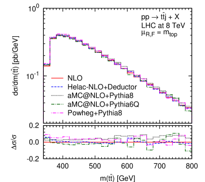
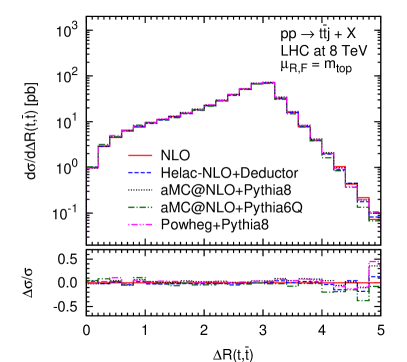
Refer to caption
Refer to caption
Figure 15: Differential cross section distributions as a function of the invariant mass of the tt¯𝑡¯𝑡t\bar{t} pair (left panel) and of the ΔRtt¯Δsubscript𝑅𝑡¯𝑡\Delta R_{t\bar{t}} (right panel) for pptt¯j+X𝑝𝑝𝑡¯𝑡𝑗𝑋pp\to t\bar{t}j+X at the LHC with s=8𝑠8\sqrt{s}=8 TeV. Comparison between the NLO result obtained with Helac-Nlo and results produced by matching various NLO predictions to different parton showers. The scale choice is μF=μR=mtsubscript𝜇𝐹subscript𝜇𝑅subscript𝑚𝑡\mu_{F}=\mu_{R}=m_{t}. The lower panels display the relative deviation from the fixed order result.
Refer to caption
Refer to caption
Figure 16: Differential cross section distributions as a function of the transverse momentum of the tt¯j1𝑡¯𝑡subscript𝑗1t\bar{t}j_{1} system for pptt¯j+X𝑝𝑝𝑡¯𝑡𝑗𝑋pp\to t\bar{t}j+X at the LHC with s=8𝑠8\sqrt{s}=8 TeV. Comparison between the NLO result obtained with Helac-Nlo and results produced by matching various NLO predictions to different parton showers. The scale choice is μF=μR=mtsubscript𝜇𝐹subscript𝜇𝑅subscript𝑚𝑡\mu_{F}=\mu_{R}=m_{t}. The lower panels display the relative deviation from the fixed order result.
Refer to caption
Refer to caption
Figure 17: Differential cross section distributions as a function of the the transverse momentum (left panel) and rapidity of the second jet (left panel) for pptt¯j+X𝑝𝑝𝑡¯𝑡𝑗𝑋pp\to t\bar{t}j+X at the LHC with s=8𝑠8\sqrt{s}=8 TeV. Comparison between the NLO result obtained with Helac-Nlo and results produced by matching various NLO predictions to different parton showers. The scale choice is μF=μR=mtsubscript𝜇𝐹subscript𝜇𝑅subscript𝑚𝑡\mu_{F}=\mu_{R}=m_{t}. The lower panels display the relative deviation from the fixed order result.
Refer to caption
Refer to caption
Figure 18: Differential cross section distribution as a function of the transverse momentum of the tt¯𝑡¯𝑡t\bar{t} pair (left panel) and inclusive jet cross sections (right panel) for pptt¯j+X𝑝𝑝𝑡¯𝑡𝑗𝑋pp\to t\bar{t}j+X at the LHC with s=8𝑠8\sqrt{s}=8 TeV. Comparison between the NLO result obtained with Helac-Nlo and results produced by matching various NLO predictions to different parton showers. The scale choice is μF=μR=mtsubscript𝜇𝐹subscript𝜇𝑅subscript𝑚𝑡\mu_{F}=\mu_{R}=m_{t}. The lower panels display the relative deviation from the fixed order result.

The same conclusions can be drawn from Fig. 15, where we show the invariant mass of the tt¯𝑡¯𝑡t\bar{t} pair and the angular separation in the rapidity-azimuthal angle plane between the top and the anti-top quark

ΔRij=(yiyj)2+(ϕiϕj)2.Δsubscript𝑅𝑖𝑗superscriptsubscript𝑦𝑖subscript𝑦𝑗2superscriptsubscriptitalic-ϕ𝑖subscriptitalic-ϕ𝑗2\Delta R_{ij}=\sqrt{(y_{i}-y_{j})^{2}+(\phi_{i}-\phi_{j})^{2}}\,. (145)

Overall, we observe that results obtained within the Helac-Nlo+Deductor framework are consistent with those of the other Monte-Carlo event generators used in this study. Let us emphasize, that not only various showers but also different matching schemes with distinct systematic uncertainties are examined here.

To assess potential differences among showers and matching procedures used in our analysis, we turn to observables, which are sensitive to the initial conditions of the parton evolution. As an example, we present in Fig. 16 the differential cross section distribution as a function of the transverse momentum of the tt¯j1𝑡¯𝑡subscript𝑗1t\bar{t}j_{1} system. For clarity we give both a linear-scale (left panel) and a log-scale (right panel) version of the plot. We observe that the matching with Pythia8 yields similar results for both Mc@Nlo and Powheg, i.e. the hardest spectra and a lack of agreement with the fixed order prediction in the region where hard, well separated partons are produced. We have found discrepances even up to 120%percent120120\%. This suggests, that for the process at hand, initial condition of the transverse-momentum ordered shower from Pythia8 should be adjusted to restrict further the shower phase space where emissions become hard. On the other hand, aMc@Nlo+Pythia6Q nicely reproduces the NLO differential cross section in the high pTsubscript𝑝𝑇p_{T} region. We also note that it produces a softer spectrum. As for the Helac-Nlo+Deductor case, as already explained, the parameter t0subscript𝑡0t_{0} was chosen to preserve the NLO shape in the tail of the pTsubscript𝑝𝑇p_{T} spectrum of the tt¯j1𝑡¯𝑡subscript𝑗1t\bar{t}j_{1} system.

In Fig. 17, the kinematics of the second jet is analysed. To be more precise, distributions in the transverse momentum and in rapidity are given. There is a good agreement between the spectra of aMc@Nlo+Pythia6Q and Helac-Nlo+Deductor, with a somewhat narrower rapidity spectrum in the case of Helac-Nlo+Deductor. For aMc@Nlo+Pythia8 and Powheg+Pythia8, a difference in normalization can be observed, but the differential K𝐾K-factor remains flat. This can be explained by larger emission rates that increase the amount of radiation.

In Fig. 18, the differential cross section as a function of the transverse momentum of the tt¯𝑡¯𝑡t\bar{t} pair is presented. We observe a good agreement among all programs for pT>50subscript𝑝𝑇50p_{T}>50 GeV i.e. above the analysis cut. Below this value the prediction is only leading order accurate and thus strongly depends on the initial shower conditions. Also shown in Fig. 18 are inclusive jet cross sections. In the first (second) bin the exclusive cross section is accurate at next-to-leading order (leading order). Starting from the third bin on, cross sections are only described with leading-logarithmic accuracy via the parton shower alone. Results for exclusive cross sections with Njets=1subscript𝑁jets1N_{\rm jets}=1 and Njets=2subscript𝑁jets2N_{\rm jets}=2 are in agreement with our observations for other observables. The picture is vastly different for all showers, however, when Njets3subscript𝑁jets3N_{\rm jets}\geq 3. In this case, the Powheg+Pythia8 framework (aMc@Nlo+Pythia6Q) produces the highest (lowest) number of hard jets.

Framework σ[1jet]superscript𝜎delimited-[]absent1jet\sigma^{[\geq 1~{}{\rm jet}]} σ[2jets]superscript𝜎delimited-[]absent2jets\sigma^{[\geq 2~{}{\rm jets}]} σ[3jets]superscript𝜎delimited-[]absent3jets\sigma^{[\geq 3~{}{\rm jets}]} σ[4jets]superscript𝜎delimited-[]absent4jets\sigma^{[\geq 4~{}{\rm jets}]} σ[5jets]superscript𝜎delimited-[]absent5jets\sigma^{[\geq 5~{}{\rm jets}]}
Helac-Nlo+Deductor 86110 17204 2780 362 38
aMc@Nlo+Pythia6Q 84850 15030 1230 106 7
aMc@Nlo+Pythia8 89556 21872 3377 372 32
Powheg+Pythia8 89121 23744 5458 992 129
Table 2: Cross sections (in fb) for the inclusive jet rates at the LHC with s=8𝑠8\sqrt{s}=8 TeV, according to the default settings of the various codes.
Framework σ[2]/σ[1]superscript𝜎delimited-[]absent2superscript𝜎delimited-[]absent1\sigma^{[\geq 2]}/\sigma^{[\geq 1]} σ[3]/σ[2]superscript𝜎delimited-[]absent3superscript𝜎delimited-[]absent2\sigma^{[\geq 3]}/\sigma^{[\geq 2]} σ[4]/σ[3]superscript𝜎delimited-[]absent4superscript𝜎delimited-[]absent3\sigma^{[\geq 4]}/\sigma^{[\geq 3]} σ[5]/σ[4]superscript𝜎delimited-[]absent5superscript𝜎delimited-[]absent4\sigma^{[\geq 5]}/\sigma^{[\geq 4]}
Helac-Nlo+Deductor 0.20 0.16 0.13 0.10
aMc@Nlo+Pythia6Q 0.18 0.08 0.09 0.07
aMc@Nlo+Pythia8 0.24 0.15 0.11 0.09
Powheg+Pythia8 0.27 0.23 0.18 0.13
Table 3: Cross section ratios for (n+1)/n𝑛1𝑛(n+1)/n inclusive jet rates at the LHC with s=8𝑠8\sqrt{s}=8 TeV, according to the default settings of the various codes.

Finally, cross sections (in fb) for inclusive σ(tt¯+njets)𝜎𝑡¯𝑡𝑛jets\sigma(t\bar{t}+n~{}{\rm jets}) rates are presented in Table 2. Table 3 contains cross section ratios, i.e. σ(tt¯+n+1jets)/σ(tt¯+njets)𝜎𝑡¯𝑡𝑛1jets𝜎𝑡¯𝑡𝑛jets\sigma(t\bar{t}+n+1~{}{\rm jets})/\sigma(t\bar{t}+n~{}{\rm jets}).

6 Conclusions

In this publication, we have presented a next-to-leading order matching scheme for the Nagy-Soper parton shower. We based our construction on the original Mc@Nlo approach. Besides the general formulation, we have performed real simulations for top-quark pair production in association with a jet at the LHC, using an implementation within the framework of the public codes Helac-Nlo and Deductor.

Our general conclusion is that the combination Helac-Nlo+Deductor is able to provide results for non-trivial processes, which remain in reasonable agreement with other Monte Carlo systems. Indeed, for observables, which are rather insensitive to showering effects, the differential cross sections are in very good agreement between different programs and the fixed order NLO calculation. Inevitable differences for infrared sensitive observables, on the other hand, seem to be justifiable in size in the sense that all predictions have overlapping uncertainty bands. Of course, further studies are needed here.

We note that our simulations are at the same level of logarithmic precision as those of others. For now, we are only correct as far as the leading behaviour is concerned. Future developments in Deductor will allow us to include soft-gluon intereference effects yielding next-to-leading logarithmic accuracy. This step still requires some improvements of our implementation in Helac-Dipoles. In particular, it will be necessary to transfer colour-configuration information exactly, as opposed to the current leading-colour approximation. We leave this to future work.

Finally, we expect that the Nagy-Soper parton shower will open new opportunities for understanding parton shower systematics for processes with non-trivial colour exchange. Here, the road is still long, as we must remember that, ultimately, hadronization models must be included. The latter, however, require tuning to the shower. There are also interesting problems in merging different multiplicity samples generated by our software.

Acknowledgements

We would like to thank M. Krämer and Z. Nagy for discussions at preliminary stages of this study. The work of M. Czakon and H. Hartanto was supported by the German Research Foundation (DFG) via the Sonderforschungsbereich/Transregio SFB/TR-9 “Computational Particle Physics”. M. Worek and M. Kraus acknowledge support by the DFG under Grant No. WO 1900/1-1 (“Signals and Backgrounds Beyond Leading Order. Phenomenological studies for the LHC ”). In addition, this research was supported in part by the Research Funding Program ARISTEIA, HOCTools (co-financed by the European Union (European Social Fund ESF) and Greek national funds through the Operational Program "Education and Lifelong Learning" of the National Strategic Reference Framework (NSRF)).

Appendix A Simplified matching scheme

In this Appendix, we discuss the simplified matching prescription that we have implemented starting from spin and colour averaged amplitudes. We also prove that it yields NLO accuracy at leading colour, as long as the observable is not sensitive to spin correlations. The simplifications match the current Deductor functionality and relate to a spin and colour averaged quantum density

|ρ)=m1m![d{p,f}m]|{p,f}m)({p,f}m|ρ),|\rho)=\sum_{m}\frac{1}{m!}\int[d\{p,f\}_{m}]|\{p,f\}_{m})(\{p,f\}_{m}|\rho)\;, (146)

where

({p,f}m|ρ)={s}m,{s}m{c}m,{c}m{s,c}m|{s,c}mρ({p,f,s,c,s,c}m).conditionalsubscript𝑝𝑓𝑚𝜌subscriptsubscript𝑠𝑚subscriptsuperscript𝑠𝑚subscriptsubscript𝑐𝑚subscriptsuperscript𝑐𝑚inner-productsubscript𝑠𝑐𝑚subscriptsuperscript𝑠superscript𝑐𝑚𝜌subscript𝑝𝑓superscript𝑠superscript𝑐𝑠𝑐𝑚(\{p,f\}_{m}|\rho)=\sum_{\{s\}_{m},\{s^{\prime}\}_{m}}\sum_{\{c\}_{m},\{c^{\prime}\}_{m}}\braket{\{s,c\}_{m}}{\{s^{\prime},c^{\prime}\}_{m}}\rho(\{p,f,s^{\prime},c^{\prime},s,c\}_{m})\;. (147)

Averaging over spin and colour reduces tremendously the complexity of the calculation. However, the parton shower requires a colour configuration for each phase space point {p,f}msubscript𝑝𝑓𝑚\{p,f\}_{m} in order to perform the evolution. Starting from colour averaged weights ({p,f}m|ρ)conditionalsubscript𝑝𝑓𝑚𝜌(\{p,f\}_{m}|\rho) one can recover leading colour correlations, ({p,f,c}m|ρ)conditionalsubscript𝑝𝑓𝑐𝑚𝜌(\{p,f,c\}_{m}|\rho), by including a colour weight Cw({p,f,c}m)subscript𝐶𝑤subscript𝑝𝑓𝑐𝑚C_{w}(\{p,f,c\}_{m}), defined by

Cw({p,f,c}m)=({p,f,c}m|ρm(0)){c^}m({p,f,c^}m|ρm(0)).subscript𝐶𝑤subscript𝑝𝑓𝑐𝑚conditionalsubscript𝑝𝑓𝑐𝑚subscriptsuperscript𝜌0𝑚subscriptsubscript^𝑐𝑚conditionalsubscript𝑝𝑓^𝑐𝑚subscriptsuperscript𝜌0𝑚C_{w}(\{p,f,c\}_{m})=\frac{(\{p,f,c\}_{m}|\rho^{(0)}_{m})}{\sum_{\{\hat{c}\}_{m}}(\{p,f,\hat{c}\}_{m}|\rho^{(0)}_{m})}\;. (148)

The simplified matching prescription accounting for generation cuts is then

σ[F]=[d{p,f,c}m]m!(F|U(tF,t0)|{p,f,c}m)Cw({p,f,c}m)({p,f}m|Ω|ρm(0))FI({p,f}m)+[d{p,f,c}m+1](m+1)!(F|U(tF,t0)|{p,f,c}m+1)Cw({p,f,c}m+1)×({p,f}m+1|R)FI({p,f}m+1)σm[F]+σm+1[F],𝜎delimited-[]𝐹delimited-[]𝑑subscript𝑝𝑓𝑐𝑚𝑚𝐹𝑈subscript𝑡𝐹subscript𝑡0subscript𝑝𝑓𝑐𝑚subscript𝐶𝑤subscript𝑝𝑓𝑐𝑚subscript𝑝𝑓𝑚Ωsubscriptsuperscript𝜌0𝑚subscript𝐹𝐼subscript𝑝𝑓𝑚delimited-[]𝑑subscript𝑝𝑓𝑐𝑚1𝑚1𝐹𝑈subscript𝑡𝐹subscript𝑡0subscript𝑝𝑓𝑐𝑚1subscript𝐶𝑤subscript𝑝𝑓𝑐𝑚1conditionalsubscript𝑝𝑓𝑚1𝑅subscript𝐹𝐼subscript𝑝𝑓𝑚1subscript𝜎𝑚delimited-[]𝐹subscript𝜎𝑚1delimited-[]𝐹\begin{split}\sigma[F]&=\int\frac{[d\{p,f,c\}_{m}]}{m!}(F|U(t_{F},t_{0})|\{p,f,c\}_{m})C_{w}(\{p,f,c\}_{m})(\{p,f\}_{m}|\Omega|\rho^{(0)}_{m})F_{I}(\{p,f\}_{m})\\ &+\int\frac{[d\{p,f,c\}_{m+1}]}{(m+1)!}(F|U(t_{F},t_{0})|\{p,f,c\}_{m+1})C_{w}(\{p,f,c\}_{m+1})\\ &\quad\times(\{p,f\}_{m+1}|R)F_{I}(\{p,f\}_{m+1})\\[5.69046pt] &\equiv\sigma_{m}[F]+\sigma_{m+1}[F]\;,\end{split} (149)

where the action of the operator ΩΩ\Omega is given by

({p,f}m|Ω|ρm(0))=ω({p,f}m)({p,f}m|ρm(0)),subscript𝑝𝑓𝑚Ωsubscriptsuperscript𝜌0𝑚𝜔subscript𝑝𝑓𝑚conditionalsubscript𝑝𝑓𝑚subscriptsuperscript𝜌0𝑚(\{p,f\}_{m}|\Omega|\rho^{(0)}_{m})=\omega(\{p,f\}_{m})(\{p,f\}_{m}|\rho^{(0)}_{m})\;, (150)

with

ω({p,f}m)=1+({p,f}m|ρm(1))({p,f}m|ρm(0))+({p,f}m|𝐈(t0)+𝐊(t0)+𝐏|ρm(0))({p,f}m|ρm(0)).𝜔subscript𝑝𝑓𝑚1conditionalsubscript𝑝𝑓𝑚subscriptsuperscript𝜌1𝑚conditionalsubscript𝑝𝑓𝑚subscriptsuperscript𝜌0𝑚subscript𝑝𝑓𝑚𝐈subscript𝑡0𝐊subscript𝑡0𝐏subscriptsuperscript𝜌0𝑚conditionalsubscript𝑝𝑓𝑚subscriptsuperscript𝜌0𝑚\omega(\{p,f\}_{m})=1+\frac{(\{p,f\}_{m}|\rho^{(1)}_{m})}{(\{p,f\}_{m}|\rho^{(0)}_{m})}+\frac{(\{p,f\}_{m}|\mathbf{I}(t_{0})+\mathbf{K}(t_{0})+\mathbf{P}|\rho^{(0)}_{m})}{(\{p,f\}_{m}|\rho^{(0)}_{m})}\;. (151)

The density matrix for the real subtracted cross section, ({p,f}m+1|R)conditionalsubscript𝑝𝑓𝑚1𝑅(\{p,f\}_{m+1}|R), is defined as

({p,f}m+1|R)({p,f}m+1|ρm+1(0))t0𝑑τ{s,s,c,c}{s,c}m+1|{s,c}m+1×[d{p^,f^,s^,c^,s^,c^}m]m!({p^,f^,s^,c^,s^,c^}m|ρm(0))FI({p^,f^}m)×({p,f,s,c,s,c}m+1|I(τ)|{p^,f^,s^,c^,s^,c^}m),conditionalsubscript𝑝𝑓𝑚1𝑅conditionalsubscript𝑝𝑓𝑚1subscriptsuperscript𝜌0𝑚1superscriptsubscriptsubscript𝑡0differential-d𝜏subscript𝑠superscript𝑠𝑐superscript𝑐inner-productsubscriptsuperscript𝑠superscript𝑐𝑚1subscript𝑠𝑐𝑚1delimited-[]𝑑subscript^𝑝^𝑓superscript^𝑠superscript^𝑐^𝑠^𝑐𝑚𝑚|subscript^𝑝^𝑓superscript^𝑠superscript^𝑐^𝑠^𝑐𝑚subscriptsuperscript𝜌0𝑚subscript𝐹𝐼subscript^𝑝^𝑓𝑚subscript𝑝𝑓superscript𝑠superscript𝑐𝑠𝑐𝑚1subscript𝐼𝜏subscript^𝑝^𝑓superscript^𝑠superscript^𝑐^𝑠^𝑐𝑚\begin{split}(\{p,f\}_{m+1}|R)&\equiv(\{p,f\}_{m+1}|\rho^{(0)}_{m+1})-\int_{t_{0}}^{\infty}d\tau~{}\sum_{\{s,s^{\prime},c,c^{\prime}\}}\braket{\{s^{\prime},c^{\prime}\}_{m+1}}{\{s,c\}_{m+1}}\\ &\times\int\frac{[d\{\hat{p},\hat{f},\hat{s}^{\prime},\hat{c}^{\prime},\hat{s},\hat{c}\}_{m}]}{m!}(\{\hat{p},\hat{f},\hat{s}^{\prime},\hat{c}^{\prime},\hat{s},\hat{c}\}_{m}|\rho^{(0)}_{m})\;F_{I}(\{\hat{p},\hat{f}\}_{m})\\[5.69046pt] &\times(\{p,f,s^{\prime},c^{\prime},s,c\}_{m+1}|\mathcal{H}_{I}(\tau)|\{\hat{p},\hat{f},\hat{s}^{\prime},\hat{c}^{\prime},\hat{s},\hat{c}\}_{m})\;,\end{split} (152)

where we specified explicitly the full quantum correlations in the subtraction terms required for the removal of kinematic singularities. I(t)subscript𝐼𝑡\mathcal{H}_{I}(t) is the Nagy-Soper real splitting operator without any approximations. The inclusive jet functions FI({p,f}m)subscript𝐹𝐼subscript𝑝𝑓𝑚F_{I}(\{p,f\}_{m}) define the generation cuts.

Let us now study the accuracy of Eq. (149) after expansion to next-to-leading order. The parton shower evolution operator, currently available in Deductor, reads

U(tF,t0)=NLC+(tF,t0)+t0tF𝑑τU(tF,τ)¯ILC+(τ)NLC+(τ,t0),𝑈subscript𝑡𝐹subscript𝑡0superscript𝑁limit-from𝐿𝐶subscript𝑡𝐹subscript𝑡0superscriptsubscriptsubscript𝑡0subscript𝑡𝐹differential-d𝜏𝑈subscript𝑡𝐹𝜏superscriptsubscript¯𝐼limit-from𝐿𝐶𝜏superscript𝑁limit-from𝐿𝐶𝜏subscript𝑡0U(t_{F},t_{0})=N^{LC+}(t_{F},t_{0})+\int_{t_{0}}^{t_{F}}d\tau~{}U(t_{F},\tau)\overline{\mathcal{H}}_{I}^{LC+}(\tau)N^{LC+}(\tau,t_{0})\;, (153)

where ¯ILC+(τ)superscriptsubscript¯𝐼limit-from𝐿𝐶𝜏\overline{\mathcal{H}}_{I}^{LC+}(\tau) denotes the spin averaged splitting operator in the LC+ approximation and NLC+(tF,t0)superscript𝑁limit-from𝐿𝐶subscript𝑡𝐹subscript𝑡0N^{LC+}(t_{F},t_{0}) the corresponding Sudakov form factor, as discussed in Section 2.6. Inserting Eq. (153) in σm[F]subscript𝜎𝑚delimited-[]𝐹\sigma_{m}[F] and expanding the evolution yields

σm[F]=1m![d{p,f,c}m](F|{p,f,c}m)Cw({p,f,c}m)({p,f}m|Ω|ρm(0))FI({p,f}m)+1m![d{p,f,c}m]t0tF𝑑τ(F|¯ILC+(τ)𝒱LC+(τ)|{p,f,c}m)×Cw({p,f,c}m)({p,f}m|ρm(0))FI({p,f}m)+𝒪(αs2).subscript𝜎𝑚delimited-[]𝐹1𝑚delimited-[]𝑑subscript𝑝𝑓𝑐𝑚conditional𝐹subscript𝑝𝑓𝑐𝑚subscript𝐶𝑤subscript𝑝𝑓𝑐𝑚subscript𝑝𝑓𝑚Ωsubscriptsuperscript𝜌0𝑚subscript𝐹𝐼subscript𝑝𝑓𝑚1𝑚delimited-[]𝑑subscript𝑝𝑓𝑐𝑚superscriptsubscriptsubscript𝑡0subscript𝑡𝐹differential-d𝜏𝐹superscriptsubscript¯𝐼limit-from𝐿𝐶𝜏superscript𝒱limit-from𝐿𝐶𝜏subscript𝑝𝑓𝑐𝑚subscript𝐶𝑤subscript𝑝𝑓𝑐𝑚conditionalsubscript𝑝𝑓𝑚subscriptsuperscript𝜌0𝑚subscript𝐹𝐼subscript𝑝𝑓𝑚𝒪superscriptsubscript𝛼𝑠2\begin{split}\sigma_{m}[F]&=\frac{1}{m!}\int[d\{p,f,c\}_{m}](F|\{p,f,c\}_{m})C_{w}(\{p,f,c\}_{m})(\{p,f\}_{m}|\Omega|\rho^{(0)}_{m})F_{I}(\{p,f\}_{m})\\ &+\frac{1}{m!}\int[d\{p,f,c\}_{m}]\int_{t_{0}}^{t_{F}}d\tau~{}(F|\overline{\mathcal{H}}_{I}^{LC+}(\tau)-\mathcal{V}^{LC+}(\tau)|\{p,f,c\}_{m})\\[5.69046pt] &\times C_{w}(\{p,f,c\}_{m})(\{p,f\}_{m}|\rho^{(0)}_{m})F_{I}(\{p,f\}_{m})+\mathcal{O}(\alpha_{s}^{2})\;.\end{split} (154)

Using the approximations

𝒱(τ)=𝒱LC+(τ)+𝒪(1/Nc2),𝒱𝜏superscript𝒱limit-from𝐿𝐶𝜏𝒪1superscriptsubscript𝑁𝑐2\mathcal{V}(\tau)=\mathcal{V}^{LC+}(\tau)+\mathcal{O}(1/N_{c}^{2})\;, (155)

and

Cw({p,f,c}m)({p,f}m|ρm(0,1))=({p,f,c}m|ρm(0,1))+𝒪(1/Nc2),subscript𝐶𝑤subscript𝑝𝑓𝑐𝑚conditionalsubscript𝑝𝑓𝑚subscriptsuperscript𝜌01𝑚conditionalsubscript𝑝𝑓𝑐𝑚subscriptsuperscript𝜌01𝑚𝒪1superscriptsubscript𝑁𝑐2C_{w}(\{p,f,c\}_{m})(\{p,f\}_{m}|\rho^{(0,1)}_{m})=(\{p,f,c\}_{m}|\rho^{(0,1)}_{m})+\mathcal{O}(1/N_{c}^{2})\;, (156)

Eq. (154) reduces to

σm[F]=1m![d{p,f,c}m](F|{p,f,c}m)({p,f,c}m|[|ρm(0))+|ρm(1))+𝐏|ρm(0))]FI({p,f}m)+1m![d{p,f,c}m]t0𝑑τ(F|¯ILC+(τ)|{p,f,c}m)({p,f,c}m|ρm(0))FI({p,f}m)+𝒪(αs2,1/Nc2,Δσ).\begin{split}\sigma_{m}[F]&=\frac{1}{m!}\int[d\{p,f,c\}_{m}](F|\{p,f,c\}_{m})(\{p,f,c\}_{m}|\left[|\rho^{(0)}_{m})+|\rho^{(1)}_{m})+\mathbf{P}|\rho^{(0)}_{m})\right]F_{I}(\{p,f\}_{m})\\ &+\frac{1}{m!}\int[d\{p,f,c\}_{m}]\int_{t_{0}}^{\infty}d\tau~{}(F|\overline{\mathcal{H}}_{I}^{LC+}(\tau)|\{p,f,c\}_{m})(\{p,f,c\}_{m}|\rho^{(0)}_{m})F_{I}(\{p,f\}_{m})\\ &+\mathcal{O}(\alpha_{s}^{2},1/N_{c}^{2},\Delta\sigma)\;.\end{split} (157)

Here, ΔσΔ𝜎\Delta\sigma represents the error resulting from the limit tFsubscript𝑡𝐹t_{F}\to\infty.

Let us now turn to the σm+1[F]subscript𝜎𝑚1delimited-[]𝐹\sigma_{m+1}[F]. Expanding the shower evolution and making use of Eq. (156) to recover the leading colour correlated real matrix element, we find

σm+1[F]=[d{p,f,c}m+1](m+1)!(F|{p,f,c}m+1)FI({p,f}m+1)[({p,f,c}m+1|ρm+1(0))t0𝑑τ{s¯,s¯,c¯,c¯}m+1{s¯,c¯}m+1|{s¯,c¯}m+1Cw({p,f,c}m+1)×[d{p^,f^,s^,c^,s^,c^}m]m!({p^,f^,s^,c^,s^,c^}m|ρm(0))FI({p^,f^}m)×({p,f,s¯,c¯,s¯,c¯}m+1|I(τ)|{p^,f^,s^,c^,s^,c^}m)]+𝒪(αs2,1/Nc2)σm+1R[F]σm+1S[F]+𝒪(αs2,1/Nc2).\begin{split}\sigma_{m+1}[F]&=\int\frac{[d\{p,f,c\}_{m+1}]}{(m+1)!}(F|\{p,f,c\}_{m+1})F_{I}(\{p,f\}_{m+1})\Biggl{[}(\{p,f,c\}_{m+1}|\rho^{(0)}_{m+1})\\ &-\int_{t_{0}}^{\infty}d\tau\sum_{\{\bar{s},\bar{s}^{\prime},\bar{c}^{\prime},\bar{c}\}_{m+1}}\braket{\{\bar{s}^{\prime},\bar{c}^{\prime}\}_{m+1}}{\{\bar{s},\bar{c}\}_{m+1}}C_{w}(\{p,f,c\}_{m+1})\\ &\times\int\frac{[d\{\hat{p},\hat{f},\hat{s}^{\prime},\hat{c}^{\prime},\hat{s},\hat{c}\}_{m}]}{m!}(\{\hat{p},\hat{f},\hat{s}^{\prime},\hat{c}^{\prime},\hat{s},\hat{c}\}_{m}|\rho^{(0)}_{m})\;F_{I}(\{\hat{p},\hat{f}\}_{m})\\ &\times(\{p,f,\bar{s}^{\prime},\bar{c}^{\prime},\bar{s},\bar{c}\}_{m+1}|\mathcal{H}_{I}(\tau)|\{\hat{p},\hat{f},\hat{s}^{\prime},\hat{c}^{\prime},\hat{s},\hat{c}\}_{m})\Biggl{]}+\mathcal{O}(\alpha_{s}^{2},1/N_{c}^{2})\\ &\equiv\sigma^{R}_{m+1}[F]-\sigma^{S}_{m+1}[F]+\mathcal{O}(\alpha_{s}^{2},1/N_{c}^{2})\;.\end{split} (158)

In the following we will focus on the subtraction terms σm+1S[F]subscriptsuperscript𝜎𝑆𝑚1delimited-[]𝐹\sigma^{S}_{m+1}[F]. The summation over {c}m+1subscript𝑐𝑚1\{c\}_{m+1} can be eliminated by

[d{p,f,c}m+1]Cw({p,f,c}m+1)(F|{p,f,c}m+1)=[d{p,f}m+1](F|{p,f}m+1)+𝒪(1/Nc2).delimited-[]𝑑subscript𝑝𝑓𝑐𝑚1subscript𝐶𝑤subscript𝑝𝑓𝑐𝑚1conditional𝐹subscript𝑝𝑓𝑐𝑚1delimited-[]𝑑subscript𝑝𝑓𝑚1conditional𝐹subscript𝑝𝑓𝑚1𝒪1superscriptsubscript𝑁𝑐2\begin{split}\int[d\{p,f,c\}_{m+1}]&C_{w}(\{p,f,c\}_{m+1})(F|\{p,f,c\}_{m+1})\\ &=\int[d\{p,f\}_{m+1}](F|\{p,f\}_{m+1})+\mathcal{O}(1/N_{c}^{2})\;.\end{split} (159)

By a further approximation to the colour correlator

{c¯}m+1|{c¯}m+1={c¯}m+1|{c¯}m+1δ({c¯}m+1;{c¯}m+1)+𝒪(1/Nc2),inner-productsubscriptsuperscript¯𝑐𝑚1subscript¯𝑐𝑚1inner-productsubscript¯𝑐𝑚1subscript¯𝑐𝑚1𝛿subscriptsuperscript¯𝑐𝑚1subscript¯𝑐𝑚1𝒪1superscriptsubscript𝑁𝑐2\begin{split}\braket{\{\bar{c}^{\prime}\}_{m+1}}{\{\bar{c}\}_{m+1}}&=\braket{\{\bar{c}\}_{m+1}}{\{\bar{c}\}_{m+1}}\delta\left(\{\bar{c}^{\prime}\}_{m+1};\{\bar{c}\}_{m+1}\right)+\mathcal{O}(1/N_{c}^{2})\;,\end{split} (160)

we recover leading colour correlations

[d{p,f}m+1]{c¯}m+1(F|{p,f}m+1){c¯}m+1|{c¯}m+1=[d{p,f,c¯}m+1](F|{p,f,c¯}m+1).delimited-[]𝑑subscript𝑝𝑓𝑚1subscriptsubscript¯𝑐𝑚1conditional𝐹subscript𝑝𝑓𝑚1inner-productsubscript¯𝑐𝑚1subscript¯𝑐𝑚1delimited-[]𝑑subscript𝑝𝑓¯𝑐𝑚1conditional𝐹subscript𝑝𝑓¯𝑐𝑚1\begin{split}\int[d\{p,f\}_{m+1}]\sum_{\{\bar{c}\}_{m+1}}(F|\{p,f\}_{m+1})&\braket{\{\bar{c}\}_{m+1}}{\{\bar{c}\}_{m+1}}\\ &=\int[d\{p,f,\bar{c}\}_{m+1}](F|\{p,f,\bar{c}\}_{m+1})\;.\end{split} (161)

In the following we rename c¯c¯𝑐𝑐\bar{c}\to c and drop the second colour index in ({p,f,s¯,c,s¯,c}m+1|(\{p,f,\bar{s}^{\prime},c,\bar{s},c\}_{m+1}|. In addition, we use

I(τ)=ILC+(τ)+𝒪(1/Nc2),subscript𝐼𝜏superscriptsubscript𝐼limit-from𝐿𝐶𝜏𝒪1superscriptsubscript𝑁𝑐2\mathcal{H}_{I}(\tau)=\mathcal{H}_{I}^{LC+}(\tau)+\mathcal{O}(1/N_{c}^{2})\;, (162)

to obtain the following form for σm+1S[F]superscriptsubscript𝜎𝑚1𝑆delimited-[]𝐹\sigma_{m+1}^{S}[F]

σm+1S[F]=1(m+1)!m![d{p,f,c}m+1][d{p^,f^,s^,c^,s^,c^}m]FI({p^,f^}m)FI({p,f}m+1)×(F|{p,f,c}m+1)t0𝑑τ{s¯,s¯}m+1{s¯}m+1|{s¯}m+1({p^,f^,s^,c^,s^,c^}m|ρm(0))×({p,f,s¯,s¯,c}m+1|ILC+(τ)|{p^,f^,s^,c^,s^,c^}m)+𝒪(αs2,1/Nc2).superscriptsubscript𝜎𝑚1𝑆delimited-[]𝐹1𝑚1𝑚delimited-[]𝑑subscript𝑝𝑓𝑐𝑚1delimited-[]𝑑subscript^𝑝^𝑓superscript^𝑠superscript^𝑐^𝑠^𝑐𝑚subscript𝐹𝐼subscript^𝑝^𝑓𝑚subscript𝐹𝐼subscript𝑝𝑓𝑚1conditional𝐹subscript𝑝𝑓𝑐𝑚1superscriptsubscriptsubscript𝑡0differential-d𝜏subscriptsubscript¯𝑠superscript¯𝑠𝑚1inner-productsubscriptsuperscript¯𝑠𝑚1subscript¯𝑠𝑚1conditionalsubscript^𝑝^𝑓superscript^𝑠superscript^𝑐^𝑠^𝑐𝑚subscriptsuperscript𝜌0𝑚subscript𝑝𝑓superscript¯𝑠¯𝑠𝑐𝑚1subscriptsuperscriptlimit-from𝐿𝐶𝐼𝜏subscript^𝑝^𝑓superscript^𝑠superscript^𝑐^𝑠^𝑐𝑚𝒪superscriptsubscript𝛼𝑠21superscriptsubscript𝑁𝑐2\begin{split}\sigma_{m+1}^{S}[F]&=\frac{1}{(m+1)!m!}\int[d\{p,f,c\}_{m+1}][d\{\hat{p},\hat{f},\hat{s}^{\prime},\hat{c}^{\prime},\hat{s},\hat{c}\}_{m}]F_{I}(\{\hat{p},\hat{f}\}_{m})F_{I}(\{p,f\}_{m+1})\\ &\times(F|\{p,f,c\}_{m+1})\int_{t_{0}}^{\infty}d\tau\sum_{\{\bar{s},\bar{s}^{\prime}\}_{m+1}}\braket{\{\bar{s}^{\prime}\}_{m+1}}{\{\bar{s}\}_{m+1}}(\{\hat{p},\hat{f},\hat{s}^{\prime},\hat{c}^{\prime},\hat{s},\hat{c}\}_{m}|\rho^{(0)}_{m})\\ &\times(\{p,f,\bar{s}^{\prime},\bar{s},c\}_{m+1}|\mathcal{H}^{LC+}_{I}(\tau)|\{\hat{p},\hat{f},\hat{s}^{\prime},\hat{c}^{\prime},\hat{s},\hat{c}\}_{m})+\mathcal{O}(\alpha_{s}^{2},1/N_{c}^{2})\;.\end{split} (163)

It is now necessary to remove spin correlations. This can only be achieved, if (F|{p,f,c}m+1)conditional𝐹subscript𝑝𝑓𝑐𝑚1(F|\{p,f,c\}_{m+1}) and FI({p,f}m+1)subscript𝐹𝐼subscript𝑝𝑓𝑚1F_{I}(\{p,f\}_{m+1}) are sufficiently inclusive to allow an azimuthal average. A typical case would be an observable with NLO accuracy, where the azimuthal average corresponds to the complete phase space integral over unresolved jets. On the example of top-quark pair production with at least one jet, this would be any observable insensitive to additional jets. Once an azimuthal average has been performed, spin correlations vanish as demonstrated in Ref. Nagy:2007ty (Chapter 12)

dϕ2π{s¯,s¯}m+1{s¯}m+1|{s¯}m+1({p,f,s¯,s¯,c}m+1|ILC+(τ)|{p^,f^,s^,c^,s^,c^}m)={s^}m|{s^}m({p,f,c}m+1|¯ILC+(τ)|{p^,f^,c^,c^}m),𝑑italic-ϕ2𝜋subscriptsubscript¯𝑠superscript¯𝑠𝑚1inner-productsubscriptsuperscript¯𝑠𝑚1subscript¯𝑠𝑚1subscript𝑝𝑓superscript¯𝑠¯𝑠𝑐𝑚1subscriptsuperscriptlimit-from𝐿𝐶𝐼𝜏subscript^𝑝^𝑓superscript^𝑠superscript^𝑐^𝑠^𝑐𝑚inner-productsubscriptsuperscript^𝑠𝑚subscript^𝑠𝑚subscript𝑝𝑓𝑐𝑚1subscriptsuperscript¯limit-from𝐿𝐶𝐼𝜏subscript^𝑝^𝑓superscript^𝑐^𝑐𝑚\begin{split}\int\frac{d\phi}{2\pi}&\sum_{\{\bar{s},\bar{s}^{\prime}\}_{m+1}}\braket{\{\bar{s}^{\prime}\}_{m+1}}{\{\bar{s}\}_{m+1}}(\{p,f,\bar{s}^{\prime},\bar{s},c\}_{m+1}|\mathcal{H}^{LC+}_{I}(\tau)|\{\hat{p},\hat{f},\hat{s}^{\prime},\hat{c}^{\prime},\hat{s},\hat{c}\}_{m})\\ &=\braket{\{\hat{s}^{\prime}\}_{m}}{\{\hat{s}\}_{m}}(\{p,f,c\}_{m+1}|\overline{\mathcal{H}}^{LC+}_{I}(\tau)|\{\hat{p},\hat{f},\hat{c}^{\prime},\hat{c}\}_{m})\;,\end{split} (164)

which can be further transformed with

({p,f,c}m+1|¯ILC+(τ)|{p^,f^,c^,c^}m)=({p,f,c}m+1|¯ILC+(τ)|{p^,f^,c^}m)×δ({c^}m;{c^}m)+𝒪(1/Nc2).subscript𝑝𝑓𝑐𝑚1subscriptsuperscript¯limit-from𝐿𝐶𝐼𝜏subscript^𝑝^𝑓superscript^𝑐^𝑐𝑚subscript𝑝𝑓𝑐𝑚1subscriptsuperscript¯limit-from𝐿𝐶𝐼𝜏subscript^𝑝^𝑓^𝑐𝑚𝛿subscriptsuperscript^𝑐𝑚subscript^𝑐𝑚𝒪1superscriptsubscript𝑁𝑐2\begin{split}(\{p,f,c\}_{m+1}|\overline{\mathcal{H}}^{LC+}_{I}(\tau)|\{\hat{p},\hat{f},\hat{c}^{\prime},\hat{c}\}_{m})&=(\{p,f,c\}_{m+1}|\overline{\mathcal{H}}^{LC+}_{I}(\tau)|\{\hat{p},\hat{f},\hat{c}\}_{m})\\ &\times\delta\left(\{\hat{c}^{\prime}\}_{m};\{\hat{c}\}_{m}\right)+\mathcal{O}(1/N_{c}^{2})\;.\end{split} (165)

Substituting Eq. (164) and Eq. (165) into Eq. (163) we obtain

σm+1S[F]=1(m+1)!m![d{p,f,c}m+1][d{p^,f^,c^}m](F|{p,f,c}m+1)×t0dτ({p,f,c}m+1|¯ILC+(τ)|{p^,f^,c^}m)FI({p^,f^}m)FI({p,f}m+1)×{s^,s^}m{s^}m|{s^}m({p^,f^,s^,s^,c^}m|ρm(0))+𝒪(αs2,1/Nc2).superscriptsubscript𝜎𝑚1𝑆delimited-[]𝐹1𝑚1𝑚delimited-[]𝑑subscript𝑝𝑓𝑐𝑚1delimited-[]𝑑subscript^𝑝^𝑓^𝑐𝑚conditional𝐹subscript𝑝𝑓𝑐𝑚1superscriptsubscriptsubscript𝑡0𝑑𝜏subscript𝑝𝑓𝑐𝑚1subscriptsuperscript¯limit-from𝐿𝐶𝐼𝜏subscript^𝑝^𝑓^𝑐𝑚subscript𝐹𝐼subscript^𝑝^𝑓𝑚subscript𝐹𝐼subscript𝑝𝑓𝑚1subscriptsubscript^𝑠superscript^𝑠𝑚inner-productsubscriptsuperscript^𝑠𝑚subscript^𝑠𝑚|subscript^𝑝^𝑓superscript^𝑠^𝑠^𝑐𝑚subscriptsuperscript𝜌0𝑚𝒪superscriptsubscript𝛼𝑠21superscriptsubscript𝑁𝑐2\begin{split}\sigma_{m+1}^{S}[F]&=\frac{1}{(m+1)!m!}\int[d\{p,f,c\}_{m+1}][d\{\hat{p},\hat{f},\hat{c}\}_{m}](F|\{p,f,c\}_{m+1})\\ &\times\int_{t_{0}}^{\infty}d\tau(\{p,f,c\}_{m+1}|\overline{\mathcal{H}}^{LC+}_{I}(\tau)|\{\hat{p},\hat{f},\hat{c}\}_{m})F_{I}(\{\hat{p},\hat{f}\}_{m})F_{I}(\{p,f\}_{m+1})\\ &\times\sum_{\{\hat{s},\hat{s}^{\prime}\}_{m}}\braket{\{\hat{s}^{\prime}\}_{m}}{\{\hat{s}\}_{m}}(\{\hat{p},\hat{f},\hat{s}^{\prime},\hat{s},\hat{c}\}_{m}|\rho^{(0)}_{m})+\mathcal{O}(\alpha_{s}^{2},1/N_{c}^{2})\;.\end{split} (166)

The last line of Eq. (166) corresponds to the leading colour, spin averaged quantum density matrix

{s^,s^}m{s^}m|{s^}m({p^,f^,s^,s^,c^}m|ρm(0))=({p^,f^,c^}m|ρm(0)).subscriptsubscript^𝑠superscript^𝑠𝑚inner-productsubscriptsuperscript^𝑠𝑚subscript^𝑠𝑚conditionalsubscript^𝑝^𝑓superscript^𝑠^𝑠^𝑐𝑚subscriptsuperscript𝜌0𝑚conditionalsubscript^𝑝^𝑓^𝑐𝑚subscriptsuperscript𝜌0𝑚\sum_{\{\hat{s},\hat{s}^{\prime}\}_{m}}\braket{\{\hat{s}^{\prime}\}_{m}}{\{\hat{s}\}_{m}}(\{\hat{p},\hat{f},\hat{s}^{\prime},\hat{s},\hat{c}\}_{m}|\rho^{(0)}_{m})=(\{\hat{p},\hat{f},\hat{c}\}_{m}|\rho^{(0)}_{m})\;. (167)

With these approximations the final expression for σm+1S[F]subscriptsuperscript𝜎𝑆𝑚1delimited-[]𝐹\sigma^{S}_{m+1}[F] reads

σm+1S[F]=1(m+1)!m![d{p^,f^,c^}m+1][d{p,f,c}m]t0tF𝑑τ(F|{p^,f^,c^}m+1)×FI({p^,f^}m+1)({p^,f^,c^}m+1|¯ILC+(τ)|{p,f,c}m)×({p,f,c}m|ρm(0))FI({p,f}m)+𝒪(αs2,1/Nc2,Δσ).subscriptsuperscript𝜎𝑆𝑚1delimited-[]𝐹1𝑚1𝑚delimited-[]𝑑subscript^𝑝^𝑓^𝑐𝑚1delimited-[]𝑑subscript𝑝𝑓𝑐𝑚superscriptsubscriptsubscript𝑡0subscript𝑡𝐹differential-d𝜏conditional𝐹subscript^𝑝^𝑓^𝑐𝑚1subscript𝐹𝐼subscript^𝑝^𝑓𝑚1subscript^𝑝^𝑓^𝑐𝑚1superscriptsubscript¯𝐼limit-from𝐿𝐶𝜏subscript𝑝𝑓𝑐𝑚conditionalsubscript𝑝𝑓𝑐𝑚subscriptsuperscript𝜌0𝑚subscript𝐹𝐼subscript𝑝𝑓𝑚𝒪superscriptsubscript𝛼𝑠21superscriptsubscript𝑁𝑐2Δ𝜎\begin{split}\sigma^{S}_{m+1}[F]=&~{}\frac{1}{(m+1)!m!}\int[d\{\hat{p},\hat{f},\hat{c}\}_{m+1}][d\{p,f,c\}_{m}]\int_{t_{0}}^{t_{F}}d\tau~{}(F|\{\hat{p},\hat{f},\hat{c}\}_{m+1})\\ &\times F_{I}(\{\hat{p},\hat{f}\}_{m+1})(\{\hat{p},\hat{f},\hat{c}\}_{m+1}|\overline{\mathcal{H}}_{I}^{LC+}(\tau)|\{p,f,c\}_{m})\\ &\times(\{p,f,c\}_{m}|\rho^{(0)}_{m})F_{I}(\{p,f\}_{m})+\mathcal{O}(\alpha_{s}^{2},1/N_{c}^{2},\Delta\sigma)\;.\end{split} (168)

Combining σm[F]subscript𝜎𝑚delimited-[]𝐹\sigma_{m}[F] from Eq. (157) with σm+1R[F]subscriptsuperscript𝜎𝑅𝑚1delimited-[]𝐹\sigma^{R}_{m+1}[F] and σm+1S[F]subscriptsuperscript𝜎𝑆𝑚1delimited-[]𝐹\sigma^{S}_{m+1}[F] from Eqs. (158) and (168) yields

σ[F]=σm[F]+σm+1R[F]σm+1S[F]=σLCNLO[F]+1(m+1)!m![d{p^,f^,c^}m+1][d{p,f,c}m]t0tF𝑑τ(F|{p^,f^,c^}m+1)×({p^,f^,c^}m+1|¯ILC+(τ)|{p,f,c}m)({p,f,c}m|ρm(0))×FI({p,f}m)[1FI({p^,f^}m+1)]+𝒪(αs2,1/Nc2,Δσ).𝜎delimited-[]𝐹subscript𝜎𝑚delimited-[]𝐹subscriptsuperscript𝜎𝑅𝑚1delimited-[]𝐹subscriptsuperscript𝜎𝑆𝑚1delimited-[]𝐹superscript𝜎𝐿𝐶𝑁𝐿𝑂delimited-[]𝐹1𝑚1𝑚delimited-[]𝑑subscript^𝑝^𝑓^𝑐𝑚1delimited-[]𝑑subscript𝑝𝑓𝑐𝑚superscriptsubscriptsubscript𝑡0subscript𝑡𝐹differential-d𝜏conditional𝐹subscript^𝑝^𝑓^𝑐𝑚1subscript^𝑝^𝑓^𝑐𝑚1superscriptsubscript¯𝐼limit-from𝐿𝐶𝜏subscript𝑝𝑓𝑐𝑚conditionalsubscript𝑝𝑓𝑐𝑚subscriptsuperscript𝜌0𝑚subscript𝐹𝐼subscript𝑝𝑓𝑚delimited-[]1subscript𝐹𝐼subscript^𝑝^𝑓𝑚1𝒪superscriptsubscript𝛼𝑠21superscriptsubscript𝑁𝑐2Δ𝜎\begin{split}\sigma[F]=&~{}\sigma_{m}[F]+\sigma^{R}_{m+1}[F]-\sigma^{S}_{m+1}[F]\\ =&~{}\sigma^{LC-NLO}[F]\\ +&~{}\frac{1}{(m+1)!m!}\int[d\{\hat{p},\hat{f},\hat{c}\}_{m+1}][d\{p,f,c\}_{m}]\int_{t_{0}}^{t_{F}}d\tau~{}(F|\{\hat{p},\hat{f},\hat{c}\}_{m+1})\\ &\times(\{\hat{p},\hat{f},\hat{c}\}_{m+1}|\overline{\mathcal{H}}_{I}^{LC+}(\tau)|\{p,f,c\}_{m})(\{p,f,c\}_{m}|\rho^{(0)}_{m})\\ &\times F_{I}(\{p,f\}_{m})\left[1-F_{I}(\{\hat{p},\hat{f}\}_{m+1})\right]+\mathcal{O}(\alpha_{s}^{2},1/N_{c}^{2},\Delta\sigma)\;.\end{split} (169)

The last term vanishes for suitable generation cuts as specified in Section 3.3. In conclusion, we have shown that the simplified matching approach yields a prescription that is accurate at NLO to the level of leading colour.

References

  • (1) G. Marchesini and B. Webber, Simulation of QCD Jets Including Soft Gluon Interference, Nucl. Phys. B238 (1984) 1.
  • (2) T. Sjöstrand, A Model for Initial State Parton Showers, Phys. Lett. B157 (1985) 321.
  • (3) M. Bengtsson, T. Sjöstrand and M. van Zijl, Initial State Radiation Effects on W𝑊W and Jet Production, Z. Phys. C32 (1986) 67.
  • (4) M. Bengtsson and T. Sjöstrand, A Comparative Study of Coherent and Noncoherent Parton Shower Evolution, Nucl. Phys. B289 (1987) 810.
  • (5) G. Marchesini and B. Webber, Monte Carlo Simulation of General Hard Processes with Coherent QCD Radiation, Nucl. Phys. B310 (1988) 461.
  • (6) L. Lonnblad, ARIADNE version 4: A Program for simulation of QCD cascades implementing the color dipole model, Comput. Phys. Commun. 71 (1992) 15.
  • (7) M. Dinsdale, M. Ternick and S. Weinzierl, Parton showers from the dipole formalism, Phys. Rev. D76 (2007) 094003 [0709.1026].
  • (8) S. Schumann and F. Krauss, A Parton shower algorithm based on Catani-Seymour dipole factorisation, JHEP 0803 (2008) 038 [0709.1027].
  • (9) S. Plätzer and S. Gieseke, Coherent Parton Showers with Local Recoils, JHEP 1101 (2011) 024 [0909.5593].
  • (10) A. Gehrmann-De Ridder, M. Ritzmann and P. Z. Skands, Timelike Dipole-Antenna Showers with Massive Fermions, Phys. Rev. D85 (2012) 014013 [1108.6172].
  • (11) S. Plätzer and M. Sjodahl, Subleading Ncsubscript𝑁𝑐N_{c} improved Parton Showers, JHEP 1207 (2012) 042 [1201.0260].
  • (12) M. Ritzmann, D. Kosower and P. Skands, Antenna Showers with Hadronic Initial States, Phys. Lett. B718 (2013) 1345 [1210.6345].
  • (13) L. Hartgring, E. Laenen and P. Skands, Antenna Showers with One-Loop Matrix Elements, JHEP 1310 (2013) 127 [1303.4974].
  • (14) S. Catani and M. Seymour, A General algorithm for calculating jet cross-sections in NLO QCD, Nucl. Phys. B485 (1997) 291 [hep-ph/9605323].
  • (15) S. Catani, S. Dittmaier, M. H. Seymour and Z. Trocsanyi, The Dipole formalism for next-to-leading order QCD calculations with massive partons, Nucl. Phys. B627 (2002) 189 [hep-ph/0201036].
  • (16) Z. Nagy and D. E. Soper, Parton showers with quantum interference, JHEP 0709 (2007) 114 [0706.0017].
  • (17) Z. Nagy and D. E. Soper, Parton showers with quantum interference: Leading color, spin averaged, JHEP 0803 (2008) 030 [0801.1917].
  • (18) Z. Nagy and D. E. Soper, Parton showers with quantum interference: Leading color, with spin, JHEP 0807 (2008) 025 [0805.0216].
  • (19) Z. Nagy and D. E. Soper, On the transverse momentum in Z-boson production in a virtuality ordered parton shower, JHEP 1003 (2010) 097 [0912.4534].
  • (20) Z. Nagy and D. E. Soper, Final state dipole showers and the DGLAP equation, JHEP 0905 (2009) 088 [0901.3587].
  • (21) Z. Nagy and D. E. Soper, Parton shower evolution with subleading color, JHEP 1206 (2012) 044 [1202.4496].
  • (22) Z. Nagy and D. E. Soper, Ordering variable for parton showers, JHEP 1406 (2014) 178 [1401.6366].
  • (23) Z. Nagy and D. E. Soper, Parton distribution functions in the context of parton showers, JHEP 1406 (2014) 179 [1401.6368].
  • (24) Z. Nagy and D. E. Soper, A parton shower based on factorization of the quantum density matrix, JHEP 1406 (2014) 097 [1401.6364].
  • (25) Z. Nagy and D. E. Soper, Effects of subleading color in a parton shower, [1501.00778].
  • (26) S. Frixione and B. R. Webber, Matching NLO QCD computations and parton shower simulations, JHEP 0206 (2002) 029 [hep-ph/0204244].
  • (27) S. Frixione, P. Nason and B. R. Webber, Matching NLO QCD and parton showers in heavy flavor production, JHEP 0308 (2003) 007 [hep-ph/0305252].
  • (28) P. Nason, A New method for combining NLO QCD with shower Monte Carlo algorithms, JHEP 0411 (2004) 040 [hep-ph/0409146].
  • (29) S. Frixione, P. Nason and C. Oleari, Matching NLO QCD computations with Parton Shower simulations: the POWHEG method, JHEP 0711 (2007) 070 [0709.2092].
  • (30) S. Alioli, P. Nason, C. Oleari and E. Re, A general framework for implementing NLO calculations in shower Monte Carlo programs: the POWHEG BOX, JHEP 1006 (2010) 043 [1002.2581].
  • (31) C. Chung, M. Krämer and T. Robens, An alternative subtraction scheme for next-to-leading order QCD calculations, JHEP 1106 (2011) 144 [1012.4948].
  • (32) C.-H. Chung and T. Robens, Nagy-Soper subtraction scheme for multiparton final states, Phys. Rev. D87 (2013) 074032 [1209.1569].
  • (33) G. Bevilacqua, M. Czakon, M. Kubocz and M. Worek, Complete Nagy-Soper subtraction for next-to-leading order calculations in QCD, JHEP 1310 (2013) 204 [1308.5605].
  • (34) T. Robens, Nagy-Soper Subtraction: A Review, Mod. Phys. Lett. A28 (2013) 1330020 [1306.1946].
  • (35) M. Czakon, C. Papadopoulos and M. Worek, Polarizing the Dipoles, JHEP 0908 (2009) 085 [0905.0883].
  • (36) J. E. Paton and H.-M. Chan, Generalized veneziano model with isospin, Nucl. Phys. B10 (1969) 516.
  • (37) F. A. Berends and W. Giele, The Six Gluon Process as an Example of Weyl-Van Der Waerden Spinor Calculus, Nucl. Phys. B294 (1987) 700.
  • (38) F. A. Berends and W. T. Giele, Recursive Calculations for Processes with n Gluons, Nucl. Phys. B306 (1988) 759.
  • (39) M. L. Mangano, S. J. Parke and Z. Xu, Duality and Multi - Gluon Scattering, Nucl. Phys. B298 (1988) 653.
  • (40) M. L. Mangano, The Color Structure of Gluon Emission, Nucl. Phys. B309 (1988) 461.
  • (41) B. Andersson, G. Gustafson, G. Ingelman and T. Sjöstrand, Parton Fragmentation and String Dynamics, Phys. Rept. 97 (1983) 31.
  • (42) G. Altarelli and G. Parisi, Asymptotic Freedom in Parton Language, Nucl. Phys. B126 (1977) 298.
  • (43) A. Bassetto, M. Ciafaloni and G. Marchesini, Jet Structure and Infrared Sensitive Quantities in Perturbative QCD, Phys. Rept. 100 (1983) 201.
  • (44) T. Sjöstrand, S. Mrenna and P. Z. Skands, PYTHIA 6.4 Physics and Manual, JHEP 0605 (2006) 026 [hep-ph/0603175].
  • (45) T. Sjöstrand, S. Mrenna and P. Z. Skands, A Brief Introduction to PYTHIA 8.1, Comput. Phys. Commun. 178 (2008) 852 [0710.3820].
  • (46) M. Bähr, S. Gieseke, M. Gigg, D. Grellscheid, K. Hamilton et. al., Herwig++ Physics and Manual, Eur. Phys. J. C58 (2008) 639 [0803.0883].
  • (47) G. Corcella, I. Knowles, G. Marchesini, S. Moretti, K. Odagiri et. al., HERWIG 6: An Event generator for hadron emission reactions with interfering gluons (including supersymmetric processes), JHEP 0101 (2001) 010 [hep-ph/0011363].
  • (48) S. Catani, B. Webber and G. Marchesini, QCD coherent branching and semiinclusive processes at large x, Nucl. Phys. B349 (1991) 635.
  • (49) M. Krämer and D. E. Soper, Next-to-leading order QCD calculations with parton showers. 1. Collinear singularities, Phys. Rev. D69 (2004) 054019 [hep-ph/0306222].
  • (50) D. E. Soper, Next-to-leading order QCD calculations with parton showers. 2. Soft singularities, Phys. Rev. D69 (2004) 054020 [hep-ph/0306268].
  • (51) M. Krämer, S. Mrenna and D. E. Soper, Next-to-leading order QCD jet production with parton showers and hadronization, Phys. Rev. D73 (2006) 014022 [hep-ph/0509127].
  • (52) Z. Nagy and D. E. Soper, Matching parton showers to NLO computations, JHEP 0510 (2005) 024 [hep-ph/0503053].
  • (53) W. T. Giele, D. A. Kosower and P. Z. Skands, A simple shower and matching algorithm, Phys. Rev. D78 (2008) 014026 [0707.3652].
  • (54) S. Platzer and S. Gieseke, Dipole Showers and Automated NLO Matching in Herwig++, Eur. Phys. J. C72 (2012) 2187 [1109.6256].
  • (55) P. Torrielli and S. Frixione, Matching NLO QCD computations with PYTHIA using MC@NLO, JHEP 1004 (2010) 110 [1002.4293].
  • (56) S. Hoche, F. Krauss, M. Schonherr and F. Siegert, Automating the POWHEG method in Sherpa, JHEP 1104 (2011) 024 [1008.5399].
  • (57) S. Hoeche, F. Krauss, M. Schonherr and F. Siegert, A critical appraisal of NLO+PS matching methods, JHEP 1209 (2012) 049 [1111.1220].
  • (58) R. Frederix, S. Frixione, V. Hirschi, F. Maltoni, R. Pittau et. al., aMC@NLO predictions for Wjj production at the Tevatron, JHEP 1202 (2012) 048 [1110.5502].
  • (59) J. Alwall, R. Frederix, S. Frixione, V. Hirschi, F. Maltoni et. al., The automated computation of tree-level and next-to-leading order differential cross sections, and their matching to parton shower simulations, JHEP 1407 (2014) 079 [1405.0301].
  • (60) R. Thorne, The effect on PDFs and αS(MZ2)subscript𝛼𝑆superscriptsubscript𝑀𝑍2\alpha_{S}(M_{Z}^{2}) due to changes in flavour scheme and higher twist contributions, Eur. Phys. J. C74 (2014), no. 7 2958 [1402.3536].
  • (61) T. Plehn, D. Rainwater and P. Z. Skands, Squark and gluino production with jets, Phys. Lett. B645 (2007) 217 [hep-ph/0510144].
  • (62) M. L. Mangano, M. Moretti, F. Piccinini and M. Treccani, Matching matrix elements and shower evolution for top-quark production in hadronic collisions, JHEP 0701 (2007) 013 [hep-ph/0611129].
  • (63) S. Alioli, P. Nason, C. Oleari and E. Re, NLO Higgs boson production via gluon fusion matched with shower in POWHEG, JHEP 0904 (2009) 002 [0812.0578].
  • (64) S. Hoeche, F. Krauss, P. Maierhoefer, S. Pozzorini, M. Schonherr et. al., Next-to-leading order QCD predictions for top-quark pair production with up to two jets merged with a parton shower, [1402.6293].
  • (65) G. Bevilacqua, M. Czakon, M. Garzelli, A. van Hameren, A. Kardos et. al., HELAC-NLO, Comput. Phys. Commun. 184 (2013) 986 [1110.1499].
  • (66) S. Frixione, Z. Kunszt and A. Signer, Three jet cross-sections to next-to-leading order, Nucl. Phys. B467 (1996) 399 [hep-ph/9512328].
  • (67) Z. Nagy and Z. Trocsanyi, Next-to-leading order calculation of four jet observables in electron positron annihilation, Phys. Rev. D59 (1999) 014020 [Erratum-ibid. D62 (2000) 099902] [hep-ph/9806317].
  • (68) Z. Nagy, Next-to-leading order calculation of three jet observables in hadron hadron collision, Phys. Rev. D68 (2003) 094002 [hep-ph/0307268].
  • (69) A. van Hameren, C. G. Papadopoulos and R. Pittau, Automated one-loop calculations: A Proof of concept, JHEP 0909 (2009) 106 [0903.4665].
  • (70) G. Corcella, I. Knowles, G. Marchesini, S. Moretti, K. Odagiri et. al., HERWIG 6.3 release note, hep-ph/0107071.
  • (71) J. Alwall, A. Ballestrero, P. Bartalini, S. Belov, E. Boos et. al., A Standard format for Les Houches event files, Comput. Phys. Commun. 176 (2007) 300 [hep-ph/0609017].
  • (72) S. Dittmaier, P. Uwer and S. Weinzierl, NLO QCD corrections to t anti-t + jet production at hadron colliders, Phys. Rev. Lett. 98 (2007) 262002 [hep-ph/0703120].
  • (73) S. Dittmaier, P. Uwer and S. Weinzierl, Hadronic top-quark pair production in association with a hard jet at next-to-leading order QCD: Phenomenological studies for the Tevatron and the LHC , Eur. Phys. J. C59 (2009) 625 [0810.0452].
  • (74) K. Melnikov and M. Schulze, NLO QCD corrections to top quark pair production in association with one hard jet at hadron colliders, Nucl. Phys. B840 (2010) 129 [1004.3284].
  • (75) A. Kardos, C. Papadopoulos and Z. Trocsanyi, Top quark pair production in association with a jet with NLO parton showering, Phys. Lett. B705 (2011) 76 [1101.2672].
  • (76) S. Alioli, S.-O. Moch and P. Uwer, Hadronic top-quark pair-production with one jet and parton showering, JHEP 1201 (2012) 137 [1110.5251].
  • (77) A. Martin, W. Stirling, R. Thorne and G. Watt, Parton distributions for the LHC, Eur. Phys. J. C63 (2009) 189 [0901.0002].
  • (78) M. Cacciari, G. P. Salam and G. Soyez, The Anti-k(t) jet clustering algorithm, JHEP 0804 (2008) 063 [0802.1189].
  • (79) M. Dasgupta and G. Salam, Resummation of the jet broadening in DIS, Eur. Phys. J. C24 (2002) 213 [hep-ph/0110213].
  • (80) M. Dasgupta and G. P. Salam, Resummed event shape variables in DIS, JHEP 0208 (2002) 032 [hep-ph/0208073].
  • (81) A. Banfi, G. P. Salam and G. Zanderighi, Resummed event shapes at hadron - hadron colliders, JHEP 0408 (2004) 062 [hep-ph/0407287].
  • (82) G. Bozzi, S. Catani, D. de Florian and M. Grazzini, Transverse-momentum resummation and the spectrum of the Higgs boson at the LHC, Nucl. Phys. B737 (2006) 73 [hep-ph/0508068].
  • (83) G. Bozzi, S. Catani, G. Ferrera, D. de Florian and M. Grazzini, Production of Drell-Yan lepton pairs in hadron collisions: Transverse-momentum resummation at next-to-next-to-leading logarithmic accuracy, Phys. Lett. B696 (2011) 207 [1007.2351].
  • (84) S. Hoeche and M. Schonherr, Uncertainties in next-to-leading order plus parton shower matched simulations of inclusive jet and dijet production, Phys. Rev. D86 (2012) 094042 [1208.2815].
  • (85) J. Alwall, S. Hoche, F. Krauss, N. Lavesson, L. Lonnblad et. al., Comparative study of various algorithms for the merging of parton showers and matrix elements in hadronic collisions, Eur. Phys. J. C53 (2008) 473 [0706.2569].
  • (86) R. Frederix and S. Frixione, Merging meets matching in MC@NLO, JHEP 1212 (2012) 061 [1209.6215].