Inflation including collapse of the wave function: The quasi-de Sitter case

Abstract

The precise physical mechanism describing the emergence of the seeds of cosmic structure from a perfect isotropic and homogeneous universe has not been fully explained by the standard version of inflationary models. To handle this shortcoming, D. Sudarsky and collaborators have developed a proposal: the self-induced collapse hypothesis. In this scheme, the objective collapse of the inflaton wave function is responsible for the emergence of inhomogeneity and anisotropy at all scales. In previous papers, the proposal was developed with an almost exact de Sitter space-time approximation for the background that led to a perfect scale-invariant power spectrum. In the present article, we consider a full quasi-de Sitter expansion and calculate the primordial power spectrum for three different choices of the self-induced collapse. The consideration of a quasi-de Sitter background allow us to distinguish departures from an exact scale-invariant power spectrum that are due to the inclusion of the collapse hypothesis. These deviations are also different from the prediction of standard inflationary models with running spectral index. Comparison with the primordial power spectrum and the CMB temperature fluctuation spectrum preferred by the latest observational data is also discussed. From the analysis performed in this work, it follows that most of the collapse schemes analyzed in this paper are viable candidates to explain present observations of the CMB fluctuation spectrum.

I Introduction

Recent observations of the Cosmic Microwave Background (CMB) radiation are one of the most powerful tools to study the early universe and also to provide a method to settle the value of the cosmological parameters. In the last 20 years, there has been a lot of improvements in the measurements precision of the CMB radiation anisotropies. Furthermore, the agreement between theory and observations has strengthened the theoretical status of inflationary scenarios among cosmologists.

In the standard inflationary paradigm, the emergence of all structures in our universe like galaxies and galaxy clusters are described by a featureless stage represented by a background Friedmann-Robertson-Walker (FRW) cosmology with a nearly exponential expansion driven by the potential of a single scalar field and from its quantum fluctuations characterized by a simple vacuum state. However, when this scenario is considered more carefully, a conceptual problem emerges regarding a change in the initial symmetries of the universe. This is, from a highly homogeneous and isotropic initial state that characterizes the quantum perturbations of both the classical background inflaton and space-time, the universe ends in a state with “real” inhomogeneities and anisotropies. In other words, if one considers quantum mechanics as a fundamental theory, then it is appropriate to use it in order to describe the universe as a whole; therefore, every classical description of the universe shall be associated to an imprecise highly complex quantum mechanical state. Moreover, the observed universe, at certain scales, does exhibit inhomogeneous and anisotropic features; consequently, its quantum description in terms of a quantum state must encode these non-symmetrical aspects. On the other hand, the dynamics of the standard inflationary paradigm does not contain any aspect that can be responsible for breaking the initial symmetries of the early quantum state, which happened to be perfectly homogeneous and isotropic. In this sense we consider that the standard inflationary paradigm is incomplete. D. Sudarsky and collaborators Perez et al. (2005); Sudarsky (2011); de Unánue and Sudarsky (2008); León and Sudarsky (2010); Diez-Tejedor and Sudarsky (2012); León et al. (2011); Landau et al. (2012, 2013); León et al. (2014); Cañate et al. (2013) have developed one proposal to handle these shortcomings. The way to deal with the problem is introducing a new ingredient into the inflationary account of the origin of cosmic seeds: the self-induced collapse hypothesis, i.e. a scheme in which an internally induced collapse of the wave function of the inflaton field is the mechanism by which inhomogeneities and anisotropies arise at each particular length scale.

The collapse proposal was inspired by previous ideas of R. Penrose and L. Diósi Penrose (1996); Diosi (1987, 1989); Ghirardi et al. (1986), which regarded the collapse of the wave function as an actual physical process induced by gravity (instead of just an artifact of the description of Physics). At this point of the discussion, we do not know exactly what kind of physical mechanism would lie behind what, at the semiclassical level we are working, looks like a spontaneous collapse of the wave function. We assume that the effect is caused by unknown quantum aspects of gravitation. Essentially, the collapse hypothesis simply sustains that something intrinsic to the system, i.e. independent of external agents (e.g. observers), induces the collapse or reduction of the quantum mechanical state of the system. Various proposals of that sort have been developed Ghirardi et al. (1986); Pearle (1989); Bassi and Ghirardi (2003); Bassi et al. (2013), and might well be compatible with the self-induced collapse of the inflaton’s wave function that we are considering. The proposal is, at this stage of the analysis, a purely phenomenological scheme. It does not attempt to explain the process in terms of some specific new physical theory, but merely gives a rather general parametrization of the quantum transition involved. We will refer to this phenomenological model as the collapse scheme.

Here, it is worthwhile to mention that the previous conceptual problem is sometimes known in the literature as the quantum-to-classical transition of the primordial perturbations. As a matter of fact, a partially understanding of such issue has been gained by relying on the decoherence framework and the fact that the initial vacuum state of the inflaton evolves into a highly squeezed state Kiefer and Polarski (2009); Grishchuk and Sidorov (1990); in particular, it is usually argued that the predictions from the quantum theory, characterizing the inflaton fluctuations, are indistinguishable from those of a theory in which the random fluctuations are the result of a classical stochastic process Martin (2008). However, this argument alone cannot explain the fact that a single (classical and random) outcome emerges from the quantum theory Mukhanov (2005). In other words, decoherence (and the squeezing of a quantum state) cannot solve the quantum measurement problem Adler (2001); Schlosshauer (2004), which in the cosmological setting is amplified, i.e. there is no clear way to define entities such as observers, measurement devices, environmental degrees of freedom, etc. Other cosmologists seem to adopt the Everett “many-worlds” interpretation of quantum mechanics when confronted with the quantum-to-classical transition in the inflationary universe (although a detailed and precise formulation of such posture is still not well represented in the literature). In the Everettian formulation, reality is made of a connected weave of ever-splitting worlds, each one realizing one of the alternatives that is opened by what we would call a quantum-mechanical measurement. Regarding this point, we want to mention that Everett’s interpretation has not completely solved the measurement problem yet. In fact, there is a mapping between what in that approach would be called the splittings of the worlds, and what would be called the “measurements” in the Copenhagen interpretation. Therefore, every question that can be made in the orthodox interpretation has a corresponding one in the Everettian one. That is, the specific issues regarding the measurement problem would be: When and why does a world splitting occur?, under what circumstances does it occur? What constitutes a trigger? Furthermore, even if one could bypass those conundrums, a precise derivation of the Born rule (a crucial aspect to connect the theory’s predictions with the experiments) and a clear justification for the choice of a particular basis in which the splitting takes place is unknown within Everett’s interpretation Kent (1990); Stapp (2002).

Given the previous discussion, an objective reduction of the quantum state, characterizing the inflaton field, seems to be a plausible option for addressing the problem at hand. The detailed analysis of the original proposal at the conceptual and technical level can be consulted in Refs. Perez et al. (2005); Sudarsky (2011).

Furthermore, even though there are well-known models characterizing the self-induced collapse of the wave function Bassi and Ghirardi (2003); Bassi et al. (2013) in a generic (non-cosmological) context, the relativistic framework for the objective collapse models is still under development Bedingham (2011); Pearle (2015). In this work, we will follow a more pragmatical approach and characterize the post-collapse quantum state by the expectation values of the field and its momentum conjugate, without relying on some particular collapse mechanism. On the other hand, there are still various possibilities regarding the description of the quantum expectation values in the post-collapse state, we will refer to these various prescriptions as collapse schemes. In a first attempt Perez et al. (2005); de Unánue and Sudarsky (2008), two different schemes were considered: one in which, after the collapse, both expectation values of the field and momentum variable are randomly distributed within their respective ranges of uncertainties in the pre-collapsed state, and another one in which it is only the conjugate momentum that changes its expectation value from zero to a value in its corresponding range, as a result of the collapse. In later works de Unánue and Sudarsky (2008); León et al. (2011), another scheme was considered motivated by the correlation between the field variable and its conjugated momentum existing in the pre-collapse state; in this scheme the collapse is characterized in terms of the Wigner function.

In previous papers de Unánue and Sudarsky (2008); Landau et al. (2012) the collapse proposal was developed using an “almost” exact de Sitter expansion factor during the inflationary period [i.e., it was assumed that the (cosmic) time derivative of the Hubble factor $\dot{H}$ was exactly a constant]. In consequence, the primordial power spectrum, modified by the collapse hypothesis, resulted in a form $P(k)=A_{s}C(k)$, this is, a power spectrum with scalar spectral index $n_{s}=1$, and with $C(k)$ a function representing the modification induced by the collapse hypothesis; in particular, the function $C(k)$ depends on the time of collapse of each mode of the inflaton field. Furthermore, the temperature and polarization power spectrum of the CMB were also modified, therefore, the proposal predictions could be tested against current observational data Landau et al. (2012). In such way, it was possible to recover an exact scale-invariant power spectrum for some values of the collapse parameters that are related to the time of collapse of each mode of the inflaton field.

However, recent data reported by Planck Ade et al. (2014a) and WMAP Bennett et al. (2013), constrain the value of the spectral scalar index to $n_{s}=0.9603\pm 0.0073$. Therefore, in this paper, we go one step beyond and calculate the primordial power spectrum for different collapse schemes in a full quasi-de Sitter background, i.e. by considering small time variations of $\dot{H}$. In this manner, we will obtain an expression of the form $P(k)=A_{s}k^{n_{s}-1}Q(k)$; naturally, with $n_{s}\neq 1$, and also with $Q(k)$ a function introduced by the collapse hypothesis, which can be reduced to the conventional phenomenological expression for some values of the collapse parameters. We emphasize that this work is not only a matter of technical improvement, but also helps to separate the features in the power spectrum that can be attributed to the collapse of the wave function and the aspects that are only due to considering a quasi-de Sitter background. That is, in previous works the prediction of the form $P(k)=A_{s}C(k)$ does not allow one to exactly identify the dependence on $k$ attributed to the collapse hypothesis and to the spectral index; meanwhile, in the prediction obtained in the present manuscript, $P(k)=A_{s}k^{n_{s}-1}Q(k)$, one can plainly recognize and separate the two kind of dependencies. We think that this last feature is important since, at the phenomenological level, one wishes to learn more about the unknown collapse mechanism, so it is of great significance to clearly identify its characteristics within the theoretical predictions that will be confronted with observational data.

Additionally, our prediction for the power spectrum allows departures from the traditional inflationary approach that can be tested observationally. Moreover, as we will show later in the paper, since our model is conceptually different from the standard one, we cannot follow the traditional method of simply evaluate the power spectrum, obtained from pure de Sitter inflation, at the so-called “horizon crossing” and, in this way, achieve a power spectrum that is equivalent in shape to the corresponding one calculated in a quasi-de Sitter stage. In order for our model to yield a conceptually consistent prediction, we must perform the full calculation in a quasi-de Sitter background.

On the other hand, in a recent work León et al. (2014) we have analyzed the collapse hypothesis in the case that the collapse occurs during the radiation epoch; and we have shown that if one considers an almost exact de Sitter expansion for the inflationary era, then the model cannot account for the present observational CMB temperature fluctuation spectrum. This last statement also applies to the case where the collapse happens during inflation (which is the case of the present paper). In fact, a simple calculation of the $\chi^{2}$ value for the models presented in Ref. Landau et al. (2012), where an almost exact de Sitter background was considered using the CMB temperature data released by Planck Ade et al. (2014a), the CMB polarization data reported by WMAP Bennett et al. (2013), CMB temperature data for high values of $l$ reported by the Atacama Cosmology Project (ACT) Das et al. (2014a) and the South Pole Telescope (SPT) Reichardt et al. (2012), yields a value that is several orders of magnitude above the expected reasonable value. The difference between the analysis performed in the former paper and this simple calculation is that the data obtained by the Planck, ACT and SPT collaborations are much more accurate for small angular scales than the 7-years release of WMAP.

The paper is organized as follows: In Sec. II, we review the semiclassical gravity approach, in which only the perturbations of the inflaton field are quantized and obtain the corresponding linearized Einstein’s equations. In Sec. III, we perform the quantization of the inflaton field in a quasi-de Sitter background. Furthermore, we relate the initial curvature perturbation with the parameters characterizing each collapse scheme; we consider three different choices for the quantum collapse. In Sec. IV, we relate the CMB observational quantities with the primordial spectrum modified with the collapse hypothesis in a quasi-de Sitter background. In Sec. V, we compare the primordial power spectrum obtained in Sec. IV with the phenomenological expression in standard inflationary models. In Sec. VI, we plot the primordial power spectrum obtained in this paper for some particular values of the collapse parameters and compare it with the primordial spectrum preferred by the data. In Sect. VII we present the prediction for the CMB temperature fluctuation spectrum and show that there are different predictions corresponding to the three collapse schemes proposed along with distinct values for the time of collapse. Finally, in Sec. VIII, we summarize the main results of the paper and present the conclusions.

Regarding notation and conventions, we will work with signature $(-,+,+,+)$ for the metric; primes over functions will denote derivatives with respect to the conformal time $\eta$, and we will use units where $c=\hbar=1$ but keep the gravitational constant $G$.

II Semiclassical gravity and linearized Einstein’s equations

The purpose of this section is to present our view regarding the relation between the space-time description in terms of the metric and the quantum degrees of freedom (DOF) of the matter fields, represented by the inflaton. First, we will introduce the physical point of view of such relation and then derive the corresponding equations.

We have proposed that the mechanism by which primordial anisotropies and inhomogeneities arise is a self-induced collapse of the inflaton wave function. As a consequence, the post-collapse quantum state must not be an homogeneous and isotropic state, this is, it is not an eigen-state of the linear and angular momentum operators. One could then assume that the post-collapse state was obtained from a particular collapse mechanism, and then compute the corresponding observables in that state. The question now would be: In the context of the inflationary scenario, what are the appropriate observables that result from the quantum theory?

One possible approach would be to assume that both metric and matter perturbations are described by a quantum field theory constructed on a classical unperturbed background; in the inflationary universe, this approach corresponds to the quantization of the so-called Mukhanov-Sasaki variable. Henceforth, if one assumes a particular collapse mechanism, which somehow modifies the standard unitary evolution given by Schrödinger equation, then the dynamics of the Mukhanov-Sasaki variable would induce non-standard predictions for the observational quantities (e.g. the spectrum of the temperature anisotropies). This scheme was developed in Refs. Diez-Tejedor et al. (2012); Martin et al. (2012); Das et al. (2013, 2014b) for the inflationary universe.

Another potential prescription to relate the quantum DOF with the observational quantities, is to rely on the semiclassical gravity approximation represented by Einstein semiclassical equations $G_{ab}=8\pi G\langle\hat{T}_{ab}\rangle$; within this framework, the metric is described in a classical way, while the matter DOF are modeled by a quantum field theory in a curved classical background. Then, during inflation, the semiclassical equations enable to relate the inflaton quantum perturbations with the corresponding ones from the classical metric. However, assuming a particular collapse mechanism, which again can be envisioned as a modification of the Schrödinger equation, would not alter the evolution of the metric perturbation; indeed, the dynamics of the modes

characterizing the quantum field, representing the inflaton, would be modified, but the metric perturbation is always a classical object, and, thus, its evolution is not dictated by the modified Schrödinger equation. Assuming a particular collapse mechanism, would only modify the initial conditions of the motion equation for the metric perturbation, which again is always described at the classical level; in the context of inflation, this was analyzed in Ref. Cañate et al. (2013) (by assuming pure de Sitter inflation). Nevertheless, the initial condition for the motion equation of the metric perturbation, will contain the information regarding that a collapse of the wave function of the inflaton has occurred.

One main advantage of using the semiclassical picture is that the description and treatment of the metric (both the background and its perturbations) remains “classical” at all times. As a consequence, there is no issue with the “quantum-to-classical transition” in the sense that one needs to justify going from “metric operators” (e.g. $\hat{\Psi}$) to classical metric variables (such as $\Psi$). The fact that the space-time remains classical is particularly important in the context of models involving dynamical reduction of the wave function, as such collapse or reduction is regarded as a physical process taking place in time and, therefore, it is clear that a setting allowing consideration of full space-time notions is preferred over, say, the timeless settings usually encountered in canonical approaches to quantum gravity (see Ref. Isham (1992) for a complete review on the problem of time in quantum gravity).

Another aspect of the semiclassical approximation, is that it is not valid during the collapse. The reason is that, as is well-known, introducing a dynamical collapse generically violates the conservation of energy, so the divergence of the energy-momentum tensor does not vanish, $\nabla_{a}\langle\hat{T}^{ab}\rangle\neq 0$. If the divergence of the energy-momentum tensor does not vanish, and it is equated to the Einstein tensor, then of course the latter’s divergence does not vanish either, $\nabla_{a}G^{ab}\neq 0$, which evidently is a problem since we know that the divergence of the Einstein tensor must be zero. Therefore, during the collapse, we cannot say how the modified dynamics of the quantum fields, provided by a collapse mechanism, affects the classical metric perturbations that are directly related to the observables. However, the semiclassical gravity approximation is valid before and after the collapse, which correspond to the cases of interest for the present work.

More specifically, before the collapse, the initial state of the universe, characterized by a few $e$-folds after inflation has begun, is described by both the homogeneous and isotropic (H&I) Bunch-Davies vacuum and the H&I Friedmann-Robertson-Walker space-time. Afterwards, at some point during the inflationary epoch, the quantum state of the matter fields spontaneously changes to a new quantum state (i.e. the post-collapse state); this change is induced by some physical (but unknown) mechanism. However, the state resulting from the collapse needs not to share the same symmetries as the initial state. After the collapse, the gravitational DOF are assumed to be, once more, accurately described by Einstein’s semiclassical equations. Nevertheless, $\langle\hat{T}_{ab}\rangle$ evaluated in the new state does not generically posses the symmetries of the pre-collapse state; hence, we are led to a new geometry that is no longer H&I. We have presented just a very brief summary of the semiclassical picture and its relation with the collapse hypothesis during inflation. The full formalism has been developed in Ref. Diez-Tejedor and Sudarsky (2012) and we invite the reader to consult such reference. We also should mention that we are not advocating that semiclassical gravity must be regarded as a fundamental theory, we are using it as an appropriate approximation given the energy scales of the inflationary universe ($\sim 10^{16}$ GeV), i.e. we are treating it as a quantum field theory in a curved space-time.

It is also worthwhile to mention a few remarks regarding the tensor modes and the semiclassical gravity approach. Last year, the BICEP2 collaboration reported a detection of the primordial $B$-mode polarization consistent with the prediction of standard inflationary models Ade et al. (2014b). However, other authors pointed out that without an accurate dust map, it is not possible to discern between dust polarization and polarization due to primordial gravity waves Mortonson and Seljak (2014); Flauger et al. (2014); Liu et al. (2014). More recently, the Planck collaboration analysis of the angular power spectrum of polarized dust emission at intermediate and high Galactic latitudes Planck Collaboration et al. (2014a) showed that the dust extrapolated power spectrum (obtained by extrapolating Planck 353 GHz data to 150 GHz) is of the same magnitude as the $B$-mode polarization power spectrum reported by the BICEP collaboration. Finally, a recent joint analysis of the BICEP2/Keck and Planck collaborations shows no evidence for primordial $B$-mode polarization at low $l$, meanwhile for high $l$, they have found evidence for $B$-modes that are originated by gravitational lensing Ade et al. (2015).

On the other hand, in our approach, the source of the curvature perturbations lies in the quantum inhomogeneities of the inflaton field (after the collapse). Once the collapse has taken place, the inhomogeneities of the inflaton feed into the gravitational DOF leading to perturbations in the metric components, in particular is a direct source of the scalar perturbations. However, the metric itself is not a source of the self-induced collapse. Therefore, as the scalar field does not act as a source for the metric tensor modes, at least not at first order considered here, the analysis concerning the amplitude of the primordial gravitational waves should be done at the second order in the perturbations; such analysis is beyond the scope of this paper and would be the subject of future research. Furthermore, in Ref. Markkanen et al. (2015), the semiclassical gravity approximation plus a collapse of the inflaton’s wave function results in an undetectable amplitude for the primordial gravitational waves; however, those authors consider that the state collapses on a spacelike hypersurface for all wavelengths modes, this contrasts with our view in which the time of collapse depends on the mode’s wavelength.

Now that we have established the conceptual relation between the matter and geometry fields, we will proceed to find the main equation which will illustrate this connection under the collapse hypothesis.

In the inflationary regime, the dominant type of matter is modeled by a scalar field $\phi$ called the inflaton with a potential $V$ responsible for the accelerating expansion of the universe. At the end of the inflationary epoch, the universe follows the standard Big Bang evolution, the transition mechanism is provided by the reheating period.

The inflationary universe is modeled by the action of a scalar field minimally coupled to gravity:

$$S[\phi,g_{ab}] = \int d^{4}x\sqrt{-g}\bigg{[}\frac{1}{16\pi G}R[g]$$ (1)

$$- \frac{1}{2}\nabla_{a}\phi\nabla_{b}\phi g^{ab}-V[\phi]\bigg{]}.$$

Varying Eq. (1) with respect to the metric yields the field equations $G_{ab}=8\pi GT_{ab}$.

We proceed the analysis, in the standard fashion, separating the metric and the scalar field into a background (which is perfectly homogeneous and isotropic) plus a small perturbation, i.e. $g_{ab}=g_{ab}^{(0)}+\delta g_{ab}$ and, using conformal coordinates, $\phi=\phi_{0}(\eta)+\delta\phi(\textbf{x},\eta)$.

Focusing first on the background, the space-time is characterized by a flat FRW space-time. Einstein equations for the background $G_{00}^{(0)}=8\pi GT_{00}^{(0)}=8\pi Ga^{2}\rho$ yield Friedmann equations: $3\mathcal{H}^{2}=8\pi Ga^{2}\rho,$ where $\mathcal{H}\equiv a^{\prime}(\eta)/a(\eta)$. The major contribution to the energy density $\rho$ comes from the inflaton potential $V$.

In the slow-roll inflationary model, the conformal Hubble factor is characterized by $\mathcal{H}\simeq{-1}/{[\eta(1-\epsilon_{H})]}$, with $\epsilon_{H}\equiv 1-{\mathcal{H}^{\prime}}/{\mathcal{H}^{2}}$ the Hubble slow-roll parameter, which during inflation $1\gg\epsilon_{H}\simeq$ constant. Note that in Ref. Perez et al. (2005), $\mathcal{H}=-1/\eta$, this is, the background space-time is strictly de Sitter and leads to a final spectrum with $n_{s}=1$; this is different from the present paper where we will be considering a quasi-de Sitter background and that will lead us to a value for the scalar spectral index $n_{s}\neq 1$.

Furthermore, since we will work with the slow-roll approximation, then the motion equation for the background field can be approximated by $3\mathcal{H}\phi_{0}^{\prime}=-a^{2}\partial_{\phi}V$. Additionally, it is convenient to introduce the potential slow-roll (PSR) parameters

$$\epsilon_{V}\equiv\frac{M_{P}^{2}}{2}\left(\frac{\partial_{\phi}V}{V}\right)^{2},\qquad\delta_{V}\equiv M_{P}^{2}\left(\frac{\partial_{\phi\phi}^{2}V}{V}\right).$$ (2)

Thus, by assuming $\epsilon_{V},\delta_{V}\ll 1$, one identifies the region in the potential where the slow-roll approximation is valid. Furthermore, during slow-roll inflation $\epsilon_{H}\simeq\epsilon_{V}$.

The normalization of the scale factor will be set to $a=1$ at the present cosmological time. The inflationary era would come to an end at $\eta=\eta_{r}\approx-10^{-22}$ Mpc, that is, the conformal time during the inflationary era is in the range $-\infty<\eta<\eta_{r}$.

Next we focus on the perturbations. It is usual to decompose the metric fluctuations in terms of its scalar, vector and tensor components. In the case of interest for this article, we concern ourselves only with the scalar perturbations. The scalar metric perturbations in a FRW background space-time are generically described by the line element:

$$ds^{2} = a^{2}(\eta)\big{\{}-(1-2\varphi)d\eta^{2}+2(\partial_{i}B)dx^{i}d\eta+$$ (3)

$$+ [(1-2\psi)\delta_{ij}+2\partial_{i}\partial_{j}E]dx^{i}dx^{j}\big{\}}.$$

Since we will work in the semiclassical framework it is convenient to work with the gauge-invariant quantities known as the Bardeen potentials, defined as $\Phi\equiv\varphi+\frac{1}{a}[a(B-E^{\prime})]^{\prime}$ and $\Psi\equiv\psi+\mathcal{H}(E^{\prime}-B)$. In a similar way, the perturbations of the inflaton can be modeled by the gauge-invariant fluctuation of the scalar field $\delta\phi^{(\textrm{GI})}(\eta,\textbf{x})=\delta\phi+\phi_{0}^{\prime}(B-E^{\prime})$.

In A is shown that combining the perturbed Einstein equations (in the absence of anisotropic stress) and the slow-roll motion equation, one obtains:

$$\nabla^{2}\Psi+\mu\Psi=4\pi G\phi_{0}^{\prime}\delta\phi^{{}^{\prime}(\textrm{GI})},$$ (4)

where $\mu\equiv\mathcal{H}^{2}-\mathcal{H}^{\prime}$. In Fourier space, Eq. (4) reads

$$\Psi_{\textbf{k}}(\eta)=\sqrt{\frac{\epsilon_{V}}{2}}\frac{H}{M_{P}(k^{2}-\mu)}a\delta\phi^{\prime}_{\textbf{k}}(\eta)^{(\textrm{GI})},$$ (5)

with $H$ the Hubble factor and $M_{P}^{2}\equiv 1/8\pi G$ the reduced Planck’s mass; also, we have used the definition of $\epsilon_{V}$, Friedmann equation and the slow-roll approximation for $\phi_{0}^{\prime}$. Additionally, from the definition of $\mu$, one can check that $\mu=\epsilon_{H}\mathcal{H}^{2}$. During most of the inflationary regime, the inequality $k^{2}\gg\mu$ is satisfied (both when $|k\eta|\gg 1$ and $|k\eta|\ll 1$), it gets violated when $\epsilon_{H}$ starts departing from being a constant an approaching unity; in other words when inflation is coming to an end. However, since modes of observational interest are bigger than the Hubble radius ($|k\eta|\ll 1$) while the inflationary phase is still going on, the approximation $k^{2}\gg\mu$ remains valid. Thus, Eq, (5) is approximated by

$$\Psi_{\textbf{k}}(\eta)\simeq\sqrt{\frac{\epsilon_{H}}{2}}\frac{H}{M_{P}k^{2}}a\delta\phi^{\prime}_{\textbf{k}}(\eta)^{(\textrm{GI})}.$$ (6)

Finally, since we mentioned that we will rely on the semiclassical gravity framework, Eq. (6) can be generalized to

$$\Psi_{\textbf{k}}(\eta)\simeq\sqrt{\frac{\epsilon_{H}}{2}}\frac{H}{M_{P}k^{2}}a\langle\hat{\delta\phi^{\prime}}_{\textbf{k}}(\eta)^{(\textrm{GI})}\rangle.$$ (7)

Equation (7) is the main result of this section; the difference with respect to the perfect de Sitter case will be reflected in the motion equation for $\hat{\delta\phi^{\prime}}_{\textbf{k}}(\eta)^{(\textrm{GI})}$, and also, in the fact that $H$ and $\epsilon_{H}$ are strictly not constant.

Let us note that Eq. (7) is expressed in terms of gauge-invariant quantities $\Psi_{\textbf{k}}$ and $\hat{\delta\phi^{\prime}}_{\textbf{k}}(\eta)^{(\textrm{GI})}$. Nevertheless, in the longitudinal gauge, $\Psi$ represents the curvature perturbation, and is related to $\delta\phi$ in the exact same way as in Eq. (7) Brandenberger et al. (1993). Thus, expression (7) serves to illustrate what we mentioned at the beginning of the section, namely, that the quantum treatment is all in the matter fields, which during inflation is dominated by the inflaton, while the curvature perturbation is always a classical quantity.

III Quantum theory of fluctuations, collapse schemes and the primordial curvature perturbation

In this section, we will present the quantum theory of the field variables and characterize the collapse proposal. As mentioned in the introduction, we will focus on the pragmatical approach first exposed in Perez et al. (2005); more on this pragmatical approach can be consulted in Refs. de Unánue and Sudarsky (2008); León and Sudarsky (2010); Diez-Tejedor et al. (2012). Next, we will introduce the collapse schemes and finally we will find the expression for the curvature perturbation for the three schemes considered.

III.1 Quantum theory of perturbations

Given that we are working within the semiclassical gravity framework, in which only the matter fields are quantized, and that the self-induced collapse generates the curvature perturbation, our fundamental quantum variable will be the fluctuation of the inflaton field $\delta\phi(\textbf{x},\eta)$; thus, we will consider the quantum theory of $\delta\phi(\textbf{x},\eta)$ in a curved background described by a quasi-de Sitter space-time. Furthermore, it will be easier to work with the rescaled field variable $y=a\delta\phi$; consequently, we can expand the action (1) up to second order in the rescaled variable (i.e. up to second order in the scalar field fluctuations)

$$\delta S^{(2)} = \int d^{4}x\frac{1}{2}\bigg{[}y^{\prime 2}-(\nabla y)^{2}+\left(\frac{a^{\prime}}{a}\right)^{2}y^{2}$$ (8)

$$- 2\left(\frac{a^{\prime}}{a}\right)yy^{\prime}-y^{2}a^{2}\partial_{\phi\phi}^{2}V\bigg{]}.$$

The canonical momentum conjugated to $y$ is $\pi\equiv\partial\delta\mathcal{L}^{(2)}/\partial y^{\prime}=y^{\prime}-(a^{\prime}/a)y=a\delta\phi^{\prime}$. The field and momentum variables are promoted to operators satisfying the equal time commutator relations $[\hat{y}(\textbf{x},\eta),\hat{\pi}(\textbf{x}^{\prime},\eta)]=i\delta(\textbf{x}-\textbf{x}^{\prime})$ and $[\hat{y}(\textbf{x},\eta),\hat{y}(\textbf{x}^{\prime},\eta)]=[\hat{\pi}(\textbf{x},\eta),\hat{\pi}(\textbf{x}^{\prime},\eta)]=0$. Expanding the field operator in Fourier modes yields

$$\hat{y}(\eta,\textbf{x})=\frac{1}{L^{3}}\sum_{\textbf{k}}\hat{y}_{\textbf{k}}(\eta)e^{i\textbf{k}\cdot\textbf{x}},$$ (9)

and analogous expression for $\hat{\pi}(\eta,\textbf{x})$, note that the sum is over the wave vectors $\vec{k}$ satisfying $k_{i}L=2\pi n_{i}$ for $i=1,2,3$ with $n_{i}$ integer and $\hat{y}_{\textbf{k}}(\eta)\equiv y_{k}(\eta)\hat{a}_{\textbf{k}}+y_{k}^{*}(\eta)\hat{a}^{\dagger}_{-\textbf{k}}$ and $\hat{\pi}_{\textbf{k}}(\eta)\equiv g_{k}(\eta)\hat{a}_{\textbf{k}}+g_{k}^{*}(\eta)\hat{a}^{\dagger}_{-\textbf{k}}$, with $g_{k}(\eta)=y_{k}^{\prime}(\eta)-\mathcal{H}y_{k}(\eta)$. From the previous expression it is clear that we are taking the quantization on a finite cubic box of length $L$, at the end of the calculations we will go to the continuum limit ($L\to\infty$, $\vec{k}\to$ cont.). The equation of motion for $y_{k}(\eta)$ derived from action (8) is

$$y^{\prime\prime}_{k}(\eta)+\left(k^{2}-\frac{a^{\prime\prime}}{a}+a^{2}\partial^{2}_{\phi\phi}V\right)y_{k}(\eta)=0.$$ (10)

Since $\mathcal{H}=-1/[\eta(1-\epsilon_{H})]$, one finds that $a^{\prime\prime}/a\simeq(2+3\epsilon_{H})/\eta^{2}$; additionally, using the definition of $\delta_{V}$, Friedmann’s equation and the explicit form of $\mathcal{H}$, one has $a^{2}\partial^{2}_{\phi\phi}V\simeq 3\delta_{V}/\eta^{2}$. Therefore, the motion equation Eq. (10) is rewritten as

$$y^{\prime\prime}_{k}(\eta)+\left(k^{2}-\frac{2+3(\epsilon_{H}-\delta_{V})}{\eta^{2}}\right)y_{k}(\eta)=0.$$ (11)

The solution of Eq. (11) is fixed by the canonical commutation relations between $\hat{y}$ and $\hat{\pi}$, which give $[\hat{a}_{\textbf{k}},\hat{a}^{\dagger}_{\textbf{k}^{\prime}}]=L^{3}\delta_{\textbf{k},\textbf{k}^{\prime}}$, thus $y_{k}(\eta)$ must satisfy $y_{k}g_{k}^{*}-y_{k}^{*}g_{k}=i$ for all $k$ at some time $\eta$. The choice of $y_{k}(\eta)$ corresponds to the choice of a vacuum state for the field, which in the present case would be the so-called Bunch-Davies vacuum characterized by

$$y_{k}(\eta)=\left(\frac{-\pi\eta}{4}\right)^{1/2}e^{i[\nu+1/2](\pi/2)}H^{(1)}_{\nu}(-k\eta),$$ (12)

where $\nu\equiv 3/2+\epsilon_{H}-\delta_{V}$ and $H^{(1)}_{\nu}(-k\eta)$ is the Hankel function of the first kind of order $\nu$. The solution involves a phase $e^{i[\nu+1/2](\pi/2)}$ that we will drop from calculations as it has no observational consequence.

We note that in the case of an exact de Sitter universe, the motion equation would correspond to setting $\epsilon_{H}=\delta_{V}=0$ in Eq. (11), and indeed that was the case studied in Refs. Perez et al. (2005); de Unánue and Sudarsky (2008). The fact that the motion equation (11) now involves the slow-roll parameters will lead, as we will show in the rest of this article, to a prediction for the scalar spectral index that is generically $n_{s}\neq 1$.

The self-induced collapse hypothesis is based on considering that the collapse acts similar to a “measurement” (clearly, there is no external observer or detector involved). This lead us to consider Hermitian operators, which in ordinary quantum mechanics are the ones susceptible of direct measurement. Therefore, we separate $\hat{y}_{\textbf{k}}(\eta)$ and $\hat{\pi}_{\textbf{k}}(\eta)$ into their real and imaginary parts $\hat{y}_{\textbf{k}}(\eta)=\hat{y}_{\textbf{k}}{}^{R}(\eta)+i\hat{y}_{\textbf{k}}{}^{I}(\eta)$ and $\hat{\pi}_{\textbf{k}}(\eta)=\hat{\pi}_{\textbf{k}}{}^{R}(\eta)+i\hat{\pi}_{\textbf{k}}{}^{I}(\eta)$ in this way the operators $\hat{y}_{\textbf{k}}^{R,I}(\eta)$ and $\hat{\pi}_{\textbf{k}}^{R,I}(\eta)$ are Hermitian operators. Thus,

$$\hat{y}_{\textbf{k}}^{R,I}(\eta)=\sqrt{2}\textrm{Re}[y_{k}(\eta)\hat{a}_{\textbf{k}}^{R,I}],$$ (13a)

$$\hat{\pi}_{\textbf{k}}^{R,I}(\eta)=\sqrt{2}\textrm{Re}[g_{k}(\eta)\hat{a}_{\textbf{k}}^{R,I}],$$ (13b)

where $\hat{a}_{\textbf{k}}^{R}\equiv(\hat{a}_{\textbf{k}}+\hat{a}_{-\textbf{k}})/\sqrt{2}$, $\hat{a}_{\textbf{k}}^{I}\equiv-i(\hat{a}_{\textbf{k}}-\hat{a}_{-\textbf{k}})/\sqrt{2}$.

The commutation relations for the $\hat{a}_{\textbf{k}}^{R,I}$ are non-standard

$$[\hat{a}_{\textbf{k}}^{R,I},\hat{a}_{\textbf{k}^{\prime}}^{R,I{\dagger}}]=L^{3}(\delta_{\textbf{k},\textbf{k}^{\prime}}\pm\delta_{\textbf{k},-\textbf{k}^{\prime}}),$$ (14)

where the $+$ and the $-$ sign corresponds to the commutator with the $R$ and $I$ labels respectively; all other commutators vanish.

Up to this point, we have proceeded in a similar way to the traditional one, except that we are treating at the quantum level only the scalar field and not the metric fluctuation. It is also worthwhile to emphasize that the vacuum state defined by $\hat{a}_{\textbf{k}}{}^{R,I}|0\rangle=0$ is 100% translational and rotationally invariant (the formal proof was presented in Appendix A of Ref. Landau et al. (2013)).

Our next task is to connect the quantum theory of the inflaton perturbations with the primordial curvature perturbation. We proceed by choosing to work in the longitudinal gauge, and express Eq. (7), in terms of the expectation value of the conjugated momentum, this is,

$$\Psi_{\textbf{k}}(\eta)\simeq\sqrt{\frac{\epsilon_{H}}{2}}\frac{H}{M_{P}k^{2}}\langle\hat{\pi}_{\textbf{k}}(\eta)\rangle.$$ (15)

It is clear that, in the vacuum state, $\langle\hat{\pi}_{\textbf{k}}(\eta)\rangle=0$, which implies $\Psi_{\textbf{k}}=0$, i.e. there are no perturbations of the symmetric background space-time. It is only after the collapse has taken place ($|\Theta\rangle\neq|0\rangle$) that $\langle\hat{\pi}_{\textbf{k}}(\eta)\rangle_{\Theta}\neq 0$ generically and $\Psi_{\textbf{k}}\neq 0$; thus, the primordial inhomogeneities and anisotropies are born from the quantum collapse.

It is also important to note that the quantum collapse affects all modes k of the inflaton, this is, the collapse takes the original vacuum state $|0\rangle$ to a new quantum state:

$$|\Theta\rangle=\ldots|\Theta_{-\textbf{k}_{2}}\rangle\otimes|\Theta_{-\textbf{k}_{1}}\rangle\otimes|\Theta_{\textbf{k}_{0}}\rangle\otimes|\Theta_{\textbf{k}_{1}}\rangle\otimes|\Theta_{\textbf{k}_{2}}\rangle\ldots$$ (16)

Given Eq. (15), which was provided by the semiclassical framework, and also that all modes of the inflaton field are now in a post-collapse state $|\Theta\rangle$, we can clearly see that the expectation value $\langle\hat{\pi}_{\textbf{k}}(\eta)\rangle$ serves as a source for $\Psi_{\textbf{k}}$ for all k. Once the collapse has created all modes $\Psi_{\textbf{k}}$, we can divide them in two types:

1. Modes with an associated proper wavelength bigger than the Hubble radius at the time of collapse, we will call these the super-horizon modes; i.e. their corresponding Fourier (comoving) modes satisfy $k\ll\mathcal{H}(\eta_{k}^{c})$.

2. Modes with an associated proper wavelength smaller than the Hubble radius at the time of collapse, we will call these the sub-horizon modes; i.e. their corresponding Fourier (comoving) modes satisfy $k\gg\mathcal{H}(\eta_{k}^{c})$.

In order to continue with the model, we will consider that the collapse is somehow analogous to an imprecise measurement of the operators $\hat{y}_{\textbf{k}}^{R,I}(\eta)$ and $\hat{\pi}_{\textbf{k}}^{R,I}(\eta)$. This is, we need to specify the dynamics of the expectation values $\langle\hat{y}^{R,I}_{\textbf{k}}(\eta)\rangle$ and $\langle\hat{\pi}^{R,I}_{\textbf{k}}(\eta)\rangle$, evaluated in the post-collapse state. Furthermore, the analytical expression for $\langle\hat{y}^{R,I}_{\textbf{k}}(\eta)\rangle$ and $\langle\hat{\pi}^{R,I}_{\textbf{k}}(\eta)\rangle$ should depend on $\langle\hat{y}^{R,I}_{\textbf{k}}(\eta_{k}^{c})\rangle$ and $\langle\hat{\pi}^{R,I}_{\textbf{k}}(\eta_{k}^{c})\rangle$, i.e. the expectation values evaluated at the time of collapse. In the next subsection we will show the precise manner to specify $\langle\hat{y}^{R,I}_{\textbf{k}}(\eta_{k}^{c})\rangle$ and $\langle\hat{\pi}^{R,I}_{\textbf{k}}(\eta_{k}^{c})\rangle$.

III.2 Collapse schemes

At this point in the analysis we need to characterize in a more precise manner the collapse of the wave function. Evidently, it would be desirable to provide a physical mechanism for the collapse. Nevertheless, there are some aspects that need to be addressed first. A full workable relativistic collapse mechanism is still unknown, however, some relativistic models have been recently proposed Bedingham (2011); Pearle (2015) and are still under development.

On the other hand, some non-relativistic objective collapse models have been analyzed previously in the literature Ghirardi et al. (1986); Pearle (1989); Bassi and Ghirardi (2003); Bassi et al. (2013). In particular, the Continuous Spontaneous Localization (CSL) model Pearle (1989) is based on a non-linear stochastic modification of the standard Schrödinger equation, in this way, spontaneous and random collapses of the wave function occur all the time, to all particles, regardless they are isolated or interacting. The idea behind the CSL model, sometimes referred to as the “amplification mechanism,” is that the collapses must be rare for microscopic systems, in order to not alter their quantum behavior as described by the Schrödinger equation, but at the same time, their effect must increase when several particles are hold together forming a macroscopic system.

The CSL model has been applied to the inflationary universe in previous works Martin et al. (2012); Das et al. (2013, 2014b); Cañate et al. (2013); Leon and Bengochea (2015); nevertheless, the results obtained in those works are different among each other (e.g. in Ref. Cañate et al. (2013) the amplitude of primordial gravitational waves is zero at first-order in the perturbations, meanwhile in Ref. Das et al. (2014b); Leon and Bengochea (2015) this amplitude is similar to the predicted by the traditional inflationary model). The reason is the conceptual approach taken to address the subject, specifically, the treatment of the metric perturbations (in Cañate et al. (2013) the metric is always classical, while in Das et al. (2014b); Leon and Bengochea (2015) metric perturbations are quantized). Furthermore, there are still a few limitations on the CSL inflationary model that need to be investigated in detail, for instance: (i) CSL model is actually non-relativistic, but Martin et al. (2012); Das et al. (2013, 2014b); Cañate et al. (2013); Leon and Bengochea (2015) assume a field theoretic CSL-like version, mode by mode, in momentum space, without a physical justification; (ii) the CSL amplification mechanism is absent, or introduced as an ad hoc assumption. It is clear that further research is needed in order to consider a complete collapse mechanism and its successful implementation to the inflationary universe.

In the present manuscript, we are interested in analyzing the characteristics of the observational predictions when considering a generic self-induced collapse. Thus, we will not consider a particular collapse mechanism and instead proceed in a pragmatical way. We will assume that whatever the collapse mechanism is behind, at the end of the collapse process, which can be associated to the time of collapse, we can characterize the expectation values of the field and the momentum, evaluated at the post-collapse state. More precisely, we assume that the effect of the collapse on a state is analogous to some sort of approximate measurement; in other words, after the collapse, the expectation values of the field and momentum operators in each mode will be related to the uncertainties of the initial state. In the vacuum state, $\hat{y}_{\textbf{k}}$ and $\hat{\pi}_{\textbf{k}}$ individually are distributed according to Gaussian wave functions centered at 0 with spread $(\Delta\hat{y}_{\textbf{k}})^{2}_{0}$ and $(\Delta\hat{\pi}_{\textbf{k}})^{2}_{0}$, respectively. We could consider various possibilities for such relations; we will refer as “collapse schemes” to the different ways of characterizing the expectation values. In past works Perez et al. (2005); de Unánue and Sudarsky (2008) three different schemes were considered. These schemes were called independent, Newtonian and Wigner collapse schemes. In the following, we will describe them briefly.

III.2.1 Independent scheme

In this scheme one assumes that the expectation values of the field’s mode $\hat{y}^{R,I}_{\textbf{k}}$, and their conjugate momentum $\hat{\pi}^{R,I}_{\textbf{k}}$, acquire independent values randomly. The expectation at the time of collapse is assumed to be of the form

$$\langle\hat{y}^{R,I}_{\textbf{k}}(\eta^{c}_{\textbf{k}})\rangle=x_{\textbf{k},1}^{R,I}\sqrt{\left(\Delta\hat{y}^{R,I}_{\textbf{k}}(\eta_{k}^{c})\right)^{2}_{0}},$$ (17a)

$$\langle\hat{\pi}^{R,I}_{\textbf{k}}(\eta_{k}^{c})\rangle=x_{\textbf{k},2}^{R,I}\sqrt{\left(\Delta\hat{\pi}^{R,I}_{\textbf{k}}(\eta_{k}^{c})\right)^{2}_{0}}.$$ (17b)

In this scheme the expectation value jumps to a random value $x_{\textbf{k}}^{(R,I)}$ multiplied by the uncertainty of the vacuum state of the field. The random variables $x_{\textbf{k},1}^{(R,I)}$, $x_{\textbf{k},2}^{(R,I)}$ are selected from a Gaussian distribution centered at zero, with unity spread, and are statistically uncorrelated, that is the rationale of the name. This means that we are ignoring the natural correlation that exists in the conjugate fields in the pre-collapse state. In B.1, is shown the explicit form of $\left(\Delta\hat{y}^{R,I}_{\textbf{k}}(\eta_{k}^{c})\right)^{2}_{0}$ and $\left(\Delta\hat{\pi}^{R,I}_{\textbf{k}}(\eta_{k}^{c})\right)^{2}_{0}$ within this collapse scheme.

III.2.2 Newtonian collapse scheme

This scheme is motivated by the fact that in the equation for the Newtonian potential, Eq. (15), only the expectation value of $\hat{\pi}_{\textbf{k}}$ appears. Thus, one is led to consider a scheme where the collapse affects only the conjugated momentum variable, this is

$$\langle\hat{y}^{R,I}_{\textbf{k}}(\eta^{c}_{\textbf{k}})\rangle=0,\qquad\langle\hat{\pi}^{R,I}_{\textbf{k}}(\eta_{k}^{c})\rangle=x_{\textbf{k},2}^{R,I}\sqrt{\left(\Delta\hat{\pi}^{R,I}_{\textbf{k}}(\eta_{k}^{c})\right)^{2}_{0}}.$$ (18)

As in the previous case, $x_{\textbf{k},2}^{(R,I)}$ represents a random Gaussian variable normalized and centered at zero. The quantity $\left(\Delta\hat{\pi}^{R,I}_{\textbf{k}}(\eta_{k}^{c})\right)^{2}_{0}$ within this collapse scheme is the same as in the independent scheme (see B.1).

III.2.3 Wigner collapse scheme

The last collapse scheme, analyzed in detail in Refs. de Unánue and Sudarsky (2008); León et al. (2011), is motivated by considering the correlation between $\hat{y}^{R,I}$ and $\hat{\pi}^{R,I}$ existing in the pre-collapse state and characterize it in terms of the Wigner function (one knows from Heisenberg’s uncertainty principle that the field and momentum variables should be correlated).

The Wigner function of the vacuum state is a bi-dimensional Gaussian function. The assumption is that, at a certain (conformal) time $\eta_{k}^{c}$, the part of the state characterizing the mode $k$ will collapse, leading to a new state in which the expectation value of the fields will be characterized by

$$\langle\hat{y}^{R,I}_{\textbf{k}}(\eta^{c}_{\textbf{k}})\rangle=x_{\textbf{k}}^{R,I}\Lambda_{k}(\eta_{k}^{c})\cos\Theta_{k}(\eta_{k}^{c}),$$ (19a)

$$\langle\hat{\pi}^{R,I}_{\textbf{k}}(\eta_{k}^{c})\rangle=x_{\textbf{k}}^{R,I}k\Lambda_{k}(\eta_{k}^{c})\sin\Theta_{k}(\eta_{k}^{c}),$$ (19b)

where $x_{\textbf{k}}^{R,I}$ is a random variable, characterized by a Gaussian probability distribution function centered at zero with spread one. The parameter $\Lambda_{k}(\eta_{k}^{c})$ represents the major semi-axis of the ellipse characterizing the bi-dimensional Wigner function that can be considered a Gaussian in two dimensions; this is, the ellipse corresponds to the boundary of the region in “phase space” where the Wigner function has a magnitude larger than 1/2 its maximum value. The other parameter, represented by $\Theta_{k}(\eta_{k}^{c})$, is the angle between that axis and the $\hat{y}_{\textbf{k}}^{R,I}$ axis. The details involving the Wigner function and the collapse scheme can be consulted in Ref. de Unánue and Sudarsky (2008). The parameters $\Lambda_{k}$ and $\Theta_{k}$ depend on the time of collapse, one can follow the analysis presented in Ref de Unánue and Sudarsky (2008) in order to find an expression for $\Lambda_{k}$ and $\Theta_{k}$ in terms of the time of collapse, but bearing in mind that, for the present manuscript, we are considering a quasi-de Sitter universe [see B.1 for an explicit expression of $\Lambda_{k}(\eta_{k}^{c})$ and $\Theta_{k}(\eta_{k}^{c})]$ .

III.3 The curvature perturbation for the three collapse schemes

So far, we have established the relation between the curvature perturbation and the quantum matter fields [see Eq. (15)] and characterized the collapse by means of the expectation values of the field and its momentum, i.e. by introducing the collapse schemes. The next aim is to present an explicit expression for the curvature perturbation in terms of the parameters characterizing each collapse scheme. In order to attain that goal, we must first find an expression for the evolution of the expectation values of the fields. In fact, as can be seen from Eq. (15), we will only be concerned with the expectation value of the conjugated momentum $\langle\hat{\pi}_{\textbf{k}}(\eta)\rangle$. In B.2, we show that

$$\langle\hat{\pi}_{\textbf{k}}^{R,I}(\eta)\rangle_{\Theta} = F(k\eta,z_{k})\langle\hat{y}_{\textbf{k}}^{R,I}(\eta_{k}^{c})\rangle_{\Theta}$$ (20)

$$+ G(k\eta,z_{k})\langle\hat{\pi}_{\textbf{k}}^{R,I}(\eta_{k}^{c})\rangle_{\Theta},$$

with the definitions of $F(k\eta,z_{k})$ and $G(k\eta,z_{k})$ also in B.2. The parameter $z_{k}$ is defined as $z_{k}\equiv k\eta_{k}^{c}$; thus, $z_{k}$ is directly associated to the time of collapse $\eta_{k}^{c}$.

Finally, substituting Eq. (20) in Eq. (15), we can find an expression for the curvature perturbation (in the longitudinal gauge).

$$\Psi_{\textbf{k}}(\eta) = \sqrt{\frac{\epsilon_{V}}{2}}\frac{H}{M_{P}k^{2}}$$ (21)

$$\times \bigg{[}F(k\eta,z_{k})\left(\langle\hat{y}_{\textbf{k}}^{R}(\eta_{k}^{c})\rangle_{\Theta}+i\langle\hat{y}_{\textbf{k}}^{I}(\eta_{k}^{c})\rangle_{\Theta}\right)$$

$$+ G(k\eta,z_{k})\left(\langle\hat{\pi}_{\textbf{k}}^{R}(\eta_{k}^{c})\rangle_{\Theta}+i\langle\hat{\pi}_{\textbf{k}}^{I}(\eta_{k}^{c})\rangle_{\Theta}\right)\bigg{]}.$$

We can see from Eq. (21) how the curvature perturbation depends on the three collapse schemes through the quantities $\langle\hat{y}_{\textbf{k}}^{I}(\eta_{k}^{c})\rangle_{\Theta}$ and $\langle\hat{\pi}_{\textbf{k}}^{I}(\eta_{k}^{c})\rangle_{\Theta}$ . Henceforth, we have three different expressions for $\Psi_{\textbf{k}}(\eta)$ corresponding to the three previously introduced collapse schemes characterized in Eqs. (17), (18), (19) (explicit expressions of $\Psi_{\textbf{k}}$ in the three schemes are given in B.2).

One useful gauge-invariant quantity often encountered in the literature is the variable $\mathcal{R}(x)$. The field $\mathcal{R}(x)$ is a field representing the curvature perturbation in the comoving gauge. Its Fourier’s transform, represented by $\mathcal{R}_{\textbf{k}}$, is constant for modes “outside the horizon” (irrespectively of the cosmological epoch), i.e. for modes with $k\ll\mathcal{H}=aH$ (and assuming adiabatic perturbations). This is, the value of $\mathcal{R}_{\textbf{k}}$ during inflation (in the limit $k\ll\mathcal{H}$) would remain unchanged at all times, until the mode “re-enters the horizon,” namely when $k\simeq\mathcal{H}$.

On the other hand, the curvature perturbation $\Psi$ in the longitudinal gauge, is also constant for modes outside the horizon during any given cosmological epoch but not during the transition between epochs. In fact, during the transition from the inflationary stage to the radiation dominated stage, $\Psi$ is amplified by a factor of $1/\epsilon_{V}$ Brandenberger et al. (1993); Deruelle and Mukhanov (1995). This behavior differs from the one of $\mathcal{R}$, which remains constant in spite of the epoch transition.

The curvature perturbation in the comoving gauge $\mathcal{R}$ and the curvature perturbation in the longitudinal gauge $\Psi$ are related as $\mathcal{R}\equiv\Psi+(2/3)(\mathcal{H}^{-1}{\Psi}^{\prime}+\Psi)/(1+\omega)$, with $\omega\equiv p/\rho$. Therefore, for modes such that $k\ll\mathcal{H}$, during the inflationary epoch $\omega+1\simeq 2\epsilon_{V}/3$, one has

$$\lim_{k\ll\mathcal{H}}R_{\textbf{k}}\simeq\lim_{k\ll\mathcal{H}}\frac{\Psi_{\textbf{k}}(\eta)}{\epsilon_{V}},$$ (22)

with $\Psi_{\textbf{k}}(\eta)$, calculated during inflation, in the limit such that the modes are well outside the “horizon” (i.e. in the regime where $|k\eta|\ll 1$).

Therefore by expanding the expressions $\Psi_{\textbf{k}}$, within the three collapse schemes, to the lowest order in $|k\eta|$, and by making use of Eq. (22), we can find $\mathcal{R}_{\textbf{k}}$. Thus, after performing such expansion, the comoving curvature perturbation is

$$\mathcal{R}^{\text{ind}}_{\textbf{k}}\simeq R_{k}\bigg{[}M(|z_{k}|)X_{\textbf{k},1}+N(|z_{k}|)X_{\textbf{k},2}\bigg{]}|k\eta|^{3/2-\nu},$$ (23a)

$$\mathcal{R}^{\text{newt}}_{\textbf{k}}\simeq R_{k}N(|z_{k}|)X_{\textbf{k},2}|k\eta|^{3/2-\nu},$$ (23b)

$$\mathcal{R}^{\text{wig}}_{\textbf{k}}\simeq R_{k}W(|z_{k}|)X_{\textbf{k}}|k\eta|^{3/2-\nu}.$$ (23c)

The functions $M(|z_{k}|)$, $N(|z_{k}|)$ and $W(|z_{k}|)$ are defined in B.3 and the amplitude
$R_{k}\equiv\sqrt{{L^{3}\pi}/{\epsilon_{V}}}{H2^{\nu-11/2}\Gamma(\nu-1)}/{M_{P}k^{3/2}}$;
also we have introduced the definitions $z_{k}\equiv k\eta_{k}^{c}$ and $X_{\textbf{k}}\equiv x_{\textbf{k}}^{R}+ix_{\textbf{k}}^{I}$.

Equations (23) are the main result of this section. They relate the initial curvature perturbation, which is associated with the temperature anisotropies in the CMB, with the parameters characterizing each collapse scheme, i.e. the time of collapse and the random variables. There is no analogous expression in the traditional inflationary paradigm, in which by relying on some “quantum-to-classical” arguments (see Refs. Perez et al. (2005); Sudarsky (2011) for a detailed discussion on the conceptual problems regarding such arguments), one is able to go from $\hat{\mathcal{R}}_{\textbf{k}}$ to $\mathcal{R}_{\textbf{k}}$ but without a clear identification of the physical (and probably random) process that originated the classical curvature perturbation.

We strongly remark that the random variables corresponding to each collapse scheme are fixed after the collapse of the wave function has occurred. In other words, if we somehow knew their exact value, we would be able to predict the exact value for $\mathcal{R}_{\textbf{k}}$; notice that we have not even mentioned notions such as average over an ensemble of universes or some related concepts. Nevertheless, we will do make use of the statistical properties of the random variables to be able to make theoretical predictions for the observational quantities, e.g. the power spectrum and the spectral index; this will be the focus of the next section.

IV An equivalent power-spectrum for the curvature perturbation

The focus of this section is to find an equivalent expression for what it is commonly referred to as the primordial power spectrum for the scalar perturbations. In the standard inflationary paradigm, such expression is given by $P(k)={A_{s}}k^{n_{s}-1}$, where ${A_{s}}$ is the amplitude and $n_{s}$ is known as the spectral index of the scalar perturbations. Thus, in this section we will find a similar expression in which we will identify the amplitude and the scalar index within the collapse model.

We begin by showing how the observational quantities can be related with the parameters characterizing the collapse. The temperature anisotropies $\delta T/T_{0}$ of the CMB are clearly the most direct observational quantity available, with $T_{0}$ the mean temperature. Expanding $\delta T/T_{0}$ using spherical harmonics, the coefficients $a_{lm}$ are

$$a_{lm}=\int\Theta(\hat{n})Y_{lm}^{\star}(\theta,\varphi)d\Omega,$$ (24)

with $\hat{n}=(\sin\theta\sin\varphi,\sin\theta\cos\varphi,\cos\theta)$ and $\theta,\varphi$ the coordinates on the celestial two-sphere; we have also defined $\Theta(\hat{n})\equiv\delta T(\hat{n})/T_{0}$. Assuming instantaneous recombination, the relation between the primordial perturbations and the observed CMB temperature anisotropies is

$$\Theta(\hat{n})=[\Psi+\frac{1}{4}\delta_{\gamma}](\eta_{D})+\hat{n}\cdot\vec{v}_{\gamma}(\eta_{D})+2\int_{\eta_{D}}^{\eta_{0}}\Psi^{\prime}(\eta)d\eta,$$ (25)

where $\eta_{D}$ is the time of decoupling; $\delta_{\gamma}$ and $\vec{v}_{\gamma}$ are the density perturbations and velocity of the radiation fluid.

It is common practice to decompose the temperature anisotropies in Fourier modes

$$\Theta(\hat{n})=\sum_{\textbf{k}}\frac{\Theta(\textbf{k})}{L^{3}}e^{i\textbf{k}\cdot R_{D}\hat{n}},$$ (26)

with $R_{D}$ the radius of the last scattering surface. Afterwards, one solves the fluid motion equations with the initial condition provided by the curvature perturbation during inflation. Furthermore, using that $e^{i\textbf{k}\cdot R_{D}\hat{n}}=4\pi\sum_{lm}i^{l}j_{l}(kR_{D})Y_{lm}(\theta,\varphi)Y_{lm}^{\star}(\hat{k})$, expression (24) can be rewritten as

$$a_{lm}=\frac{4\pi i^{l}}{L^{3}}\sum_{\textbf{k}}j_{l}(kR_{D})Y_{lm}^{\star}(\hat{k})\Theta(\textbf{k}),$$ (27)

with $j_{l}(kR_{D})$ the spherical Bessel function of order $l$.

The linear evolution that relates the initial curvature perturbation $\mathcal{R}_{\textbf{k}}$ and the temperature anisotropies $\Theta(\textbf{k})$ is summarized in the transfer function $T(k)$, in other words, $T(k)$ is the result of solving the fluid motion equations (for each mode) with the initial condition provided by the curvature perturbation $\mathcal{R}_{\textbf{k}}$ and then make use of Eq. (25) to relate it with the temperature anisotropies. Thus $\Theta(\textbf{k})=T(k)\mathcal{R}_{\textbf{k}}$.

Consequently, the coefficients $a_{lm}$, in terms of the modes $\mathcal{R}_{\textbf{k}}$, are given by

$$a_{lm}=\frac{4\pi i^{l}}{L^{3}}\sum_{\textbf{k}}j_{l}(kR_{D})Y_{lm}^{\star}(\hat{k})T(k)\mathcal{R}_{\textbf{k}},$$ (28)

with $\mathcal{R}_{\textbf{k}}$ during inflation, and in the limit $k\ll\mathcal{H}$ or equivalently $|k\eta|\ll 1$.

By substituting Eqs. (23), corresponding to the explicit form of $\mathcal{R}_{\textbf{k}}$ for each collapse scheme, in Eq. (28), one can see how the coefficients $a_{lm}$ are directly related to the random variables $X_{\textbf{k}}$. Consequently, the coefficients $a_{lm}$ are in effect a sum of random complex numbers (i.e. a sum over k where each term is characterized by the random variables $X_{\textbf{k}}$, which is itself a complex random number), leading to what can be considered effectively as a two-dimensional (i.e. a complex plane) random walk. As is well known, one cannot give a perfect estimate for the direction of the final displacement resulting from the random walk. Nevertheless, one might give an estimate for the length of the displacement for the random walk. Such length is naturally associated with the magnitude $|a_{lm}|^{2}$; hence, we can make an estimate for the most likely value of $|a_{lm}|^{2}$ and interpret it as the theoretical prediction for the observed $|a_{lm}|^{2}$. Moreover, since the collapse is being modeled by a random process, we can consider a set of possible realizations of such process characterizing the universe in an unique manner, i.e., characterized by the random variables $X_{\textbf{k}}$. If the probability distribution function of $X_{\textbf{k}}$ is Gaussian, then we can identify the most likely value $|a_{lm}|^{2}_{\text{ML}}$ with the mean value $\overline{|a_{lm}|^{2}}$ of all possible realizations; this is, $|a_{lm}|^{2}_{\text{ML}}=\overline{|a_{lm}|^{2}}$. The most likely value $|a_{lm}|^{2}_{\text{ML}}$ in each collapse scheme is explicitly given in C.

Moreover, we need to make some further assumptions regarding the ensemble average of the product of the random variables for each collapse scheme. We will assume that $x_{\textbf{k}}^{R,I}$ variables are uncorrelated, this is, they satisfy

$$\overline{x^{R}_{\textbf{k},s}x^{R}_{\textbf{k}^{\prime},s}}=\delta_{\textbf{k},\textbf{k}^{\prime}}+\delta_{\textbf{k},-\textbf{k}^{\prime}},\quad\overline{x^{I}_{\textbf{k},s}x^{I}_{\textbf{k}^{\prime},s}}=\delta_{\textbf{k},\textbf{k}^{\prime}}-\delta_{\textbf{k},-\textbf{k}^{\prime}},$$ (29)

with the label $s$ indicating the particular scheme associated to the random variables.

Note that we have taken into account that the real and imaginary parts of the random variables are independent for every scheme. Additionally, we have considered the correlation between the modes k and $-\textbf{k}$ in accordance with the commutation relation given by $[\hat{a}^{R}_{\textbf{k}},\hat{a}^{R{\dagger}}_{\textbf{k}^{\prime}}]$ and $[\hat{a}^{I}_{\textbf{k}},\hat{a}^{I{\dagger}}_{\textbf{k}^{\prime}}]$ [see Eq. (14)].

The observational data is presented in terms of a quantity $C_{l}$ called the angular power spectrum. The definition of $C_{l}$ is given in terms of the coefficients $a_{lm}$ as $C_{l}=(2l+1)^{-1}\sum_{m}|a_{lm}|^{2}$. Therefore, we can use the prediction for $|a_{lm}|^{2}_{\text{ML}}$ for each collapse scheme and give a theoretical prediction for $C_{l}$ for the three collapse schemes considered. Thus, Eq. (29) and using $|a_{lm}|^{2}_{\text{ML}}$ for each collapse scheme, we obtain

$$C_{l}={4\pi}\int_{0}^{\infty}\frac{dk}{k}j_{l}^{2}(kR_{D})T(k)^{2}\frac{\mathcal{C}}{\pi^{2}}Q(|z_{k}|)k^{3-2\nu},$$ (30)

where

$$\mathcal{C}\equiv\frac{\pi}{M_{P}^{2}\epsilon_{H}}\left(2^{\nu-11/2}\Gamma(\nu-1)H|\eta|^{3/2-\nu}\right)^{2},$$ (31)

and we have taken the limit $L\to\infty$ and $\textbf{k}\to$ continuum in order to go from sums over discrete k to integrals over k. The function $Q(|z_{k}|)$ varies for each collapse scheme. For the independent scheme

$$Q(|z_{k}|)^{\text{ind}}=M^{2}(|z_{k}|)+N^{2}(|z_{k}|);$$ (32)

for the Newtonian scheme

$$Q(|z_{k}|)^{\text{newt}}=N^{2}(|z_{k}|),$$ (33)

and for the Wigner scheme

$$Q(|z_{k}|)^{\text{wig}}=W^{2}(|z_{k}|);$$ (34)

the definitions of $M,N,W$ are in B.3.

In the standard inflationary paradigm, a well-known result is that the power spectrum $P(k)$ for the perturbation $\mathcal{R}_{\textbf{k}}$ and the $C_{l}$ are related by

$$C_{l}={4\pi}\int_{0}^{\infty}\frac{dk}{k}j_{l}^{2}(kR_{D})T(k)^{2}P(k).$$ (35)

Thus, by comparing Eq. (30) with (35) we can extract an “equivalent power spectrum” for each collapse scheme (more details can be found in D). The form of the power spectrum, within the three collapse schemes, has a generic form

$$P(k)=\frac{\mathcal{C}}{\pi^{2}}Q(|z_{k}|)k^{3-2\nu},$$ (36)

Equation (36) is the main result of this section. In the next section, we will compare our prediction with the one given by the traditional approach and make a couple of remarks regarding the physical implications of our prediction.

We would like to end this section by noting that our prediction for the power spectrum was extracted from what in principle are observable quantities, i.e the $C_{l}$’s. In fact, our model gives a direct theoretical prediction for the observed $C_{l}$, Eq. (30), and then from such expression we “read” what can be identified as the “power spectrum” in the traditional approach of inflation. This is conceptually different from the orthodox approach Mukhanov (2005) in which the power spectrum is obtained directly from the two-point correlation function $\langle 0|\hat{\Psi}(\textbf{k})\hat{\Psi}(\textbf{k}^{\prime})|0\rangle$. In contrast, our power spectrum is obtained from $\overline{\langle\hat{\pi}_{\textbf{k}}\rangle\langle\hat{\pi}_{\textbf{k}^{\prime}}\rangle}$, where the expectation values are evaluated at the post-collapse state, this is, we have never relied on the calculation of the two-point quantum correlation function. In D we show in detail the calculation of the CMB temperature angular power spectrum and its relation with the scalar power spectrum, this serves to present the reader why our proposal does not rely on the quantum two-point correlation function.

V Comparisons between the traditional and the collapse power spectrum

Let us recall that the standard prediction for the scalar power spectrum for the curvature perturbations, within single field slow-roll inflation, is $P(k)=A_{s}k^{n_{s}-1}$, where

$$A_{s}=\frac{2^{2\tilde{\nu}-4}|\Gamma(\tilde{\nu})|^{2}H^{2}|\eta|^{3-2\tilde{\nu}}}{\pi^{3}M_{P}^{2}\epsilon_{H}},\qquad n_{s}-1=-6\epsilon_{H}+2\delta_{V},$$ (37)

with $\tilde{\nu}\equiv 3/2+3\epsilon_{H}-\delta_{V}$. On the other hand, within our model, $\nu=3/2+\epsilon_{H}-\delta_{V}$ [see Eq. (12)]; therefore, the equivalent scalar spectral index is $n_{s}-1=-2\epsilon_{H}+2\delta_{V}$.

As has been analyzed in Ref. Kinney (2005), the quantity $A_{s}$, namely the amplitude, is approximately a time independent function [i.e., $d/d\eta\{H^{2}|\eta|^{3-2\nu}/\epsilon_{H}\}=\mathcal{O}(\epsilon_{H}^{2},\delta_{V}^{2})$] for all $\eta$, this is, even if $H$, $\epsilon_{H}$ and $|\eta|^{3-2\tilde{\nu}}$ are time dependent, their combination, as it appears in $A_{s}$, is essentially constant. Since $A_{s}$ is nearly time independent, it is customary to express $P(k)$ in terms of the value of the conserved quantities when the mode crossed the horizon, $k=aH$. In other words, one chooses to express the value of the power spectrum, which is written in terms of a conserved quantity at first order in the slow-roll parameters, as a time independent function of wavenumber $k$,

$$P(k)=\frac{2^{2\tilde{\nu}-4}|\Gamma(\tilde{\nu})|^{2}}{\pi^{3}M_{P}^{2}}\frac{H^{2}_{\star}(k)}{\epsilon_{H}^{\star}(k)}$$ (38)

where

$$\frac{H^{2}_{\star}(k)}{\epsilon_{H}^{\star}(k)}\equiv\left(\frac{H^{2}|\eta|^{3-2\tilde{\nu}}}{\epsilon_{H}}\right)\bigg{|}_{k=aH},$$ (39)

then, one computes the spectral index as $n_{s}-1=d\ln P(k)/d\ln k$ using Eqs. (38) and (39).

On the other hand, in the collapse model, the equivalent power spectrum is given by $P(k)=\mathcal{C}/\pi^{2}Q(|z_{k}|)\\ k^{3-2\nu}$, Eq (36). A few remarks are in order:

First, the quantity $\mathcal{C}$ is of the same structure as $A_{s}$ in the traditional approach [see Eq. (31) and Eq. (37)]. In other words, is nearly a time independent function, that is to say its derivative with respect to the conformal time is of second order in the slow-roll parameters. One could follow the standard procedure and re-express $\mathcal{C}$ when the mode crossed the horizon; however, within our approach, the curvature perturbation and, thus, the power spectrum is non-vanishing only after the time of collapse.

Specifically, once the collapse has occurred (or more precisely, the collapse mechanism has ended and the semiclassical approximation is valid) at some time $\eta_{k}^{c}$ during inflation, and as a consequence, $\Psi_{\textbf{k}}\neq 0$ for all k, i.e. the primordial curvature perturbation has been generated. Then, one can focus on some particular Fourier’s mode $\Psi_{\textbf{k}}$ and ask if its associated proper wavelength $\lambda_{P}=a/k$ (with $k$ the comoving wavenumber), at the time of collapse, is smaller or bigger than the Hubble radius $H^{-1}$, which we know is approximately constant during inflation. The answer is simply to compare which of the inequalities gets satisfied $k\gg a(\eta_{k}^{c})H$ or $k\ll a(\eta_{k}^{c})H$, if it is the former then the mode is still “inside the horizon,” and we know that it will eventually cross the horizon, during inflation, and then “freezes;” however, if it is the latter then the mode is “bigger than the horizon” and is already “frozen,” consequently for this last type of modes it would make no sense to evaluate the power spectrum at the “horizon crossing.”

The second important aspect of the collapse power spectrum is the function $Q(|z_{k}|)$, which is in principle a function of $k$. If one assumes that the time of collapse is of the form $\eta_{k}^{c}\propto k^{-1}$, then $z_{k}\equiv k\eta_{k}^{c}=z$ is independent of $k$; consequently, $Q(|z|)$ would be also $k$ independent; thus, the collapse power spectrum would depend on $k$ as $P(k)\propto k^{3-2\nu}$, which for all phenomenological purposes would be indistinguishable from the prediction given by the traditional inflationary approach. Consequently, in our model, if the dependence on $k$ of the time of collapse $\eta_{k}^{c}$ is slightly different from $\eta_{k}^{c}\propto 1/k$, then our proposal will yield different predictions from the standard inflationary paradigm.

Summarizing the above discussion, if $\eta_{k}^{c}\propto k^{-1}$, the collapse power spectrum can be expressed as $P(k)=\mathcal{A}k^{n_{s}-1}$, with the amplitude given by

$$\mathcal{A}=\frac{2^{2\nu-11}|\Gamma(\nu-1)|^{2}H^{2}|\eta|^{3-2\nu}}{\pi M_{P}^{2}\epsilon_{H}}Q(|z|);$$ (40)

we emphasize, that $\mathcal{A}$ is constant in time, up to second order in the slow-roll parameters, and independent of $k$; additionally, the scalar spectral index obtained from the collapse model is

$$n_{s}-1=-2\epsilon_{H}+2\delta_{V},$$ (41)

which is a little different from the standard prediction [see Eq. (37)].

One can relax the condition on the form of the time of collapse by allowing a small dependence on $k$, namely, assuming that the time of collapse is $\eta_{k}^{c}=A/k+B$ and use the observational data to constraint the parameters $A$ and $B$ (a similar analysis has been done for the perfect de Sitter universe, see Ref. Landau et al. (2012)). In such case, the collapse power spectrum is of the form $P(k)=\mathcal{C}/\pi^{2}Q(|z_{k}|)k^{3-2\nu}$, with $z_{k}=A+Bk$ [Eq. (36)]. This is, the collapse power spectrum depends on $k$ in two ways, one as $k^{3-2\nu}$ and another through the time of collapse $z_{k}\equiv k\eta_{k}^{c}=A+Bk$; however, the former dependence is due to the inflationary dynamics of the curvature perturbation, and, thus, interpreted as the scalar spectral index, while the latter reflects the consideration of the collapse hypothesis. Additionally, one could also reinterpret the dependence on $k$, introduced by the collapse proposal through the $B$ parameter, as something resembling to a running of the scalar spectral index; this would be an interesting idea to pursuit since it has been pointed out before that the lowest multipoles of the temperature anisotropies prefer models with $n_{\rm run}\neq 0$ Hinshaw et al. (2013); Ade et al. (2014c). However, the physical interpretation of the departure of a power law in $k$ corresponding to the primordial power spectrum is different. In the collapse proposal, it arises from the inclusion of the self-induced collapse of the wave function while in the standard approach it arises from considering the second order approximation in the slow roll parameters (see Ref.Planck Collaboration et al. (2015))

As mentioned before, the time of collapse can occur at any time during the inflationary regime; in particular, it can happen when the proper wavelength of the mode is bigger or smaller than the Hubble radius, which is approximately constant.

If the proper wavelength of the mode, at the time of collapse, is bigger than the Hubble radius, then $k\ll a(\eta_{k}^{c})H=\mathcal{H}(\eta_{k}^{c})\simeq-1/\eta_{k}^{c}$ which is equivalent to $-k\eta_{k}^{c}\\ \ll 1$. Then, for modes with a proper wavelength bigger than the Hubble radius at the time of collapse, the collapse power spectrum can be approximated by

$$P(k)\simeq\frac{\mathcal{C}}{\pi^{2}}\Xi(|z_{k}|)k^{3-2\nu},$$ (42)

where $\Xi(|z_{k}|)$ is obtained by expanding the function $Q(|z_{k}|)$, when $|z_{k}|\to 0$ [i.e., expanding $M(|z_{k}|),N(|z_{k}|),$ and $W(|z_{k}|)$], to the lowest order in $|z_{k}|$. Thus, for each scheme the function $\Xi(|z_{k}|)$ is

$$\Xi(|z_{k}|)^{\textrm{ind}}\equiv\frac{4}{\pi^{2}}\left[1+\frac{|z_{k}|^{2}}{2}\left(\frac{1}{\nu-1}-\frac{1}{\nu}\right)\right],$$ (43a)

$$\Xi(|z_{k}|)^{\textrm{newt}}\equiv\frac{|z_{k}|^{4}}{4\pi^{2}\nu^{2}(\nu-1)^{2}},$$ (43b)

$$\Xi(|z_{k}|)^{\textrm{wig}}\equiv\frac{16}{\pi}$$ (43c)

$$\times \left[\frac{5}{4}+\frac{1}{4|z_{k}|^{2}}\left(1-\sqrt{1+10|z_{k}|^{2}+9|z_{k}|^{4}}\right)\right]^{-2}$$

$$\times \left[\frac{|z_{k}|^{\nu-1/2}}{\Gamma(\nu)2^{\nu-1}}\cos\Theta_{k}+\frac{|z_{k}|^{\nu+1/2}}{\Gamma(\nu-1)2^{\nu}}\sin\Theta_{k}\right]^{2},$$

where $\tan 2\Theta_{k}\simeq 4|z_{k}|/(1-3|z_{k}|^{2})$.

On the other hand, if the proper wavelength associated to the mode is smaller than the Hubble radius, at the time of collapse, then $k\gg a(\eta_{k}^{c})H$, which is equivalent to $-k\eta_{k}^{c}\gg 1$. Then the approximated collapse power spectrum, when $-k\eta_{k}^{c}=|z_{k}|\to\infty$, is

$$P(k)\simeq\frac{\mathcal{C}}{\pi^{2}}\Upsilon(|z_{k}|)k^{3-2\nu},$$ (44)

where $\Upsilon(|z_{k}|)$ is obtained by considering the asymptotic behavior of the function $Q(|z_{k}|)$ [i.e., the asymptotic behavior of $M(|z_{k}|),N(|z_{k}|),W(|z_{k}|)$] when $|z_{k}|\to\infty$. Thus, for each scheme the function $\Upsilon(|z_{k}|)$ is

$$\Upsilon(|z_{k}|)^{\textrm{ind}}\equiv\frac{4}{\pi^{2}}\bigg{\{}\left[1+\frac{1}{4|z_{k}|^{2}}\left(\frac{\Gamma(\nu+3/2)}{\Gamma(\nu-1/2)}\right)^{2}\right]$$ (45a)

$$\times \bigg{[}\sin\beta(\nu,|z_{k}|)+\frac{\cos\beta(\nu,|z_{k}|)}{|z_{k}|}$$

$$\times \left(-2\nu+\frac{\Gamma(\nu+5/2)}{2\Gamma(\nu+1/2)}\right)\bigg{]}^{2}+\bigg{[}1+\frac{1}{|z_{k}|^{2}}$$

$$\times \left(-2\nu+\frac{\Gamma(\nu+5/2)}{2\Gamma(\nu+1/2)}\right)^{2}\bigg{]}$$

$$\times \left[\cos\beta(\nu,|z_{k}|)-\frac{\sin\beta(\nu,|z_{k}|)}{2|z_{k}|}\frac{\Gamma(\nu+3/2)}{\Gamma(\nu-1/2)}\right]^{2}\bigg{\}},$$

$$\Upsilon(|z_{k}|)^{\textrm{newt}}\equiv\frac{4}{\pi^{2}}$$ (45b)

$$\times \left[1+\frac{1}{|z_{k}|^{2}}\left(-2\nu+\frac{\Gamma(\nu+5/2)}{2\Gamma(\nu+1/2)}\right)^{2}\right]$$

$$\times \left[\cos\beta(\nu,|z_{k}|)-\frac{\sin\beta(\nu,|z_{k}|)}{2|z_{k}|}\frac{\Gamma(\nu+3/2)}{\Gamma(\nu-1/2)}\right]^{2},$$

$$\Upsilon(|z_{k}|)^{\textrm{wig}}\equiv\frac{16}{\pi^{2}}\bigg{\{}\bigg{[}\frac{2\nu}{|z_{k}|^{3/2}}$$

$$\times \left(\cos\beta(\nu,|z_{k}|)-\frac{\sin\beta(\nu,|z_{k}|)}{2|z_{k}|}\frac{\Gamma(\nu+3/2)}{\Gamma(\nu-1/2)}\right)$$

$$- \left(\sin\beta(\nu,|z_{k}|)+\frac{\cos\beta(\nu,|z_{k}|)}{2|z_{k}|}\frac{\Gamma(\nu+5/2)}{\Gamma(\nu+1/2)}\right)\bigg{]}\cos\Theta_{k}$$

$$+ \left[\cos\beta(\nu,|z_{k}|)-\frac{\sin\beta(\nu,|z_{k}|)}{2|z_{k}|}\frac{\Gamma(\nu+3/2)}{\Gamma(\nu-1/2)}\right]\sin\Theta_{k}\bigg{\}}^{2},$$

where $\beta(\nu,|z_{k}|)\equiv|z_{k}|-(\pi/2)(\nu+1/2)$ and $\tan 2\Theta_{k}\simeq-4/3|z_{k}|$.

Expressions (43) and (45) are useful for performing the comparisons between the theoretical prediction of our model and the observational data.

VI Primordial power spectrum in quasi-de Sitter

In this section, we will show the primordial power spectrum in the quasi-de Sitter case for the different collapse schemes analyzed in this paper.

In particular, we will focus on the cases in which the proper wavelength associated to the mode is bigger and smaller than the Hubble radius at the time of collapse, i.e we analyze the cases such that the comoving $k$, associated to the curvature perturbation, is bigger or smaller than $a(\eta_{k}^{c})H=\mathcal{H}(\eta_{k}^{c})$; these cases correspond to Eqs. (42) and (44) respectively.

This preliminary qualitative analysis indicates that the aforementioned collapse schemes are good candidates to account for the observational data of the CMB collected by the Planck Ade et al. (2014a) and WMAP Bennett et al. (2013) collaborations. However, we will not perform here the statistical analyses to compare the theoretical predictions with the observational data in order to constrain the value of the free parameters of the collapse model ($A$ and $B$). We will leave this task for a forthcoming paper Piccirilli et al. (2015).

First, let us define a fiducial model with a primordial power spectrum $P(k)=A_{s}k^{n_{s}-1}$ with $n_{s}=0.96$ that will be taken just as a reference to discuss the plots we obtain for the collapse models. The value of $n_{s}$, for our fiducial model, is the mean value obtained by the Planck and WMAP collaborations. Let us remind the reader that the free parameters of all collapse schemes ($A$ and $B$) are related to the time of collapse of each mode of the inflaton field $\eta_{k}^{c}=A/k+B$.

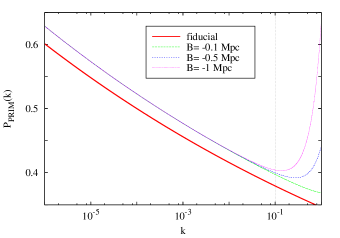
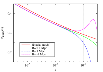
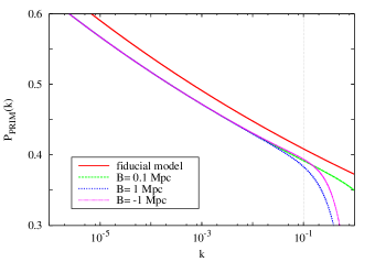
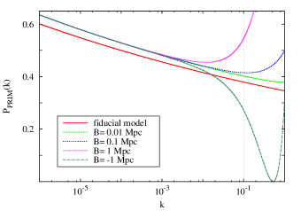
Figures 1, 2 and 3 show the primordial spectra for the different collapse schemes (independent, Newtonian, Wigner), in the case where the proper wavelength associated to the mode is bigger than the Hubble radius at the time of collapse, i.e. $k\ll\mathcal{H}(\eta_{k}^{c})$ [Eqs. (43)], for different values of the collapse parameters $A$ and $B$. The primordial power spectrum of the fiducial model is also shown in each Figure; the value of $A_{s}$ (detailed in the caption of each Fig.) is settled in each case in order to provide the reader a clear idea regarding the differences in the form of the different spectra shown in the plot. For example, in Fig. 1 the fiducial power spectrum could be normalized in such a way that it almost overlaps the primordial spectrum for $B=-0.1$ Mpc. However, for $B=-0.5$ Mpc and $B=-1$ Mpc there is no value of $A_{s}$ that makes both spectra (collapse and fiducial model) overlap. Hereinafter, we discuss the effects of introducing the collapse hypothesis for the different collapse schemes in the primordial power spectrum. The relevant values for $k$ that will affect the prediction of the CMB temperature and polarization anisotropy are $10^{-6}{\rm Mpc}^{-1}<k<10^{-1}{\rm Mpc}^{-1}$. Therefore, we have drawn a vertical line in each Figure, at $k=0.1$ Mpc^-1.

Figure 1 shows no change in the slope of the primordial power spectrum (with respect to the fiducial model one) for the independent scheme in the range $k<0.1$ Mpc^-1 and the considered values of $B$ and the two values of $A$; a notorious deviation in shape from the fiducial one occurs for $k>0.1$ Mpc^-1 . However, we have already mentioned that the relevant values of $l$ that affect the CMB spectrum correspond to $10^{-6}{\rm Mpc}^{-1}<k<10^{-1}{\rm Mpc}^{-1}$, thus we expect no deviation of the CMB temperature spectrum respect the fiducial one for this scheme.

Figure 1: Primordial power spectra for the independent scheme in the case where $k\ll\mathcal{H}(\eta_{k}^{c})$. The power spectrum of the fiducial model is also shown in red. Different values of the collapse time $\eta_{k}^{c}=A/k+B$ are considered, the scalar spectral index $n_{s}=0.96$; Top: $A=-10^{-1}$, Bottom: $A=-10^{-2}$; for both figures $A_{s}=0.39$. The difference in the amplitude between the collapse models and the fiducial model is artificially set to show the functional form of both models.

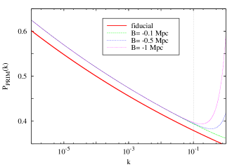
Again, Figure 2 shows no change in the slope of the power spectrum, but unlike the previous case, there is a deviation from the fiducial power spectrum for increasing values of $B$, and this deviation happens within the relevant range of $k$. Furthermore, it should be noted the huge value of $A_{s}$ considered in order to make comparisons between the collapse and fiducial power spectrum. A different value of this parameter with respect to the the value of the standard model could result in a different value for the scale energy of the inflationary period. However, the complete determination of this scale energy depends not only on the temperature fluctuations of the CMB but also on the $B$-mode polarization. As mentioned before, a recent joint paper by the BICEP2/Keck and Planck collaborations concludes that there is no evidence for primordial $B$-modes at low angular multipoles.

Figure 2: Primordial power spectra for the Newtonian collapse scheme in the case where $k\ll\mathcal{H}(\eta_{k}^{c})$. The power spectrum of the fiducial model is also shown in red. Different values of the collapse time $\eta_{k}^{c}=A/k+B$ are considered, the scalar spectral index $n_{s}=0.96$; Top: $A=-10^{-1}$ and $A_{s}=2.8\times 10^{5}$, Bottom: $A=-10^{-3}$ and $A_{s}=3\times 10^{13}$. The difference in the amplitude between the collapse models and the fiducial model is artificially set to show the shape of both models.

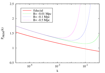
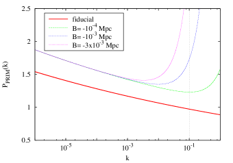
Figure 3 shows the differences in the primordial spectra among different values of $B$ for the two values of $A$ considered and also with respect to the fiducial model for the Wigner’s scheme. It is interesting to note that the deviation with respect to the fiducial model goes to the opposite side that in the Newtonian scheme discussed previously. Furthermore, as in the Newtonian scheme, it was necessary to consider large values of $A_{s}$ in order to make the collapse and fiducial model spectra comparable. Thus, the discussion made for the Newtonian scheme is also valid for this case.

In summary, in this preliminary analysis for the case where $k\ll\mathcal{H}(\eta_{k}^{c})$, we could find values of the collapse parameters ($A$ and $B$) that make the primordial power spectrum of the collapse models to be almost equal to the fiducial primordial power spectrum for the all the schemes considered in this paper. In consequence, we expect that the corresponding CMB spectrum will not deviate much from the fiducial one.

Figure 3: Primordial power spectra for the Wigner collapse scheme in the case where $k\ll\mathcal{H}(\eta_{k}^{c})$. The power spectrum of the fiducial model is also shown in red. Different values of the collapse time $\eta_{k}^{c}=A/k+B$ are considered, the scalar spectral index $n_{s}=0.96$; Top: $A=-10^{-1}$ with $A_{s}=80$, Bottom: $A=-10^{-2}$ with $A_{s}=7000$. The difference in the amplitude between the collapse models and the fiducial model is artificially set to show the functional form of both models.

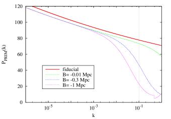
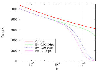
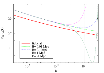
Figures 4, 5 and 6 show the primordial spectra for the different collapse schemes (independent, Newtonian, Wigner) in the case where the proper wavelength associated to the mode is smaller than the Hubble radius at the time of collapse, i.e. $k\gg\mathcal{H}(\eta_{k}^{c})$ [Eqs. (45)] for different values of the collapse parameters $A$ and $B$. The primordial power spectrum of the fiducial model is also shown in each Figure and the value of $A_{s}$ (detailed in the caption of each Figure) is settled in each case in order to provide the reader a clear idea regarding the differences in the form of the different spectra shown in the plot. The relevant values for $k$ that will affect the prediction of the CMB temperature and polarization anisotropy are $10^{-6}{\rm Mpc}^{-1}<k<10^{-1}{\rm Mpc}^{-1}$. Therefore, we have drawn a vertical in each Figure, at $k=0.1$ Mpc^-1. For the independent scheme (Fig. 4), it should be noted that for $A=-10^{2}$ the power spectrum deviates from the fiducial model for increasing values of $B$, however, it is a small change compared to the deviations of other schemes (see Figs. 5 and 6), while for $A=-10^{6}$ there is no difference in the spectrum among different values of $B$. This is due to the fact that for large values of $A$, the value of $z_{k}$ becomes also very large, and therefore the value of $B$ does not affect the final form of the power spectrum. This behavior is similar to the case where the scale factor is exactly de Sitter (see Ref. Landau et al. (2012)).

Figure 4: Primordial power spectra for the independent scheme in the case where $k\gg\mathcal{H}(\eta_{k}^{c})$. The power spectrum of the fiducial model is also shown in red. Different values of the collapse time $\eta_{k}^{c}=A/k+B$ are considered, the scalar spectral index $n_{s}=0.96$; Top: $A=-10^{2}$, Bottom: $A=-10^{6}$, for both figures $A_{s}=0.43$. The difference in the amplitude between the collapse models and the fiducial model is artificially set to show the shape of both models.

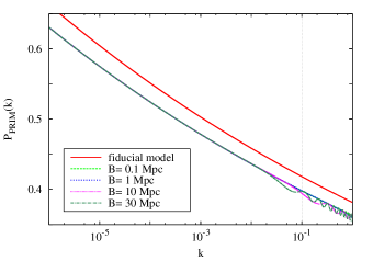
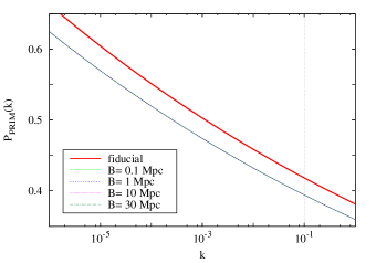
For the Newtonian scheme (Figure 5) it should be mentioned that in both cases ($A=-10^{2}$ and $A=-10^{5}$) considered for increasing values of $B$ the spectrum deviates from the fiducial one for $k>0.01$ Mpc^-1.

Figure 5: Primordial power spectra for the Newtonian collapse scheme in the case where $k\gg\mathcal{H}(\eta_{k}^{c})$. The power spectrum of the fiducial model is also shown in red. Different values of the collapse time $\eta_{k}^{c}=A/k+B$ are considered, the scalar spectral index $n_{s}=0.96$; Top: $A=-10^{2}$ with $A_{s}=0.3$, Bottom: $A=-10^{5}$ with $A_{s}=0.42$. The difference in the amplitude between the collapse models and the fiducial model is artificially set to show the shape of both models.

For the Wigner scheme (Figure 6), it should be mentioned that for increasing values of $B$ the power spectrum deviates more from the fiducial model in both cases ($A=-10^{2}$ and $A=-10^{6}$) for $k>0.005$ Mpc^-1. In summary, increasing the value of $B$ results in a deviation from the fiducial model spectrum; the deviation is more drastically for the Newtonian and Wigner scheme.

Figure 6: Primordial power spectra for the Wigner collapse scheme in the case where $k\gg\mathcal{H}(\eta_{k}^{c})$. The power spectrum of the fiducial model is also shown in red. Different values of the collapse time $\eta_{k}^{c}=A/k+B$ are considered, the scalar spectral index $n_{s}=0.96$; Top: $A=-10^{2}$ with $A_{s}=0.39$, Bottom: $A=-10^{6}$ with $A_{s}=0.21$. The difference in the amplitude between the collapse models and the fiducial model is artificially set to show the shape of both models.

VII Predictions of the collapse schemes on the CMB temperature spectrum

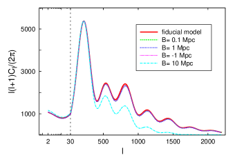
The aim of this section is to show, that introducing the collapse of the inflaton wave function during inflation has observable consequences on the CMB fluctuation spectrum. In this paper, we will limit ourselves to the analysis of the temperature auto-correlation spectrum; however, from a previous analysis of similar models Landau et al. (2012) we might expect that the $E$-mode polarization and temperature-$E$-mode cross correlation will be also modified as a consequence of the collapse hypothesis. As we will see, the effect is different for the three collapse schemes proposed in this paper and it also depends on the value of the time of collapse. This is not a surprise since we have shown in the previous section that there are differences between the primordial power spectrum in each collapse scheme and the standard inflationary model one. We want to stress that, in this paper, we will only perform a preliminary analysis of the CMB spectrum predicted by the collapse models for some particular cases; a complete analysis, including statistical analysis, in which recent CMB data are confronted with the predictions from all collapse schemes, is in progress Piccirilli et al. (2015). In order to perform our analysis, let us define the cosmological parameters of our fiducial model: baryon density in units of the critical density $\Omega_{B}h^{2}=0.02212$, dark matter density in units of the critical density $\Omega_{CDM}h^{2}=0.1187$, Hubble constant in units of ${\rm Mpc^{-1}km\>s^{-1}}$ $H_{0}=67.75$, reionization optical depth, $\tau=0.092$, and the scalar spectral index, $n_{s}=0.96$. These are the best-fit values presented by the Planck collaboration Planck Collaboration et al. (2014b). The value of $A_{s}$ is settled in each case in order to match the maximum of the first Doppler peak with the fiducial model one.

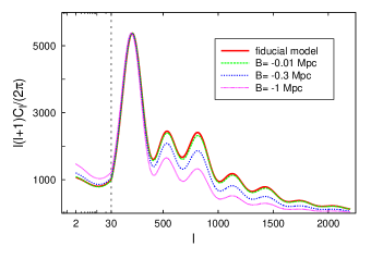
Figs. 7, 8 and 9 show the prediction for the CMB temperature fluctuation spectrum for the independent, Newtonian and Wigner schemes in the case where $k\ll\mathcal{H}(\eta_{k}^{c})$. Let us first analyze the case of the independent scheme; for the two cases shown in this paper ($A=-10^{-1}$ and $A=-10^{-2}$) there is only a very tiny difference between the fiducial spectrum and the one including the self-induce collapse of the inflaton’s wave function. We have calculated the $\chi^{2}$ using the latest release of Planck data, and the difference between the value of the fiducial model and the collapse model is within the expected values for this quantity. In consequence, we expect that any value of $B$ can explain recent observational data.

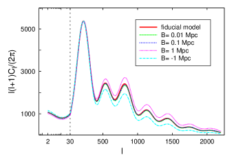
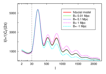
Conversely, Figs. 8 and 9 show large deviations for increasing values of $B$ in the temperature power spectrum respect to the fiducial one. On the other hand, we would like to stress that the values of $A_{s}$ required to match the collapse and the fiducial spectrum are large and, thus, these cases could be severely constrained with future measurements of the $B$-polarization mode.

In such way, we expect that a future statistical analysis using latest Planck data, will allow us to constrain the values of $B$ for the Newtonian and Wigner’s scheme in the case where the collapse occurs when the proper wavelength of the mode is bigger than the Hubble radius.

Figure 7: The temperature auto-correlation (TT) power spectrum for the independent scheme in the case where $k\ll\mathcal{H}(\eta_{k}^{c})$. All models are normalized to the maximum of the first peak of the fiducial model. The power spectrum of the fiducial model is also shown in red. Different values of the collapse time $\eta_{k}^{c}=A/k+B$ are considered, the scalar spectral index $n_{s}=0.96$; Top: $A=-10^{-1}$, Bottom: $A=-10^{-2}$.

Figure 8: The temperature auto-correlation (TT) power spectrum for the Newtonian scheme in the case where $k\ll\mathcal{H}(\eta_{k}^{c})$. All models are normalized to the maximum of the first peak of the fiducial model. The power spectrum of the fiducial model is also shown in red. Different values of the collapse time $\eta_{k}^{c}=A/k+B$ are considered, the scalar spectral index $n_{s}=0.96$; Top: $A=-10^{-1}$, Bottom: $A=-10^{-3}$.

Figure 9: The temperature auto-correlation (TT) power spectrum for the Wigner scheme in the case where $k\ll\mathcal{H}(\eta_{k}^{c})$. All models are normalized to the maximum of the first peak of the fiducial model. The power spectrum of the fiducial model is also shown in red. Different values of the collapse time $\eta_{k}^{c}=A/k+B$ are considered, the scalar spectral index $n_{s}=0.96$; Top: $A=-10^{-1}$, Bottom: $A=-10^{-2}$.

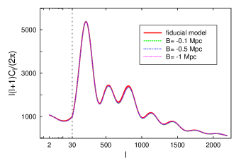
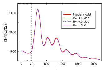
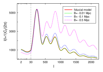
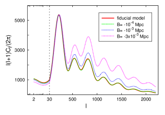
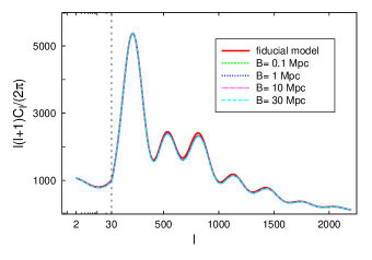
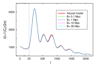
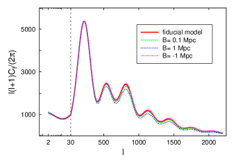
Figures 10, 11 and 12 show the prediction for the temperature fluctuation spectrum for the independent, Newtonian and Wigner schemes in the case where $k\gg\mathcal{H}(\eta_{k}^{c})$. In the independent scheme (Fig. 10), we obtain no changes in the CMB temperature power spectrum for the different values of $B$ considered and only a small difference with respect to the fiducial model (in agreement with Fig 4). Therefore, we expect that any value of $B$ will explain recent observational data for the values of $A$ analyzed in this paper. In the Newtonian and Wigner schemes (Figs. 11 and 12 respectively), for increasing value of $B$ we can observe an increase in the value of the secondary peaks and a decrease of the value at the valleys; the magnitude of the changes depending on the value of $B$, the change is greater for the Wigner scheme. Therefore, we expect that a statistical analysis comparing the model predictions with observational data can give good constraints on the value of $B$ and in consequence on the time of collapse. In particular, from this preliminary analysis, we can expect that the value of $B$ should be smaller than $1$ Mpc in order to fit recent observational data. To get a more stringent bound we need to perform a statistical analysis using Planck and other CMB data and this is left for a forthcoming work Piccirilli et al. (2015). In summary, from the predictions for the CMB temperature power spectrum shown in this section, we can expect that the comparison with recent observational data will constrain the values of $B$ for the Newtonian and Wigner schemes in both cases analyzed in this paper (i.e. when the proper wavelength of the mode is smaller/bigger than the Hubble radius at the time of collapse). In contrast, we can expect that any value of $B$ will explain recent observational data for the independent scheme in the case where $k\gg\mathcal{H}(\eta_{k}^{c})$ and $k\ll\mathcal{H}(\eta_{k}^{c})$. However, we remind the reader that this analysis is valid only for the values of $A$ considered in this section; a complete analysis studying all allowed values of $A$ is in progress Piccirilli et al. (2015).

Figure 10: The temperature auto-correlation (TT) power spectrum for the independent scheme in the case where $k\gg\mathcal{H}(\eta_{k}^{c})$. All models are normalized to the maximum of the first peak of the fiducial model. The power spectrum of the fiducial model is also shown in red. Different values of the collapse time $\eta_{k}^{c}=A/k+B$ are considered, the scalar spectral index $n_{s}=0.96$; Top: $A=-10^{2}$, Bottom: $A=-10^{6}$.

Figure 11: The temperature auto-correlation (TT) power spectrum for the Newtonian scheme in the case where $k\gg\mathcal{H}(\eta_{k}^{c})$. All models are normalized to the maximum of the first peak of the fiducial model. The power spectrum of the fiducial model is also shown in red. Different values of the collapse time $\eta_{k}^{c}=A/k+B$ are considered, the scalar spectral index $n_{s}=0.96$; Top: $A=-10^{2}$, Bottom: $A=-10^{5}$.

Figure 12: The temperature auto-correlation (TT) power spectrum for the Wigner scheme in the case where $k\gg\mathcal{H}(\eta_{k}^{c})$. All models are normalized to the maximum of the first peak of the fiducial model. The power spectrum of the fiducial model is also shown in red. Different values of the collapse time $\eta_{k}^{c}=A/k+B$ are considered, the scalar spectral index $n_{s}=0.96$; Top: $A=-10^{2}$, Bottom: $A=-10^{6}$.

VIII Summary and Conclusions

In this paper, we have calculated the primordial power spectra for the simplest inflationary model, i.e. a single-scalar field in the slow-roll approximation, but taking into account a collapse of the inflaton wave function (for each mode); the motivation for considering an objective collapse is to provide a precise explanation for the emergence of an inhomogeneous and anisotropic universe. Unlike previous works, we have considered a quasi-de Sitter background to perform our calculations. Even though, we have not assumed a particular mechanism for the collapse to happen, we have chosen three different collapse schemes, in which the difference between them is due to the variable that is affected by the collapse and their correlations.

The three collapse schemes induced a modification to the standard scalar power spectrum of the form $P(k)=(\mathcal{C}/\pi^{2})k^{n_{s}-1}Q(|z_{k}|)$, with $n_{s}-1=-2\epsilon_{H}+2\delta_{V}$ and $Q(|z_{k}|)$ a function of the time of collapse $\eta_{k}^{c}$ (recall the definition $z_{k}\equiv k\eta_{k}^{c}$).

Moreover, we have characterized the time of collapse as $\eta_{k}^{c}=A/k+B$. If $B=0$, in all schemes, we can recover an equivalent power spectrum that is, for all practical purposes, indistinguishable from the standard one. The reason for this, is that in this case, $z_{k}=A$ and the dependence of primordial power spectrum with $k$ is the same than in standard inflationary models. The only difference in this case is the relation between $n_{s}$ and the slow-roll parameters of the inflationary model [see Eqs. (37) and (41)]. However, we would like to stress that present constraints on $n_{s}$ (obtained by comparison with observational data) that affect the slow-roll parameters can be fulfilled by our model as well as the standard one, since in both cases the requirement for an efficient inflationary stage is $\epsilon_{V}\simeq\delta_{V}\ll 1$.

On the other hand, by assuming $B\neq 0$, we have found small departures from the standard prediction that are uniquely determined by the collapse proposal; this is in contrast with previous works, in which the introduction of the $B$ parameter was used primarily to depart from an exact scale invariant spectrum. Moreover, given that those works were based on assumptions that led to a power spectrum with an spectral index $n_{s}=1$, one could not tell the precise difference between the dependence on $k$ given purely by the dynamics in the aforementioned background or by the collapse proposal.

The primordial power spectrum for the collapse models obtained in this paper considering $B\neq 0$ has an additional dependence on $k$, which is similar to the one that is obtained in standard inflationary models with a running spectral index. However, as it follows from Eqs. (43) and (45) the dependence on $k$ of the collapse primordial spectrum is different from the standard model one. Additionally, as we have mentioned before, the lowest multipoles of the temperature anisotropy are best fitted by models with $n_{\rm run}\neq 0$ Hinshaw et al. (2013); Ade et al. (2014c).

We have also shown some plots of the primordial spectrum resulting from our schemes for some specific values of the collapse parameters and compared them with the standard inflationary model spectrum. We have considered the case where the associated proper wavelength of the modes is bigger and smaller than the Hubble radius at the time of collapse. Finally, we have shown the effects of introducing a self-induced collapse of the inflaton wave function on the CMB temperature fluctuation spectrum. For this preliminary analysis, most of the collapse models proposed in this paper seem to be good candidates to explain present data of the CMB fluctuation spectrum. In particular, in some cases there are no differences between the prediction of the collapse models with respect to standard inflationary model. However, in other cases, for an increasing value of $B$ (affecting the time of collapse) there are important departures from the standard model prediction. Therefore, by performing a statistical analysis using all present observational data from the CMB (which is left for future work Piccirilli et al. (2015)) we will be able to constrain the value of $B$ and thus the acceptable values for the time of collapse. Finally, we have also shown that some particular cases could be discarded without performing any statistical analysis.

We conclude that a more detailed analysis involving recent observational data can be used to discriminate between the three collapse schemes presented. Nevertheless, from the theoretical point of view, we think that the Wigner collapse scheme should be preferred over the other two schemes since it takes into account the natural correlations between the canonical variables that are present in the pre-collapse vacuum state. The choice of the Wigner distribution to describe these correlations in the present setting is justified by some of its standard properties regarding the “classical limit,” and, by the fact that there is a precise sense in which it is known to encode the correlations in question.

Appendix A Deduction of Eq. (4)

Einstein equations at first order in the perturbations, $\delta G_{0}^{0}=8\pi G\delta T_{0}^{0}$, $\delta G_{i}^{0}=8\pi G\delta T_{i}^{0}$ and $\delta G^{i}_{j}=8\pi G\delta T^{i}_{j}$, are given respectively by

$$\nabla^{2}\Psi-3\mathcal{H}(\mathcal{H}\Phi+\Psi^{\prime})=4\pi G[-\phi_{0}^{\prime 2}\Phi+\phi_{0}^{\prime}\delta\phi^{\prime}+\partial_{\phi}Va^{2}\delta\phi],$$ (46)

$$\partial_{i}(\mathcal{H}\Phi+\Psi^{\prime})=4\pi G\partial_{i}(\phi_{0}^{\prime}\delta\phi),$$ (47)

$$[\Psi^{\prime\prime}+\mathcal{H}(2\Psi+\Phi)^{\prime}+(2\mathcal{H}^{\prime}+\mathcal{H}^{2})\Phi+\textstyle{\frac{1}{2}}\nabla^{2}(\Phi-\Psi)]\delta^{i}_{j}$$

$$- \textstyle{\frac{1}{2}}\partial^{i}\partial_{j}(\Phi-\Psi)=4\pi G[\phi_{0}^{\prime}\delta\phi^{\prime}-\phi_{0}^{\prime 2}\Phi-\partial_{\phi}Va^{2}\delta\phi]\delta^{i}_{j}.$$

The perturbations considered $\Psi,\Phi$ correspond to the gauge-invariant quantities known as the Bardeen potentials; the perturbation $\delta\phi$ and $\delta\phi^{\prime}$ are the gauge invariant perturbations associated to the inflaton field. For the case $i\not=j$ in Eq. (A), together with appropriate boundary conditions (more easily seen in the Fourier transformed version), leads to $\Psi=\Phi$; from now on we will use this result.

Equations (46), (47), (A) above, together with Friedmann equations, can be manipulated to yield the following expression:

$$\nabla^{2}\Psi+\mu\Psi=4\pi G(\omega\delta\phi+\phi_{0}^{\prime}\delta\phi^{\prime}),$$ (49)

where $\mu\equiv\mathcal{H}^{2}-\mathcal{H}^{\prime}$ and $\omega\equiv 3\mathcal{H}\phi_{0}^{\prime}+a^{2}\partial_{\phi}V$. Upon use of the motion equation for $\phi_{0}$ in the slow-roll approximation, i.e. $3\mathcal{H}\phi_{0}^{\prime}+a^{2}\partial_{\phi}V\approx 0$, implies that $\omega\approx 0$. Thus (49) becomes:

$$\nabla^{2}\Psi+\mu\Psi=4\pi G\phi_{0}^{\prime}\delta\phi^{\prime}.$$ (50)

Appendix B Explicit equations of Sec. III

B.1 Equations of Sec. III.2

The mode function $y_{k}(\eta)$ of Eq. (12), can be expressed as $y_{k}(\eta)=\textrm{Re}[y_{k}(\eta)]+i\textrm{Im}[y_{k}(\eta)]$; similarly, the mode function $g_{k}(\eta)$ can be expressed as $g_{k}(\eta)=\textrm{Re}[g_{k}(\eta)]+i\textrm{Im}[g_{k}(\eta)]$ (recall that $g_{k}=y_{k}^{\prime}-\mathcal{H}y_{k}$). Thus, the real and imaginary parts of $y_{k}$ and $g_{k}$ are:

$$\textrm{Re}[y_{k}(\eta)]=\left(\frac{\pi}{4}\right)^{1/2}\frac{\sqrt{-k\eta}}{k^{1/2}}J_{\nu}(-k\eta),$$ (51)

$$\textrm{Im}[y_{k}(\eta)]=\left(\frac{\pi}{4}\right)^{1/2}\frac{\sqrt{-k\eta}}{k^{1/2}}Y_{\nu}(-k\eta),$$ (52)

$$\textrm{Re}[g_{k}(\eta)] = k^{1/2}\left(\frac{\pi}{4}\right)^{1/2}\bigg{(}\frac{-\alpha J_{\nu}(-k\eta)}{\sqrt{-k\eta}}$$ (53)

$$+ \sqrt{-k\eta}J_{\nu+1}(-k\eta)\bigg{)},$$

$$\textrm{Im}[g_{k}(\eta)] = k^{1/2}\left(\frac{\pi}{4}\right)^{1/2}\bigg{(}\frac{-\alpha Y_{\nu}(-k\eta)}{\sqrt{-k\eta}}$$ (54)

$$+ \sqrt{-k\eta}Y_{\nu+1}(-k\eta)\bigg{)},$$

where $\alpha\equiv 1/2+\nu+1/(1-\epsilon_{H})$.

With the previous expressions at hand, we can now compute $\left(\Delta\hat{y}^{R,I}_{\textbf{k}}(\eta_{k}^{c})\right)^{2}_{0}$ and $\left(\Delta\hat{\pi}^{R,I}_{\textbf{k}}(\eta_{k}^{c})\right)^{2}_{0}$ within the independent and Newtonian collapse schemes. The exact form of the quantum uncertainties can be obtained from Eqs. (13), this is

$$\left(\Delta\hat{y}^{R,I}_{\textbf{k}}(\eta_{k}^{c})\right)^{2}_{0} = \frac{L^{3}}{4}|y_{k}(\eta_{k}^{c})|^{2}$$ (55)

$$= \frac{L^{3}\pi|z_{k}|}{16k}\left[J_{\nu}^{2}(|z_{k}|)+Y_{\nu}^{2}(|z_{k}|)\right],$$

$$\left(\Delta\hat{\pi}^{R,I}_{\textbf{k}}(\eta_{k}^{c})\right)^{2}_{0} = \frac{L^{3}}{4}|g_{k}(\eta_{k}^{c})|^{2}=\frac{L^{3}\pi k}{16}$$

$$\times \bigg{[}\left(\frac{-\alpha J_{\nu}(|z_{k}|)}{\sqrt{|z_{k}|}}+\sqrt{z_{k}|}J_{\nu+1}(|z_{k}|)\right)^{2}$$

$$+ \left(\frac{-\alpha Y_{\nu}(|z_{k}|)}{\sqrt{|z_{k}|}}+\sqrt{|z_{k}|}Y_{\nu+1}(|z_{k}|)\right)^{2}\bigg{]},$$

with $z_{k}\equiv k\eta_{k}^{c}$ and $\eta_{k}^{c}$ the time of collapse for each mode. Note that this quantities have the information that the background space-time is quasi-de Sitter

In the case of the Wigner scheme, the explicit formulas characterizing the parameters $\Lambda_{k}(z_{k})$ and $\Theta_{k}(z_{k})$ are:

$$\Lambda_{k} =(2L)^{3/2}\sqrt{\frac{\pi|z_{k}|}{4k}}\left[J_{\nu}^{2}(|z_{k}|)+Y_{\nu}^{2}(|z_{k}|)\right]^{1/2}\bigg{[}S(|z_{k}|)$$

$$- \sqrt{S^{2}(|z_{k}|)-\left(\frac{\pi|z_{k}|}{2}\right)^{2}(J_{\nu}^{2}(|z_{k}|)+Y_{\nu}^{2}(|z_{k}|))^{2}}\bigg{]}^{-1/2},$$

$$\tan 2\Theta_{k} =-\frac{\pi^{2}|z_{k}|}{4}\left[J_{\nu}^{2}(|z_{k}|)+Y_{\nu}^{2}(|z_{k}|)\right]$$

$$\times \left[S(|z_{k}|)-\frac{\pi|z_{k}|}{8}\left(J_{\nu}^{2}(|z_{k}|)+Y_{\nu}^{2}(|z_{k}|)\right)^{2}\right]^{-1}$$

$$\times [-2\nu\left(J_{\nu}^{2}(|z_{k}|)+Y_{\nu}^{2}(|z_{k})\right)+|z_{k}|$$

$$\times \left(J_{\nu}(|z_{k}|)J_{\nu+1}(|z_{k}|)+Y_{\nu}(|z_{k}|)Y_{\nu+1}(|z_{k}|)\right)],$$

where

$$S(|z_{k}|) \equiv 1+\frac{\pi^{2}}{16}\bigg{\{}|z_{k}|^{2}(J_{\nu}^{2}(|z_{k}|)+Y_{\nu}^{2}(|z_{k}|))^{2}$$

$$+ 4\bigg{[}J_{\nu}^{2}(|z_{k}|)+Y_{\nu}^{2}(|z_{k}|)-|z_{k}|(J_{\nu}(|z_{k}|)J_{\nu+1}(|z_{k}|)$$

$$+ Y_{\nu}(|z_{k}|)Y_{\nu+1}(|z_{k}|))\bigg{]}^{2}\bigg{\}}.$$

B.2 Equations of Sec. III.3

In order to deduce Eq. (20), we introduce the quantity $d^{R,I}_{\textbf{k}}\equiv\langle\Theta|\hat{a}_{\textbf{k}}^{R,I}|\Theta\rangle$ that determines the expectation value of the field and momentum operator for the mode k at all times after the collapse. That is, from Eq. (13), we have

$$\langle\hat{\pi}_{\textbf{k}}^{R,I}(\eta)\rangle_{\Theta}=\sqrt{2}\mathcal{R}[g_{k}(\eta)d_{\textbf{k}}^{R,I}],$$ (60)

which corresponds to expectation values at any time after the collapse in the post-collapse state $|\Theta\rangle$. One can then relate the value of $d_{\textbf{k}}^{R,I}$ with the value of the expectation value of the fields operators at the time of collapse $\langle\hat{y}_{\textbf{k}}^{R,I}(\eta_{k}^{c})\rangle_{\Theta}=\sqrt{2}\mathcal{R}[y_{k}(\eta_{k}^{c})d_{\textbf{k}}^{R,I}]$, $\langle\hat{\pi}_{\textbf{k}}^{R,I}(\eta_{k}^{c})\rangle_{\Theta}=\sqrt{2}\mathcal{R}[g_{k}(\eta_{k}^{c})d_{\textbf{k}}^{R,I}]$. Using the latter relations to express $d_{\textbf{k}}^{R,I}$ in terms of the expectation values at the time of collapse and substituting it in (60), we obtain an expression for the expectation value of the momentum field operator in terms of the expectation value at the time of collapse

$$\langle\hat{\pi}_{\textbf{k}}^{R,I}(\eta)\rangle_{\Theta} = F(k\eta,z_{k})\langle\hat{y}_{\textbf{k}}^{R,I}(\eta_{k}^{c})\rangle_{\Theta}$$ (61)

$$+ G(k\eta,z_{k})\langle\hat{\pi}_{\textbf{k}}^{R,I}(\eta_{k}^{c})\rangle_{\Theta},$$

with

$$F(k\eta,z_{k}) \equiv \frac{k\pi}{4}\bigg{\{}\left(\frac{-\alpha Y_{\nu}(|z_{k}|)}{\sqrt{|z_{k}|}}+\sqrt{|z_{k}|}Y_{\nu+1}(|z_{k}|)\right)$$

$$\times \left(\frac{-\alpha J_{\nu}(|k\eta|)}{\sqrt{|k\eta|}}+\sqrt{|k\eta|}J_{\nu+1}(|k\eta|)\right)$$

$$- \left(\frac{-\alpha J_{\nu}(|z_{k}|)}{\sqrt{|z_{k}|}}+\sqrt{|z_{k}|}J_{\nu+1}(|z_{k}|)\right)$$

$$\times \left(\frac{-\alpha Y_{\nu}(|k\eta|)}{\sqrt{|k\eta|}}+\sqrt{|k\eta|}Y_{\nu+1}(|k\eta|)\right)\bigg{\}},$$

$$G(k\eta,z_{k})\equiv\frac{\pi\sqrt{|z_{k}|}}{4}\bigg{\{}J_{\nu}(|z_{k}|)$$ (63)

$$\times \left[\frac{-\alpha Y_{\nu}(|k\eta|)}{\sqrt{|k\eta|}}+\sqrt{|k\eta|}Y_{\nu+1}(|k\eta|)\right]$$

$$- Y_{\nu}(|z_{k}|)\left[\frac{-\alpha J_{\nu}(|k\eta|)}{\sqrt{|k\eta|}}+\sqrt{|k\eta|}J_{\nu+1}(|k\eta|)\right]\bigg{\}}.$$

Furthermore, given Eqs. (61) and (15), we can find the curvature perturbation in the longitudinal gauge within the three collapse schemes.

For the independent scheme the curvature perturbation is:

$$\Psi_{\textbf{k}}^{\text{ind}}(\eta)=\frac{\sqrt{L^{3}\pi\epsilon_{V}}H}{2^{5/2}M_{P}k^{2}}$$ (64)

$$\times \bigg{\{}F(k\eta,z_{k})X_{\textbf{k},1}\sqrt{\frac{|z_{k}|}{k}}\left[J_{\nu}^{2}(|z_{k}|)+Y_{\nu}^{2}(|z_{k}|)\right]^{1/2}$$

$$+ G(k\eta,z_{k})X_{\textbf{k},2}\sqrt{k}$$

$$\times \bigg{[}\left(\frac{-\alpha J_{\nu}(|z_{k}|)}{\sqrt{|z_{k}|}}+\sqrt{|z_{k}|}J_{\nu+1}(|z_{k}|)\right)^{2}$$

$$+ \left(\frac{-\alpha Y_{\nu}(|z_{k}|)}{\sqrt{|z_{k}|}}+\sqrt{|z_{k}|}Y_{\nu+1}(|z_{k}|)\right)^{2}\bigg{]}^{1/2}\bigg{\}}.$$

Meanwhile, for the Newtonian scheme we have

$$\Psi_{\textbf{k}}^{\text{newt}}(\eta) = \frac{\sqrt{L^{3}\pi\epsilon_{V}}H}{2^{5/2}M_{P}k^{2}}G(k\eta,z_{k})X_{\textbf{k},2}\sqrt{k}$$ (65)

$$\times \bigg{[}\left(\frac{-\alpha J_{\nu}(|z_{k}|)}{\sqrt{|z_{k}|}}+\sqrt{|z_{k}|}J_{\nu+1}(|z_{k}|)\right)^{2}$$

$$+ \left(\frac{-\alpha Y_{\nu}(|z_{k}|)}{\sqrt{|z_{k}|}}+\sqrt{|z_{k}|}Y_{\nu+1}(|z_{k}|)\right)^{2}\bigg{]}^{1/2}$$

and finally for the Wigner scheme

$$\Psi_{\textbf{k}}^{\text{wig}}(\eta) = \sqrt{\frac{\epsilon_{V}}{2}}\frac{H}{M_{P}k^{2}}\Lambda_{k}[F(k\eta,z_{k})\cos\Theta_{k}$$ (66)

$$+ kG(k\eta,z_{k})\sin\Theta_{k}]X_{\textbf{k}},$$

with $X_{\textbf{k}}\equiv x_{\textbf{k}}^{R}+ix_{\textbf{k}}^{I}$.

B.3 Definitions of the functions $M(|z_{k}|)$, $N(|z_{k}|)$ and $W(|z_{k}|)$

$$M(|z_{k}|) \equiv -\sqrt{|z_{k}|}\bigg{[}\frac{-\alpha J_{\nu}(|z_{k}|)}{\sqrt{|z_{k}|}}+\sqrt{|z_{k}|}J_{\nu+1}(|z_{k}|)\bigg{]}$$ (67)

$$\times \left[J_{\nu}^{2}(|z_{k}|)+Y_{\nu}^{2}(|z_{k}|)\right]^{1/2},$$

$$N(|z_{k}|)\equiv\sqrt{|z_{k}|}J_{\nu}(|z_{k}|)$$ (68)

$$\times \bigg{[}\left(\frac{-\alpha J_{\nu}(|z_{k}|)}{\sqrt{|z_{k}|}}+\sqrt{|z_{k}|}J_{\nu+1}(|z_{k}|)\right)^{2}$$

$$+ \left(\frac{-\alpha Y_{\nu}(|z_{k}|)}{\sqrt{|z_{k}|}}+\sqrt{|z_{k}|}Y_{\nu+1}(|z_{k}|)\right)^{2}\bigg{]}^{1/2},$$

$$W(|z_{k}|)\equiv\frac{2k^{1/2}}{\pi^{1/2}L^{3/2}}$$ (69)

$$\times \bigg{[}-\bigg{(}\frac{-\alpha J_{\nu}(|z_{k}|)}{\sqrt{|z_{k}|}}+\sqrt{|z_{k}|}J_{\nu+1}(|z_{k}|)\bigg{)}\Lambda_{k}\cos\Theta_{k}$$

$$+ \sqrt{|z_{k}|}J_{\nu}(|z_{k}|)\Lambda_{k}\sin\Theta_{k}\bigg{]}.$$

Appendix C Equations of Sec. IV

The explicit expressions for $|a_{lm}|^{2}_{\text{ML}}$ can be found by substituting $\mathcal{R}_{k}$, given in Eq. (23) into Eq. (28), and then making the identification $|a_{lm}|^{2}_{\text{ML}}=\overline{|a_{lm}|^{2}}$

$$|a_{lm}|^{2\text{$$ ind}}_{\text{ML}}=16\pi^{2}\frac{\mathcal{C}}{L^{3}}\sum_{\textbf{k},\textbf{k}^{\prime}}\frac{j_{l}(kR_{D})j_{l}(k^{\prime}R_{D})}{k^{3/2}k^{\prime 3/2}}$$ (70)

$$\times Y_{lm}^{\star}(\hat{k})Y_{lm}(\hat{k}^{\prime})T(k)T(k^{\prime})\bigg{(}M(|z_{k}|)M(|z_{k^{\prime}}|)\overline{X_{\textbf{k},1}X_{\textbf{k}^{\prime},1}^{\star}}$$

$$+ N(|z_{k}|)N(|z_{k^{\prime}}|)\overline{X_{\textbf{k},2}X_{\textbf{k}^{\prime},2}^{\star}}\bigg{)}(kk^{\prime})^{3/2-\nu},$$

$$|a_{lm}|^{2\text{$$ newt}}_{\text{ML}}={16\pi^{2}}\frac{\mathcal{C}}{L^{3}}\sum_{\textbf{k},\textbf{k}^{\prime}}\frac{j_{l}(kR_{D})j_{l}(k^{\prime}R_{D})}{k^{3/2}k^{\prime 3/2}}$$ (71)

$$\times Y_{lm}^{\star}(\hat{k})Y_{lm}(\hat{k}^{\prime})T(k)T(k^{\prime})N(|z_{k}|)N(|z_{k^{\prime}}|)$$

$$\times \overline{X_{\textbf{k},2}X_{\textbf{k}^{\prime},2}^{\star}}(kk^{\prime})^{3/2-\nu},$$

$$|a_{lm}|^{2\text{$$ wig}}_{\text{ML}}={16\pi^{2}}\frac{\mathcal{C}}{L^{3}}\sum_{\textbf{k},\textbf{k}^{\prime}}\frac{j_{l}(kR_{D})j_{l}(k^{\prime}R_{D})}{k^{3/2}k^{\prime 3/2}}$$ (72)

$$\times Y_{lm}^{\star}(\hat{k})Y_{lm}(\hat{k}^{\prime})T(k)T(k^{\prime})$$

$$\times W(|z_{k}|)W(|z_{k^{\prime}}|)\overline{X_{\textbf{k}}X_{\textbf{k}^{\prime}}^{\star}}(kk^{\prime})^{3/2-\nu},$$

with

$$\mathcal{C}\equiv\frac{\pi}{M_{P}^{2}\epsilon_{H}}\left(2^{\nu-11/2}\Gamma(\nu-1)H|\eta|^{3/2-\nu}\right)^{2},$$ (73)

where we used the fact that in slow-roll inflation $\epsilon_{V}\simeq\epsilon_{H}$.

Appendix D On the meaning of the power spectrum within the collapse proposal

In order to obtain the power spectrum in the traditional inflationary scenario one needs to compute the quantum two-point correlation function. That is, if $\hat{\Psi}$ represents the quantum operator associated to the metric perturbation, then the (scalar) power spectrum is obtained from

$$\langle 0|\hat{\Psi}_{\textbf{k}}\hat{\Psi}_{\textbf{k}^{\prime}}|0\rangle=\frac{2\pi^{2}}{k^{3}}P(k)\delta(\textbf{k}-\textbf{k}^{\prime})$$ (74)

On the other hand, let us recall that in general, the definition of the power spectrum is given in terms of $\Psi_{\textbf{k}}$, i.e. a classical stochastic field not a quantum operator. Therefore, the standard approach is based on the identification

$$\langle 0|\hat{\Psi}_{\textbf{k}}\hat{\Psi}_{\textbf{k}^{\prime}}|0\rangle=\overline{\Psi_{\textbf{k}}\Psi_{\textbf{k}^{\prime}}}$$ (75)

with $\overline{\Psi_{\textbf{k}}\Psi_{\textbf{k}^{\prime}}}$ denoting an average over an ensemble of classical stochastic fields. The justification for the relation above relies on arguments based on decoherence and the squeezing nature of the evolved vacuum state Grishchuk and Sidorov (1990); Kiefer and Polarski (2009) (although we do not subscribe to such arguments for the reasons exposed in Landau et al. (2013); Sudarsky (2011)). Nevertheless, the explanation about the fact that a single outcome or realization $\Psi_{\textbf{k}}$ has emerged is incomplete.

Therefore, in order to show explicitly the manner in which we can obtain an equivalent power spectrum within the collapse proposal, we start by focusing on the temperature anisotropies of the CMB observed today on the celestial two-sphere and its relation to the scalar metric perturbation $\Psi$, which can be approximated by

$$\frac{\delta T}{T_{0}}(\theta,\varphi)\simeq\frac{1}{3}\Psi.$$ (76)

On the other hand, the observational data are described in terms of the coefficients $a_{lm}$ of the multipolar series expansion

$$\begin{split}\frac{\delta T}{T_{0}}(\theta,\varphi)=\sum_{lm}a_{lm}Y_{lm}(\theta,\varphi),\\ a_{lm}=\int\frac{\delta T}{T_{0}}(\theta,\varphi)Y^{*}_{lm}(\theta,\varphi)d\Omega,\end{split}$$ (77)

here $\theta$ and $\varphi$ are the coordinates on the celestial two-sphere, with $Y_{lm}(\theta,\varphi)$ as the spherical harmonics.

The value for the quantities $a_{lm}$ are then given by

$$a_{lm}=\frac{4\pi i^{l}}{3}\int\frac{d^{3}{k}}{(2\pi)^{3}}j_{l}(kR_{D})Y_{lm}^{*}(\hat{k})T(k)\Psi_{\vec{k}},$$ (78)

with $j_{l}(kR_{D})$ as the spherical Bessel function of order $l$ and $R_{D}$ is the comoving radius of the last scattering surface. We have explicitly included the modifications associated with latetime physics encoded in the transfer functions $T(k)$. The metric perturbation $\Psi_{\textbf{k}}$ is the primordial curvature perturbation.

Now, the problem is that, if we compute the expectation value of the right-hand side (i.e., identifying $\langle\hat{\Psi}\rangle=\Psi$) in the vacuum state $|0\rangle$, we obtain 0, while it is clear that for any given $l,m$, the measured value of this quantity is not 0. That is, if we rely in this case on the one-point function and the standard identification of quantum averages with classical ensemble average, we find a large conflict between expectation and observation. Nevertheless, in the standard approach somehow (e.g. by invoking decoherence, squeezing of the vacuum, many-world interpretation of quantum mechanics, etc.) occurs the transition $\hat{\Psi}_{\textbf{k}}\to\Psi_{\textbf{k}}=Ae^{i\alpha_{\textbf{k}}}$ with $\alpha_{\textbf{k}}$ a random phase and $A$ is identified with the quantum uncertainty of $\hat{\Psi}_{\textbf{k}}$, i.e. $A^{2}=\langle 0|\hat{\Psi}_{\textbf{k}}^{2}|0\rangle$, but the random nature of $\Psi_{\textbf{k}}$ remains unclear.

In our approach, the random nature comes directly from the stochastic aspects of the quantum dynamical-reduction, i.e. from the self-induced collapse. Thus, using Eq. (15) in Eq. (78) we obtain

$$a_{lm} = \frac{4\pi i^{l}}{3}\int\frac{d^{3}{k}}{(2\pi)^{3}}j_{l}(kR_{D})Y_{lm}^{*}(\hat{k})\Delta(k)\Psi_{\textbf{k}}$$

$$= \frac{4\pi i^{l}}{3}\sqrt{\frac{\epsilon_{H}}{2}}\frac{H}{M_{P}}\int\frac{d^{3}{k}}{(2\pi)^{3}}j_{l}(kR_{D})Y_{lm}^{*}(\hat{k})T(k)\frac{\langle\hat{\pi}_{\textbf{k}}\rangle}{k^{2}}.$$

The previous expression shows how the expectation value of the momentum field in the post-collapse state acts as a source for the coefficients $a_{lm}$.

Furthermore, the angular power spectrum is defined by

$$C_{l}=\frac{1}{2l+1}\sum_{m}|a_{lm}|^{2}.$$ (80)

For the reasons presented in Sec. IV, we can identify the observed value $|a_{lm}|^{2}$ with the most likely value of $|a_{lm}|^{2}_{ML}$ and in turn, assume that the most likely value coincides approximately with the average $\overline{|a_{lm}|^{2}}$. Thus, in our approach, the observed $C_{l}$ coincides with

$$C_{l}\simeq\frac{1}{2l+1}\sum_{m}\overline{|a_{lm}|^{2}}.$$ (81)

From Eq. (D) we obtain

$$\overline{|a_{lm}|^{2}} = \left(\frac{4\pi}{3}\right)^{2}\int\frac{d^{3}{k}d^{3}{k^{\prime}}}{(2\pi)^{6}}j_{l}(kR_{D})j_{l}(k^{\prime}R_{D})$$

$$\times Y_{lm}^{*}(\hat{k})Y_{lm}(\hat{k}^{\prime})T(k)T(k^{\prime})\overline{\Psi_{\textbf{k}}\Psi_{\textbf{k}^{\prime}}}$$

$$= \left(\frac{4\pi}{3}\right)^{2}\int\frac{d^{3}{k}d^{3}{k^{\prime}}}{(2\pi)^{6}}j_{l}(kR_{D})j_{l}(k^{\prime}R_{D})$$

$$\times Y_{lm}^{*}(\hat{k})Y_{lm}(\hat{k}^{\prime})T(k)T(k^{\prime})\bigg{[}\frac{\epsilon}{2}\frac{H^{2}}{M_{P}^{2}}\overline{\frac{\langle\hat{\pi}_{\textbf{k}}\rangle\langle\hat{\pi}_{\textbf{k}^{\prime}}\rangle}{k^{2}k^{{}^{\prime}2}}}\bigg{]}.$$

Consequently using the generic definition of the power spectrum [i.e. not relying on the identification (75)]

$$\overline{\Psi_{\textbf{k}}\Psi_{\textbf{k}^{\prime}}}\equiv\frac{2\pi^{2}}{k^{3}}P(k)\delta(\textbf{k}-\textbf{k}^{\prime}),$$ (83)

and also using Eq. (D), the power spectrum, associated to $\Psi_{\textbf{k}}$, in our approach is given by

$$P(k)=\frac{\epsilon}{2}\frac{H^{2}}{M_{P}^{2}}\overline{\langle\hat{\pi}_{\textbf{k}}(\eta)\rangle\langle\hat{\pi}_{\textbf{k}^{\prime}}(\eta)\rangle}.$$ (84)

The quantity $\overline{\langle\hat{\pi}_{\textbf{k}}(\eta)\rangle\langle\hat{\pi}_{\textbf{k}^{\prime}}(\eta)\rangle}$ is obtained by using Eq. (20) in the limit $-k\eta\to 0$, i.e. when the proper wavelength of the modes of interest are bigger than the Hubble radius, but taking into account that Eq. (20) is different for each collapse scheme.

References

- Perez et al. (2005) A. Perez, H. Sahlmann, and D. Sudarsky, Classical and Quantum Gravity 23, 2317 (2005), eprint gr-qc/0508100.
- Sudarsky (2011) D. Sudarsky, International Journal of Modern Physics D 20, 509 (2011), eprint 0906.0315.
- de Unánue and Sudarsky (2008) A. de Unánue and D. Sudarsky, Physical Review D 78, 043510 (2008), eprint arXiv:0801.4702.
- León and Sudarsky (2010) G. León and D. Sudarsky, Classical and Quantum Gravity 27, 225017 (2010), eprint 1003.5950.
- Diez-Tejedor and Sudarsky (2012) A. Diez-Tejedor and D. Sudarsky, JCAP 7, 045 (2012), eprint 1108.4928.
- León et al. (2011) G. León, A. De Unánue, and D. Sudarsky, Classical and Quantum Gravity 28, 155010 (2011), eprint 1012.2419.
- Landau et al. (2012) S. J. Landau, C. G. Scóccola, and D. Sudarsky, Physical Review D 85, 123001 (2012), eprint 1112.1830.
- Landau et al. (2013) S. Landau, G. León, and D. Sudarsky, Physical Review D 88, 023526 (2013), eprint 1107.3054.
- León et al. (2014) G. León, S. J. Landau, and M. P. Piccirilli, Phys. Rev. D 90, 083525 (2014), eprint 1410.1562.
- Cañate et al. (2013) P. Cañate, P. Pearle, and D. Sudarsky, Phys.Rev. D 87, 104024 (2013), eprint 1211.3463.
- Penrose (1996) R. Penrose, Gen.Rel.Grav. 28, 581 (1996).
- Diosi (1987) L. Diosi, Phys.Lett. A120, 377 (1987).
- Diosi (1989) L. Diosi, Phys.Rev. A40, 1165 (1989).
- Ghirardi et al. (1986) G. Ghirardi, A. Rimini, and T. Weber, Phys.Rev. D34, 470 (1986).
- Pearle (1989) P. M. Pearle, Phys.Rev. A39, 2277 (1989).
- Bassi and Ghirardi (2003) A. Bassi and G. C. Ghirardi, Phys.Rept. 379, 257 (2003), eprint quant-ph/0302164.
- Bassi et al. (2013) A. Bassi, K. Lochan, S. Satin, T. P. Singh, and H. Ulbricht, Reviews of Modern Physics 85, 471 (2013), eprint 1204.4325.
- Kiefer and Polarski (2009) C. Kiefer and D. Polarski, Adv. Sci. Lett. 2, 164 (2009), eprint 0810.0087.
- Grishchuk and Sidorov (1990) L. Grishchuk and Y. Sidorov, Phys. Rev. D 42, 3413 (1990).
- Martin (2008) J. Martin, in Inflationary Cosmology, edited by M. Lemoine, J. Martin, and P. Peter (2008), vol. 738 of Lecture Notes in Physics, Berlin Springer Verlag, p. 193, eprint 0704.3540.
- Mukhanov (2005) V. Mukhanov, Physical Foundations of Cosmology (Cambridge University Press, New York, 2005).
- Adler (2001) S. L. Adler, eprint arXiv:quant-ph/0112095 (2001), eprint quant-ph/0112095.
- Schlosshauer (2004) M. Schlosshauer, Rev. Mod. Phys. 76, 1267 (2004), eprint quant-ph/0312059.
- Kent (1990) A. Kent, International Journal of Modern Physics A 5, 1745 (1990), eprint gr-qc/9703089.
- Stapp (2002) H. P. Stapp, Canadian Journal of Physics 80, 1043 (2002), eprint quant-ph/0110148.
- Bedingham (2011) D. J. Bedingham, Foundations of Physics 41, 686 (2011), eprint 1003.2774.
- Pearle (2015) P. Pearle, Phys. Rev. D91, 105012 (2015), eprint 1412.6723.
- Ade et al. (2014a) P. Ade et al. (Planck), Astron.Astrophys. 571, A15 (2014a), eprint 1303.5075.
- Bennett et al. (2013) C. L. Bennett, D. Larson, J. L. Weiland, N. Jarosik, G. Hinshaw, N. Odegard, K. M. Smith, R. S. Hill, B. Gold, M. Halpern, et al., Astrophysical Journal Supplement 208, 20 (2013), eprint 1212.5225.
- Das et al. (2014a) S. Das et al., JCAP 1404, 014 (2014a), eprint 1301.1037.
- Reichardt et al. (2012) C. Reichardt, L. Shaw, O. Zahn, K. Aird, B. Benson, et al., Astrophys.J. 755, 70 (2012), eprint 1111.0932.
- Diez-Tejedor et al. (2012) A. Diez-Tejedor, G. Leon, and D. Sudarsky, Gen.Rel.Grav. 44, 2965 (2012), eprint 1106.1176.
- Martin et al. (2012) J. Martin, V. Vennin, and P. Peter, Phys.Rev. D86, 103524 (2012), eprint 1207.2086.
- Das et al. (2013) S. Das, K. Lochan, S. Sahu, and T. Singh, Phys.Rev. D88, 085020 (2013), eprint 1304.5094.
- Das et al. (2014b) S. Das, S. Sahu, S. Banerjee, and T. Singh, Phys.Rev. D90, 043503 (2014b), eprint 1404.5740.
- Isham (1992) C. Isham (1992), eprint gr-qc/9210011.
- Ade et al. (2014b) P. A. R. Ade et al. (BICEP2), Phys. Rev. Lett. 112, 241101 (2014b), eprint 1403.3985.
- Mortonson and Seljak (2014) M. J. Mortonson and U. Seljak, JCAP 10, 035 (2014), eprint 1405.5857.
- Flauger et al. (2014) R. Flauger, J. C. Hill, and D. N. Spergel, JCAP 8, 039 (2014), eprint 1405.7351.
- Liu et al. (2014) H. Liu, P. Mertsch, and S. Sarkar, Astrophys.J. 789, L29 (2014), eprint 1404.1899.
- Planck Collaboration et al. (2014a) Planck Collaboration, R. Adam, P. A. R. Ade, N. Aghanim, M. Arnaud, J. Aumont, C. Baccigalupi, A. J. Banday, R. B. Barreiro, J. G. Bartlett, et al., ArXiv e-prints (2014a), eprint 1409.5738.
- Ade et al. (2015) P. Ade et al. (BICEP2, Planck), Phys. Rev. Lett. 114, 101301 (2015), eprint 1502.00612.
- Markkanen et al. (2015) T. Markkanen, S. Rasanen, and P. Wahlman, Phys. Rev. D91, 084064 (2015), eprint 1407.4691.
- Brandenberger et al. (1993) R. H. Brandenberger, H. Feldman, and V. F. Mukhanov, pp. 19–30 (1993), eprint astro-ph/9307016.
- Leon and Bengochea (2015) G. Leon and G. R. Bengochea (2015), eprint 1502.04907.
- Deruelle and Mukhanov (1995) N. Deruelle and V. F. Mukhanov, Phys.Rev. D52, 5549 (1995), eprint gr-qc/9503050.
- Kinney (2005) W. H. Kinney, Phys.Rev. D72, 023515 (2005), eprint gr-qc/0503017.
- Hinshaw et al. (2013) G. Hinshaw, D. Larson, E. Komatsu, D. N. Spergel, C. L. Bennett, J. Dunkley, M. R. Nolta, M. Halpern, R. S. Hill, N. Odegard, et al., Astrophysical Journal Supplement 208, 19 (2013), eprint 1212.5226.
- Ade et al. (2014c) P. A. R. Ade et al. (Planck), Astron. Astrophys. 571, A16 (2014c), eprint 1303.5076.
- Planck Collaboration et al. (2015) Planck Collaboration, P. A. R. Ade, N. Aghanim, M. Arnaud, F. Arroja, M. Ashdown, J. Aumont, C. Baccigalupi, M. Ballardini, A. J. Banday, et al., ArXiv e-prints (2015), eprint 1502.02114.
- Piccirilli et al. (2015) M. P. Piccirilli, G. Leon, and S. J. Landau, In preparation (2015).
- Planck Collaboration et al. (2014b) Planck Collaboration, P. A. R. Ade, N. Aghanim, C. Armitage-Caplan, M. Arnaud, M. Ashdown, F. Atrio-Barandela, J. Aumont, C. Baccigalupi, A. J. Banday, et al., Astronomy and Astrophysics 571, A16 (2014b), eprint 1303.5076.