Abstract

Inference and learning of graphical models are both well-studied problems in statistics and machine learning that have found many applications in science and engineering. However, exact inference is intractable in general graphical models, which suggests the problem of seeking the best approximation to a collection of random variables within some tractable family of graphical models. In this paper, we focus on the class of planar Ising models, for which exact inference is tractable using techniques of statistical physics. Based on these techniques and recent methods for planarity testing and planar embedding, we propose a simple greedy algorithm for learning the best planar Ising model to approximate an arbitrary collection of binary random variables (possibly from sample data). Given the set of all pairwise correlations among variables, we select a planar graph and optimal planar Ising model defined on this graph to best approximate that set of correlations. We demonstrate our method in simulations and for the application of modeling senate voting records.

1 Introduction

Graphical models are widely used to represent the statistical relations among a set of random variables (Lauritzen, 1996; MacKay, 2003). Nodes of the graph correspond to random variables and edges of the graph represent statistical interactions among the variables. The problems of inference and learning on graphical models arise in many practical applications. The problem of inference is to deduce certain statistical properties (such as marginal probabilities, modes etc.) of a given set of random variables whose graphical model is known. It has wide applications in areas such as error correcting codes, statistical physics and so on. The problem of learning on the other hand is to deduce the graphical model of a set of random variables given statistics (possibly from samples) of the random variables. Learning is also a widely encountered problem in areas such as biology, anthropology and so on.

The Ising model, a class of binary-variable graphical models with pairwise interactions, has been studied by physicists as a simple model of order-disorder transitions in magnetic materials (Onsager, 1944). Remarkably, it was found that in the special case of an Ising model with zero-mean $\{-1,+1\}$ binary random variables and pairwise interactions defined on a planar graph, calculation of the partition function (which is closely tied to inference) is tractable, essentially reducing to calculation of a matrix determinant (Kac and Ward, 1952; Sherman, 1960; Kasteleyn, 1963; Fisher, 1966). These methods have been used in machine learning (Schraudolph and Kamenetsky, 2008; Globerson and Jaakkola, 2007).

We address the problem of approximating a collection of binary random variables (given their pairwise marginal distributions) by a zero-mean planar Ising model. We also consider the related problem of selecting a non-zero mean Ising model defined on an outer-planar graph (these models are also tractable, being essentially equivalent to a zero-field model on a related planar graph).

There has been a great deal of work on learning graphical models. Much of these have focused on learning over the class of thin graphical models (Deshpande et al., 2001; Bach and Jordan, 2001; Karger and Srebro, 2001; Shahaf et al., 2009) for which inference is tractable by converting the model to a junction tree. The simplest case of this is learning tree models (treewidth one graphs) for which it is tractable to find the best tree model by reduction to a max-weight spanning tree problem (Chow and Liu, 1968). However, the problem of finding the best bounded-treewidth model is NP-hard for treewidths greater than two (Karger and Srebro, 2001), and so heuristic methods are used to select the graph structure (Deshpande et al., 2001; Karger and Srebro, 2001). Another popular method is to use convex optimization of the log-likelihood penalized by $\ell_{1}$ norm of parameters of the graphical model so as to promote sparsity (Banerjee et al., 2008; Lee et al., 2006). To go beyond low-treewidth graphs, such methods either focus on Gaussian graphical models or adopt a tractable approximation of the likelihood. Other methods learn only the graph structure itself (Ravikumar et al., 2010; Abbeel et al., 2006) and are often able to demonstrate asymptotic correctness of this estimate under appropriate conditions.

In contrast to existing approaches, this paper explores planarity as an alternative restriction on the model class to both make learning tractable and to offer a qualitatively different graph topology in which the number of edges learned is linear in the number of variables.

2 Preliminaries

In this section, we develop our notation and briefly review the necessary background theory.

2.1 Divergence and Likelihood

Suppose we want to calculate how well a probability distribution $Q$ approximates another probability distribution $P$ (on the same sample space $\chi$). For any two probability distributions $P$ and $Q$ on some sample space $\chi$, we denote by $D(P,Q)$ the Kullback-Leibler divergence (or relative entropy) between $P$ and $Q$ as $D(P,Q)=\sum_{x\in\chi}P(x)\log\frac{P(x)}{Q(x)}$. The log-likelihood function is defined as $LL(P,Q)=\sum_{x\in\chi}P(x)\log Q(x)$. The probability distribution in a family $\mathcal{F}$ that maximizes the log-likelihood of a probability distribution $P$ is called the maximum-likelihood estimate of $P$ in $\mathcal{F}$, and this is equivalent to the minimum-divergence projection of $P$ to $\mathcal{F}$, so that $P_{\mathcal{F}}=\operatorname*{arg\,max}_{Q\in\mathcal{F}}LL(P,Q)=\operatorname*{arg\,min}_{Q\in\mathcal{F}}D(P,Q)$.

2.2 Graphical Models and The Ising Model

We will be dealing with binary random variables throughout the paper. We write $P(x)$ to denote the probability distribution of a collection of random variables $x=(x_{1},\dots,x_{n})$. Unless otherwise stated, we work with undirected graphs $G=(V,E)$ with vertex (or node) set $V$ and edges $\{i,j\}\in E\subset{V\choose 2}$. For vertices $i,j\in V$ we write $G+ij$ to denote the graph $(V,E\cup\{i,j\})$. A pairwise graphical model is a probability distribution $P(x)=P(x_{1},\dots,x_{n})$ that is defined on a graph $G=(V,E)$ with vertices $V=\{1,..,n\}$ as

$$\begin{split}P(x)&\propto\quad\prod_{i\in V}\psi_{i}(x_{i})\prod_{\{i,j\}\in E}\psi_{ij}(x_{i},x_{j})\\ &\propto\quad\exp\biggr{\{}\sum_{i\in V}f_{i}(x_{i})+\sum_{\{i,j\}\in E}f_{ij}(x_{i},x_{j})\biggr{\}}\end{split}$$ (1)

where $\psi_{i},\psi_{ij}\geq 0$ are non-negative node and edge compatibility functions. For positive $\psi$’s, we may also represent $P(x)$ as a Gibbs distribution with potentials $f_{i}=\log\psi_{i}$ and $f_{ij}=\log\psi_{ij}$.

Definition 1.

An Ising model on binary random variables $x=(x_{1},\dots,x_{n})$ and graph $G=(V,E)$ is the probability distribution defined by

$$P(x) =\frac{1}{Z(\theta)}\exp\biggr{\{}\sum_{i\in V}\theta_{i}x_{i}+\!\!\!\sum_{\{i,j\}\in E}\!\!\theta_{ij}x_{i}x_{j}\biggr{\}},$$

$$Z(\theta) =\sum_{x}\exp\biggr{\{}\sum_{i\in V}\theta_{i}x_{i}+\!\!\!\sum_{\{i,j\}\in E}\!\!\theta_{ij}x_{i}x_{j}\biggr{\}},$$

where $x_{i}\in\{-1,1\}$. The partition function $Z(\theta)$ serves to normalize the probability distribution.

Formally, this defines an exponential family $P_{\theta}(x)=\exp\{\theta^{T}\phi(x)-\Phi(\theta)\}$ (Barndorff-Nielsen, 1979; Wainwright and Jordan, 2008) based on sufficient statistics $(\phi_{i}(x)=x_{i},i\in V)$ and $(\phi_{ij}(x)=x_{i}x_{j},\{i,j\}\in E)$, parameters $(\theta_{i},i\in V)$ and $(\theta_{ij},\{i,j\}\in E)$ and moment parameters $(\mu_{i}=\mathbb{E}[x_{i}],i\in V)$ and $(\mu_{ij}=\mathbb{E}[x_{i}x_{j}],\{i,j\}\in E)$. The function $\Phi(\theta)=\log Z(\theta)$ is a convex function of $\theta$ and has the moment generating properties: $\nabla\Phi(\theta)=\mathbb{E}_{\theta}[\phi(x)]=\mu$ and $\nabla^{2}\Phi(\theta)=\mathbb{E}_{\theta}[(\phi(x)-\mu)(\phi(x)-\mu)^{T}]$.

In fact, any pairwise graphical model among binary variables can be represented as an Ising model:

$$\theta_{i} =\tfrac{1}{2}\sum_{x_{i}}x_{i}f_{i}(x_{i})+\tfrac{1}{4}\sum_{\{i,j\}\in E}\sum_{x_{i},x_{j}}x_{i}f_{ij}(x_{i},x_{j}),$$

$$\theta_{ij} =\tfrac{1}{4}\sum_{x_{i},x_{j}}x_{i}x_{j}f_{ij}(x_{i},x_{j}).$$

The moments can be computed as: $\mu_{i}=\sum_{x_{i}}x_{i}P(x_{i})$ and $\mu_{ij}=\sum_{x_{i},x_{j}}x_{i}x_{j}P(x_{i},x_{j})$. Inversely, the marginals are computed by:

$$P(x_{i}) =\tfrac{1}{2}(1+\mu_{i}x_{i}),$$

$$P(x_{i},x_{j}) =\tfrac{1}{4}(1+\mu_{i}x_{i}+\mu_{j}x_{j}+\mu_{ij}x_{i}x_{j}).$$

An Ising model is said to be zero-field if $\theta_{i}=0$ for all $i\in V$. It is zero-mean if $\mu_{i}=0$ ($P(x_{i}=\pm 1)=\tfrac{1}{2}$) for all $i\in V$. The Ising model is zero-field if and only if it is zero-mean. Although the zero-field assumption appears very restrictive, a general Ising model can be represented as a zero-field model by adding one auxiliary variable node connected to every other node of the graph (Globerson and Jaakkola, 2007). The parameters and moments of the two models are then related as follows:

Proposition 1.

Consider the Ising model on $G=(V,E)$ with $V=\{1,\dots,n\}$, parameters $\{\theta_{i}\}$ and $\{\theta_{ij}\}$, moments $\{\mu_{i}\}$ and $\{\mu_{ij}\}$ and partition function $Z$. Let $\widehat{G}=(\widehat{V},\widehat{E})$ denote the extended graph based on nodes $\widehat{V}=V\cup\{n+1\}$ with edges $\widehat{E}=E\cup\{\{i,n+1\},i\in V\})$. We define a zero-field Ising model on $\widehat{G}$ with parameters $\{\widehat{\theta}_{ij}\}$, moments $\{\widehat{\mu}_{ij}\}$ and partition function $\widehat{Z}$. If we set the parameters according to

$$\widehat{\theta}_{ij}=\left\{\begin{array}[]{ll}\theta_{i}~{}\mbox{if}~{}j=n+1\\ \theta_{ij}~{}\mbox{otherwise}\end{array}\right.$$

then $\widehat{Z}=2Z$ and

$$\widehat{\mu}_{ij}=\left\{\begin{array}[]{ll}\mu_{i}~{}\mbox{if}~{}j=n+1\\ \mu_{ij}~{}\mbox{otherwise}\end{array}\right.$$

Thus, inference on the corresponding zero-field Ising model on the extended graph $\widehat{G}$ is equivalent to inference on the (non-zero-field) Ising model defined on $G$. Proof given in the Supplement.

2.3 Inference for Planar Ising Models

A graph is planar if it may be embedded in the plane without any edge crossings. It is known that any planar graph can be embedded such that all edges are drawn as straight lines. The motivation for our paper is the following result on tractability of inference for the planar zero-field Ising model.

Theorem 1.

(Kac and Ward, 1952; Sherman, 1960; Loebl, 2010) Let $G$ be a planar graph with specified straight-line embedding in the plane and let $\phi_{ijk}\in[-\pi,+\pi]$ denote the clockwise rotation between the directed edges $(i,j)$ and $(j,k)$. We define the matrix $W\in\mathbb{C}^{2|E|\times 2|E|}$ indexed by directed edges of the graph as follows: $W=AD$ where $D$ is the diagonal matrix with $D_{ij,ij}=\tanh\theta_{ij}\triangleq w_{ij}$ and

$$A_{ij,kl}=\left\{\begin{array}[]{ll}\exp(\tfrac{1}{2}\sqrt{-1}\phi_{ijl}),&j=k~{}\mbox{and}~{}i\neq l\\ 0,&\mbox{otherwise}\end{array}\right.$$

Then, the partition function of the zero-field planar Ising model is given by the Kac-Ward determinant formula:

$$Z=2^{n}\biggr{(}\prod_{\{i,j\}\in E}\cosh\theta_{ij}\biggr{)}\det(I-W)^{\frac{1}{2}}$$

Another related method for computing the Ising model partition function is based on counting perfect matchings of planar graphs (Kasteleyn, 1963; Fisher, 1966). Thus, calculating the partition function reduces to calculating the determinant of a matrix; therefore, using the generalized nested dissection algorithm to exploit sparsity of the matrix, the complexity of these calculations is $O(n^{3/2})$ (Lipton et al., 1979; Lipton and Tarjan, 1979; Galluccio et al., 2000). Thus, inference of the zero-field planar Ising model is tractable and scales well with problem size.

The gradient and Hessian of the log-partition function $\Phi(\theta)=\log Z(\theta)$ can also be calculated efficiently from the Kac-Ward determinant formula. Derivatives of $\Phi(\theta)$ recover the moment parameters of the exponential family model as $\nabla\Phi(\theta)=\mathbb{E}_{\theta}[\phi]=\mu$ (Barndorff-Nielsen, 1979; Wainwright and Jordan, 2008). Thus, inference of moments (and node and edge marginals) are tractable for the zero-field planar Ising model.

Proposition 2.

Let $\mu=\nabla\Phi(\theta)$, $H=\nabla^{2}\Phi(\theta)$. Let $S=(I-W)^{-1}A$ and $T=(I+P)(S\circ S^{T})(I+P^{T})$ where $A$ and $W$ are defined as in Theorem 1, $\circ$ denotes the element-wise product and $P$ is the permutation matrix swapping indices of directed edges $(i,j)$ and $(j,i)$. Then,

$$\begin{split}\mu_{ij}&=w_{ij}-\tfrac{1}{2}(1-w^{2}_{ij})(S_{ij,ij}+S_{ji,ji})\\ H_{ij,kl}&=\left\{\begin{array}[]{ll}1-\mu_{ij}^{2},&ij=kl\\ -\tfrac{1}{2}(1-w^{2}_{ij})T_{ij,kl}(1-w^{2}_{kl}),&~{}\mbox{otherwise}\end{array}\right.\end{split}$$

Calculating the full matrix $S$ requires $O(n^{3})$ calculations. However, to compute just the moments $\mu$ only the diagonal elements of $S$ are needed. Then, using the generalized nested dissection method, inference of moments (edge-wise marginals) of the zero-field Ising model can be achieved with complexity $O(n^{3/2})$. Computing the full Hessian is more expensive, requiring $O(n^{3})$ calculations.

Inference for Outer-Planar Graphical Models

We emphasize that the above calculations require both a planar graph $G$ and a zero-field Ising model. Using the graphical transformation of Proposition 1, the latter zero-field condition may be relaxed but at the expense of adding an auxiliary node connected to all the other nodes. In general planar graphs $G$, the new graph $\widehat{G}$ may not be planar and hence may not admit tractable inference calculations. However, for the subset of planar graphs where this transformation does preserve planarity inference is still tractable.

Definition 2.

A graph $G$ is said to be outer-planar if there exists an embedding of $G$ in the plane where all the nodes are on the outer face.

In other words, the graph $G$ is outer-planar if the extended graph $\widehat{G}$ (defined by Proposition 1) is planar. Then, from Proposition 1 and Theorem 1 it follows that:

Proposition 3.

(Globerson and Jaakkola, 2007) The partition function and moments of any outer-planar Ising graphical model (not necessarily zero-field) can be calculated efficiently. Hence, inference is tractable for any binary-variable graphical model with pairwise interactions defined on an outer-planar graph.

This motivates the problem of learning outer-planar graphical models for a collection of (possibly non-zero mean) binary random variables.

3 Learning Planar Ising Models

This section addresses the main goals of the paper, which are two-fold:

1. Solving for the maximum-likelihood Ising model on a given planar graph to best approximate a collection of zero-mean random variables.

2. How to select (heuristically) the planar graph to obtain the best approximation.

We address these problems in the following two subsections. The solution of the first problem is an integral part of our approach to the second. Both solutions are easily adapted to the context of learning outer-planar graphical models of (possibly non-zero mean) binary random variables.

3.1 Maximum-Likelihood Parameter Estimation

Maximum-likelihood estimation over an exponential family is a convex optimization problem based on the log-partition function $\Phi(\theta)$. In the case of the zero-field Ising model defined on a given planar graph it is tractable to compute $\Phi(\theta)$ via a matrix determinant described in Theorem 1. Thus, we obtain an unconstrained, tractable, convex optimization problem for the maximum-likelihood zero-field Ising model on the planar graph $G$ to best approximate a probability distribution $P(x)$:

$$\max_{\theta}\{\mu^{T}\theta-\Phi(\theta)\}=$$

$$\max_{\theta\in\mathbb{R}^{|E|}}\!\biggl{\{}\!\sum_{ij}(\mu_{ij}\theta_{ij}-\log\cosh\theta_{ij})-\tfrac{1}{2}\log\det(I-W(\theta))\!\biggr{\}}$$

Here, $\mu_{ij}=\mathbb{E}_{P}[x_{i}x_{j}]$ for all edges $\{i,j\}\in G$ and the matrix $W(\theta)$ is as defined in Theorem 1. If $P$ represents the empirical distribution of a set of independent identically-distributed (iid) samples $\{x^{(s)},s=1,\dots,S\}$ then $\{\mu_{ij}\}$ are the corresponding empirical moments $\mu_{ij}=\frac{1}{S}\sum_{s}x^{(s)}_{i}x^{(s)}_{j}$.

Newton’s Method

We solve this unconstrained convex optimization problem using Newton’s method with step-size chosen by back-tracking line search (Boyd and Vandenberghe, 2004). This produces a sequence of estimates $\theta^{(t)}$ calculated as follows:

$$\theta^{(t+1)}=\theta^{(t)}+\lambda_{t}H(\theta^{(t)})^{-1}(\mu(\theta^{(t)})-\mu)$$

where $\mu(\theta^{(t)})$ and $H(\theta^{(t)})$ are calculated using Proposition 2 and $\lambda_{t}\in(0,1]$ is a step-size parameter chosen by backtracking line search (see Boyd and Vandenberghe (2004): Chapter 9, Section 2 for details). The per iteration complexity of this optimization is $O(n^{3})$ using explicit computation of the Hessian at each iteration. This complexity can be offset somewhat by only re-computing the Hessian a few times (reusing the same Hessian for a number of iterations), to take advantage of the fact that the gradient computation only requires $O(n^{\frac{3}{2}})$ calculations. As Newton’s method has quadratic convergence, the number of iterations required to achieve a high-accuracy solution is typically 8-16 iterations (essentially independent of problem size). We estimate the computational complexity of solving this convex optimization problem as roughly $O(n^{3})$.

3.2 Greedy Planar Graph Selection

We now consider the problem of selection of the planar graph $G$ to best approximate a probability distribution $P(x)$ with pairwise moments $\mu_{ij}=\mathbb{E}_{P}[x_{i}x_{j}]$ given for all $i,j\in V$. Formally, we seek the planar graph that maximizes the log-likelihood (minimizes the divergence) relative to $P$:

$$\widehat{G}=\operatorname*{arg\,max}_{G\in\mathcal{P}_{V}}LL(P,P_{G})=\operatorname*{arg\,max}_{G\in\mathcal{P}_{V}}\max_{Q\in\mathcal{F}_{G}}LL(P,Q)$$

where $\mathcal{P}_{V}$ is the set of planar graphs on the vertex set $V$, $\mathcal{F}_{G}$ denotes the family of zero-field Ising models defined on graph $G$ and $P_{G}=\operatorname*{arg\,max}_{Q\in\mathcal{F}_{G}}LL(P,Q)$ is the maximum-likelihood (minimum-divergence) approximation to $P$ over this family.

We obtain a heuristic solution to this graph selection problem using the following greedy edge-selection procedure. The input to the algorithm is a probability distribution $P$ (which could be empirical) on $n$ binary $\{-1,1\}$ random variables. In fact, it is sufficient to summarize $P$ by its pairwise correlations $\mu_{ij}=\mathbb{E}_{P}[x_{i}x_{j}]$ on all pairs $i,j\in V$. The output is a maximal planar graph $G$ and the maximum-likelihood approximation $\theta_{G}$ to $P$ in the family of zero-field Ising models defined on this graph. A maximal planar graph is a planar graph for which no new edge can be added that would maintain planarity.

Algorithm 1 GreedyPlanarGraphSelect($P$)

1:$G=\emptyset,\theta_{G}=0$

2:for $k=1:3n-6$ do $\triangleright$ Add edges until maximal planar graph reached

3:     $\Delta=\left\{\{i,j\}\subset V|\{i,j\}\notin G,G+ij\in\mathcal{P}_{V}\right\}$ $\triangleright$ Set of candidate edges that preserve planarity

4:     $\tilde{\mu}_{\Delta}=\{\tilde{\mu}_{ij}=\mathbb{E}_{\theta_{G}}[x_{i}x_{j}],\{i,j\}\in\Delta\}$ $\triangleright$ Compute pairwise correlations

5:     $G\leftarrow G\cup\displaystyle\operatorname*{arg\,max}_{e\in\Delta}D(P_{e},\tilde{P}_{e})$ $\triangleright$ Select edge that maximizes improvement in log-likelihood

6:     $\theta_{G}=\mbox{PlanarIsing}(G,P$) $\triangleright$ Compute maximum-likelihood parameters for $G$

7:end for

The algorithm starts with an empty graph and then sequentially adds edges to the graph one at a time so as to (heuristically) increase the log-likelihood (decrease the divergence) relative to $P$ as much as possible at each step. Here is a more detailed description of the algorithm along with estimates of the computational complexity of each step:

• Line 3. First, we enumerate the set $\Delta$ of all edges one might add (individually) to the graph while preserving planarity. This is accomplished by an $O(n^{3})$ algorithm in which we iterate over all pairs $\{i,j\}\not\in G$ and for each such pair we form the graph $G+ij$ and test planarity of this graph using known $O(n)$ algorithms (Chrobak and Payne, 1995).

• Line 4. Next, we perform tractable inference calculations with respect to the Ising model on $G$ to calculate the pairwise correlations $\tilde{\mu}_{ij}$ for all pairs $\{i,j\}\in\Delta$. This is accomplished using $O(n^{3/2})$ inference calculations on augmented versions of the graph $G$. For each inference calculation we add as many edges to $G$ from $\Delta$ as possible (setting $\theta=0$ on these edges) while preserving planarity and then calculate all the edge-wise moments of this graph using Proposition 2 (including the zero-edges). This requires at most $O(n)$ iterations to cover all pairs of $\Delta$, so the worst-case complexity to compute all required pairwise moments is $O(n^{5/2})$.

• Line 5. Once we have these moments, which specify the corresponding pairwise marginals of the current Ising model, we compare these moments (pairwise marginals) to those of the input distribution $P$ by evaluating the pairwise KL-divergence between the Ising model and $P$. As seen by the following proposition, this gives us a lower-bound on the improvement obtained by adding edge $\{i,j\}$ (see Supplement for proof):

  Proposition 4.

  Let $P_{G}$ and $P_{G+ij}$ be projections of $P$ on $G$ and $G+ij$ respectively. Then,

  $$D(P,P_{G})-D(P,P_{G+ij})\geq D\left(P(x_{i},x_{j}),P_{G}(x_{i},x_{j})\right)$$

  where $P(x_{i},x_{j})$ and $P_{G}(x_{i},x_{j})$ represent the marginal distributions on $x_{i},x_{j}$ of probabilities $P$ and $P_{G}$ respectively.

  Thus, we greedily select the next edge $\{i,j\}$ to add so as to maximize this lower-bound on the improvement measured by the increase on log-likelihood (this being equal to the decrease in KL-divergence).

• Line 6. Finally, we calculate the new maximum-likelihood parameters $\theta_{G}$ on the new graph $G\leftarrow G+ij$. This involves solving the convex optimization problem discussed in the preceding subsection, which requires $O(n^{3})$ complexity. This step is necessary in order to subsequently calculate the pairwise moments $\tilde{\mu}$ which guide further edge-selection steps, and also to provide the final estimate.

We continue adding one edge at a time until a maximal planar graph (with $3n-6$ edges) is obtained. Thus, the total complexity of our greedy algorithm for planar graph selection is $O(n^{4})$.

Non-Maximal Planar Graphs

Since adding an edge always improves the log-likelihood, the greedy algorithm always outputs a maximal planar graph. However, this might lead to over-fitting of the data especially when the input probability distribution is an empirical distribution. Note that at $3n-6$ edges, the maximal planar graph is sparse and our empirical work indicates that over-fitting is often not an issue. In the case that over-fitting is a concern, we could terminate the algorithm when adding an edge to the graph would only improve the log-likelihood by less than some threshold $\gamma$. An experimental search can be performed for a suitable value of this threshold (e.g. so as to minimize some estimate of the generalization, such as in cross validation methods (Zhang, 1993)). Or, one could use some heuristic value for $\gamma$ based on the number of samples such as Akaike’s information criterion (AIC) or Shwarz’s Bayesian information criterion (BIC) (Akaike, 1974; Schwarz, 1978).

Outer-Planar Graphs and Non-Zero Means

The greedy algorithm returns a zero-field Ising model (which has zero mean for all the random variables) defined on a planar graph. If the actual random variables are non-zero mean, this may not be desirable. For this case we may prefer to exactly model the means of each random variable but still retain tractability by restricting the greedy learning algorithm to select outer-planar graphs. This model faithfully represents the marginals of each random variable but at the cost of modeling fewer pairwise interactions among the variables.

This is equivalent to the following procedure. First, given the sample moments $\{\mu_{i}\}$ and $\{\mu_{ij}\}$ we convert these to an equivalent set of zero-mean moments $\widehat{\mu}$ on the extended vertex set $\widehat{V}=V\cup\{n+1\}$ according to Proposition 1. Then, we select a zero-mean planar Ising model for these moments using our greedy algorithm. However, to fit the means of each of the original $n$ variables, we initialize this graph to include all the edges $\{i,n+1\}$ for all $i\in V$ (requiring that these are present in our final estimate of the graph $\widehat{G}$). After this initialization step, we use the same greedy edge-selection procedure as before. This yields the graph $\widehat{G}$ and parameters $\theta_{\widehat{G}}$. Lastly, we convert back to a (non-zero field) Ising model on the subgraph of $\widehat{G}$ defined on nodes $V$, as prescribed by Proposition 1. The resulting graph $G$ and parameters $\theta_{G}$ is our heuristic solution for the maximum-likelihood outer-planar Ising model.

We remark that it is not essential to choose between the zero-field planar Ising model and the outer-planar Ising model. The greedy algorithm may instead select something in between—a partial outer-planar Ising model where only nodes of the outer-face are allowed to have non-zero means. This is accomplished simply by omitting the initialization step of adding edges $\{i,n+1\}$ for all $i\in V$.

4 Experiments

(a) $7\times 7$ grid

(b) Loglikelihood versus number edges

(c) Comparison of algorithms

(d) Outer planar

(e) Loglikelihood versus number edges

(f) Comparison of algorithms

Figure 1: Results on known models, (top row): $7\times 7$ grid; and (bottom row): outer planar. Left column (a,d): true graph. Middle column (b,e): likelihood of learned planar graphs as edges are added; and the true number of edges is marked with a vertical dashed line. Right column (c,f): likelihood of test data for various algorithms; x-axis values are perturbed horizontally so that overlapping errorbars are visible.

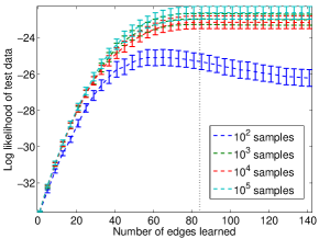
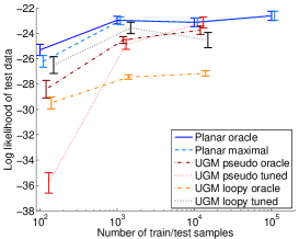
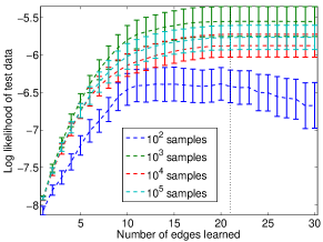
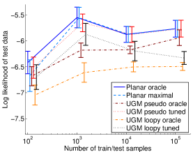
We present the results of experiments evaluating our algorithm on known models with simulated data to evaluate the correctness of the learned models. We generate two styles of known Ising models: a $7\times 7$ grid ($n=49$) with zero-field; and a $12$-node outer planar model where nodes have non-zero mean; shown in Figures 1(a) and 1(d). The edge parameters are chosen uniformly randomly between $-1$ and $1$ with the condition that the absolute value be greater than a threshold (chosen to be $0.05$) so as to avoid edges with negligible interactions. We use Gibbs sampling to obtain samples from this model and calculate empirical moments from these samples which are then passed as input to our algorithm. We run 10 trials of randomly generated edge parameters and data samples. Though our algorithm can run on graphs with many more nodes, we choose small examples here to illustrate the result effectively. On the outer planar model, we ensure that the first moments of all the nodes are satisfied by starting our algorithm with the auxiliary node connected to all other nodes.

As the planar learning algorithm adds edges to the model, the likelihood of the training data is guaranteed to increase. We assess how adding edges affects the likelihood of out-of-sample test data. Figures 1(b) and 1(e) demonstrate that likelihood on test sets generally increases as edges are added up to the maximal planar graph. The true number of edges in each synthetic graph is marked with a vertical dotted line. On the smallest datasets ($100$ samples) the out-of-sample performance begins to degrade, a sign of over-fitting the training data; yet the likelihood of the maximal graph is not significantly worse than the best likelihood obtained (with fewer edges).

We also compare against a Markov random field (MRF) learning algorithm for binary data (Schmidt et al., 2008), as implemented in the undirected graphical model learning Matlab package, UGMLearn. UGM is not restricted to learning planar graphs. The objective is optimized via projected gradient descent. We try two versions of the objective function, one using pseudo-likelihood and the other using loopy belief propagation for inference. UGM employs a regularization parameter which we set using two different methods. First, we used the tuning method on validation data as detailed in Schmidt et al. (2008). That is, we split the data into two parts, train on half the data using 7 different values for the parameter, measure the data likelihood of the other half of the data and vice-versa, then select the parameter value that maximizes the validation data likelihood across both folds. The learned model is trained on the full training data with the tuned regularization parameter value. The second method for setting the regularization parameter we call the oracle method, where we select the learned model at the true number of edges, $k$, in our known models. For UGM, we set the regularization parameter via linear search until $k$ edges are learned.

We compare the likelihood of test data from the various learned models in Figures 1(c) and 1(f). For comparison, we selected the maximal planar graph that our algorithm learns, Planar maximal; as well as the planar graph learned if the algorithm were stopped when the true number of edges are learned, Planar oracle. We compare against UGM pseudo tuned and UGM loopy tuned, both of which tune the regularization parameter on validation data; but the former uses pseudo-likelihood in learning and the latter uses loopy belief propagation. The tuning method is the most common way of selecting the regularization parameter, but tends to produce relatively dense graphs. For fair comparison, we also show the likelihood of UGM pseudo oracle and UGM loopy oracle; that is, the model with the known true number of edges.

Figures 1(c) and 1(f) show that our greedy planar Ising model learning algorithm is at least as accurate and often better than the UGM learning algorithms on these inputs. As mentioned earlier, we see that Planar maximal and Planar oracle fit test data nearly equally well. On the outer planar model, UGM pseudo tuned performs nearly as well as our planar algorithm, yet on the larger grid model it performs quite poorly at the smaller sample sizes. UGM loopy tuned performs more consistently close to our planar algorithm, but it seems that loopy belief propagation performs worse at large sample sizes.

On the largest dataset ($10^{5}$ samples) of the $7\times 7$ grid model, UGM was aborted after running for 40 hours without reaching convergence on a single run, and so results are not available.

5 Application: Modeling Correlations of Senator Voting

(a) Learned planar graphical model representing the senator voting pattern

(b) Comparison of algorithms

Figure 2: Senator voting results. (a) Blue nodes represent Democrats, red nodes represent Republicans and black nodes represents Independents. We use a force-directed graph drawing algorithm (Fruchterman and Reingold, 1991). (b) Likelihood of holdout data versus the number of edges in the learned graph. Note the break in the x-axis, due to tuned UGM learning dense graphs. On the tuned UGM models, we indicate standard error on number of edges learned.

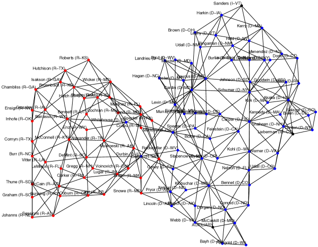
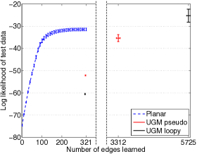
We consider an interesting application of our algorithm to model correlations of senator voting following Banerjee et al. (2008). We use senator voting data from the years 2009 and 2010 to calculate correlations in the voting patterns among senators. A Yea vote is treated as $+1$ and a Nay vote is treated as $-1$. We also treat non-votes as $-1$, but only consider senators who voted in at least $\frac{3}{4}$ of the votes to limit bias. The data includes $n=108$ variables and 645 samples. To accommodate the non-zero mean data we add an auxiliary node and allow the algorithm to select the connections between it and other nodes. We run a 10-fold cross-validation, training on 90% of the data and measuring likelihood on the held-out 10% of data. Figure 2(b) shows that the likelihood of test data increases as edges are added. We also show the likelihood of cross-validation test data for the UGM pseudo and UGM loopy algorithms for two different methods of choosing the value of the regularization parameter: (1) the value that produces the same number of edges as the maximal planar graph (at 318 edges); and (2) the value selected by tuning with validation data (at a variable number of edges, typically a dense graph). The likelihood of the sparse UGM models are significantly worse than the planar model. Only the UGM loopy algorithm at a very dense (nearly fully connected) graph has better fit to test data.

The maximal planar graph learned from the full dataset, shown in Figure 2, conveys many facts that are already known to us. For instance, the graph shows Sanders with edges only to Democrats which makes sense because he caucuses with Democrats. Same is the case with Lieberman. The graph also shows the senate minority leader McConnell well connected to other Republicans though the same is not true of the senate majority leader Reid. The learned UGM models can be seen in the Supplement, and they show that the non-planar models are qualitatively different, learning one or two densely connected components.

6 Conclusion and Future Work

We provide a greedy heuristic to obtain the maximum-likelihood planar Ising model approximation to a collection of binary random variables with known pairwise marginals. The algorithm is simple to implement with the help of known methods for tractable exact inference in planar Ising models, efficient methods for planarity testing and embedding of planar graphs. Empirical results of our algorithm on sample data and on the senate voting record show that it is competitive with arbitrary (non-planar) graph learning.

Many directions for further work are suggested by the methods and results of this paper. Firstly, we know that the greedy algorithm is not guaranteed to find the best planar graph. In the Supplement, we provide an enlightening counterexample in which the combination of the planarity restriction and greedy method prevent the correct model from being learned. That counterexample suggests strategies one might consider to further refine the estimate. One strategy would be to allow the greedy algorithm to prune edges which turn out to be less important once later edges are added. It would also be feasible to implement a multi-step greedy look-ahead search technique for selection of which edge to add (or prune) next.

Another limitation is that our current framework only allows learning planar graphical models on the set of observed random variables and requires that all variables are observed in each sample. One could imagine extensions of our approach to handle missing samples or to try to identify hidden variables that were not seen in the data. This concept offers another avenue to achieve a better fit to data that is not well-approximated by a planar graph among just the set of observed nodes, but might be well-approximated as the marginal distribution of a planar model with more nodes.

Supplementary Appendix

Appendix A Proofs

Proposition $1$.

Let the probability distributions corresponding to $G$ and $\widehat{G}$ be $P$ and $\widehat{P}$ respectively and the corresponding expectations be $\mathbb{E}$ and $\widehat{\mathbb{E}}$ respectively. For the partition function, we have that

$$\begin{array}[]{rl}\widehat{Z}&=\displaystyle\sum_{x_{\widehat{V}}}\exp\left(\displaystyle\sum_{\{i,j\}\in\widehat{E}}\widehat{\theta}_{ij}x_{i}x_{j}\right)\\ &=\displaystyle\sum_{x_{\widehat{V}}}\exp\left(x_{n+1}\displaystyle\sum_{i\in V}\theta_{i}x_{i}+\displaystyle\sum_{\{i,j\}\in E}\theta_{ij}x_{i}x_{j}\right)\\ &=\displaystyle\sum_{x_{V}}\exp\left(\displaystyle\sum_{i\in V}\theta_{i}x_{i}+\displaystyle\sum_{\{i,j\}\in E}\theta_{ij}x_{i}x_{j}\right)\\ &\;\;+\displaystyle\sum_{x_{V}}\exp\left(-\displaystyle\sum_{i\in V}\theta_{i}x_{i}+\displaystyle\sum_{\{i,j\}\in E}\theta_{ij}x_{i}x_{j}\right)\\ &=2\displaystyle\sum_{x_{V}}\exp\left(\displaystyle\sum_{i\in V}\theta_{i}x_{i}+\displaystyle\sum_{\{i,j\}\in E}\theta_{ij}x_{i}x_{j}\right)\\ &=2Z\end{array}$$

where the fourth equality follows from the symmetry between $-1$ and $1$ in an Ising model.

For the second part, since $\widehat{P}$ is zero-field, we have that

$$\widehat{\mathbb{E}}[x_{i}]=0\;\forall\;i\in\widehat{V}$$

Now consider any $\{i,j\}\in E$. If $x_{n+1}$ is fixed to a value of $1$, then the model is the same as original on $V$ and we have

$$\widehat{\mathbb{E}}[x_{i}x_{j}\mid x_{n+1}=1]=\mathbb{E}[x_{i}x_{j}]\;\forall\;\{i,j\}\in E$$

By symmetry (between $-1$ and $1$) in the model, the same is true for $x_{n+1}=-1$ and so we have

$$\begin{array}[]{rl}&\widehat{\mathbb{E}}[x_{i}x_{j}]\\ &=\widehat{\mathbb{E}}[x_{i}x_{j}\mid x_{n+1}=1]\widehat{P}(x_{n+1}=1)\\ &\;+\widehat{\mathbb{E}}[x_{i}x_{j}\mid x_{n+1}=-1]\widehat{P}(x_{n+1}=-1)\\ &=\mathbb{E}[x_{i}x_{j}]\end{array}$$

Fixing $x_{n+1}$ to a value of $1$, we have

$$\widehat{\mathbb{E}}[x_{i}\mid x_{n+1}=1]=\mathbb{E}[x_{i}]\;\forall\;i\in V$$

and by symmetry

$$\widehat{\mathbb{E}}[x_{i}\mid x_{n+1}=-1]=-\mathbb{E}[x_{i}]\;\forall\;i\in V$$

Combining the two equations above, we have

$$\begin{array}[]{rl}&\widehat{\mathbb{E}}[x_{i}x_{n+1}]\\ &=\widehat{\mathbb{E}}[x_{i}\mid x_{n+1}=1]\widehat{P}(x_{n+1}=1)\\ &\;+\widehat{\mathbb{E}}[-x_{i}\mid x_{n+1}=-1]\widehat{P}(x_{n+1}=-1)\\ &=\mathbb{E}[x_{i}]\end{array}$$

∎

Proposition $2$.

From Theorem $1$, we see that the log partition function can be written as

$$\Phi(\theta)=n\log 2+\displaystyle\sum_{\{i,j\}\in E}\log\cosh\theta_{ij}+\frac{1}{2}\log\det(I-AD)$$

where $A$ and $D$ are as given in Theorem $1$. For the derivatives, we have

$$\begin{array}[]{rl}\frac{\partial\Phi(\theta)}{\partial\theta_{ij}}&=\tanh\theta_{ij}+\frac{1}{2}\mbox{Tr}\left((I-AD)^{-1}\frac{\partial(I-AD)}{\partial\theta_{ij}}\right)\\ &=\tanh\theta_{ij}-\frac{1}{2}\mbox{Tr}\left((I-AD)^{-1}AD^{\prime}_{ij}\right)\\ &=w_{ij}-\frac{1}{2}(1-w_{ij})^{2}\left(S_{ij,ij}+S_{ji,ji}\right)\end{array}$$

where $D^{\prime}_{ij}$ is the derivative of the matrix $D$ with respect to $\theta_{ij}$. The first equality follows from chain rule and the fact that $\nabla K=K^{-1}$ for any matrix $K$. Please refer to Boyd and Vandenberghe (2004) for details.

For the Hessian, we have

$$\begin{array}[]{rl}\frac{\partial^{2}\Phi(\theta)}{\partial\theta_{ij}^{2}}&=\frac{1}{Z(\theta)}\frac{\partial^{2}Z(\theta)}{\partial\theta_{ij}^{2}}-\frac{1}{Z(\theta)^{2}}\left(\frac{\partial Z(\theta)}{\partial\theta_{ij}}\right)^{2}\\ &=1-\mu_{ij}^{2}\end{array}$$

For $\{i,j\}\neq\{k,l\}$, following Boyd and Vandenberghe (2004), we have

$$\begin{array}[]{rl}\frac{\partial^{2}\Phi(\theta)}{\partial\theta_{ij}\partial\theta_{kl}}&=-\frac{1}{2}\mbox{Tr}\left(SD^{\prime}_{ij}SD^{\prime}_{kl}\right)\\ &=-\frac{1}{2}(1-w_{ij}^{2})\left(S_{ij,kl}S_{kl,ij}+S_{ji,kl}S_{kl,ji}\right.\\ &\;\;\;\;\left.+S_{ij,lk}S_{lk,ij}+S_{ji,lk}S_{lk,ji}\right)(1-w_{kl}^{2})\end{array}$$

On the other hand, we also have

$$\begin{array}[]{rl}T_{ij,kl}&=e_{ij}^{T}(I+P)(S\circ S^{T})(I+P)e_{kl}\\ &=(e_{ij}+e_{ji})^{T}(S\circ S^{T})(e_{kl}+e_{lk})\\ &=(S\circ S^{T})_{ij,kl}+(S\circ S^{T})_{ij,lk}\\ &\;\;\;+(S\circ S^{T})_{ji,kl}+(S\circ S^{T})_{ji,lk}\\ &=S_{ij,kl}S_{kl,ij}+S_{ji,kl}S_{kl,ji}\\ &\;\;\;+S_{ij,lk}S_{lk,ij}+S_{ji,lk}S_{lk,ji}\end{array}$$

where $e_{ij}$ is the unit vector with $1$ in the $ij^{\mbox{th}}$ position and $0$ everywhere else. Using the above two equations, we obtain

$$H_{ij,kl}=-\frac{1}{2}(1-w_{ij}^{2})T_{ij,kl}(1-w_{kl}^{2})$$

∎

Proposition $4$.

The proof follows from the following steps of inequalities.

$$\begin{array}[]{rl}D(P,P_{G})&=D(P,P_{G+ij})+D(P_{G+ij},P_{G})\\ &=D(P,P_{G+ij})+\\ &\;\;\;D(P_{G+ij}(x_{i},x_{j}),P_{G}(x_{i},x_{j}))+\\ &\;\;\;D(P_{G+ij}(x_{V-ij}),P_{G}(x_{V-ij}))\\ &\geq D(P,P_{G+ij})+\\ &\;\;\;D(P_{G+ij}(x_{i},x_{j}),P_{G}(x_{i},x_{j}))+\\ &\geq D(P,P_{G+ij})+\\ &\;\;\;D(P(x_{i},x_{j}),P_{G}(x_{i},x_{j}))\end{array}$$

where the first step follows from the Pythagorean law of information projection (Amari et al., 1992), the second step follows from the conditional rule of relative entropy (Cover and Thomas, 2006), the third step follows from the information inequality (Cover and Thomas, 2006) and finally the fourth step follows from the property of information projection to $G+ij$ (Wainwright and Jordan, 2008). ∎

Appendix B Experiments: Counter Example

The result presented in Figure 3 illustrates the fact that our algorithm does not always recover the exact structure even when the underlying graph is planar and the algorithm is given exact moments as inputs. This counterexample gives insight into how the greedy algorithm works. The basic idea is that graphical models can have nodes which are not neighbors but are more correlated than some other nodes which are neighbors. If the spurious edges corresponding to these highly correlated nodes are added early on in the algorithm, then the actual edges may have to be left out because of the planarity restriction.

(a) Counter example original

(b) Recovered model

Figure 3: Example graphical models. (a) Counter example. (b) The recovered graphical model has one spurious edge $\{a,e\}$ and one missing edge $\{c,d\}$.

We define a zero-field Ising model on the graph in Figure 3(a) with the edge parameters as follows: $\theta_{bc}=\theta_{cd}=\theta_{bd}=0.1$ and $\theta_{ij}=1$ for all the other edges. Figure 3(a) shows the edge parameters in the graph pictorially using the intensity of the edges - higher the intensity of an edge, higher the corresponding edge parameter. With these edge parameters, the correlation between nodes $a$ and $e$ is greater than the correlation between any other pair of nodes. This leads to the edge between $a$ and $e$ to be the first edge added in the algorithm. However, since $K5$ (the complete graph on $5$ nodes) is not planar, one of the actual edges is missed in the output graph as shown in Figure 3(b).

Appendix C Example Application: UGM Learned Models

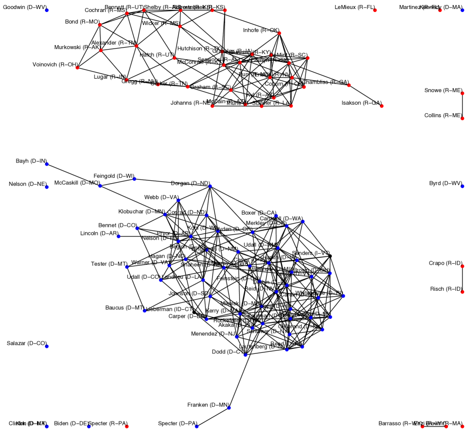
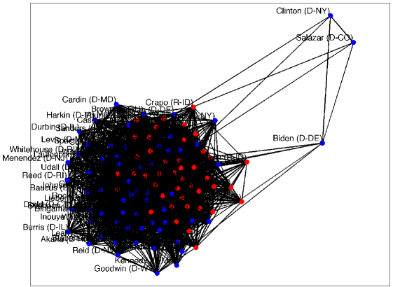
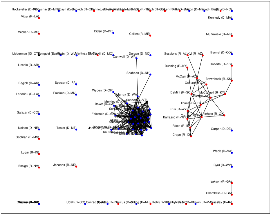
For comparison to our planar learning algorithm, we provide the results of using the UGM MRF learning algorithm on the senate voting data. For all figures, we use a force-directed graph drawing algorithm (Fruchterman and Reingold, 1991). Figure 4 presents the graph learned using pseudolikelihood, UGM pseudo, from the full dataset with the regularization parameter set to obtain the same number of edges as learned in the planar case (318 edges). Figure 5 presents the graph learned using pseudolikelihood, UGM pseudo tuned, from the full dataset after selecting the regularization parameter from cross-validation tuning. Figure 6 presents the graph learned using loopy belief propagation, UGM loopy, from the full dataset with the regularization parameter set to obtain 318 edges. The graph learned using UGM loopy tuned is not displayed because it is a nearly fully-connected graph providing no visual information.

Figure 4: Senate voting graph learned by UGM pseudo with 318 edges. Blue nodes represent Democrats, red nodes represent Republicans and black nodes represent Independents.

Figure 5: Senate voting graph learned by UGM pseudo tuned. Blue nodes represent Democrats, red nodes represent Republicans and black nodes represent Independents.

Figure 6: Senate voting graph learned by UGM loopy with 318 edges. Blue nodes represent Democrats, red nodes represent Republicans and black nodes represent Independents.

References

- Abbeel et al. (2006) P. Abbeel, D. Koller, and A. Ng. Learning factor graphs in polynomial time and sample complexity. J. Mach. Learn. Res., 7, 2006.
- Akaike (1974) H. Akaike. A new look at the statistical model identification. IEEE Trans. Automatic Control, 19(6), 1974.
- Amari et al. (1992) S. Amari, K. Kurata, and H. Nagaoka. Information geometry of Boltzmann machines. IEEE Trans. Neural Networks, 3(2), 1992.
- Bach and Jordan (2001) F. Bach and M. Jordan. Thin junction trees. In NIPS, 2001.
- Banerjee et al. (2008) O. Banerjee, L. El Ghaoui, and A. d’Aspremont. Model selection through sparse maximum likelihood estimation for multivariate Gaussian or binary data. J. Mach. Learn. Res., 9, 2008.
- Barndorff-Nielsen (1979) O. Barndorff-Nielsen. Information and exponential families in statistical theory. Bull. Amer. Math. Soc., 1979.
- Boyd and Vandenberghe (2004) S. Boyd and L. Vandenberghe. Convex Optimization. Cambridge U. Press, 2004.
- Chow and Liu (1968) C. Chow and C. Liu. Approximating discrete probability distributions with dependence trees. IEEE Trans. on Information Theory, 14, 1968.
- Chrobak and Payne (1995) M. Chrobak and T. Payne. A linear-time algorithm for drawing a planar graph on a grid. Infor. Processing Letters, 54(4), 1995.
- Cover and Thomas (2006) T. Cover and J. Thomas. Elements of Information Theory (Wiley Series in Telecommunications and Signal Processing). Wiley-Interscience, 2006.
- Deshpande et al. (2001) A. Deshpande, M. Garofalakis, and M. Jordan. Efficient stepwise selection in decomposable models. In UAI, 2001.
- Fisher (1966) M. Fisher. On the dimer solution of planar Ising models. J. Math. Phys., 7(10), 1966.
- Fruchterman and Reingold (1991) T. Fruchterman and E. Reingold. Graph drawing by force-directed placement. Software: Practice and Experience, 21(11):1129–1164, 1991.
- Galluccio et al. (2000) A. Galluccio, M. Loebl, and J. Vondrak. New algorithm for the Ising problem: Partition function for finite lattice graphs. Physical Review Letters, 84(26), 2000.
- Globerson and Jaakkola (2007) A. Globerson and T. Jaakkola. Approximate inference using planar graph decomposition. In NIPS, 2007.
- Kac and Ward (1952) M. Kac and J. Ward. A combinatorial solution of the two-dimensional Ising model. Phys. Rev., 88(6), 1952.
- Karger and Srebro (2001) D. Karger and N. Srebro. Learning Markov networks: Maximum bounded tree-width graphs. In SODA, 2001.
- Kasteleyn (1963) P. Kasteleyn. Dimer statistics and phase transitions. J. Math. Phys., 4(2), 1963.
- Lauritzen (1996) S. Lauritzen. Graphical Models. Oxford U. Press, 1996.
- Lee et al. (2006) S. Lee, V. Ganapathi, and D. Koller. Efficient structure learning of Markov networks using l1-regularization. In NIPS, 2006.
- Lipton and Tarjan (1979) R. Lipton and R. Tarjan. A separator theorem for planar graphs. SIAM J. Applied Math., 36(2), 1979.
- Lipton et al. (1979) R. Lipton, D. Rose, and R. Tarjan. Generalized nested dissection. SIAM J. Numer. Analysis, 16(2), 1979.
- Loebl (2010) M. Loebl. Discrete Mathematics in Statistical Physics. Vieweg + Teubner, 2010.
- MacKay (2003) D. MacKay. Information Theory, Inference and Learning Algorithms. Cambridge U. Press, 2003.
- Onsager (1944) L. Onsager. Crystal statistics. i. a two-dimensional model with an order-disorder transition. Phys. Rev., 65(3-4), 1944.
- Ravikumar et al. (2010) P. Ravikumar, M. Wainwright, and J. Lafferty. High-dimensional graphical model selection using -regularized logistic regression. Annals of Statistics, 38(3), 2010.
- Schmidt et al. (2008) M. Schmidt, K. Murphy, G. Fung, and R. Rosales. Structure learning in random fields for heart motion abnormality detection. In Computer Vision and Pattern Recognition (CVPR), 2008 IEEE Conference on, 2008.
- Schraudolph and Kamenetsky (2008) N. Schraudolph and D. Kamenetsky. Efficient exact inference in planar Ising models. In NIPS, 2008.
- Schwarz (1978) G. Schwarz. Estimating the dimension of a model. Annals of Stat., 6(2), 1978.
- Shahaf et al. (2009) D. Shahaf, A. Checketka, and C. Guestrin. Learning thin junction trees via graph cuts. In AISTATS, 2009.
- Sherman (1960) S. Sherman. Combinatorial aspects of the Ising model for ferromagnetism. i. a conjecture of Feynman on paths and graphs. J. Math. Phys., 1(3), 1960.
- Wainwright and Jordan (2008) M. Wainwright and M. Jordan. Graphical Models, Exponential Families, and Variational Inference. Now Publishers Inc., 2008.
- Zhang (1993) P. Zhang. Model selection via multifold cross validation. Annals of Stat., 21(1), 1993.