EXIT-Chart Aided Near-Capacity
Quantum Turbo Code Design

Abstract

High detection complexity is the main impediment in future Gigabit-wireless systems. However, a quantum-based detector is capable of simultaneously detecting hundreds of user signals by virtue of its inherent parallel nature. This in turn requires near-capacity quantum error correction codes for protecting the constituent qubits of the quantum detector against the undesirable environmental decoherence. In this quest, we appropriately adapt the conventional non-binary EXtrinsic Information Transfer (EXIT) charts for quantum turbo codes by exploiting the intrinsic quantum-to-classical isomorphism. The EXIT chart analysis not only allows us to dispense with the time-consuming Monte-Carlo simulations, but also facilitates the design of near-capacity codes without resorting to the analysis of their distance spectra. We have demonstrated that our EXIT chart predictions are in line with the Monte-Carlo simulations results. We have also optimized the entanglement-assisted QTC using EXIT charts, which outperforms the existing distance spectra based QTCs. More explicitly, the performance of our optimized QTC is as close as $0.3$ dB to the corresponding hashing bound.

I Introduction

Multi-User Multiple-Input Multiple-Output (MU-MIMO) [1, 2] and massive MIMO [3] schemes are promising candidates for the future generation Gigabit-wireless system. However, the corresponding detection complexity increases exponentially with the number of users and antennas, when aiming for approaching the optimum Maximum-Likelihood (ML) performance. An attractive solution to this exponentially escalating complexity problem is to perform the ML detection in the quantum domain, since quantum computing allows parallel evaluations of a function at a complexity cost that is equivalent to a single classical evaluation [4, 5]. However, a quantum detector requires powerful Quantum Error Correction codes (QECC’s) for stabilizing and protecting the fragile constituent quantum bits (qubits) against the undesirable quantum decoherence, when they interact with the environment [4, 6]. Furthermore, quantum-based wireless transmission is capable of supporting secure data dissemination [4, 7], where any ‘measurement’ or ‘observation’ by an eavesdropper will destroy the quantum entanglement, hence intimating the parties concerned [4]. However, this requires powerful QECC’s for the reliable transmission of qubits across the wireless communication channels. Hence, near-capacity QECC’s are the vital enabling technique for future generations of wireless systems, which are both reliable and secure, yet operate at an affordable detection complexity.

Classical turbo codes operate almost arbitrarily close to the Shannon limit, which inspired researchers to achieve a comparable near-capacity performance for quantum systems [8, 9, 10, 11, 12]. In this quest, Poulin et al. developed the theory of Quantum Turbo Codes (QTCs) in [8, 9], based on the interleaved serial concatenation of Quantum Convolutional Codes (QCCs) [13, 14, 15, 16], and investigated their behaviour on a quantum depolarizing channel. It was found in [8, 17] that the constituent QCCs cannot be simultaneously recursive and non-catastrophic. Since recursive nature of the inner code is essential for ensuring an unbounded minimum distance, while the non-catastrophic nature is required for achieving decoding convergence, the QTCs of [8, 9] had a bounded minimum distance. More explicitly, the design of Poulin et al. [8, 9] was based on non-recursive and non-catastrophic convolutional codes. Later, Wilde and Hseih [10] extended the concept of pre-shared entanglement to QTCs, which facilitated the design of QTCs having an unbounded minimum distance. Wilde et al. also introduced the notion of extrinsic information to the iterative decoding of QTCs and investigated various code structures in [11].

The search for the optimal components of a QTC has been so far confined to the analysis of the constituent QCC distance spectra, followed by intensive Monte-Carlo simulations for determining the convergence threshold of the resultant QTC, as detailed in [9, 11]. While the distance spectrum dominates a turbo code’s performance in the Bit Error Rate (BER) floor region, it has a relatively insignificant impact on the convergence properties in the turbo-cliff region [18]. Therefore, having a good distance spectrum does not guarantee having a near-capacity performance - in fact, often there is a trade-off between them. To circumvent this problem and to dispense with time-consuming Monte-Carlo simulations, in this contribution we extend the application of EXIT charts to the design of quantum turbo codes.

More explicitly,

• We have appropriately adapted the conventional non-binary EXIT chart based design approach to the family of quantum turbo codes based on the underlying quantum-to-classical isomorphism. Similar to the classical codes, our EXIT chart predictions are in line with the Monte-Carlo simulation results.

• We have analyzed the behaviour of both an un-assisted (non-recursive) and of an entanglement-assisted (recursive) inner convolutional code using EXIT charts for demonstrating that, similar to their classical counterparts, recursive inner quantum codes constitute families of QTCs having an unbounded minimum distance.

• For the sake of approaching the achievable capacity, we have optimized the constituent inner and outer components of QTC using EXIT charts. In contrast to the distance spectra based QTCs of [11] whose performance is within $0.9$ dB of the hashing bound, our optimized QTC operates within $0.3$ dB of the capacity limit. However, our intention was not to carry out an exhaustive code search over the potentially excessive parameter-space, but instead to demonstrate how our EXIT-chart based approach may be involved for quantum codes. This new design-approach is expected to stimulate further interest in the EXIT-chart based near-capacity design of various concatenated quantum codes.

This paper is organized as follows. Section II provides a rudimentary introduction to quantum stabilizer codes and QTCs. We will then present our proposed EXIT-chart based approach conceived for quantum turbo codes in Section III. Our results will be discussed in Section IV, while our conclusions are offered in Section V.

II Preliminaries

The constituent convolutional codes of a QTC belong to the class of stabilizer codes [19], which are analogous to classical linear block codes. We will here briefly review the basics of stabilizer codes in order to highlight this relationship for the benefit of readers with background in classical channel coding. This will be followed by a brief discussion of QTCs.

II-A Stabilizer Codes

Qubits collapse to classical bits upon measurement [6, 5]. This prevents us from directly applying classical error correction techniques for reliable quantum transmission. Quantum error correction codes circumvent this problem by observing the error syndromes without reading the actual quantum information. Hence, quantum stabilizer codes invoke the syndrome decoding approach of classical linear block codes for estimating the errors incurred during transmission.

Let us first recall some basic definitions [6].

Pauli Operators

The $\mathbf{I}$, $\mathbf{X}$, $\mathbf{Y}$ and $\mathbf{Z}$ Pauli operators are defined by the following matrices:

$$\mathbf{I} =\begin{pmatrix}1&0\\ 0&1\end{pmatrix},\ \mathbf{X}=\begin{pmatrix}0&1\\ 1&0\end{pmatrix},$$

$$\mathbf{Y} =\begin{pmatrix}0&-i\\ i&0\end{pmatrix},\ \mathbf{Z}=\begin{pmatrix}1&0\\ 0&-1\end{pmatrix},$$ (1)

where the $\mathbf{X}$, $\mathbf{Y}$ and $\mathbf{Z}$ operators anti-commute with each other.

Pauli Group

A single qubit Pauli group $\mathcal{G}_{1}$ consists of all the Pauli matrices of Eq. (1) together with the multiplicative factors $\pm 1$ and $\pm i$, i.e. we have:

$$\mathcal{G}_{1}\equiv\{\pm\mathbf{I},\pm i\mathbf{I},\pm\mathbf{X},\pm i\mathbf{X},\pm\mathbf{Y},\pm i\mathbf{Y},\pm\mathbf{Z},\pm i\mathbf{Z}\}.$$ (2)

The general Pauli group $\mathcal{G}_{n}$ is an $n$-fold tensor product of $\mathcal{G}_{1}$.

Depolarizing Channel

The depolarizing channel characterized by the probability $p$ inflicts an $n$-tuple error $\mathcal{P}\in\mathcal{G}_{n}$ on $n$ qubits, where the $i^{th}$ qubit may experience either a bit flip ($\mathbf{X}$), a phase flip ($\mathbf{Z}$) or both ($\mathbf{Y}$) with a probability of $p/3$.

An $[n,k]$ Quantum Stabilizer Code (QSC), constructed over a code space $\mathcal{C}$, is defined by a set of $(n-k)$ independent commuting $n$-tuple Pauli operators $g_{i}$, for $1\leq i\leq(n-k)$. The corresponding encoder then maps the information word (logical qubits) $|\psi\rangle\in\mathbb{C}^{2^{k}}$ onto the codeword (physical qubits) $|\overline{\psi}\rangle\in\mathbb{C}^{2^{n}}$, where $\mathbb{C}^{d}$ denotes the $d$-dimensional Hilbert space. More specifically, the corresponding stabilizer group $\mathcal{H}$ contains both $g_{i}$ and all the products of $g_{i}$ for $1\leq i\leq(n-k)$ and forms an abelian subgroup of $\mathcal{G}_{n}$. A unique feature of these operators is that they do not change the state of valid codewords, while yielding an eigenvalue of $-1$ for corrupted states. Consequently, the eigenvalue is $-1$ if the $n$-tuple Pauli error $\mathcal{P}$ anti-commutes with the stabilizer $g_{i}$ and it is $+1$ if $\mathcal{P}$ commutes with $g_{i}$. More explicitly, we have:

$$g_{i}|\hat{\psi}\rangle=\left\{\begin{array}[]{l l}|\overline{\psi}\rangle,&g_{i}\mathcal{P}=\mathcal{P}g_{i}\\ -|\overline{\psi}\rangle,&g_{i}\mathcal{P}=-\mathcal{P}g_{i},\\ \end{array}\right.$$ (3)

where $\mathcal{P}$ is an $n$-tuple Pauli error, $|\overline{\psi}\rangle\in\mathcal{C}$ and $|\hat{\psi}\rangle=\mathcal{P}|\overline{\psi}\rangle$ is the received codeword. The resultant $\pm 1$ eigenvalue gives the corresponding error syndrome, which is $0$ for an eigenvalue of $+1$ and $1$ for an eigenvalue of $-1$. It must be mentioned here that Pauli errors which differ only by the stabilizer group have the same impact on all the codewords and therefore can be corrected by the same recovery operations. This gives quantum codes the intrinsic property of degeneracy [20].

As detailed in [21, 22], QSCs may be characterized in terms of an equivalent binary parity check matrix notation satisfying the commutativity constraint of stabilizers. This can be exploited for designing quantum codes with the aid of known classical codes. The $(n-k)$ stabilizers of an $[n,k]$ stabilizer code can be represented as a concatenation of a pair of $(n-k)\times n$ binary matrices $\mathbf{H}_{z}$ and $\mathbf{H}_{x}$, resulting in the binary parity check matrix $\mathbf{H}$ as given below:

$$\mathbf{H}=[\mathbf{H}_{z}|\mathbf{H}_{x}].$$ (4)

More explicitly, each row of $\mathbf{H}$ corresponds to a stabilizer of $\mathcal{H}$, so that the $i^{th}$ column of $\mathbf{H}_{z}$ and $\mathbf{H}_{x}$ corresponds to the $i^{th}$ qubit and a binary $1$ at these locations represents a $\mathbf{Z}$ and $\mathbf{X}$ Pauli operator, respectively, in the corresponding stabilizer. Moreover, the commutativity requirement of stabilizers is transformed into the orthogonality of rows with respect to the symplectic product defined in [22], as follows:

$$\mathbf{H}_{z}\mathbf{H}_{x}^{T}+\mathbf{H}_{x}\mathbf{H}_{z}^{T}=0.$$ (5)

Conversely, two classical linear codes $\mathbf{H}_{z}$ and $\mathbf{H}_{x}$ can be used to construct a quantum stabilizer code $\mathbf{H}$ of Eq. (4) if $\mathbf{H}_{z}$ and $\mathbf{H}_{x}$ meet the symplectic criterion of Eq. (5).

In line with this discussion, a Pauli error operator $\mathcal{P}$ can be represented by the effective error $P$, which is a binary vector of length $2n$. More specifically, $P$ is a concatenation of $n$ bits for $\mathbf{Z}$ errors, followed by another $n$ bits for $\mathbf{X}$ errors and the resultant syndrome is given by the symplectic product of $\mathbf{H}$ and $P$, which is equivalent to $\mathbf{H}[P_{x}:P_{z}]^{T}$. In other words, the Pauli-$\mathbf{X}$ operator is used for correcting $\mathbf{Z}$ errors, while the Pauli-$\mathbf{Z}$ operator is used for correcting $\mathbf{X}$ errors [6]. Thus, the quantum-domain syndrome is equivalent to the classical-domain binary syndrome and a basic quantum-domain decoding procedure is similar to syndrome based decoding of the equivalent classical code [22]. However, due to the degenerate nature of quantum codes, quantum decoding aims for finding the most likely error coset, while the classical syndrome decoding finds the most likely error.

II-B Quantum Turbo Codes

Analogous to classical Serially Concatenated (SC) turbo codes, QTCs are obtained from the interleaved serial concatenation of QCCs, which belong to the class of stabilizer codes. However, it is more convenient to exploit the circuit-based representation of the constituent codes, rather than the conventional parity-check matrix based syndrome decoding [23]. Before proceeding with the decoding algorithm, we will briefly review the circuit-based representation. This discussion is based on [9].

Let us consider an $(n,k)$ classical linear block code constructed over the code space $C$, which maps the information word $c\in\mathbb{F}^{k}_{2}$ onto the corresponding codeword $\overline{c}\in\mathbb{F}^{n}_{2}$. In the circuit-based representation, the code space $C$ is defined as follows:

$$C=\{\overline{c}=(c:0_{n-k})V\},$$ (6)

where $V$ is an $(n\times n)$-element invertible encoding matrix over $\mathbb{F}_{2}$. Similarly, for an $[n,k]$ quantum stabilizer code, the quantum code space $\mathcal{C}$ is defined as:

$$\mathcal{C}=\{|\overline{\psi}\rangle=\mathcal{V}(|\psi\rangle\otimes|0_{n-k}\rangle)\},$$ (7)

where $\mathcal{V}$ is an $n$-qubit Clifford transformation and $|\psi\rangle\in\mathbb{C}^{2^{k}}$. The corresponding binary encoding matrix $V$ is a unique $(2n\times 2n)$-element matrix such that for any $\mathcal{P}\in\mathcal{G}_{n}$ we have [9]:

$$[\mathcal{V}\mathcal{P}\mathcal{V}^{\dagger}]=[\mathcal{P}]V,$$ (8)

where $[\mathcal{P}]=P$ and $[.]$ denotes the effective Pauli group $G_{n}$ such that $[\mathcal{P}]$ differs from $\mathcal{P}$ by a multiplicative constant, i.e. we have $[\mathcal{P}]=\mathcal{P}/\{\pm 1,\pm\textit{i}\}.$ The rows of $V$, denoted as $V_{i}$ for $1\leq i\leq 2n$, are given by $V_{i}=[\mathcal{V}Z_{i}\mathcal{V}^{\dagger}]=[Z_{i}]V$ for $1\leq i\leq n$ and $V_{i}=[\mathcal{V}X_{i}\mathcal{V}^{\dagger}]=[X_{i}]V$ for $n<i\leq 2n$. Here $X_{i}$ and $Z_{i}$ represents the Pauli $\mathbf{X}$ and $\mathbf{Z}$ operators acting on the $i^{th}$ qubit. Furthermore, any codeword in $\mathcal{C}$ is invariant by $\mathcal{V}Z_{i}\mathcal{V}^{\dagger}$, for $k<i\leq n$, which therefore corresponds to the stabilizer generators $g_{i}$ of Eq. (3). More explicitly, the rows $V_{i}$, for $k<i\leq n$, constitute the $(n-k)\times 2n$ parity check matrix $\mathbf{H}$ of Eq. (4), which meets the symplectic criterion of Eq. (5).

At the decoder, the received codeword $|\hat{\psi}\rangle=\mathcal{P}|\overline{\psi}\rangle$ is passed through the inverse encoder $\mathcal{V}^{{\dagger}}$, which yields the corrupted transmitted information word $\mathcal{L}|\psi\rangle$ and the associated syndrome $\mathcal{S}|0_{n-k}\rangle$, formulated as:

$$\mathcal{V}^{{\dagger}}\mathcal{P}|\overline{\psi}\rangle =\mathcal{V}^{{\dagger}}\mathcal{P}\mathcal{V}(|\psi\rangle\otimes|0_{n-k}\rangle)$$

$$=(\mathcal{L}|\psi\rangle)\otimes(\mathcal{S}|0_{n-k}\rangle),$$ (9)

where $\mathcal{L}$ denotes the error imposed on the logical qubits, while $\mathcal{S}$ represents the error inflicted on the remaining $(n-k)$ qubits. This transmission process is summarized in Fig. 1.

Figure 1: Quantum transmission model.

Since stabilizer codes are analogous to linear block codes, syndrome decoding is employed at the receiver to find the most likely error coset $\mathcal{L}$ given the syndrome $\mathcal{S}$. This is efficiently achieved by exploiting the equivalent binary encoding matrix $V$ of Eq. (2), which decomposes the effective $n$-qubit error imposed on the physical qubits $P=[\mathcal{P}]$ into the effective $k$-qubit error inflicted on the logical qubits $L=[\mathcal{L}]$ and the corresponding effective $(n-k)$-qubit syndrome $S=[\mathcal{S}]$, as portrayed in Fig. 2 and mathematically represented below:

$$PV^{-1}=(L:S).$$ (10)

Figure 2: Circuit representation of the inverse encoder $PV^{-1}=(L:S)$.

More explicitly, $P\in G_{n}$, $L\in G_{k}$ and $S\in G_{n-k}$.

For an $[n,k,m]$ QCC, the encoding matrix $V$ is constructed from repeated uses of the seed transformation $U$ shifted by $n$ qubits, as shown in Fig. $6$ of [9]. More specifically, $U$ is the binary equivalent of an $(n+m)$-qubit symplectic matrix. Furthermore, Eq. (10) may be modified as follows [9]:

$$(P_{t}:M_{t})U^{-1}=(M_{t-1}:L_{t}:S_{t}),$$ (11)

where $t$ and $(t-1)$ denotes the current and previous time instants, respectively, while $M$ is the effective $m$-qubit error on the memory states. Furthermore, $2(n-k)$-element binary vector $S$ of Eq. (10) and (11) can be decomposed into two components, yielding $S=S^{x}+S^{z}$, wher $S^{x}$ and $S^{z}$ are the $\mathbf{X}$ and $\mathbf{Z}$ components of the syndrome $S$, respectively. The $(n-k)$-binary error syndrome computed using the parity check matrix $\mathbf{H}$ only reveals $S^{x}$ but not $S^{z}$ [9]. Therefore, those physical errors which only differ in $S^{z}$ do not have to be differentiated, since they correspond to the same logical error $L$ and can be corrected by the same operations. These are the degenerate errors, which only differ by the stabilizer group as discussed in Section II-A. Consequently, a quantum turbo decoding algorithm aims for finding the most likely error coset acting on the logical qubits, i.e. $L$, which satisfies the syndrome $S^{x}$.

Similar to the classical turbo codes, Quantum turbo decoding invokes an iterative decoding algorithm at the receiver for exchanging extrinsic information [11, 25] between the pair of SC Soft-In Soft-Out (SISO) decoders, as shown in Fig. 3. These SISO decoders employ the degenerate decoding approach of [9]. Let $P_{i}$ and $L_{i}$ denote the error imposed on the physical and logical qubits, while $S^{x}_{i}$ represents the syndrome sequence for the $i^{th}$ decoder. Furthermore, $\mathbf{P}^{a}_{i}(.)$, $\mathbf{P}^{e}_{i}(.)$ and $\mathbf{P}^{o}_{i}(.)$ denote the a-priori, extrinsic and a-posteriori probabilities [25] related to the $i^{th}$ decoder. Based on this notation, the turbo decoding process can be summarized as follows:

• The inner SISO decoder uses the channel information $\mathbf{P}_{ch}(P_{1})$, the a-priori information gleaned from the outer decoder $\mathbf{P}_{1}^{a}(L_{1})$ (initialized to be equiprobable for the first iteration) and the syndrome $S^{x}_{1}$ to compute the extrinsic information $\mathbf{P}_{1}^{e}(L_{1})$.

• $\mathbf{P}_{1}^{e}(L_{1})$ is passed through a quantum interleaver $(\pi)$ to yield a-priori information for the outer decoder $\mathbf{P}_{2}^{a}(P_{2})$.

• Based on the a-priori information $\mathbf{P}_{2}^{a}(P_{2})$ and on the syndrome $S^{x}_{2}$, the outer SISO decoder computes both the a-posteriori information $\mathbf{P}_{2}^{o}(L_{2})$ and the extrinsic information $\mathbf{P}_{2}^{e}(P_{2})$.

• $\mathbf{P}_{2}^{e}(P_{2})$ is de-interleaved to obtain $\mathbf{P}_{1}^{a}(L_{1})$, which is fed back to the inner SISO decoder. This iterative procedure continues until convergence is achieved or the maximum affordable number of iterations is reached.

• Finally, a qubit-based MAP decision is made to determine the most likely error coset $L_{2}$.

Figure 3: Schematic of the quantum turbo decoder. $\mathbf{P}^{a}_{i}(.)$, $\mathbf{P}^{e}_{i}(.)$ and $\mathbf{P}^{o}_{i}(.)$ are the a-priori, extrinsic and a-posteriori probabilities related to the $i^{th}$ decoder; $P_{i}$ and $L_{i}$ denote the error on the physical and logical qubits, while $S^{x}_{i}$ represents the syndrome sequence for the $i^{th}$ decoder.

III Application of EXIT Charts to Quantum Turbo Codes

In this section, we will extend the application of EXIT charts to the quantum domain, by appropriately adapting the conventional non-binary EXIT chart generation technique to the circuit-based quantum syndrome decoding approach. Some of the information presented in this section might seem redundant to the experts of classical channel coding theory. However, since EXIT charts are not widely known in the quantum community, this introduction was necessary to make this treatise accessible to quantum researchers.

III-A EXIT Charts

EXIT charts [18, 25, 26] are capable of visualizing the convergence behaviour of iterative decoding schemes by exploiting the input/output relations of the constituent decoders in terms of their average Mutual Information (MI) characteristics. They have been extensively employed for designing near-capacity classical codes [27, 28, 29]. Let us recall that the EXIT chart of a serially concatenated scheme visualizes the exchange of the following four MI terms:

• average a-priori MI of the inner decoder, $I_{A}^{1}$,

• average a-priori MI of the outer decoder, $I_{A}^{2}$,

• average extrinsic MI of the inner decoder, $I_{E}^{1}$, and

• average extrinsic MI of the outer decoder, $I_{E}^{2}$.

More specifically, $I_{A}^{1}$ and $I_{E}^{1}$ constitute the EXIT curve of the inner decoder, while $I_{A}^{2}$ and $I_{E}^{2}$ yield the EXIT curve of the outer decoder. The MI transfer characteristics of both the decoders are plotted in the same graph, with the $x$ and $y$ axes of the outer decoder swapped. The resultant EXIT chart quantifies the improvement in the mutual information as the iterations proceed, which can be viewed as a stair-case-shaped decoding trajectory. Having an open tunnel between the two EXIT curves ensures that the decoding trajectory reaches the $(1,y)$ point of perfect convergence.

III-B Quantum-to-Classical Isomorphism

Before proceeding with the application of EXIT charts for quantum codes, let us elaborate on the quantum-to-classical isomorphism encapsulated in Eq. (4), which forms the basis of our EXIT chart aided approach. As discussed in Section II-A, a Pauli error operator $\mathcal{P}$ experienced by an $N$-qubit frame transmitted over a depolarizing channel can be modeled by an effective error-vector $P$, which is a binary vector of length $2N$. The first $N$ bits of $P$ denote $Z$ errors, while the remaining $N$ bits represent $\mathbf{X}$ errors, as depicted in Fig. 4. More explicitly, an $\mathbf{X}$ error imposed on the $1^{st}$ qubit will yield a $0$ and a $1$ at the $1^{st}$ and $(N+1)^{th}$ index of $P$, respectively. Similarly, a $\mathbf{Z}$ error imposed on the $1^{st}$ qubit will give a $1$ and a $0$ at the $1^{st}$ and $(N+1)^{th}$ index of $P$, respectively, while a $Y$ error on the $1^{st}$ qubit will result in a $1$ at both the $1^{st}$ as well as $(N+1)^{th}$ index of $P$. Since a depolarizing channel characterized by the probability $p$ incurs $\mathbf{X}$, $\mathbf{Y}$ and $\mathbf{Z}$ errors with an equal probability of $p/3$, the effective error-vector $P$ reduces to two Binary Symmetric Channels (BSCs) having a crossover probability of $2p/3$, where we have one channel for the $\mathbf{Z}$ errors and the other for the $\mathbf{X}$ errors. Hence, a quantum depolarizing channel has been considered analogous to a Binary Symmetric Channel (BSC) [22, 30], whose capacity is given by:

$$C_{\text{BSC}}=1-H_{2}(2p/3),$$ (12)

where $H_{2}$ is the binary entropy function. Using Eq. (4), we can readily infer that the code rate $R_{Q}$ of an $[n,k]$ QSC is related to the equivalent classical code rate $R_{C}$ as follows [22, 31]:

$$R_{C}=\frac{1}{2}\left(1+R_{Q}\right).$$ (13)

Consequently, the corresponding quantum capacity is as follows [22, 31]:

$$C^{Q}_{\text{BSC}}=1-H_{2}(2p/3).$$ (14)

Figure 4: Effective error $(P)$ corresponding to the error imposed on an $N$-qubit frame $(\mathcal{P})$.

	$\mathbf{Z}=0$	$\mathbf{Z}=1$
$\mathbf{X}=0$	$1-p$	$p/3$
$\mathbf{X}=1$	$p/3$	$p/3$

TABLE I: Correlation between $\mathbf{X}$ and $\mathbf{Z}$ errors on th $i^{th}$ qubit in terms of the corresponding probability of occurrence.

However, the two BSCs constituting a quantum depolarizing channel are not entirely independent. There is an inherent correlation between the $\mathbf{X}$ and $\mathbf{Z}$ errors [22], which is characterized in Table I. This correlation is taken into account by the turbo decoder of Fig. 3. Alternatively, a quantum depolarization channel can also be considered equivalent to a $4$-ary symmetric channel. More explicitly, the $i^{th}$ and $(N+i)^{th}$ index of $P$ constitute the $4$-ary symbol. The corresponding classical capacity is equivalent to the maximum rate achievable over each half of the $4$-ary symmetric channel, as follows [22, 31]:

$$C_{\text{4-ary}}=\frac{1}{2}[2-H_{2}(p)-p\log_{2}(3)].$$ (15)

Therefore, using Eq. (13) the corresponding quantum capacity can be readily shown to be [22, 31]:

$$C^{Q}_{\text{4-ary}}=1-H_{2}(p)-p\log_{2}(3),$$ (16)

which is known as the hashing bound.

Recall that a quantum code is equivalent to a classical code through Eq. (4). More specifically, as mentioned in Section II-A, the decoding of a quantum code is essentially carried out with the aid of the equivalent classical code by exploiting the additional property of degeneracy. Quantum codes employ syndrome decoding [23], which yields information about the error-sequence rather than the information-sequence or coded qubits, hence avoiding the observation of the latter sequences, which would collapse them back to the classical domain.

Since a depolarizing channel is analogous to the BSC and a QTC has an equivalent classical representation, we employ the EXIT chart technique to design near-capacity QTCs. The major difference between the EXIT charts conceived for the classical and quantum domains is that while the former models the a-priori information concerning the input bits of the inner encoder (and similarly the output bits of the outer encoder), the latter models the a-priori information concerning the corresponding error-sequence, i.e. the error-sequence related to the input qubits of the inner encoder $L_{1}$ (and similarly error-sequence related to the output qubits of the outer encoder $P_{2}$). This will be dealt with further in the next section.

III-C EXIT Charts for Quantum Turbo Codes

Similar to the classical EXIT charts, in our design we assume that the interleaver length is sufficiently high to ensure that [18, 25]:

• the a-priori values are fairly uncorrelated; and

• the a-priori information has a Gaussian distribution.

Figure 5: System model for generating the EXIT chart of the inner decoder.

Fig. 5 shows the system model used for generating the EXIT chart of the inner decoder. Here, a quantum depolarizing channel having a depolarizing probability of $p$ generates the error sequence $P_{1}$, which is passed through the inverse inner encoder $V_{1}^{-1}$. This yields both the error imposed on the logical qubits $L_{1}$ and the syndrome $S^{x}_{1}$ according to Eq. (10). The a-priori channel block then models the a-priori information $\mathbf{P}^{a}_{1}(L_{1})$ such that the average mutual information between the actual error $L_{1}$ and the a-priori probabilities $\mathbf{P}^{a}_{1}(L_{1})$ is given by $I_{A}(L_{1})$ [18, 25, 26]. More explicitly, we have $I_{A}(L_{1})=I[L_{1},\mathbf{P}^{a}_{1}(L_{1})]$, where $I$ denotes the average mutual information function. As discussed in Section III-B, the $i^{th}$ and $(N+i)^{th}$ bits of the effective error vector $L_{1}$ can be visualized as $4$-ary symbols. Consequently, similar to classical non-binary EXIT charts [32, 33], the a-priori information is modeled using an independent Gaussian distribution with a mean of zero and variance of $\sigma_{A}^{2}$, assuming that the $\mathbf{X}$ and $\mathbf{Z}$ errors constituting the $4$-ary symbols are independent. Using the channel information $\mathbf{P}_{ch}(P_{1})$, syndrome $S^{x}_{1}$ and the a-priori information, the inner SISO decoder yields the extrinsic information $\mathbf{P}^{e}_{1}(L_{1})$ based on the classic forward-backward recursive coefficients $\alpha_{t}$ and $\beta_{t}$ as follows[9]:

• For a coded sequence of duration $N$, let $P_{1}=[P_{1,1},P_{1,2},\dots,P_{1,t},\dots,P_{1,N}]$ and $L_{1}=[L_{1,1},L_{1,2},\dots,L_{1,t},\dots,L_{1,N}]$, where $P_{1,t}\in G_{n}$ and $L_{1,t}\in G_{k}$. More explicitly, $P_{1,t}=[P_{1,t}^{1},P_{1,t}^{2},\dots,P_{1,t}^{n}]$ and $L_{1,t}=[L_{1,t}^{1},L_{1,t}^{2},\dots,L_{1,t}^{k}]$. For the ease of clarification, we will ignore the first subscript, which represents the decoder, in the algorithm given below, i.e. we have $P_{1}=P$ and $L_{1}=L$. Similarly, $S_{1}^{x}=S^{x}$.

• Let $U=(U_{P}:U_{M})$, so that $U_{P}$ is the binary matrix formed by the first $2n$ columns of $U$ of Eq. (11), while $U_{M}$ is the binary matrix formed by the last $2m$ columns of $U$. Therefore, we have:

  $$P_{t}=\left(M_{t-1}:L_{t}:S_{t}\right)U_{P}.$$ (17)

  $$M_{t}=\left(M_{t-1}:L_{t}:S_{t}\right)U_{M}.$$ (18)

• Let $\alpha_{t}\left(M_{t}\right)$ be the forward recursive coefficient, which is defined as follows:

  $$\alpha_{t}\left(M_{t}\right) \triangleq\mathbf{P}\left(M_{t}|S^{x}_{\leq t}\right),$$

  $$\propto\sum_{\mu,\lambda,\sigma}\mathbf{P}^{a}\left(L_{t}=\lambda\right)\mathbf{P}_{ch}\left(P_{t}\right)\alpha_{t-1}\left(\mu\right),$$ (19)

  where $\mu\in G_{m}$, $\lambda\in G_{k}$ and $\sigma\in G_{n-k}$, while $\sigma=\sigma_{x}+\sigma_{z}$, having $\sigma_{x}=S^{x}_{t}$. Furthermore, we have $P_{t}=(\mu:\lambda:\sigma)U_{P}$ and $M_{t}=\left(\mu:\lambda:\sigma\right)U_{M}$. The channel information $\mathbf{P}_{ch}\left(P_{t}\right)$ is computed assuming that each qubit is independently transmitted over a quantum depolarizing channel having a depolarizing probability of $p$, whose channel transition probabilities are given by [9]:

  $$\mathbf{P}_{ch}\left(P_{t}^{i}\right)=\left\{\begin{array}[]{l l}1-p,&\text{if }\mathcal{P}_{t}^{i}=\mathbf{I}\\ p/3,&\text{if }\mathcal{P}_{t}^{i}\in\{\mathbf{X},\mathbf{Z},\mathbf{Y}\}.\\ \end{array}\right.$$ (20)

• Let $\beta_{t}\left(M_{t}\right)$ be the backward recursive coefficient, which is defined as follows:

  $$\beta_{t}\left(M_{t}\right)\triangleq\mathbf{P}\left(M_{t}|S^{x}_{>t}\right),$$

  $$\propto\sum_{\lambda,\sigma}\mathbf{P}^{a}\left(L_{t}=\lambda\right)\mathbf{P}_{ch}\left(P_{t+1}\right)\beta_{t+1}\left(M_{t+1}\right),$$ (21)

  where $P_{t+1}=(M_{t}:\lambda:\sigma)U_{P}$ and $M_{t+1}=\left(M_{t}:\lambda:\sigma\right)U_{M}$.

• Finally, we have the a-posteriori probability $\mathbf{P}^{o}(L_{t})$, which is given by:

  $$\mathbf{P}^{o}(L_{t})\triangleq\mathbf{P}(L_{t}|S^{x}),$$

  $$\propto\sum_{\mu,\sigma}\mathbf{P}^{a}(L_{t})\mathbf{P}_{ch}(P_{t})\alpha_{t-1}\left(\mu\right)\beta_{t}\left(M_{t}\right),$$ (22)

  where $P_{t}=(\mu:L_{t}:\sigma)U_{P}$ and $M_{t}=\left(\mu:L_{t}:\sigma\right)U_{M}$.

• Marginalized probabilities $\mathbf{P}^{o}(L^{j}_{t})$ for $j\in\{0,k-1\}$ are then computed from $\mathbf{P}^{o}(L^{j}_{t})$ and the a-priori information is removed in order to yield the extrinsic probabilities[11], i.e we have:

  $$\ln[\mathbf{P}^{e}(L^{j}_{t})]=\ln[\mathbf{P}^{o}(L^{j}_{t})]-\ln[\mathbf{P}^{a}(L^{j}_{t})].$$ (23)

Finally, the extrinsic average mutual information between $L_{1}$ and $\mathbf{P}^{e}_{1}(L_{1})$ is computed, i.e. $I_{E}(L_{1})=I[L_{1},\mathbf{P}^{e}_{1}(L_{1})]$. Since the equivalent classical capacity of a quantum channel is given by the capacity achievable over each half of the $4$-ary symmetric channel as depicted in Eq. (15), $I_{E}(L_{1})$ is the normalized mutual information of the $4$-ary symbols, which can be computed based on [33, 34] as:

$$I_{E}(L_{1})=\frac{1}{2}\left(2+\mbox{E}\left[\sum_{\text{m}=0}^{3}\mathbf{P}^{e}_{1}(L_{1}^{j(\text{m})})\log_{2}\mathbf{P}^{e}_{1}(L_{1}^{j(\text{m})})\right]\right),$$ (24)

where E is the expectation (or time average) operator and $L_{1}^{j(\text{m})}$ is the $4$-ary $\text{m}^{\text{th}}$ hypothetical error imposed on the logical qubits. More explicitly, since error on each qubit is represented by an equivalent pair of classical bits, $L_{1}^{j(\text{m})}$ is a $4$-ary classical symbol with $\text{m}\in\{0,3\}$. The process is repeated for a range of $I_{A}(L_{1})\in[0,1]$ values for obtaining the extrinsic information transfer characteristics at the depolarizing probability $p$. The resultant inner EXIT function $T_{1}$ of the specific inner decoder may be defined as follows:

$$I_{E}(L_{1})=T_{1}[I_{A}(L_{1}),p],$$ (25)

which is dependent on the depolarizing probability $p$ of the quantum channel.

The system model used for generating the EXIT chart of the outer decoder is depicted in Fig. 6. As inferred from the figure, the EXIT curve of the outer decoder is independent of the channel’s output information. The a-priori information is generated by the a-priori channel based on $P_{2}$ (error on the physical qubits of the second decoder) and $I_{A}(P_{2})$, which is the average Mutual Information (MI) between $P_{2}$ and $\mathbf{P}^{a}_{2}(P_{2})$. Furthermore, as for the inner decoder, $P_{2}$ is passed through the inverse outer encoder $V_{2}^{-1}$ to compute $S^{x}_{2}$, which is fed to the outer SISO decoder to yield the extrinsic information $\mathbf{P}^{e}_{2}(P_{2})$. Based on Eq. (19) and (21), this may be formulated as follows [9]:

$$\mathbf{P}^{o}(P_{t})\triangleq\mathbf{P}(P_{t}|S^{x}),$$

$$\propto\sum_{\mu,\lambda,\sigma}\mathbf{P}(P_{t})\mathbf{P}(L_{t}=\lambda)\alpha_{t-1}\left(\mu\right)\beta_{t}\left(M_{t}\right),$$ (26)

where $P_{t}=(\mu:\lambda:\sigma)U_{P}$ and $M_{t}=\left(\mu:\lambda:\sigma\right)U_{M}$. The resultant probabilities are marginalized and the a-priori information is removed similar to Eq. (23). The average MI between $P_{2}$ and $\mathbf{P}^{e}_{2}(P_{2})$ is then calculated using Eq. (24). The resultant EXIT chart is characterized by the following MI transfer function:

$$I_{E}(P_{2})=T_{2}[I_{A}(P_{2})],$$ (27)

where $T_{2}$ is the outer EXIT function, which is dependent on the specific outer decoder, but is independent of the depolarizing probability $p$.

Figure 6: System model for generating the EXIT chart of the outer decoder.

Finally, the MI transfer characteristics of both decoders characterized by Eq. (25) and Eq. (27) are plotted in the same graph, with the $x$ and $y$ axes of the outer decoder swapped.

IV Results and Discussions

IV-A Accuracy of EXIT Chart Predictions

In order to verify the accuracy of our EXIT-chart based approach, we have analyzed the convergence behaviour of a rate-$1/9$ QTC, consisting of two identical rate-$1/3$ QCCs. More specifically, for both the inner and outer decoders, we have used the configuration termed as “PTO1R” in [10, 11], which is a non-catastrophic but quasi-recursive code.

Our first aim was to predict the convergence threshold using EXIT charts, which would otherwise require time-consuming Word Error Rate/Qubit Error Rate (WER/QBER) simulations. Convergence threshold can be determined by finding the maximum depolarizing probability $p$, which yields a marginally open EXIT tunnel between the EXIT curves of the inner and outer decoder; hence, facilitating an infinitesimally low QBER. Fig. 7 shows the EXIT curves for the inner and outer decoders, where the area under the EXIT curve of the inner decoder decreases upon increasing $p$. Eventually, the inner and outer curves crossover, when $p$ is increased to $p=0.13$. More explicitly, increasing $p$ beyond $0.125$, closes the EXIT tunnel. Hence, the convergence threshold is around $p=0.125$.

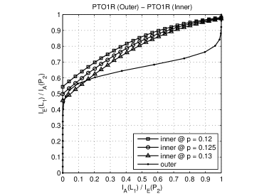
Figure 7: The EXIT curves of a QTC parametrized by the increasing depolarizing probability $p$ (rate-1/9 QTC having PTO1R as both the inner and outer components was used).

Fig. 8 shows two decoding trajectories superimposed on the EXIT chart of Fig. 7 at $p=0.125$. We have used a $30,000$-qubit long interleaver. As seen from Fig. 8, the trajectory successfully reaches the $(x,y)=(1,y)$ point of the EXIT chart. This in turn guarantees an infinitesimally low QBER at $p=0.125$ for an interleaver of infinite length.

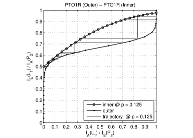
Figure 8: The EXIT chart of a QTC with decoding trajectories at $p=0.125$ (rate-1/9 QTC having PTO1R as both the inner and outer components with an interleaver length of $30,000$ qubits was used).

We have further verified the validity of our EXIT chart predictions using QBER simulations. Fig. 9 shows the QBER performance curve for an interleaver length of $3,000$ qubits. The performance improves upon increasing the number of iterations. More specifically, the turbo-cliff region starts around $p=0.125$, whereby the QBER drops as the iterations proceed. Therefore, our EXIT chart predictions closely follow the Monte-Carlo simulation results.

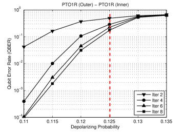
Figure 9: QBER performance curve with increasing iteration number for an interleaver length of 3,000 qubits. Rate-1/9 QTC having PTO1R as both the inner and outer components was used.

IV-B Entanglement-Assisted and Unassisted Inner Codes

All non-catastrophic convolutional codes are non-recursive [9]. Therefore, the resultant families of QTCs have a bounded minimum distance and do not have a true iterative threshold. To circumvent this limitation of QTCs, Wilde et al. [10, 11] proposed to employ entanglement-assisted inner codes, which are recursive as well as non-catastrophic. The resulting families of entanglement-assisted QTCs have an unbounded minimum distance [10, 11], i.e. their minimum distance increases almost linearly with the interleaver length. Here, we verify this by analyzing the inner decoder’s EXIT curves for both the unassisted (non-recursive) and entanglement-assisted (recursive) inner convolutional codes.

For classical recursive inner codes, the inner decoder’s EXIT curve reaches the $(x,y)=(1,1)$ point, which guarantees perfect decoding convergence to a vanishingly low QBER as well as having an unbounded minimum distance for the infinite family of QTCs [9] based on these inner codes. Consequently, the resulting families of QTCs have unbounded minimum distance and hence an arbitrarily low QBER can be achieved for an infinitely long interleaver. This also holds true for recursive quantum convolutional codes, as shown in Fig. 10. In this figure, we compare the inner decoder’s EXIT curves of both the unassisted and the entanglement-assisted QCCs of [10], which are labeled “PTO1R” and “PTO1REA”, respectively. For the PTO1R configuration, decreasing the depolarizing probability from $p=0.14$ to $p=0.12$ shifts the inner decoder’s EXIT curve upwards and towards the $(1,1)$ point. Hence, the EXIT curve will manage to reach the $(1,1)$ point only at very low values of depolarizing probability. By contrast, the EXIT curve of PTO1REA always terminates at $(1,1)$, regardless of the value of $p$. Therefore, provided an open EXIT tunnel exists and the interleaver length is sufficiently long, the decoding trajectories of an entanglement-assisted QTC will always reach the $(1,1)$ point; thus, guaranteeing an arbitrarily low QBER for the infinite family of QTCs based on these inner codes. In other words, the performance improves upon increasing the interleaver length; thus, implying that the minimum distance increases upon increasing the interleaver length and therefore the resultant QTCs have an unbounded minimum distance.

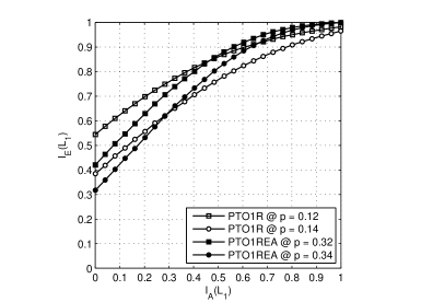
Figure 10: Comparison of the inner EXIT curves of both unassisted and entanglement-assisted QCCs, labeled as PTO1R and PTO1REA respectively.

IV-C Optimized Quantum Turbo Code Design

The QTC design of [10, 11] characterized in Fig. 8 exhibits a large area between the inner and outer decoder’s EXIT curves. The larger the ‘open-tunnel’ area, the farther the QBER performance curve from the achievable capacity limit [25]. Consequently, various distance spectra based QTCs investigated in [11] operate within $0.9$ dB of the hashing bound. For the sake of achieving a near-capacity performance, we minimize the area between the inner and outer EXIT curves, so that a narrow, but still marginally open tunnel exists at the highest possible depolarizing probability. Our aim was to construct a rate-$1/9$ QTC relying on an entanglement-assisted inner code (recursive and non-catastrophic) and an unassisted outer code (non-catastrophic) having a memory of $3$ and a rate of $1/3$. The resultant QTC has an entanglement consumption rate of $6/9$, for which the corresponding maximum tolerable depolarizing probability was shown to be $p_{\max}=0.3779$ in [11].

For the sake of designing a near-capacity QTC operating close to the capacity limit of $p_{\max}=0.3779$, we randomly selected both inner and outer encoders from the Clifford group according to the algorithm of [35] in order to find the inner and outer components, which minimize the area between the corresponding EXIT curves. Based on this design criterion, we found optimal inner and outer code pair whose seed transforms (decimal representation) are given by:

$$U_{\text{inner}}=\{ 4091,3736,2097,1336,1601,279,$$

$$3093,502,1792,3020,226,1100\};$$ (28)

$$U_{\text{outer}}=\{ 1048,3872,3485,2054,983,3164,$$

$$3145,1824,987,3282,2505,1984\}.$$ (29)

Fig. 11 shows the corresponding EXIT chart at the convergence threshold of $p=0.35$. As observed in Fig. 11, a marginally open EXIT tunnel exists between the two curves, which facilitates for the decoding trajectories to reach the $(1,1)$ point. Hence, our optimized QTC has a convergence threshold of $p=0.35$, which is only $\left[10\times\log_{10}(\frac{0.35}{0.3779})\right]=0.3$ dB from the maximum tolerable depolarizing probability of $0.3779$.

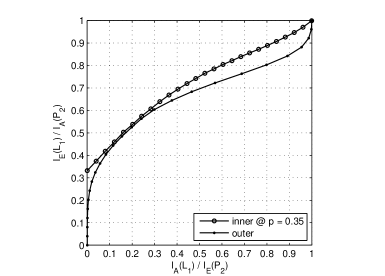
Figure 11: EXIT chart of the optimized rate-$1/9$ QTC (Interleaver length = $30,000$ qubits).

The corresponding QBER performance curves recorded for our optimized design are given in Fig. 12. A maximum of $15$ iterations were used, while the interleaver length was increased from $1500$ to $12,000$. Similar to classical turbo codes, increasing the interleaver length for $p<0.35$ improves the attainable performance.

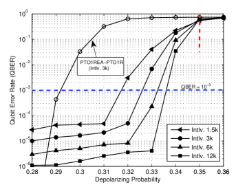
Figure 12: QBER performance curves of the optimized rate-$1/9$ QTC for varying interleaver lengths and a maximum of $15$ iterations.

Furthermore, Fig. 12 also compares our optimized design with the rate-$1/9$ QTC of [11] for an interleaver length of $3000$, which is labeled “PTO1REA-PTO1R” in the figure. For the “PTO1REA-PTO1R” configuration, the turbo cliff region emerges around $0.31$, which is within $0.9$ dB of the capacity limit. Therefore, our EXIT-chart based QTC outperforms the QTC design based on the distance spectrum [11]. More specifically, the “PTO1REA-PTO1R” configuration yields a QBER of $10^{-3}$ at $p=0.2925$, while our optimized QTC gives a QBER of $10^{-3}$ at $p=0.3275$. Hence, our optimized QTC outperforms the ‘PTO1REA-PTO1R” configuration by about $\left[10\times\log_{10}(\frac{0.2925}{0.3275})\right]=0.5$ dB at a QBER of $10^{-3}$. However, our main design objective was to not to carry out an exhaustive code search, but to demonstrate the explicit benefit of our EXIT-chart based approach in the context of quantum codes. It must also be observed in Fig. 12 that a relatively high error floor exists for our optimized design, which is gradually reduced upon increasing the interleaver length. This is because the outer code has a low minimum distance of only $3$. Its truncated distance spectrum is as follows:

$$D(x)= 2x^{3}+19x^{4}+108x^{5}+530x^{6}+2882x^{7}+14179x^{8}+$$

$$62288x^{9}+243234x^{10}+845863x^{11}+1165784x^{12}+$$

$$2501507x^{13}+744394x^{14}.$$

By contrast, the truncated distance spectrum of “PTO1R”, which has a minimum distance of $5$, is given by [11]:

$$D(x)= 11x^{5}+47x^{6}+253x^{7}+1187x^{8}+6024x^{9}+$$

$$30529x^{10}+153051x^{11}+771650x^{12}.$$

Consequently, as gleaned from Fig. 12, the “PTO1REA-PTO1R” configuration has a much lower error floor ($<10^{-6}$), since the outer code “PTO1R” has a higher minimum distance. However, this enlarges the area between the inner and outer decoder’s EXIT curves; thus, driving the performance farther away from the achievable capacity, as depicted in Fig. 8. Hence, there is a trade-off between the minimization of the error floor and achieving a near-capacity performance. More specifically, while the distance-spectrum based design primarily aims for achieving a lower error floor, the EXIT-chart based design strives for achieving a near-capacity performance.

V Conclusions

In this contribution, we have extended the application of classical non-binary EXIT charts to the circuit-based syndrome decoder of quantum turbo codes, in order to facilitate the EXIT-chart based design of QTCs. We have verified the accuracy of our EXIT chart generation approach by comparing the convergence threshold predicted by the EXIT chart to the Monte-Carlo simulation results. Furthermore, we have shown with the aid of EXIT charts that entanglement-assisted recursive QCCs have an unbounded minimum distance. Moreover, we have designed an optimal entanglement-assisted QTC using EXIT charts, which outperforms the distance spectra based QTC of [11] by about $0.5$ dB at a QBER of $10^{-3}$.

References

- [1] S. X. Ng and L. Hanzo, “On the MIMO channel capacity of multidimensional signal sets,” IEEE Transactions on Vehicular Technology, vol. 55, no. 2, pp. 528–536, 2006.
- [2] J.-M. Chung, J. Kim, and D. Han, “Multihop hybrid virtual MIMO scheme for wireless sensor networks,” IEEE Transactions on Vehicular Technology, vol. 61, no. 9, pp. 4069–4078, 2012.
- [3] J. Lee and S.-H. Lee, “A compressed analog feedback strategy for spatially correlated massive MIMO systems,” in IEEE Vehicular Technology Conference (VTC Fall), 2012, pp. 1–6.
- [4] S. Imre and F. Balazs, Quantum Computing and Communications: An Engineering Approach. John Wiley & Sons, 2005.
- [5] P. Botsinis, S. X. Ng, and L. Hanzo, “Quantum search algorithms, quantum wireless, and a low-complexity maximum likelihood iterative quantum multi-user detector design,” IEEE Access, vol. 1, pp. 94–122, 2013. [Online]. Available: http://ieeexplore.ieee.org/xpl/articleDetails.jsp?arnumber=6515077
- [6] M. A. Nielsen and I. L. Chuang, Quantum Computation and Quantum Information. Cambridge University Press, 2000.
- [7] X. Zhou and M. McKay, “Secure transmission with artificial noise over fading channels: Achievable rate and optimal power allocation,” IEEE Transactions on Vehicular Technology, vol. 59, no. 8, pp. 3831–3842, 2010.
- [8] D. Poulin, J.-P. Tillich, and H. Ollivier, “Quantum serial turbo-codes,” in IEEE International Symposium on Information Theory, ISIT 2008, July 2008, pp. 310–314.
- [9] D. Poulin, J. Tillich, and H. Ollivier, “Quantum serial turbo codes,” IEEE Transactions on Information Theory, vol. 55, no. 6, pp. 2776–2798, June 2009.
- [10] M. M. Wilde and M.-H. Hsieh, “Entanglement boosts quantum turbo codes,” in IEEE International Symposium on Information Theory Proceedings (ISIT), Aug. 2011, pp. 445 – 449.
- [11] M. Wilde, M.-H. Hsieh, and Z. Babar, “Entanglement-assisted quantum turbo codes,” IEEE Transactions on Information Theory, vol. 60, no. 2, pp. 1203–1222, Feb 2014.
- [12] Z. Babar, S. X. Ng, and L. Hanzo, “Near-capacity code design for entanglement-assisted classical communication over quantum depolarizing channels,” IEEE Transactions on Communications, vol. 61, no. 12, pp. 4801–4807, December 2013.
- [13] H. Ollivier and J.-P. Tillich, “Description of a quantum convolutional code,” Phys. Rev. Lett., vol. 91, p. 177902, Oct 2003. [Online]. Available: http://link.aps.org/doi/10.1103/PhysRevLett.91.177902
- [14] H. Ollivier and J. P. Tillich, “Quantum convolutional codes: fundamentals,” quant-ph/0401134, 2004.
- [15] G. D. Forney, M. Grassl, and S. Guha, “Convolutional and tail-biting quantum error-correcting codes,” IEEE Transactions on Information Theory, vol. 53, no. 3, pp. 865–880, March 2007.
- [16] M. Grassl and M. Rotteler, “Constructions of quantum convolutional codes,” in IEEE International Symposium on Information Theory, ISIT 2007, June 2007, pp. 816–820.
- [17] M. Houshmand and M. Wilde, “Recursive quantum convolutional encoders are catastrophic: A simple proof,” IEEE Transactions on Information Theory, vol. 59, no. 10, pp. 6724–6731, 2013.
- [18] S. ten Brink, “Convergence behaviour of iteratively decoded parallel concatenated codes,” IEEE Transactions on Communications, vol. 49, no. 10, pp. 1727–1737, October 2001.
- [19] D. Gottesman, “Class of quantum error-correcting codes saturating the quantum Hamming bound,” Phys. Rev. A, vol. 54, no. 3, pp. 1862–1868, Sep 1996.
- [20] E. Pelchat and D. Poulin, “Degenerate viterbi decoding,” IEEE Transactions on Information Theory, vol. 59, no. 6, pp. 3915–3921, 2013.
- [21] R. Cleve, “Quantum stabilizer codes and classical linear codes,” Phys. Rev. A, vol. 55, pp. 4054–4059, Jun 1997. [Online]. Available: http://link.aps.org/doi/10.1103/PhysRevA.55.4054
- [22] D. J. C. Mackay, G. Mitchison, and P. L. Mcfadden, “Sparse-graph codes for quantum error-correction,” IEEE Transactions on Information Theory, vol. 50, pp. 2315–2330, 2003.
- [23] Z. Babar, S. X. Ng, and L. Hanzo, “Reduced-complexity syndrome-based TTCM decoding,” IEEE Communications Letters, vol. 17, no. 6, pp. 1220–1223, 2013.
- [24] J. Dehaene and B. De Moor, “Clifford group, stabilizer states, and linear and quadratic operations over GF(2),” Phys. Rev. A, vol. 68, p. 042318, Oct 2003. [Online]. Available: http://link.aps.org/doi/10.1103/PhysRevA.68.042318
- [25] L. Hanzo, T. H. Liew, B. L. Yeap, R. Y. S. Tee and S. X. Ng, Turbo Coding, Turbo Equalisation and Space-Time Coding: EXIT-Chart-Aided Near-Capacity Designs for Wireless Channels, 2nd Edition. New York, USA: John Wiley IEEE Press, March 2011.
- [26] M. El-Hajjar and L. Hanzo, “EXIT charts for system design and analysis,” IEEE Communications Surveys Tutorials, pp. 1–27, 2013.
- [27] S. Ten Brink, “Rate one-half code for approaching the Shannon limit by 0.1 dB,” Electronics Letters, vol. 36, no. 15, pp. 1293–1294, 2000.
- [28] L. Kong, S. X. Ng, R. Maunder, and L. Hanzo, “Maximum-throughput irregular distributed space-time code for near-capacity cooperative communications,” IEEE Transactions on Vehicular Technology, vol. 59, no. 3, pp. 1511–1517, 2010.
- [29] S. Ibi, T. Matsumoto, R. Thoma, S. Sampei, and N. Morinaga, “EXIT chart-aided adaptive coding for multilevel BICM with turbo equalization in frequency-selective MIMO channels,” IEEE Transactions on Vehicular Technology, vol. 56, no. 6, pp. 3757–3769, 2007.
- [30] M. M. Wilde, Quantum Information Theory. Cambridge University Press, May 2013. [Online]. Available: http://arxiv.org/abs/1106.1445
- [31] P. Tan and J. Li, “Efficient quantum stabilizer codes: LDPC and LDPC-convolutional constructions,” IEEE Transactions on Information Theory, vol. 56, no. 1, pp. 476 –491, jan. 2010.
- [32] A. Grant, “Convergence of non-binary iterative decoding,” in IEEE Global Telecommunications Conference, vol. 2, 2001, pp. 1058–1062 vol.2.
- [33] J. Kliewer, S. X. Ng, and L. Hanzo, “Efficient computation of EXIT functions for non-binary iterative decoding,” IEEE Transactions on Communications, vol. 54, no. 12, pp. 2133–2136, December 2006.
- [34] S. X. Ng, O. Alamri, Y. Li, J. Kliewer, and L. Hanzo, “Near-capacity turbo trellis coded modulation design based on EXIT charts and union bounds,” IEEE Transactions on Communications, vol. 56, no. 12, pp. 2030 –2039, December 2008.
- [35] D. P. Divincenzo, D. Leung, and B. Terhal, “Quantum data hiding,” IEEE Transactions on Information Theory, vol. 48, no. 3, pp. 580–598, Mar 2002.