1 Introduction

The flavor structure of quarks and leptons in the standard model is mysterious. Why are there three generations? Why are their masses hierarchically different from each other? Why do they show the specific mixing angles? It is challenging to try to solve this flavor mystery. A flavor symmetry could play an important role in particle physics models in order to understand the flavor structure of quarks and leptons. Since the Yukawa matrices of the standard model include many parameters, flavor symmetries are useful to effectively reduce the number of parameters and to obtain some predictions for experiments. In particular, non-Abelian discrete flavor symmetries can be key ingredients to make models with a suitable flavor structure. Indeed, there are many works of flavor models utilizing various non-Abelian discrete flavor symmetries (see [1, 2, 3] for reviews).

It is known that some non-Abelian discrete flavor symmetries have a stringy origin. In particular, in orbifold compactification of heterotic string theory [4, 5, 6, 7, 8, 9, 10, 11, 12] (also see a review [13]), non-Abelian discrete symmetries $D_{4}$ and $\Delta(54)$ respectively arise from one- and two-dimensional orbifolds, $S_{1}/Z_{2}$ and $T_{2}/Z_{3}$, as discussed in [14]. The non-Abelian discrete symmetries originate from a geometrical property of extra-dimensional orbifolds, the permutation symmetry of orbifold fixed points, and a string selection rule between closed strings. Phenomenological applications of string derived non-Abelian discrete symmetries to flavor models are analyzed, e.g. in [19].

Furthermore, in [20], it is argued that the non-Abelian discrete symmetries $D_{4}$ and $\Delta(54)$ have a gauge origin within the heterotic string theory. Namely, these symmetries are respectively enhanced to continuous gauge symmetries $U(1)\rtimes Z_{2}$ and $U(1)^{2}\rtimes S_{3}$ at a symmetry enhancement point in the moduli space of orbifolds. After certain scalar fields which are associated with the Kähler moduli fields get vacuum expectation values, the $U(1)$ symmetries break down to Abelian discrete subgroups, and there remains a $Z_{4}\rtimes Z_{2}\cong D_{4}$ or $(Z_{3}\times Z_{3})\rtimes S_{3}\cong\Delta(54)$ symmetry group, respectively. This result suggests that a non-Abelian discrete symmetry can be regarded as a remnant of a continuous gauge symmetry. Also, this result could provide us with a new insight on model building for flavor physics.

Various non-Abelian discrete symmetries other than $D_{4}$ and $\Delta(54)$ have been used in field-theoretical model building, e.g. $S_{3}$, $S_{4}$, $A_{4}$, $\Delta(3N^{2})$, $\Delta(6N^{2})$ (see [1, 2, 3]). Thus, it is important to extend the stringy derivation of $D_{4}$ and $\Delta(54)$ from $U(1)\rtimes Z_{2}$ and $U(1)^{2}\rtimes S_{3}$, by studying a field-theoretical derivation of other non-Abelian discrete flavor symmetries from $U(1)^{m}\rtimes S_{n}$ or $U(1)^{m}\rtimes Z_{n}$ (See also [21]). That is the purpose of this paper. Some of them may be reproduced from other types of string compactifications.

In this paper we consider an extension of the argument of the gauge origin in [20] to field-theoretical model building. We show that phenomenologically interesting non-Abelian discrete symmetries can be embedded into $U(1)^{m}\rtimes S_{n}$ or $U(1)^{m}\rtimes Z_{n}$ continuous gauge theory. Spontaneous symmetry breaking of $U(1)^{m}$ to Abelian discrete symmetries leads to non-Abelian discrete flavor symmetries. In the next section we discuss a gauge theory realization of non-Abelian discrete symmetries. In section 3, we show a concrete lepton flavor model based on a $U(1)$ flavor symmetry. Section 4 is devoted to conclusions.

2 Gauge extension of non-Abelian discrete symmetry

In this section we investigate a field theoretical model building technique in which non-Abelian discrete symmetries have a continuous gauge symmetry origin. We start with a gauge theory with group structure of the form $U(1)^{n}\rtimes S_{m}$ or $U(1)^{n}\rtimes Z_{m}$. Then, by giving a suitable VEV to a scalar field, a non-Abelian discrete symmetry is realized effectively.

2.1 $S_{3}$ group

We consider a $U(1)\rtimes Z_{2}$ model with the field contents as in Table 1. The action of the $Z_{2}$ symmetry on the $U(1)$ charge $q$ is given by

$$Z_{2}:q\to-q.$$ (1)

By this we mean that the $U(1)$ gauge field $A_{\mu}$ transforms as $A_{\mu}\rightarrow-A_{\mu}$, and that the oppositely charged fields in this model transform into each other, e.g. $U_{1}\leftrightarrow U_{2}$ and $M_{1}\leftrightarrow M_{2}$. This implies that the kinetic (and gauge interaction) terms are invariant under the $Z_{2}$.

Now, we consider VEVs for fields $U_{i}$ obeying the relation

$$\langle U_{1}\rangle=\langle U_{2}\rangle.$$ (2)

This VEV relation maintains the original $Z_{2}$ permutation symmetry,

$$\left(\begin{array}[]{cc}0&1\\ 1&0\\ \end{array}\right),$$ (5)

but breaks the $U(1)$ group to a discrete $Z_{3}$ subgroup since the field $M_{i}$ has $U(1)$ charge $\pm 1/3$. The $Z_{3}$ charges are $1$ for the field $M_{1}$ and $2$ for the field $M_{2}$, so the $Z_{3}$ action is expressed by

$$\left(\begin{array}[]{cc}\omega&0\\ 0&\omega^{-1}\\ \end{array}\right),$$ (8)

with the cubic root $\omega=e^{2\pi i/3}$. The combination of the two actions (5) and (8) gives rise to a non-Abelian discrete symmetry, which is nothing but $S_{3}\cong Z_{3}\rtimes Z_{2}$. It turns out that $(M_{1},M_{2})$ forms a doublet of this $S_{3}$ group.

Next, we read off the $S_{3}$ representation of the other matter fields. First, the field $M$ can be regarded as the trivial singlet ${\bf 1}$ of the $S_{3}$ group. In the case of $(M^{\prime}_{1},M^{\prime}_{2})$, we see that these fields have trivial $Z_{3}$ charges. Then we can perform a change of basis as $\tilde{M}^{\prime}_{1}\equiv M^{\prime}_{1}+M^{\prime}_{2}$ and $\tilde{M}^{\prime}_{2}\equiv M^{\prime}_{1}-M^{\prime}_{2}$. In this basis, the $Z_{2}$ action is given by $\tilde{M}^{\prime}_{1}\to\tilde{M}^{\prime}_{1}$ and $\tilde{M}^{\prime}_{2}\to-\tilde{M}^{\prime}_{2}$. Hence, $(M^{\prime}_{1},M^{\prime}_{2})$ forms a ${\bf 1}\oplus{\bf 1}^{\prime}$ of the $S_{3}$ group. As a result, we can reproduce all irreducible representations of the $S_{3}$ group.

Field	$U(1)$ charge	$Z_{3}$ charge	$S_{3}$ rep.
$U_{1},U_{2}$	$+1,-1$	$0,0$	—
$M_{1},M_{2}$	$+\frac{1}{3},-\frac{1}{3}$	$1,2$	${\bf 2}$
$M$	$0$	$0$	${\bf 1}$
$M^{\prime}_{1},M^{\prime}_{2}$	$+1,-1$	$0,0$	${\bf 1}\oplus{\bf 1}^{\prime}$

Table 1: Field contents of the $U(1)\rtimes Z_{2}$ model for the $S_{3}$ group. Besides the $U(1)$ charges, the charges under the unbroken discrete $Z_{3}$ subgroup of $U(1)$ are shown. Representations under the resulting $S_{3}$ group are also shown.

2.2 $D_{4}$ group

Now, we consider a $U(1)\rtimes Z_{2}$ model with the field contents as in Table 2. This model is based on a $U(1)$ symmetry and possesses an additional $Z_{2}$ symmetry which acts on the $U(1)$ charge as in the previous case (1), so the fields transform as $U_{1}\leftrightarrow U_{2}$ and $M_{1}\leftrightarrow M_{2}$ etc. We consider the following VEV relation

$$\langle U_{1}\rangle=\langle U_{2}\rangle.$$ (9)

This VEV relation maintains the original $Z_{2}$ permutation symmetry,

$$\left(\begin{array}[]{cc}0&1\\ 1&0\\ \end{array}\right),$$ (12)

but breaks the $U(1)$ group to its discrete $Z_{4}$ subgroup. The $Z_{4}$ charges for $M_{1}$ and $M_{2}$ are $1$ and $3$ respectively, hence the $Z_{4}$ action is written as

$$\left(\begin{array}[]{cc}i&0\\ 0&-i\\ \end{array}\right).$$ (15)

The combination of actions (12) and (15) leads to the non-Abelian discrete symmetry $D_{4}\cong Z_{4}\rtimes Z_{2}$. It turns out that $(M_{1},M_{2})$ forms the doublet of the $D_{4}$ group.

Next, we read off the $D_{4}$ representation of the other matter fields. First, the field $M$ can be regarded as the trivial singlet ${\bf 1}_{++}$ of $D_{4}$. In the case of a set of fields $(M^{\prime}_{1},M^{\prime}_{2})$, we make redefinitions as $\tilde{M}^{\prime}_{1}\equiv M^{\prime}_{1}+M^{\prime}_{2}$ and $\tilde{M}^{\prime}_{2}\equiv M^{\prime}_{1}-M^{\prime}_{2}$. In this basis, the $Z_{2}$ action acts as $\tilde{M}^{\prime}_{1}\to\tilde{M}^{\prime}_{1}$ and $\tilde{M}^{\prime}_{2}\to-\tilde{M}^{\prime}_{2}$. Thus, $(M^{\prime}_{1},M^{\prime}_{2})$ forms a ${\bf 1}_{++}\oplus{\bf 1}_{--}$ of the $D_{4}$ group. For the fields $(N_{1},N_{2})$, both fields have $Z_{4}$ charge $2$. Then we can take a linear combination as $\tilde{N}_{1}\equiv N_{1}+N_{2}$ and $\tilde{N}_{2}\equiv N_{1}-N_{2}$, and observe that the $Z_{2}$ action acts as $\tilde{N}_{1}\to\tilde{N}_{1}$ and $\tilde{N}_{2}\to-\tilde{N}_{2}$. Then $(\tilde{N}_{1},\tilde{N}_{2})$ forms ${\bf 1}_{+-}\oplus{\bf 1}_{-+}$ of the $D_{4}$ group. As a result, we can reproduce all irreducible representations of the $D_{4}$ group by a suitable field setup.

Field	$U(1)$ charge	$Z_{4}$ charge	$D_{4}$ rep.
$U_{1},U_{2}$	$+1,-1$	$0,0$	—
$M_{1},M_{2}$	$+\frac{1}{4},-\frac{1}{4}$	$1,3$	${\bf 2}$
$M$	$0$	$0$	${\bf 1}_{++}$
$M^{\prime}_{1},M^{\prime}_{2}$	$+1,-1$	$0,0$	${\bf 1}_{++}\oplus{\bf 1}_{--}$
$N_{1},N_{2}$	$+\frac{1}{2},-\frac{1}{2}$	$2,2$	${\bf 1}_{+-}\oplus{\bf 1}_{-+}$

Table 2: Field contents of the $U(1)\rtimes Z_{2}$ model for the $D_{4}$ group. Besides the $U(1)$ charges, the charges under the unbroken discrete $Z_{4}$ subgroup of $U(1)$ are shown. Representations under the resulting $D_{4}$ group are also shown.

2.3 $S_{4}$ group

We consider a $U(1)^{2}\rtimes S_{3}$ model with the field contents as in Table 3. This model has a gauge $U(1)^{2}$ symmetry and fields are characterized by two $U(1)$ charges $q_{1}$ and $q_{2}$. We define the two dimensional $U(1)^{2}$ charges $e_{1},e_{2}$ and $e_{3}$ used in the table as

$$e_{1}\equiv(\sqrt{2},0),\ e_{2}\equiv(-\frac{\sqrt{2}}{2},\frac{\sqrt{6}}{2}),\ e_{3}\equiv(-\frac{\sqrt{2}}{2},-\frac{\sqrt{6}}{2}).$$ (16)

The additional non-Abelian discrete $S_{3}$ symmetry is generated by a 120 degree rotation and a reflection on the two-dimensional $U(1)^{2}$ charge plane $(q_{1},q_{2})$ as

$${\rm Rotation} :\left(\begin{array}[]{c}q_{1}\\ q_{2}\\ \end{array}\right)\to\left(\begin{array}[]{cc}-\frac{1}{2}&\frac{\sqrt{3}}{2}\\ -\frac{\sqrt{3}}{2}&-\frac{1}{2}\\ \end{array}\right)\left(\begin{array}[]{c}q_{1}\\ q_{2}\\ \end{array}\right),$$ (23)

$${\rm Reflection} :\left(\begin{array}[]{c}q_{1}\\ q_{2}\\ \end{array}\right)\to\left(\begin{array}[]{cc}1&0\\ 0&-1\\ \end{array}\right)\left(\begin{array}[]{c}q_{1}\\ q_{2}\\ \end{array}\right).$$ (30)

The $S_{3}$ action permutes $e_{1},e_{2}$ and $e_{3}$, which corresponds to a permutation of the fields as $U_{1}\leftrightarrow U_{2}\leftrightarrow U_{3}$ and $M_{1}\leftrightarrow M_{2}\leftrightarrow M_{3}$. We consider the VEV relation as

$$\langle U_{1}\rangle=\langle U_{2}\rangle=\langle U_{3}\rangle.$$ (31)

This VEV relation maintains $S_{3}$,

$$\left(\begin{array}[]{ccc}0&1&0\\ 1&0&0\\ 0&0&1\\ \end{array}\right),\left(\begin{array}[]{ccc}1&0&0\\ 0&0&1\\ 0&1&0\\ \end{array}\right),$$ (38)

but breaks the $U(1)^{2}$ group down to a discrete $Z_{2}^{2}$ subgroup. The $Z_{2}$ charges $z_{1}$ and $z_{2}$ in Table 3 are determined from the $U(1)^{2}$ charges as $z_{1}=2(q_{1}/\sqrt{2}-q_{2}/\sqrt{6})\pmod{2}$ and $z_{2}=2(q_{1}/\sqrt{2}+q_{2}/\sqrt{6})\pmod{2}$. Then, the $Z_{2}^{2}$ action is given by

$$\left(\begin{array}[]{ccc}-1&0&0\\ 0&-1&0\\ 0&0&1\\ \end{array}\right),\left(\begin{array}[]{ccc}-1&0&0\\ 0&1&0\\ 0&0&-1\\ \end{array}\right).$$ (45)

The combination of (38) and (45) gives rise to the non-Abelian discrete symmetry $S_{4}\cong(Z_{2}\times Z_{2})\rtimes S_{3}$. It turns out that $(M_{1},M_{2},M_{3})$ forms the triplet ${\bf 3}$ of the $S_{4}$ group.

Next, we read off the $S_{4}$ representation of the other matter fields. First, the field $M$ can be regarded as the trivial singlet ${\bf 1}$ of $S_{4}$. In the case of the fields $(N_{1},N_{2},N_{3})$, we make redefinitions as $\tilde{N}_{1}\equiv(N_{1}+N_{2}+N_{3})/\sqrt{3},\tilde{N}_{2}\equiv(N_{1}+\omega N_{2}+\omega^{2}N_{3})/\sqrt{3}$ and $\tilde{N}_{3}\equiv(N_{1}+\omega^{2}N_{2}+\omega N_{3})/\sqrt{3}$. In this basis, the three fields transform as the ${\bf 1}\oplus{\bf 2}$ of the $S_{3}$ group. After the VEV, these fields have the trivial $Z_{2}^{2}$ charge $(0,0)$, so they correspond to ${\bf 1}\oplus{\bf 2}$ of $S_{4}$. Note, that fields with opposite $U(1)^{2}$ charges $-e_{i}/2$ have, after $U(1)^{2}$ breaking, the same $Z_{2}^{2}$ charges as the fields $M_{i}$. Hence, such fields also lead to the ${\bf 3}$ of $S_{4}$. As a result, we can realize the ${\bf 1},{\bf 1}\oplus{\bf 2},{\bf 3}$ representations of the $S_{4}$ group in this setup.

Field	$U(1)^{2}$ charge	$Z_{2}^{2}$ charge	$S_{4}$ rep.
$U_{1},U_{2},U_{3}$	$-e_{1},-e_{2},-e_{3}$	$(0,0),(0,0),(0,0)$	—
$M_{1},M_{2},M_{3}$	$\frac{e_{1}}{2},\frac{e_{2}}{2},\frac{e_{3}}{2}$	$(1,1),(1,0),(0,1)$	${\bf 3}$
$M$	$0$	$(0,0)$	${\bf 1}$
$N_{1},N_{2},N_{3}$	$e_{1},e_{2},e_{3}$	$(0,0),(0,0),(0,0)$	${\bf 1}\oplus{\bf 2}$

Table 3: Field contents of the $U(1)^{2}\rtimes S_{3}$ model for the $S_{4}$ group. Besides the $U(1)^{2}$ charges, the charges under the unbroken discrete $Z_{2}^{2}$ subgroup of $U(1)^{2}$ are shown. Representations under the resulting $S_{4}$ group are also shown.

We have introduced the specific combination of $U(1)^{2}$ charges, $e_{1}$, $e_{2}$, and $e_{3}$ which can be interpreted as weights of the fundamental $SU(3)$ triplet (or anti-triplet) representation. Then, the action of the $S_{3}$ group on the $e_{i}$ corresponds to the action of the Weyl group of $SU(3)$ on the triplet weights. Thus, one might wonder about a $SU(3)$ origin of this setup. In fact, $U(1)^{2}\rtimes S_{3}$ is a subgroup of $SU(3)$ where $U(1)^{2}$ furnishes maximal torus and $S_{3}$ is a lift of the Weyl group into $SU(3)$. Also, note that the representation matrices (38) of $S_{3}$ do not actually belong to $SU(3)$, so they give rise to genuine $U(1)^{2}\rtimes S_{3}$ representations. The fundamental triplet and anti-triplet of $SU(3)$ also give rise to $U(1)^{2}\rtimes S_{3}$ representations which we did not cover here (in these cases, the representation matrices are given by those in (38) amended by a minus sign). For a short remark on these kinds of representations please refer to the conclusion section.

Furthermore, in a stringy realization of $\Delta(54)$, the $SU(3)$ gauge symmetry appears in toroidal compactification at a symmetry enhanced point. Then, by a $Z_{3}$ orbifolding the charged root vectors are projected out [20], leaving a symmetry group $U(1)^{2}\rtimes S_{3}$.

To realize $\Delta(54)$, $A_{4}$ and $\Delta(27)$ in the next subsections, we also use the vectors $e_{1}$, $e_{2}$ and $e_{3}$, as well as the Weyl reflections and the Coxeter elements.

2.4 $\Delta(54)$ group

We consider a $U(1)^{2}\rtimes S_{3}$ model for the $\Delta(54)$ group, with field contents given as in Table 4. The difference from the previous subsection is that the matter fields now have relative $U(1)$ charges of $1/3$ when compared to the fields $U_{i}$. Then, by the VEV relation (31) for the field $U_{i}$, the $S_{3}$ symmetry remains but $U(1)^{2}$ is broken down to its Abelian subgroup $Z_{3}^{2}$. The two $Z_{3}$ charges $z_{1},z_{2}$ in Table 4 are determined as $z_{1}=3(q_{1}/\sqrt{2}-q_{2}/\sqrt{6})\pmod{3}$ and $z_{2}=3(q_{1}/\sqrt{2}+q_{2}/\sqrt{6})\pmod{3}$, and the $Z_{3}^{2}$ action is described by

$$\left(\begin{array}[]{ccc}\omega&0&0\\ 0&\omega^{-1}&0\\ 0&0&1\\ \end{array}\right),\left(\begin{array}[]{ccc}\omega&0&0\\ 0&1&0\\ 0&0&\omega^{-1}\\ \end{array}\right).$$ (52)

The actions (38) and (52) together generate the non-Abelian discrete symmetry $\Delta(54)\cong(Z_{3}\times Z_{3})\rtimes S_{3}$. It turns out that $(M_{1},M_{2},M_{3})$ forms the triplet ${\bf 3}_{1(1)}$ of the $\Delta(54)$ group.

Next, we read off the representation of the other matter fields under the $\Delta(54)$ group. First, the fields $(M^{\prime}_{1},M^{\prime}_{2},M^{\prime}_{3})$, which have opposite $U(1)^{2}$ charges and $Z_{3}^{2}$ charges when compared to the $M_{i}$ field, lead to the ${\bf 3}_{1(2)}$ of $\Delta(54)$. The field $M$ can be regarded as the trivial singlet ${\bf 1}_{+}$ of $\Delta(54)$. In the case of the fields $(N_{1},N_{2},N_{3})$, we use the linear combinations $\tilde{N}_{1}\equiv(N_{1}+N_{2}+N_{3})/\sqrt{3},\tilde{N}_{2}\equiv(N_{1}+\omega N_{2}+\omega^{2}N_{3})/\sqrt{3}$ and $\tilde{N}_{3}\equiv(N_{1}+\omega^{2}N_{2}+\omega N_{3})/\sqrt{3}$. In this basis, one sees that they transform as a ${\bf 1}\oplus{\bf 2}$ of the $S_{3}$ group. After the VEV, these fields have trivial $Z_{3}^{2}$ charges, so they correspond to ${\bf 1}_{+}\oplus{\bf 2}_{1}$ of the $\Delta(54)$ group. Note, that instead of the $M_{i}$ which have $U(1)^{2}$ charges $e_{i}/3$, we can also introduce fields with charges $-2e_{i}/3$. Since the $Z_{3}^{2}$ charges of such fields are identical to the $M_{i}$, they also lead to the ${\bf 3}_{1(1)}$ representation. As the result, we can realize ${\bf 1}_{+},{\bf 1}_{+}\oplus{\bf 2}_{1},{\bf 3}_{1(1)},{\bf 3}_{1(2)}$ representations of the $\Delta(54)$ group in our setup.

Field	$U(1)^{2}$ charge	$Z_{3}^{2}$ charge	$\Delta(54)$ rep.
$U_{1},U_{2},U_{3}$	$-e_{1},-e_{2},-e_{3}$	$(0,0),(0,0),(0,0)$	—
$M_{1},M_{2},M_{3}$	$\frac{e_{1}}{3},\frac{e_{2}}{3},\frac{e_{3}}{3}$	$(1,1),(2,0),(0,2)$	${\bf 3}_{1(1)}$
$M^{\prime}_{1},M^{\prime}_{2},M^{\prime}_{3}$	$-\frac{e_{1}}{3},-\frac{e_{2}}{3},-\frac{e_{3}}{3}$	$(2,2),(1,0),(0,1)$	${\bf 3}_{1(2)}$
$M$	$0$	$(0,0)$	${\bf 1}_{+}$
$N_{1},N_{2},N_{3}$	$e_{1},e_{2},e_{3}$	$(0,0),(0,0),(0,0)$	${\bf 1}_{+}\oplus{\bf 2}_{1}$

Table 4: Field contents of the $U(1)^{2}\rtimes S_{3}$ model for the $\Delta(54)$ group. Besides the $U(1)^{2}$ charges, the charges under the unbroken discrete $Z_{3}^{2}$ subgroup of $U(1)^{2}$ are shown. Representations under the resulting $\Delta(54)$ group are also shown.

2.5 $A_{4}$ group

We consider a $U(1)^{2}\rtimes Z_{3}$ model with the field contents as in Table 5. There, we add fields $A_{i}$ to the field contents of the model for the $S_{4}$ group (Table 3). We define the two-dimensional $U(1)^{2}$ charges as

$$w_{1} \equiv(\frac{\sqrt{2}}{2},\frac{\sqrt{6}}{6}),\ w_{2}\equiv(-\frac{\sqrt{2}}{2},\frac{\sqrt{6}}{6}),\ w_{3}\equiv(0,-\frac{\sqrt{6}}{3}).$$ (53)

The introduction of $A_{i}$ fields breaks the original $S_{3}$ symmetry to a $Z_{3}$ symmetry (under reflections, their $U(1)^{2}$ charges are not mapped onto each other). Then, this model has a $U(1)^{2}\rtimes Z_{3}$ structure, the $Z_{3}$ symmetry acting as $U_{1}\rightarrow U_{2}\rightarrow U_{3}\rightarrow U_{1}$ and $M_{1}\rightarrow M_{2}\rightarrow M_{3}\rightarrow M_{1}$, etc. We consider a VEV relation as

$$\langle U_{1}\rangle=\langle U_{2}\rangle=\langle U_{3}\rangle.$$ (54)

This VEV relation maintains $Z_{3}$,

$$\left(\begin{array}[]{ccc}0&0&1\\ 1&0&0\\ 0&1&0\\ \end{array}\right),$$ (58)

but breaks $U(1)^{2}$ to its Abelian subgroup $Z_{2}^{2}$. The two $Z_{2}$ charges $z_{1},z_{2}$ in Table 5 are determined by $z_{1}=2(q_{1}/\sqrt{2}-q_{2}/\sqrt{6})\pmod{2}$ and $z_{2}=2(q_{1}/\sqrt{2}+q_{2}/\sqrt{6})\pmod{2}$, and the $Z_{2}^{2}$ action is given by

$$\left(\begin{array}[]{ccc}-1&0&0\\ 0&-1&0\\ 0&0&1\\ \end{array}\right),\left(\begin{array}[]{ccc}-1&0&0\\ 0&1&0\\ 0&0&-1\\ \end{array}\right).$$ (65)

By combining (58) and (65), this leads to non-Abelian discrete symmetry $A_{4}\cong(Z_{2}\times Z_{2})\rtimes Z_{3}$. It turns out that $(M_{1},M_{2},M_{3})$ forms the triplet ${\bf 3}$ of the $A_{4}$ group.

Next, we read off the $A_{4}$ representation of the other fields. First the field $M$ can be regarded as the trivial singlet ${\bf 1}$ of $A_{4}$. The fields $(A_{1},A_{2},A_{3})$ have a similar structure to the fields $M_{i}$, and they also lead to a ${\bf 3}$ of $A_{4}$. In the case of the fields $(N_{1},N_{2},N_{3})$, we use the linear combinations $\tilde{N}_{1}\equiv(N_{1}+N_{2}+N_{3})/\sqrt{3},\tilde{N}_{2}\equiv(N_{1}+\omega N_{2}+\omega^{2}N_{3})/\sqrt{3}$ and $\tilde{N}_{3}\equiv(N_{1}+\omega^{2}N_{2}+\omega N_{3})/\sqrt{3}$. In this basis, the three fields transform as ${\bf 1}\oplus{\bf 1}^{\prime}\oplus{\bf 1}^{\prime\prime}$ of $Z_{3}$. After the VEV, these fields have trivial $Z_{2}^{2}$ charges, so they correspond to ${\bf 1}\oplus{\bf 1}^{\prime}\oplus{\bf 1}^{\prime\prime}$ of the $A_{4}$ group. Note that other fields $(M^{\prime}_{1},M^{\prime}_{2},M^{\prime}_{3})$ with $U(1)^{2}$ charges $(2n+1)e_{i}/2$, where $n$ is an integer, also lead to ${\bf 3}$ representation since they have same $Z_{2}^{2}$ charges as $M_{i}$. As a result, we can realize ${\bf 1},{\bf 1}\oplus{\bf 1}^{\prime}\oplus{\bf 1}^{\prime\prime},{\bf 3}$ representations of $A_{4}$ in this setup.

Field	$U(1)^{2}$ charge	$Z_{2}^{2}$ charge	$A_{4}$ rep.
$U_{1},U_{2},U_{3}$	$-e_{1},-e_{2},-e_{3}$	$(0,0),(0,0),(0,0)$	—
$M_{1},M_{2},M_{3}$	$\frac{e_{1}}{2},\frac{e_{2}}{2},\frac{e_{3}}{2}$	$(1,1),(1,0),(0,1)$	${\bf 3}$
$M$	$0$	$(0,0)$	${\bf 1}$
$N_{1},N_{2},N_{3}$	$e_{1},e_{2},e_{3}$	$(0,0),(0,0),(0,0)$	${\bf 1}\oplus{\bf 1}^{\prime}\oplus{\bf 1}^{\prime\prime}$
$A_{1},A_{2},A_{3}$	$\frac{3w_{1}}{2},\frac{3w_{2}}{2},\frac{3w_{3}}{2}$	$(1,0),(0,1),(1,1)$	${\bf 3}$

Table 5: Field contents of the $U(1)^{2}\rtimes Z_{3}$ model for the $A_{4}$ group. Besides the $U(1)^{2}$ charges, the charges under the unbroken discrete $Z_{2}^{2}$ subgroup of $U(1)^{2}$ are shown. Representations under the resulting $A_{4}$ group are also shown.

2.6 $\Delta(27)$ group

We consider a $U(1)^{2}\rtimes Z_{3}$ model with the field contents as in Table 6. There, we have added fields $A_{i}$ and $B_{i}$ to the field content of the $\Delta(54)$ model (Table 4). These fields break the $S_{3}$ symmetry to a $Z_{3}$ symmetry. We now consider the VEV relation (54), which maintains $Z_{3}$ (58) but breaks $U(1)^{2}$ to its Abelian subgroup $Z_{3}^{2}$. The two $Z_{3}$ charges $z_{1},z_{2}$ in Table 6 are determined as $z_{1}=3(q_{1}/\sqrt{2}-q_{2}/\sqrt{6})\pmod{3}$ and $z_{2}=3(q_{1}/\sqrt{2}+q_{2}/\sqrt{6})\pmod{3}$. Also, the $Z_{3}^{2}$ action is given by

$$\left(\begin{array}[]{ccc}\omega&0&0\\ 0&\omega^{-1}&0\\ 0&0&1\\ \end{array}\right),\left(\begin{array}[]{ccc}\omega&0&0\\ 0&1&0\\ 0&0&\omega^{-1}\\ \end{array}\right).$$ (72)

The generators (58) and (72) generate a non-Abelian discrete symmetry $\Delta(27)\cong(Z_{3}\times Z_{3})\rtimes Z_{3}$. It turns out that $(M_{1},M_{2},M_{3})$ forms the triplet ${\bf 3}_{[0][1]}$ of the $\Delta(27)$ group.

Next we read off the representation of the other matter fields under the $\Delta(27)$ group. First, the fields $(M^{\prime}_{1},M^{\prime}_{2},M^{\prime}_{3})$ which have opposite $U(1)^{2}$ charges and $Z_{3}^{2}$ charges when compared to the fields $M_{i}$ lead to a ${\bf 3}_{[0][2]}$ of the $\Delta(27)$ group. The field $M$ can be regarded as the trivial singlet ${\bf 1}_{0,0}$ of $\Delta(27)$. In the case of the fields $(N_{1},N_{2},N_{3})$, we use the linear combinations $\tilde{N}_{1}\equiv(N_{1}+N_{2}+N_{3})/\sqrt{3},\tilde{N}_{2}\equiv(N_{1}+\omega N_{2}+\omega^{2}N_{3})/\sqrt{3}$ and $\tilde{N}_{3}\equiv(N_{1}+\omega^{2}N_{2}+\omega N_{3})/\sqrt{3}$. In this basis, the three fields transform as ${\bf 1}\oplus{\bf 1}^{\prime}\oplus{\bf 1}^{\prime\prime}$ of $Z_{3}$. After the VEV, these fields have the trivial $Z_{3}^{2}$ charges, so they correspond to ${\bf 1}_{0,0}\oplus{\bf 1}_{1,0}\oplus{\bf 1}_{2,0}$ of the $\Delta(27)$ group. Next we consider the fields $(A_{1},A_{2},A_{3})$. They have degenerate $Z_{3}^{2}$ charges, so by diagonalization we observe that they transform as ${\bf 1}\oplus{\bf 1}^{\prime}\oplus{\bf 1}^{\prime\prime}$ under $Z_{3}$. Then, these fields lead to a ${\bf 1}_{0,2}\oplus{\bf 1}_{1,2}\oplus{\bf 1}_{2,2}$ of the $\Delta(27)$ group. Similarly $(B_{1},B_{2},B_{3})$ lead to ${\bf 1}_{0,1}\oplus{\bf 1}_{1,1}\oplus{\bf 1}_{2,1}$ of the $\Delta(27)$ group. As a result, we can realize the ${\bf 1}_{0,0},{\bf 1}_{0,0}\oplus{\bf 1}_{1,0}\oplus{\bf 1}_{2,0},{\bf 1}_{0,1}\oplus{\bf 1}_{1,1}\oplus{\bf 1}_{2,1},{\bf 1}_{0,2}\oplus{\bf 1}_{1,2}\oplus{\bf 1}_{2,2},{\bf 3}_{[0][1]},{\bf 3}_{[0][2]}$ representations of the $\Delta(27)$ group in this setup.

Field	$U(1)^{2}$ charge	$Z_{3}^{2}$ charge	$\Delta(27)$ rep.
$U_{1},U_{2},U_{3}$	$-e_{1},-e_{2},-e_{3}$	$(0,0),(0,0),(0,0)$	—
$M_{1},M_{2},M_{3}$	$\frac{e_{1}}{3},\frac{e_{2}}{3},\frac{e_{3}}{3}$	$(1,1),(2,0),(0,2)$	${\bf 3}_{[0][1]}$
$M^{\prime}_{1},M^{\prime}_{2},M^{\prime}_{3}$	$-\frac{e_{1}}{3},-\frac{e_{2}}{3},-\frac{e_{3}}{3}$	$(2,2),(1,0),(0,1)$	${\bf 3}_{[0][2]}$
$M$	$0$	$(0,0)$	${\bf 1}_{0,0}$
$N_{1},N_{2},N_{3}$	$e_{1},e_{2},e_{3}$	$(0,0),(0,0),(0,0)$	${\bf 1}_{0,0}\oplus{\bf 1}_{1,0}\oplus{\bf 1}_{2,0}$
$A_{1},A_{2},A_{3}$	$w_{1},w_{2},w_{3}$	$(1,2),(1,2),(1,2)$	${\bf 1}_{0,2}\oplus{\bf 1}_{1,2}\oplus{\bf 1}_{2,2}$
$B_{1},B_{2},B_{3}$	$2w_{1},2w_{2},2w_{3}$	$(2,1),(2,1),(2,1)$	${\bf 1}_{0,1}\oplus{\bf 1}_{1,1}\oplus{\bf 1}_{2,1}$

Table 6: Field contents of the $U(1)^{2}\rtimes Z_{3}$ model for the $\Delta(27)$ group. Besides the $U(1)^{2}$ charges, the charges under the unbroken discrete $Z_{3}^{2}$ subgroup of $U(1)^{2}$ are shown. Representations under the resulting $\Delta(27)$ group are also shown.

3 $U(1)^{2}\rtimes S_{3}$ lepton flavor model

In this section we present a concrete model for the lepton sector based on the $U(1)^{2}\rtimes S_{3}$ symmetry, which is related to the $\Delta(54)$ discrete symmetry discussed in Section 2.4. Several interesting flavor models based on the $\Delta(54)$ symmetry have been investigated in [22, 23, 24, 25, 26].

Here we consider a supersymmetric model with $U(1)^{2}\rtimes S_{3}\times Z_{2}$ symmetry, and with the field content as in Table 7. There, in addition to the MSSM fields (the lepton doublets $(L_{e},L_{\mu},L_{\tau})$, the right-handed lepton fields $(e^{c},\mu^{c},\tau^{c})$ and Higgs doublet pairs $(H_{u},H_{d})$) we introduce flavon fields $A_{i},B_{i},C_{i}$ and $D_{i}$. The VEV of the flavon fields breaks the $U(1)^{2}\rtimes S_{3}$ symmetry completely. Corresponding representations under $\Delta(54)$ are also shown in Table 7. It is also possible to add other flavon fields, e.g. fields $U_{i}$ in Table 4, and consider the situation where the VEV of the fields, $\langle U_{1}\rangle=\langle U_{2}\rangle=\langle U_{3}\rangle$, breaks the symmetry as $U(1)^{2}\rtimes S_{3}\to\Delta(54)$ at an intermediate scale. In this paper we do not consider this possibility.

Field	$U(1)^{2}$ charge	$Z_{2}$ charge	$\Delta(54)$ rep.
$(L_{e},L_{\mu},L_{\tau})$	$(\frac{2e_{1}}{3},\frac{2e_{2}}{3},\frac{2e_{3}}{3})$	$0$	${\bf 3}_{1(2)}$
$(e^{c},\mu^{c},\tau^{c})$	$(-3e_{1},-3e_{2},-3e_{3})$	$1$	${\bf 1}_{+}\oplus{\bf 2}_{1}$
$H_{u}$	$0$	$0$	${\bf 1}_{+}$
$H_{d}$	$0$	$0$	${\bf 1}_{+}$
$(A_{1},A_{2},A_{3})$	$(\frac{2e_{1}}{3},\frac{2e_{2}}{3},\frac{2e_{3}}{3})$	$0$	${\bf 3}_{1(2)}$
$(B_{1},B_{2},B_{3})$	$(-\frac{4e_{1}}{3},-\frac{4e_{2}}{3},-\frac{4e_{3}}{3})$	$0$	${\bf 3}_{1(2)}$
$(C_{1},C_{2},C_{3})$	$(\frac{e_{1}}{3},\frac{e_{2}}{3},\frac{e_{3}}{3})$	$0$	${\bf 3}_{1(1)}$
$(D_{1},D_{2},D_{3})$	$(\frac{7e_{1}}{3},\frac{7e_{2}}{3},\frac{7e_{3}}{3})$	$1$	${\bf 3}_{1(1)}$

Table 7: Field contents of the $U(1)^{2}\rtimes S_{3}\times Z_{2}$ lepton flavor model. $U(1)^{2}$ charges and $Z_{2}$ charges are shown. Representations under the $\Delta(54)$ group are also shown.

3.1 Yukawa mass matrices

First, we consider the Yukawa sector of the model. By invariance under $U(1)^{2}\rtimes S_{3}\times Z_{2}$, the superpotentials of the neutrino sector and the charged lepton sector are given by

$$W_{\nu} =y^{\nu}_{1}\left(B_{1}L_{e}L_{e}+B_{2}L_{\mu}L_{\mu}+B_{3}L_{\tau}L_{\tau}\right)H_{u}H_{u}/\Lambda^{2}$$

$$+y^{\nu}_{2}\left(A_{1}(L_{\mu}L_{\tau}+L_{\tau}L_{\mu})+A_{2}(L_{e}L_{\tau}+L_{\tau}L_{e})+A_{3}(L_{e}L_{\mu}+L_{\mu}L_{e})\right)H_{u}H_{u}/\Lambda^{2}$$

$$+y^{\nu}_{3}\left(C_{1}^{2}(L_{\mu}L_{\tau}+L_{\tau}L_{\mu})+C_{2}^{2}(L_{e}L_{\tau}+L_{\tau}L_{e})+C_{3}^{2}(L_{e}L_{\mu}+L_{\mu}L_{e})\right)H_{u}H_{u}/\Lambda^{3},$$ (73)

and

$$W_{e} =y^{e}_{1}\left(D_{1}L_{e}e^{c}+D_{2}L_{\mu}\mu^{c}+D_{3}L_{\tau}\tau^{c}\right)H_{d}/\Lambda,$$ (74)

respectively. Here, we assume a UV cutoff scale $\Lambda$. Then the mass matrices are given by

$$M_{\nu} =\frac{v_{u}^{2}}{\Lambda^{2}}\left(\begin{array}[]{ccc}y^{\nu}_{1}b_{1}&y^{\nu}_{2}a_{3}&y^{\nu}_{2}a_{2}\\ y^{\nu}_{2}a_{3}&y^{\nu}_{1}b_{2}&y^{\nu}_{2}a_{1}\\ y^{\nu}_{2}a_{2}&y^{\nu}_{2}a_{1}&y^{\nu}_{1}b_{3}\\ \end{array}\right)+\frac{y^{\nu}_{3}v_{u}^{2}}{\Lambda^{3}}\left(\begin{array}[]{ccc}0&c_{3}^{2}&c_{2}^{2}\\ c_{3}^{2}&0&c_{1}^{2}\\ c_{2}^{2}&c_{1}^{2}&0\\ \end{array}\right),$$ (81)

$$M_{e} =\frac{y^{e}_{1}v_{d}}{\Lambda}\left(\begin{array}[]{ccc}d_{1}&0&0\\ 0&d_{2}&0\\ 0&0&d_{3}\\ \end{array}\right),$$ (85)

where we used the following definition for the VEVs of the flavon fields:

$$\langle(A_{1},A_{2},A_{3})\rangle =(a_{1},a_{2},a_{3}),$$ (86)

$$\langle(B_{1},B_{2},B_{3})\rangle =(b_{1},b_{2},b_{3}),$$ (87)

$$\langle(C_{1},C_{2},C_{3})\rangle =(c_{1},c_{2},c_{3}).$$ (88)

$$\langle(D_{1},D_{2},D_{3})\rangle =(d_{1},d_{2},d_{3}).$$ (89)

Note that the charged lepton mass matrix is diagonal. Thus, the mixing angles are determined only by the neutrino mass matrix.

3.2 Flavon potential and vacuum alignment

Next we consider the flavon sector. The superpotential up to three-point level including only flavon fields is given by

$$W_{f} =\lambda_{1}A_{1}A_{2}A_{3}+\lambda_{2}B_{1}B_{2}B_{3}+\lambda_{3}C_{1}C_{2}C_{3}+\lambda_{4}\left(A_{1}^{2}B_{1}+A_{2}^{2}B_{2}+A_{3}^{2}B_{3}\right).$$ (90)

The F-flatness condition for the flavon superpotential leads to (for $i\neq j\neq k\neq i$)

$$0 =\frac{\partial W_{f}}{\partial{A_{k}}}=\lambda_{1}A_{i}A_{j}+2\lambda_{4}A_{k}B_{k},$$ (91)

$$0 =\frac{\partial W_{f}}{\partial{B_{k}}}=\lambda_{2}B_{i}B_{j}+\lambda_{4}A_{k}^{2},$$ (92)

$$0 =\frac{\partial W_{f}}{\partial{C_{k}}}=\lambda_{3}C_{i}C_{j},$$ (93)

$$0 =\frac{\partial W_{f}}{\partial{D_{k}}}=0.$$ (94)

There are two branches of solutions:

1. Let us first assume $A_{i}\neq 0$ and $B_{i}\neq 0$. Then we can solve (91) for $B_{k}$ and insert the solution in to (92). Then, we obtain the condition $4\lambda_{4}^{3}=-\lambda_{2}\lambda_{1}^{2}$, so we can choose the VEVs as:

   $$\left\langle A_{i}\right\rangle=\begin{pmatrix}a_{1}\\ a_{2}\\ a_{3}\end{pmatrix},\;\;\;\left\langle B_{i}\right\rangle=-\frac{\lambda_{1}}{2\lambda_{4}}\begin{pmatrix}\frac{a_{2}a_{3}}{a_{1}}\\ \frac{a_{3}a_{1}}{a_{2}}\\ \frac{a_{1}a_{2}}{a_{3}}\end{pmatrix}.$$ (95)

2. If not all $A_{i}\neq 0$ or $B_{i}\neq 0$ then there exist solutions, and they can be brought into the following form by an $S_{3}$ transformation:

   $$\left\langle A_{i}\right\rangle=\begin{pmatrix}0\\ 0\\ a_{3}\end{pmatrix},\;\;\;\left\langle B_{i}\right\rangle=\begin{pmatrix}b_{1}\\ b_{2}\\ 0\end{pmatrix},$$ (96)

   with the condition $\lambda_{2}b_{1}b_{2}+\lambda_{4}a_{3}^{2}=0$.

Furthermore, the VEVs of any two components $C_{i}$ must be zero. In the following we assume

$$\left\langle C_{i}\right\rangle=\begin{pmatrix}c_{1}\\ 0\\ 0\end{pmatrix}.$$ (97)

The $D_{i}$ are not constrained from F-flatness.

3.3 Neutrino mass/mixing properties

In the following we consider only the case (a). By inserting the VEVs the mass matrix becomes

$$M_{\nu}=\frac{v_{u}^{2}}{\Lambda^{2}}\left(\begin{array}[]{ccc}-y^{\nu}_{1}\frac{\lambda_{1}}{2\lambda_{4}}\frac{a_{2}a_{3}}{a_{1}}&y^{\nu}_{2}a_{3}&y^{\nu}_{2}a_{2}\\ y^{\nu}_{2}a_{3}&-y^{\nu}_{1}\frac{\lambda_{1}}{2\lambda_{4}}\frac{a_{1}a_{3}}{a_{2}}&y^{\nu}_{2}a_{1}\\ y^{\nu}_{2}a_{2}&y^{\nu}_{2}a_{1}&-y^{\nu}_{1}\frac{\lambda_{1}}{2\lambda_{4}}\frac{a_{1}a_{2}}{a_{3}}\\ \end{array}\right)+\frac{y^{\nu}_{3}v_{u}^{2}}{\Lambda^{3}}\left(\begin{array}[]{ccc}0&0&0\\ 0&0&c_{1}^{2}\\ 0&c_{1}^{2}&0\\ \end{array}\right).$$ (104)

For the later convenience we define the following parameters

$$a^{\prime}_{2}\equiv\frac{a_{2}}{a_{1}},\ a^{\prime}_{3}\equiv\frac{a_{3}}{a_{1}},\ A\equiv\frac{v_{u}^{2}y^{\nu}_{2}a_{1}}{\Lambda^{2}},\ B\equiv-\frac{y_{1}^{\nu}}{y_{2}^{\nu}}\frac{\lambda_{1}}{2\lambda_{4}},\ C\equiv\frac{y_{3}^{\nu}}{y_{2}^{\nu}}\frac{c_{1}^{2}}{a_{1}\Lambda},$$ (105)

($A$, $B$ and $C$ not to be confused with the flavon fields $A_{i}$, $B_{i}$ and $C_{i}$) and rewrite the mass matrix (104) as

$$M_{\nu}=A\left(\begin{array}[]{ccc}Ba^{\prime}_{2}a^{\prime}_{3}&a^{\prime}_{3}&a^{\prime}_{2}\\ a^{\prime}_{3}&B\frac{a^{\prime}_{3}}{a^{\prime}_{2}}&1+C\\ a^{\prime}_{2}&1+C&B\frac{a^{\prime}_{2}}{a^{\prime}_{3}}\\ \end{array}\right).$$ (109)

It turns out that this mass matrix has the following relations,

$$\frac{M_{22}}{M_{11}} =\left(\frac{M_{23}-AC}{M_{13}}\right)^{2},$$ (110)

$$\frac{M_{33}}{M_{22}} =\left(\frac{M_{13}}{M_{12}}\right)^{2},$$ (111)

$$\frac{M_{11}}{M_{33}} =\left(\frac{M_{12}}{M_{23}-AC}\right)^{2}.$$ (112)

Note that the three equations are dependent. Actually, the third equation is a consequence of the first and the second equations. The first equation (110) can be solved by $AC$ as

$$AC=M_{23}\pm M_{13}\sqrt{\frac{M_{22}}{M_{11}}},$$ (113)

thus if the mass matrix $M_{\nu}$ is fixed, the parameter $AC$ can be derived. Hence, (111) is a prediction for ratios of elements of the neutrino mass matrix $M_{\nu}$.

Now, we investigate whether this model can explain the experimental values of mass hierarchies and mixings. In our model, the charged lepton mass matrix (85) already takes a diagonal form, so the PMNS mixing matrix $U_{\rm PMNS}$ is given by a unitary matrix $U_{\nu}$ which diagonalizes the neutrino mass matrix (109) as

$$U_{{\rm PMNS}} =U_{\nu}=R_{23}U_{13}R_{12}P_{12}.$$ (114)

Here, the rotation matrices are defined by three mixing angles $(\theta_{12},\theta_{23},\theta_{13})$ and three CP phases $(\delta,\beta_{1},\beta_{2})$ as

$$R_{23} =\left(\begin{array}[]{ccc}1&0&0\\ 0&\cos{\theta_{23}}&\sin{\theta_{23}}\\ 0&-\sin{\theta_{23}}&\cos{\theta_{23}}\\ \end{array}\right),\ U_{13}=\left(\begin{array}[]{ccc}\cos{\theta_{13}}&0&\sin{\theta_{13}}e^{-i\delta}\\ 0&1&0\\ -\sin{\theta_{13}}e^{i\delta}&0&\cos{\theta_{13}}\\ \end{array}\right),$$ (121)

$$R_{12} =\left(\begin{array}[]{ccc}\cos{\theta_{12}}&\sin{\theta_{12}}&0\\ -\sin{\theta_{12}}&\cos{\theta_{12}}&0\\ 0&0&1\\ \end{array}\right),\ P_{12}=\left(\begin{array}[]{ccc}e^{i\beta_{1}}&0&0\\ 0&e^{i\beta_{2}}&0\\ 0&0&1\\ \end{array}\right).$$ (128)

For simplicity, here we consider only the case where

$$\delta =\beta_{1}=\beta_{2}=0.$$ (129)

We also set the mixing angle $\theta_{12}$ to fit the experimental value as

$$\theta_{12} =35.3^{\circ}.$$ (130)

Then the mixing matrix (114) is a real matrix. As for the neutrino mass differences, we wish to reproduce the case of the inverted hierarchy:

$$\Delta m_{21}^{2} =m_{2}^{2}-m_{1}^{2}=7.60\times 10^{-5}\ {\rm eV}^{2},$$ (131)

$$\Delta m_{31}^{2} =m_{3}^{2}-m_{1}^{2}=-2.38\times 10^{-3}\ {\rm eV}^{2},$$ (132)

and regard the third family neutrino mass $m_{3}$ as a parameter. These values are consistent with the global analysis in [27] within $2\sigma$ range. The neutrino mass matrix is then obtained as

$$M_{\nu} =U_{{\rm PMNS}}\ MU_{{\rm PMNS}}^{T},$$ (133)

where $M={\rm diag}(m_{1},m_{2},m_{3})$. In Figure 1, we show a prediction for various values of $(m_{3},\theta_{13},\theta_{23})$ from the ratio condition of this mass matrix (111). In the figure we show solutions of the mixing angle $\theta_{23}$ against the third generation neutrino mass $m_{3}$ for (111) with fixed $\theta_{13}$ angles, $\theta_{13}=8.2^{\circ},8.7^{\circ},9.1^{\circ}$, which is in $2\sigma$ range.

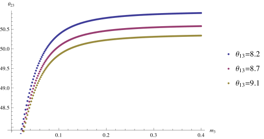
Figure 1: The mixing angle $\theta_{23}$ (in degrees) against the third generation neutrino mass $m_{3}$ (in eV) for various values of the mixing angle $\theta_{13}$ (in degrees).

Actually, there exist solutions for our parameters $(A,B,C,a_{2}^{\prime},a_{3}^{\prime})$ in (109) to realize these experimental values. For example, if we take the parameters to be

$$A =0.00198\,\text{eV},$$ (134)

$$B =30.5,$$

$$C =-5.94,$$

$$a_{2}^{\prime} =-1.09,$$

$$a_{3}^{\prime} =-1.06,$$

we can obtain $m_{3}=0.05\,\text{eV},\theta_{13}=8.7^{\circ},\theta_{23}=49.1^{\circ}$. This solution is also consistent with the $2\sigma$ range of recent fits from neutrinoless double beta decay [28]:

$$m_{\beta\beta} \approx 0.05\text{\,eV},$$ (135)

$$\Sigma =m_{1}+m_{2}+m_{3}\approx 0.15\text{\,eV}.$$ (136)

3.4 Charged lepton masses

Next, we consider the charged lepton mass matrix (85). We want to fix the charged lepton masses as

$$m_{e}=\frac{y^{e}_{l}v_{d}}{\Lambda}\cdot d_{1} =0.5\times 10^{6}\ {\rm eV},$$ (137)

$$m_{\mu}=\frac{y^{e}_{l}v_{d}}{\Lambda}\cdot d_{2} =105\times 10^{6}\ {\rm eV},$$ (138)

$$m_{\tau}=\frac{y^{e}_{l}v_{d}}{\Lambda}\cdot d_{3} =1776\times 10^{6}\ {\rm eV}.$$ (139)

The charged lepton masses are constrained from the D-flatness condition, which for this model is given by

$$\frac{7}{3}e_{1}|d_{1}|^{2}+\frac{7}{3}e_{2}|d_{2}|^{2}+\frac{7}{3}e_{3}|d_{3}|^{2}-\frac{4}{3}e_{1}|b_{1}|^{2}-\frac{4}{3}e_{2}|b_{2}|^{2}-\frac{4}{3}e_{3}|b_{3}|^{2}$$

$$+\frac{2}{3}e_{1}|a_{1}|^{2}+\frac{2}{3}e_{2}|a_{2}|^{2}+\frac{2}{3}e_{3}|a_{3}|^{2}+\frac{1}{3}e_{1}|c_{1}|^{2}=0,$$ (140)

or equivalently

$$+\frac{7}{3}\left(e_{1}|m_{e}|^{2}+e_{2}|m_{\mu}|^{2}+e_{3}|m_{\tau}|^{2}\right)\cdot\left|\frac{\Lambda}{y_{1}^{e}v_{d}}\right|^{2}$$

$$-\frac{4}{3}\left(e_{1}|a_{2}^{\prime}a_{3}^{\prime}A|^{2}+e_{2}\left|\frac{Aa_{3}^{\prime}}{a_{2}^{\prime}}\right|^{2}+e_{3}\left|\frac{Aa_{2}^{\prime}}{a_{3}^{\prime}}\right|^{2}\right)\cdot\left|\frac{\lambda_{1}\Lambda^{2}}{2\lambda_{4}v_{u}^{2}y_{2}^{\nu}}\right|^{2}$$

$$+\frac{2}{3}\left(e_{1}|A|^{2}+e_{2}|a_{2}^{\prime}A|^{2}+e_{3}|a_{3}^{\prime}A|^{2}\right)\cdot\left|\frac{\Lambda^{2}}{v_{u}^{2}y_{2}^{\nu}}\right|^{2}+\frac{1}{3}e_{1}|AC|\cdot\left|\frac{\Lambda^{3}}{y_{3}^{\nu}v_{u}^{2}}\right|=0.$$ (141)

After inserting the solution $(A,B,C,a_{2}^{\prime},a_{3}^{\prime})$ from (134) we can numerically solve (3.4) as a linear equation. Here, we only consider the simplified case where $|\lambda_{1}/(2\lambda_{4})|=1$. Then, we obtain a single solution,

$$\left|\frac{y_{1}^{e}y_{2}^{\nu}}{y_{3}^{\nu}}v_{d}\right| \approx 2.10\text{\,GeV},$$ (142)

$$\left|\frac{(y_{1}^{e})^{2}}{y_{3}^{\nu}}\frac{v_{d}^{2}}{v_{u}^{2}}\Lambda\right| \approx 7.06\times 10^{12}\text{\, GeV}.$$ (143)

Then, by taking “natural” values, $|y_{1}^{e}|=|y_{2}^{\nu}|=|y_{3}^{\nu}|=1$, and by imposing

$$v_{u}^{2}+v_{d}^{2}=(173\text{\,GeV})^{2}$$ (144)

we arrive at

$$\tan\beta =\frac{v_{u}}{v_{d}}\approx 82.4,$$ (145)

$$\Lambda \approx 4.79\times 10^{16}\text{\, GeV}.$$ (146)

Other values of $\tan\beta$ and $\Lambda$ are possible by appropriately adjusting the couplings.

4 Conclusion

In this work, motivated by a gauge origin of discrete symmetries in the framework of the heterotic orbifold models, we have investigated gauge theoretical realizations of non-Abelian discrete flavor symmetries. We have shown that phenomenologically interesting discrete symmetries are realized effectively from a $U(1)^{n}\rtimes S_{m}$ or $U(1)^{n}\rtimes Z_{m}$ gauge theory. These theories can be regarded as UV completions of discrete flavor models. The main difference between a discrete flavor model and a $U(1)$ flavor model as shown in this paper can be seen in the field interactions. Namely, some fields in a discrete flavor model can be distinguished in a $U(1)$ flavor model. For example, the ${\bf 3}_{1(1)}$ representation field of the $\Delta(54)$ symmetry can be described by several $U(1)^{2}$ charges, $(e_{1}/3,e_{2}/3,e_{3}/3)$, $(-2e_{1}/3,-2e_{2}/3,-2e_{3}/3)$ etc. Thus a superpotential in a $U(1)$ flavor model can be different from the one of the corresponding discrete flavor model. In general, $U(1)^{n}\rtimes S_{m}$ and $U(1)^{n}\rtimes Z_{m}$ flavor models are constrained more than flavor models with non-Abelian discrete flavor symmetries, which are subgroups of $U(1)^{n}\rtimes S_{m}$ and $U(1)^{n}\rtimes Z_{m}$, because symmetries are larger. Our results would provide a new insight on flavor models.

We have introduced the specific combination of $U(1)^{2}$ charges, $e_{1}$, $e_{2}$, and $e_{3}$, to realize $S_{4}$, $\Delta(54)$, $A_{4}$ and $\Delta(27)$. They correspond to weights of the triplet (or anti-triplet) representation of $SU(3)$. In fact, $U(1)^{2}\rtimes S_{3}$ is a subgroup of $SU(3)$, where $S_{3}$ is associated with the Weyl group. We also obtained genuine $U(1)^{2}\rtimes S_{3}$ representations which are not obtained from $SU(3)$ triplets by spontaneous symmetry breaking. Also, in a stringy realization of $\Delta(54)$, the $SU(3)$ gauge symmetry appears in toroidal compactification, and the non-zero roots can be projected out by an orbifold projection [20]. This may also suggest that a similar situation can be realized field-theoretically in a higher-dimensional $SU(3)$ gauge theory with a suitable orbifold boundary condition.

Anomalies of non-Abelian discrete symmetries are important [29]. Anomalous discrete symmetries would be violated by non-perturbative effects, but its breaking effects might be small depending on dynamical scales of non-perturbative effects. By our construction, discrete Abelian symmetries originating from $U(1)^{n}$ of $U(1)^{n}\rtimes S_{m}$ and $U(1)^{n}\rtimes Z_{m}$ are always anomaly-free and exact symmetries, but $S_{m}$ and $Z_{m}$ of $U(1)^{n}\rtimes S_{m}$ and $U(1)^{n}\rtimes Z_{m}$ can include anomalous discrete symmetries depending on the model.

We have constructed a concrete flavor model for the lepton sector based on the $U(1)^{2}\rtimes S_{3}$ continuous gauge theory. We have shown that it is possible obtain a realistic flavor structure from this model. Since the model is based on an extended symmetry the number of the parameters is relatively few. In particular, we could show a relation between the angle $\theta_{23}$ and third generation neutrino mass $m_{3}$.

We have shown six types of gauge realizations of non-Abelian discrete symmetries. However, further extensions are possible. For example, extensions to higher $N$, $\Delta(6N^{2})$, is possible if we consider models with $U(1)$ charges $q=e_{i}/N$. It is also possible to include further representations of e.g. $U(1)^{2}\rtimes S_{3}$ which we did not cover here for the sake of simplicity. The general representation theory of these semidirect groups is obtained from the little group method of Wigner, which is familiar from the representation theory of the Poincaré group. Then, e.g. in the case of $U(1)^{2}\rtimes S_{3}$ one obtains an uncharged singlet representation which transforms as ${\bf 1}^{\prime}$ under $S_{3}$ while being uncharged under the $U(1)^{2}$.

A phenomenological implication of our $U(1)$ flavor models is that there should be $Z^{\prime}$ boson(s) which originate from $U(1)$ gauge groups in the effective theory. In this framework $Z^{\prime}$ bosons and flavor structures are related. Since we assigned different $U(1)$ charges to the three-generation leptons, the $Z^{\prime}$ bosons have flavor dependent interactions. Thus, if $Z^{\prime}$ bosons are light as e.g. the TeV scale, they can be a probe of the flavor structure. It will be interesting to investigate $Z^{\prime}$ phenomenology by extending well-known discrete flavor models.

Acknowledgement

S.K. wishes to thank Otto C.W. Kong for helpful discussions. F.B. was supported by the Grant-in-Aid for Scientific Research from the Ministry of Education, Science, Sports, and Culture (MEXT), Japan (No. 23104011). T.K. was supported in part by the Grant-in-Aid for Scientific Research No. 25400252 from the Ministry of Education, Culture, Sports, Science and Technology of Japan. S.K. was supported by the Taiwan’s National Science Council under grant NSC102-2811-M-033-008.

References

• [1] G. Altarelli and F. Feruglio, Rev. Mod. Phys.  82, 2701 (2010) [arXiv:1002.0211 [hep-ph]].
• [2] H. Ishimori, T. Kobayashi, H. Ohki, Y. Shimizu, H. Okada and M. Tanimoto, Prog. Theor. Phys. Suppl.  183, 1 (2010) [arXiv:1003.3552 [hep-th]]; Lect. Notes Phys.  858, 1 (2012); Fortsch. Phys.  61, 441 (2013).
• [3] S. F. King and C. Luhn, Rept. Prog. Phys.  76, 056201 (2013) [arXiv:1301.1340 [hep-ph]].
• [4] L. J. Dixon, J. A. Harvey, C. Vafa and E. Witten, Nucl. Phys.  B 261 (1985) 678; Nucl. Phys.  B 274 (1986) 285.
• [5] L. E. Ibañez, H. P. Nilles and F. Quevedo, Phys. Lett.  B 187 (1987) 25; L. E. Ibañez, J. E. Kim, H. P. Nilles and F. Quevedo, Phys. Lett.  B 191 (1987) 282.
• [6] Y. Katsuki, Y. Kawamura, T. Kobayashi, N. Ohtsubo, Y. Ono and K. Tanioka, Nucl. Phys.  B 341 (1990) 611.
• [7] T. Kobayashi, S. Raby and R. J. Zhang, Phys. Lett.  B 593 (2004) 262 [arXiv:hep-ph/0403065]; Nucl. Phys.  B 704 (2005) 3 [arXiv:hep-ph/0409098].
• [8] W. Buchmüller, K. Hamaguchi, O. Lebedev and M. Ratz, Phys. Rev. Lett.  96 (2006) 121602 [arXiv:hep-ph/0511035]; Nucl. Phys.  B 785 (2007) 149 [arXiv:hep-th/0606187].
• [9] J. E. Kim and B. Kyae, Nucl. Phys.  B 770 (2007) 47 [arXiv:hep-th/0608086].
• [10] O. Lebedev, H. P. Nilles, S. Raby, S. Ramos-Sanchez, M. Ratz, P. K. S. Vaudrevange and A. Wingerter, Phys. Lett. B 645, 88 (2007) [hep-th/0611095]; Phys. Rev. D 77, 046013 (2008) [arXiv:0708.2691 [hep-th]].
• [11] M. Blaszczyk, S. Nibbelink Groot, M. Ratz, F. Ruehle, M. Trapletti and P. K. S. Vaudrevange, Phys. Lett. B 683, 340 (2010) [arXiv:0911.4905 [hep-th]].
• [12] S. Groot Nibbelink and O. Loukas, JHEP 1312, 044 (2013) arXiv:1308.5145 [hep-th].
• [13] H. P. Nilles, S. Ramos-Sanchez, M. Ratz and P. K. S. Vaudrevange, Eur. Phys. J. C 59, 249 (2009) [arXiv:0806.3905 [hep-th]].
• [14] T. Kobayashi, H. P. Nilles, F. Ploger, S. Raby and M. Ratz, Nucl. Phys. B 768, 135 (2007) [hep-ph/0611020].
• [15] H. Abe, K. -S. Choi, T. Kobayashi and H. Ohki, Nucl. Phys. B 820, 317 (2009) [arXiv:0904.2631 [hep-ph]]; Phys. Rev. D 80, 126006 (2009) [arXiv:0907.5274 [hep-th]]; Phys. Rev. D 81, 126003 (2010) [arXiv:1001.1788 [hep-th]].
• [16] M. Berasaluce-Gonzalez, P. G. Camara, F. Marchesano, D. Regalado and A. M. Uranga, JHEP 1209, 059 (2012) [arXiv:1206.2383 [hep-th]]; F. Marchesano, D. Regalado and L. Vazquez-Mercado, JHEP 1309, 028 (2013) [arXiv:1306.1284 [hep-th]].
• [17] Y. Hamada, T. Kobayashi and S. Uemura, JHEP 1405, 116 (2014) [arXiv:1402.2052 [hep-th]].
• [18] T. Higaki, N. Kitazawa, T. Kobayashi and K. j. Takahashi, Phys. Rev. D 72, 086003 (2005) [hep-th/0504019].
• [19] P. Ko, T. Kobayashi, J. -h. Park and S. Raby, Phys. Rev. D 76, 035005 (2007) [Erratum-ibid. D 76, 059901 (2007)] [arXiv:0704.2807 [hep-ph]].
• [20] F. Beye, T. Kobayashi and S. Kuwakino, Phys. Lett. B 736, 433 (2014) [arXiv:1406.4660 [hep-th]].
• [21] H. Abe, K. -S. Choi, T. Kobayashi, H. Ohki and M. Sakai, Int. J. Mod. Phys. A 26, 4067 (2011) [arXiv:1009.5284 [hep-th]].
• [22] C. S. Lam, Phys. Rev. D 78, 073015 (2008) [arXiv:0809.1185 [hep-ph]].
• [23] J. A. Escobar and C. Luhn, J. Math. Phys.  50, 013524 (2009) [arXiv:0809.0639 [hep-th]].
• [24] H. Ishimori, T. Kobayashi, H. Okada, Y. Shimizu and M. Tanimoto, JHEP 0904, 011 (2009) [arXiv:0811.4683 [hep-ph]]; JHEP 0912, 054 (2009) [arXiv:0907.2006 [hep-ph]].
• [25] S. F. King and C. Luhn, JHEP 0910, 093 (2009) [arXiv:0908.1897 [hep-ph]].
• [26] J. A. Escobar, Phys. Rev. D 84, 073009 (2011) [arXiv:1102.1649 [hep-ph]].
• [27] D. V. Forero, M. Tortola and J. W. F. Valle, Phys. Rev. D 90, 093006 (2014) [arXiv:1405.7540 [hep-ph]].
• [28] G. L. Fogli, E. Lisi, A. Marrone, D. Montanino, A. Palazzo and A. M. Rotunno, Phys. Rev. D 86 (2012) 013012 [arXiv:1205.5254 [hep-ph]].
• [29] T. Araki, T. Kobayashi, J. Kubo, S. Ramos-Sanchez, M. Ratz and P. K. S. Vaudrevange, Nucl. Phys. B 805, 124 (2008) [arXiv:0805.0207 [hep-th]].