CHAOS: Accurate and Realtime Detection of Aging-Oriented Failure Using Entropy

Abstract

Even well-designed software systems suffer from chronic performance degradation, also named “software aging”, due to internal (e.g. software bugs) and external (e.g. resource exhaustion) impairments. These chronic problems often fly under the radar of software monitoring systems before causing severe impacts (e.g. system failure). Therefore it’s a challenging issue how to timely detect these problems to prevent system crash. Although a large quantity of approaches have been proposed to solve this issue, the accuracy and effectiveness of these approaches are still far from satisfactory due to the insufficiency of aging indicators adopted by them. In this paper, we present a novel entropy-based aging indicator, Multidimensional Multi-scale Entropy (MMSE). MMSE employs the complexity embedded in runtime performance metrics to indicate software aging and leverages multi-scale and multi-dimension integration to tolerate system fluctuations. Via theoretical proof and experimental evaluation, we demonstrate that MMSE satisfies Stability, Monotonicity and Integration which we conjecture that an ideal aging indicator should have. Based upon MMSE, we develop three failure detection approaches encapsulated in a proof-of-concept named CHAOS. The experimental evaluations in a Video on Demand (VoD) system and in a real-world production system, AntVision, show that CHAOS can detect the failure-prone state in an extraordinarily high accuracy and a near 0 Ahead-Time-To-Failure ($ATTF$). Compared to previous approaches, CHAOS improves the detection accuracy by about 5 times and reduces the $ATTF$ even by 3 orders of magnitude. In addition, CHAOS is light-weight enough to satisfy the realtime requirement.

1 Introduction

Software is becoming the backbone of modern society. Especially with the development of cloud computing, more and more traditional services (e.g. food ordering, retail) are deployed in the cloud and function as distributed software systems. Two common characteristics of those software systems, namely long-running and high complexity increase the risks of faults and resource exhaustion. With the accumulation of faults or resource consumption, software systems may suffer from chronic performance degradation, failure rate/probability increase and even crash called “software aging” [2, 3, 4, 5] or “Chronics” [6].

Software aging has been extensively studied for two decades since it was first quantitatively analyzed in AT&T lab in 1995 [7]. This phenomenon has been widely observed in variant software systems nearly spanning across all software stacks such as cloud computing infrastructure (e.g. Eucalyptus) [8, 9], virtual machine monitor (VMM)[10, 11], operating system[12], Java Virtual Machine (JVM) [5, 13], web server [4, 14] and so on. As the degree of software aging increasing, software performance decreases gradually resulting in QoS (e.g. response time) decrease. What’s worse, software aging may lead to unplanned system hang or crash The unplanned outage in enterprise system especially in cloud platform can cause considerable revenue loss. A recent survey shows that IT downtime on an average leads to 14 hours of downtime per year, leading to $26.5 billion lost [15]. Therefore detecting and counteracting software aging are of essence for building long-running systems.

An efficient and commonly used counteracting software aging strategy is “software rejuvenation” [3, 4, 5, 16], which proactively recovers the system from failure-prone state to a completely or partially new state by cleaning the internal state. The benefit of rejuvenation strategies heavily depends on the time triggering rejuvenation. Frequent rejuvenation actions may decrease the system availability or performance due to the non-ignorable planed downtime or overhead caused by such actions. Instead, an ideal rejuvenation strategy is to recover the system when it just gets near to the failure-prone state.We name the failure-prone state caused by software aging as “Aging-Oriented Failure”(AOF). Different from transient failures caused by fatal errors e.g. segment fault or hardware failures, AOF is a kind of “chronics” [6] which means some durable anomalies have emerged before system crash. Therefore AOF is likely to be detected. Accurately detecting AOF is a critical problem and the goal of this paper. However, to that end, we confront the following three challenges:

• Different from fail-stop problems e.g. crash or hang which have sufficient and observable indicators (e.g. exceptions), non-crash failures caused by software aging where the server does not crash but fails to process the request compliant with the SLA constraints, have no observable and sufficient symptoms to indicate them. These failures often fly under the radar of monitoring systems. Hence, finding out the underlying indicator for software aging becomes the first challenge.

• The internal state (e.g. memory leak) changes and external state (e.g. workload variation) changes make the running system extraordinarily complex. Hence, the running system may not be described neither by a simple linear model nor by a single performance metric. How to cover the complexity and multi-dimension in the aging indicator is the second challenge.

• Fluctuations or noise may be involved in collected performance metrics due to the highly dynamic property of the running system. And cloud computing exacerbates the dynamics due to its elasticity and flexibility (e.g. VM creation and deletion). How to mitigate the influence of noise and keep the detection approach noise-resilient is the third challenge.

To address the aforementioned challenges, we conjecture that an ideal aging indicator should have Monotonicity property to reveal the hidden aging state, Integration property to comprehensively describe aging process and Stability property to tolerate system fluctuation. In this paper, we propose a novel aging indicator named MMSE. According to our observation in practice and qualitative proof, entropy monotonously increases with the degree of software aging when the failure probability is lower than 0.5. And MMSE is a complexity oriented and model-free indicator without deterministic linear or non-linear model assumptions. In addition, the multi-scale feature mitigates the influence of system fluctuations and the multi-dimension feature makes MMSE more comprehensive to describe software aging. Hence, MMSE satisfies the three properties namely Stability, Monotonicity and Integration, which we conjecture that an ideal aging indicator should have. Based upon MMSE, we develop three AOF detection approaches encapsulated in a proof-of-concept, CHAOS. To further decrease the overhead caused by CHAOS, we reduce the runtime performance metrics from 76 to 5 without significant information loss by a principal component analysis (PCA) based variable selection method. The experimental evaluations in a VoD system and in a real production system, AntVision , show that CHAOS has a strong power to detect failure-prone state with a high accuracy and a small $ATTF$. Compared to precious approaches CHAOS increases the detection accuracy by about 5 times and reduces the $ATTF$ significantly even by 3 orders of magnitude. According to our best knowledge, this is the first work to leverage entropy to indicator software aging. The contribution of this paper is three-fold:

• We demonstrate that entropy increases with software aging and verify this conclusion via experimental practice and quantitative proof.

• We propose a novel aging indicator named MMSE. MMSE employs the complexity embedded in multiple runtime performance metrics to measure software aging and leverages multi-scale and multi-dimension integration to tolerate system fluctuations ,which makes MMSE satisfy the properties: Stability, Monotonicity and Integration.

• We design and implement a proof-of-concept named CHAOS, and evaluate the accuracy of three failure detection approaches based upon MMSE encapsulated in CHAOS in a VoD system and a real production system, AntVision. The experimental results show that CHAOS improves the detection accuracy by about 5 times and reduces the $ATTF$ by 3 orders of magnitude compared to previous approaches.

The rest of this paper is organized as follows. We demonstrate the motivations of this paper in Section II. Section III shows our solution to detect the failure-prone state and the overview of CHAOS. And in Section IV, we describe the detailed design of CHAOS including: metric selection, MSE and MMSE calculation procedure, and failure-prone state detection approaches. Section V shows the evaluation results and comparisons to previous approaches. In Section VI we state the related work briefly. Section VII concludes this paper.

2 Motivation

The accuracy of Aging-Oriented Failure (AOF) detection approaches is largely determined by the aging indicators. A well-designed aging indicator can precisely indicate the AOF. If the subsequent rejuvenations are always conducted at the real failure-prone state, the rejuvenation cost will tend to be optimal. But unfortunately, prior detection approaches based upon explicit aging indicators [2, 4, 5, 14, 17, 18] don’t function well especially in the face of dynamic workloads. They either miss some failures leading to a low recall or mistake some normal states as the failure states leading to a low precision. The insufficiency of previous indicators motivates us to seek novel indicators. We describe our motivations from the following aspects.

2.1 Insufficiency of Explicit Aging Indicators

To distinguish the normal state and failure-prone state, a threshold should be preset on the aging indicator. Once the aging indicator exceeds the threshold, a failure occurs. Traditionally, a threshold is set on explicit aging indicators. For instance, if the CPU utilization exceeds $90\%$, a failure occurs. However, it’s not always the case. The external observations do not always reveal accurately the internal states. Here the internal states can be referred to as some normal events (e.g. a file reading, a packet sending) or abnormal events (e.g. a file open exception, a round-off error) generated in the system. In this paper we are more concerned about the abnormal events. Commonly, the internal state space is much smaller than the directly observed external state space. For example, the observed CPU utilization can be any real number in the range $0\%\sim 100\%$ while the abnormal events are very limited. Therefore an abnormal event may correlate with multiple observations. Still take the CPU utilization for example. When a failure-prone event happens, the CPU utilization may be 99%, 80% or even 10%. Therefore the explicit aging indicator can not signify AOF sufficiently and accurately. And if the system fluctuation is taken into account, the situation may get even worse. And this is also a reason why it’s so difficult to set an optimal threshold on the explicit aging indicators in order to obtain an accurate failure detection result.

2.2 Entropy Increase in VoD System

As the explicit aging indicators fall short in detecting Aging-Oriented Failure, we turn to implicit aging indicators for help. Some insights can be attained from [19] and [14]. Both of them treated software aging as a complex process. Motivated by them, we believe entropy as a measurement of complexity has a potential to be an implicit aging indicator.

In a real campus VoD (Video on Demand) system which is charge of sharing movies amongst students, we observe that entropy increases with the degree of software aging. The VoD system runs for 52 days until a failure occurs. By manually investigating the reason of failure, we assure it is an Aging-Oriented Failure. During the system running, the CPU utilization is recorded to be processed later shown in Figure 1. We adopt MSE to calculate the entropy value of the CPU utilization of each day. The result is demonstrated in Figure 2. Figure 2 only shows the entropy value of the first four days ($Day1,Day2,Day3,Day4$) and the last four days ($Day49,Day50,Day51,Day52$). It’s apparent to see the entropy values of the last four days are much larger than the ones of the first four days nearly at all scales. Especially, the entropy value of Day52 when the system failed is different significantly from others. However the raw CPU utilization at failure state seems normal which means we may not detect the failure state if using this metric as an aging indicator. Therefore, MSE seems a potential aging indicator in this practice.

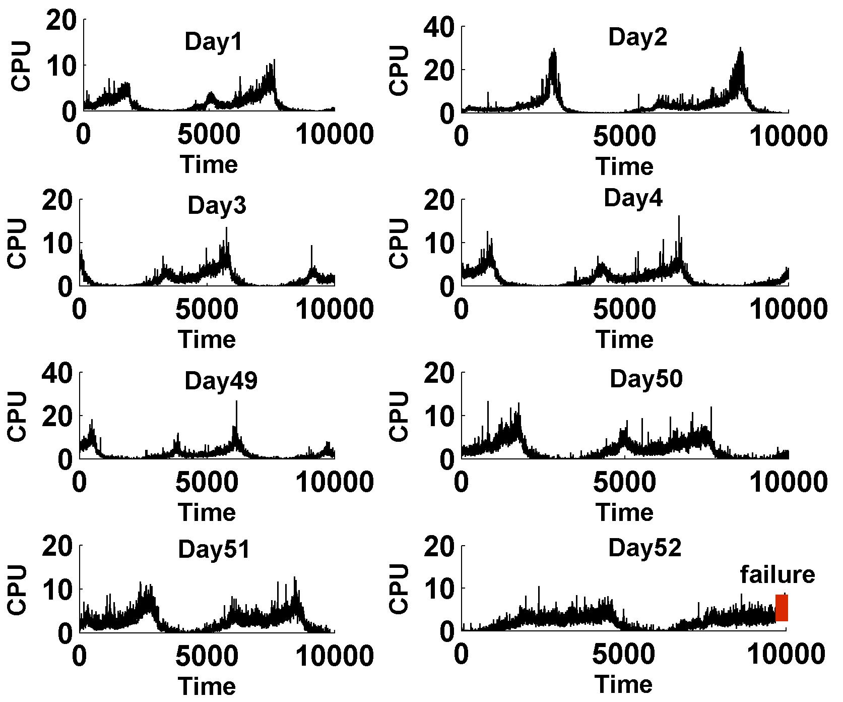
Figure 1: The CPU utilization of a real VoD system. In this figure, we only show the CPU utilization of the first four days and the last four days.

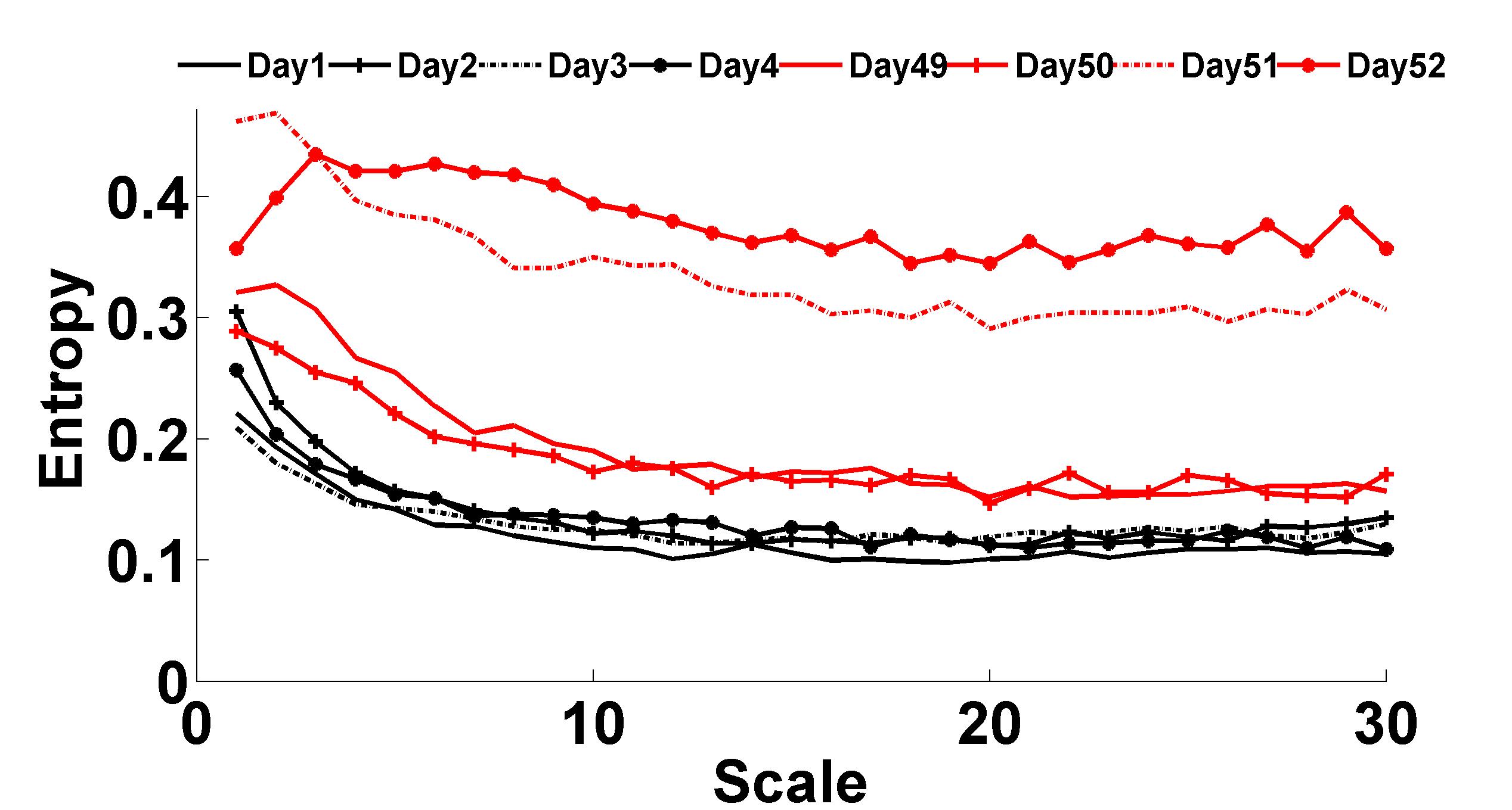
Figure 2: The entropy value of a real VoD system at 30 scales

2.3 Conjecture

According to the above observation, we provide a high level abstraction of the properties that an ideal aging indicator should satisfy. Monotonicity: Since software aging is a gradual deterioration process, the aging indicator should also change consistently with the degree of software aging, namely increase or decrease monotonically. As the most essential property, monotonicity provides a foundation to detect Aging-Oriented Failure accurately. Stability: The indicator is capable of tolerating the noise or disturbance involved in the runtime performance metrics. Integration: As software aging is a complex process affected by multiple factors, the indicator should cover these influence from multiple data sources, which means it is the integration of multiple runtime metrics.

It’s worth noting that the property set my not be complete, any new property which can strength the detection power of aging indicators can be complemented. In a real-world system, it is extraordinarily hard to find such an ideal aging indicator. But it is possible to find a workaround which is close to the ideal indicator.

3 Solution

To provide accurate and effective approaches to detect AOF, the first step is to propose an appropriate aging indicator satisfying the three properties mentioned in section II.C. As described in the motivation, we find out MSE seems a potential indicator. But to satisfy all the three properties we proposed, some proofs and modifications are necessary. First of all, we need to quantitatively prove that entropy caters to $Monotonicity$ in software aging procedure which is illustrated in Appendix A. The proof tells us the system entropy increases with the degree of software aging when the probability of failure state ($p_{f}$) is smaller than the probability of working state ($p_{w}$). In most situations, the system can’t provide acceptable services or goes to failure very soon once $p_{w}<p_{f}$. Therefore we only take into account the scenario with a constraint $p_{w}>p_{f}$. Under this constraint, the $Monotonicity$ of entropy in software aging is proved. However, the strict monotonicity could be biased a little due to the ever-changing runtime environment. Because of the inherent “multi-scale” nature of MSE, the $Stability$ property is strengthened. Via multi-scale transformation, some noises are filtered or smoothed. In addition, the combination of entropy at multiple scales further mitigates the influence of noises. The last but not the least property is $Integration$. Unfortunately, MSE is originally designed for analyzing single dimensional data rather than multiple dimensional data. Thus, to satisfy integration property, we extend the original MSE to MMSE via several modifications. Finally, we achieve a novel software aging indicator, MMSE, which satisfies all the three properties. Based upon MMSE, we have implemented threshold based and time series based methods to detect AOF. To evaluate the effectiveness and accuracy of our approaches, we design and implement a proof-of-concept named CHAOS. The details of CHAOS will be depicted in next section.

4 System Design

The architecture of CHAOS is shown in Figure 3. CHAOS mainly contains four modules: data collection, metric selection, MMSE calculation and crash detection. The data collection module collects runtime performance metrics from multiple data sources including application (e.g. response time), process (e.g. process working set) and operating system (e.g. total memory utilization). Amongst the raw performance metrics, collinearity is thought to be common which means some metrics are redundant. What’s worse, a significant overhead is caused if all of performance data is analyzed by the MMSE calculation module. Thus, a metric selection module is necessary to select a subset of the original metrics without major loss of quality. The selected metric subset is fed into MMSE calculation module to calculate the sample entropy at multiple scales in real time. Then the entropy values are adopted to detect AOF by the crash detection module. The final result of CHAOS is a boolean value indicating whether failure-prone state occurs. We will demonstrate the details in the following parts.

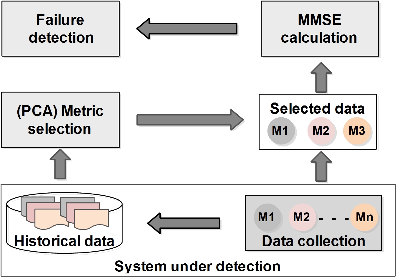
Figure 3: The architecture of CHAOS

4.1 Metric Selection

To get rid of the collinearity amongst the high-dimensional performance metrics and reduce computational overhead, we select a subset of metrics which can be used as a surrogate for a full set of metrics, without significant loss of information. Assume there are $M$ metrics, our goal is to select the best subset of any size $k$ from 1 to $M$. To this end, PCA (Principal Component Analysis) variable selection method is introduced.

As a classical multivariate analysis approach, PCA is always used to transform orthogonally a set of variables which may be correlated to a set of variables which are linearly uncorrelated (i.e. PC). let X denote a column centered $n$x$M$ matrix, where $M$ denotes the number of metrics, $n$ denotes the number of observations. Via PCA, the matrix X could be reconstructed approximately by $p$ PCs, where $p\ll M$. These PCs are also called latent factors which are given new physical meanings. Mathematically, X is transformed into a new $n$x$k$ matrix of principal component scores T by a loading or weight $k$x$M$ matrix W if keeping only the $k$ principal component, namely $\textbf{T}=\textbf{X}{{\textbf{W}}^{T}}$ where each column of T is called a PC. The loading factor W can be obtained by calculating the eigenvector of ${{\textbf{X}}^{T}\textbf{X}}$ or via singular value decomposition (SVD)[20]. In stead, we leverage PCA to select variables rather than reduce dimensions.

In order to achieve that goal, we first introduce a well-defined numerical criteria in order to rank the subset of variables. Here choose GCD [21, 22] as a criteria. GCD is a measurement of the closeness of two subspaces spanned by different variable sets. In this paper, GCD is a measure of similarity between the principal subspace spanned by the $k$ specified PCs and the subspace spanned by a given $p$-variable subset of the original $M$-variable data set. By default, the specified PCs are usually the first $k$ PCs and the number of variables and PCs is the same ($k=p$). The detailed description of GCD could be found in [21].

Then we need a search algorithm to seek the best $p$-variable subset of the full data set. In this paper, we adopt a heuristic simulated annealing algorithm to search for the best p-variable subset. The algorithm is described in detail in [23]. In brief, an initial p-variable subset is fed into the simulated annealing algorithm, then the GCD criterion value is calculated. Further, a subset in the neighborhood of the current subset is randomly selected. The alternative subset is chosen if its GCD criteria value is larger than the one of the current subset or with a probability $e^{\frac{ac-cc}{t}}$ if the GCD criteria value of the alternative subset (ac) is smaller than the one of current subset (cc) where $t$ denotes the temperature and decreases throughout the iterations of the algorithm. The algorithm stops when the number of iterations exceeds the preset threshold. The merit of the simulated annealing algorithm is that the best p-variable subset can be obtained with a reasonable computation overhead even the number of variables is very large.

With the well-defined GCD criteria and the simulated annealing search algorithm, we can reduce the high-dimensional runtime performance metrics (e.g. 76) to very low-dimensional data set (e.g. 5) with very little information loss. And the computation overhead is decreased significantly.

4.2 Proposed Multidimensional Multi-scale Entropy

A well-known measurement of system complexity is the classical Shannon entropy [24]. However, Shannon entropy is only concerned with the instant entropy at a specific time point. It can’t capture the temporal structures of one time series completely leading to statistical characteristic loss and even false judgment. MSE proposed by Costa et al [25] is used to quantify the amount of structures (i.e. complexity) embedded in the time series at multiple time scales. A system without structures would exhibit a significant entropy decrease with an increasing time scale. The algorithm of MSE includes two phases:sample entropy [26] calculation and coarse-graining. Given a positive number $m$, a random variable $X$ and a time series $\textbf{X}=\{X(1),X(2),\cdots,X(N)\}$ with length $N$, X is partitioned into consecutive segments. Each segment is represented by a $m$-length vector: $u_{m}(t)=\{x(t),X(t+1),\cdots,X(t+m-1)\},1\leq t\leq N-m+1$ where $m$ could be recognized as the embedded dimension and recommended as $m=2$ [27]. let $n_{i}^{m}(r)$ denote the number of segments that satisfy $d(u_{m}(i),u_{m}(j))\leq r,i\neq j$ where $i\neq j$ guarantees that self-matches are excluded, $r$ is a preset threshold indicating the tolerance level for two segments to be considered similar and recommended as $r=1.5*\sigma$ [27] where $\sigma$ is the standard deviation of the original time series. $d(\cdot)=max\{|X(i+k)-X(j+k)|:1\leq k\leq m-1\}$ represents the maximum of the absolute values of differences between $u_{m}(i),u_{m}(j)$ measured by Euclidean distance which is adopted in this paper Let $lnC_{i}^{m}(r)=ln\frac{u_{m}(i)}{N-m}$ represent the natural logarithm of the probability that any segment $u_{m}(j)$ is close to segment $u_{m}(i)$, the average of $lnC^{m}(r)$ is expressed as:

$$\Phi^{m}(r)=\frac{\sum_{i}^{N-m+1}lnC_{i}^{m}(r)}{N-m+1}$$ (1)

The sample entropy is formalized as:

$$S_{E}(m,r,N)=-ln\frac{\Phi^{m+1}(r)}{\Phi^{m}(r)}$$ (2)

To ensure $\Phi^{m+1}(r)$ is defined in any particular $N$-length time series, sample entropy redefines $\Phi^{m}(r)$ as:

$$\Phi^{m}(r)=\frac{\sum_{i}^{N-m}lnC_{i}^{m}(r)}{N-m}$$ (3)

Suppose $\tau$ is the scale factor, the consecutive coarse-grained time series $Y^{\tau}$ is constructed in the following two steps:

• Divide the original time series X into consecutive and non-overlapping windows of length $\tau$;

• Average the data points inside each window;

Finally we get $Y^{\tau}=\{y_{j}^{\tau}|:1\leq j\leq\lfloor\frac{N}{\tau}\rfloor\}$ and each element of $Y^{\tau}$ is defined as:

$$y_{j}^{\tau}=\frac{\sum_{i=(j-1)\tau+1}^{j\tau}X(i)}{\tau},1\leq j\leq\lfloor\frac{N}{\tau}\rfloor$$ (4)

When $\tau=1$, $Y^{\tau}$ degenerates to the original time series X. Then MSE of the original time series X is obtained by computing the sample entropy of $Y^{\tau}$ at all scales. However, the conventional MSE is designed for single dimensional analysis. Thus, it doesn’t satisfy the property Integration of an aging indicator. To this end, we extend MSE to MMSE via several modifications.

Modification 1. The collected multi-dimensional performance metrics usually have different scales and numerical ranges. For example the CPU utilization metric stays in the range of 0 $\sim$ 100 percentage while the total memory utilization may vary in the range 1048576KB $\sim$ 4194304 KB. Thus, the distance between two segments may be biased by the performance metrics with large numerical ranges, which further results in MSE bias. To avoid that bias, we normalize all the performance metrics to a unified numerical range,namely $0\sim 1$. Suppose $X$ is a $Nxp$ data matrix where $p$ is the number of performance metrics, $N$ is the length of the data window and each column of $X$ denotes the time series of one particular performance metric, then $X$ is normalized in the following way:

$$X_{ji}^{{}^{\prime}}=\frac{X_{ji}-min(X_{i})}{max(X_{i})-min(X_{i})},1\leq i\leq p,1\leq j\leq N$$ (5)

Modification 2. In MSE algorithm, we quantify the similarity between two segments via maximum norm [28] of two scalar numbers. A novel quantification approach is necessary when MSE is extended to MMSE. Each element in the maximal norm pair: $max\{|X(i+k)-X(j+k)|:1\leq k\leq m-1\}$ such as $X(i+k)$ is replaced by a vector $\textbf{X}(i+k)$ where each element represents the observation of one specific performance metric at time $i+k$. Thus the scalar norm is transformed to the vector norm. The embedded dimension $m$ should also be vectorized when the analysis shifts from single dimension to multiple dimensions. The vectorization brings a nontrivial problem in the calculation procedure of sample entropy that is how to obtain $\phi^{m+1}(r)$. Assume that the embedding vector $\textbf{m}=(m_{1},m_{2},\cdots,m_{p})$ denotes the embedded dimensions for $p$ performance metrics respectively. A new embedding vector $\textbf{m}^{+}$ which has one additional dimension compared to m can be obtained in two ways. The first approach comes from the study in [28]. According to the embedding theory mentioned in [29], $\textbf{m}^{+}$ can be achieved by adding one additional dimension to only one specific embedded dimension in m, which leads to $p$ different alternatives. $\textbf{m}^{+}$ can be any one of the set $\{(m_{1},m_{2},\cdots,m_{k}+1,\cdots,m_{p}),1\leq k\leq p\}$. $\phi^{\textbf{m}^{+}}(r)$ is calculated in a naive way or a rigorous way both of which are depicted in detail in [28]. The other approach is very simple and intuitional that is adding one additional dimension to every embedded dimension in m. There is only one alternative for $\textbf{m}^{+}$ namely $\{(m_{1}+1,m_{2}+1,\cdots,m_{k}+1,\cdots,m_{p}+1),1\leq k\leq p\}$ . This simple approach implies that each embedded dimension is identical, which may be a strong constraint. However, compared to the former approach, the latter one has negligible computation overhead and works well in this paper. The former approach will be discussed in our future work.

Modification 3. In MSE algorithm, the threshold $r$ is set as $r=0.15*\sigma$.In MMSE algorithm, we need a single number to represent the variance of the multi-dimensional performance data in order to apply it directly in the similarity calculation procedure. Here we employ the total variance denoted by $tr(\textbf{S})$ which is defined as the trace of the covariance S of the normalized multi-dimensional performance data to replace $\sigma$.

Modification 4. We argue that an ideal aging indicator should be expressed as a single number in order to be readily used in failure detection. The output of the conventional MSE is a vector of entropy values at multiple scales. We need to use a holistic metric to integrate all the entropy values at multiple scales. Thus a composed entropy (CE) is proposed. Let $T$ denote the number of scales and the vector $\textbf{E}=(e_{1},e_{2},\cdots,e_{T})$ denote the entropy value at each scale respectively. Then $CE$ is defined as the Euclidean norm of the entropy vector E :

$$CE=\sqrt[2]{\sum_{i=1}^{T}e_{i}^{2}}$$ (6)

$CE$ cloud be regarded as the Euclidean distance between E and a “zero” entropy vector which consists of $0$ entropy values. A “zero” entropy vector represents an ideal system state meaning that the system runs in a health state without any fluctuations. Thus the more E deviates from a “zero” entropy vector, the worse the system performance is. It’s worth noting that $CE$ is not the unique metric which can integrate the entropy values at all scales. Other metrics also have the potential to be the aging indicators. For example, the average of E is another alternative although we observe that it has a consistent result with $CE$.

Through the aforementioned modifications on MSE, the novel aging indicator MMSE has satisfied all the three properties: Monotonicity, Stability and Integration proposed in Section II.C. For the sake of clarity, we demonstrate the pseudo code of MMSE algorithm in Algorithm 1.

Algorithm 1 MMSE algorithm

0:  $m$:the embedded dimension; $T$:the number of scales; $N$:the length of data window; X: a $N$x$p$ data matrix where each $p$ denotes the number of performance metrics and each column $X_{i},1\leq i\leq p$ denotes the time series of one specific performance metric with length $N$.

0:  The aging degree metric $CE$

1:  $//$ Normalize the original time series into the range [0,1]

2:  for $j=1;j=N;j++$ do

3:     for $i=1;i=p;i++$ do

4:        $X_{ji}^{{}^{\prime}}=\frac{X_{ji}-min(X_{i})}{max(X_{i})-min(X_{i})}$

5:     end for

6:  end for

7:  $//$ Preset the similarity threshold $r$

8:  $S=Cov(X^{{}^{\prime}})$ $//$ $Cov$ denotes the matrix covariance

9:  $r=tr(S)$ $//$ $tr$ denotes the trace of a particular matrix

10:  for $\tau=1;\tau=T;\tau++$ do

11:     $//$ Coarse-graining procedure

12:     for $i=1;i=p;i++$ do

13:        for $j=1;j=\lfloor\frac{N}{\tau}\rfloor;j++$ do

14:           $Y_{ji}=\frac{\sum_{k=(j-1)\tau+1}^{j\tau}X_{ki}^{{}^{\prime}}}{\tau}$

15:        end for

16:     end for

17:     $E(\tau)=ExtendedSampleEntropy(m,r,Y)$

18:     $//$ The similarity calculation between two

19:     $//$ segments has been extended from scalar

20:     $//$ to vector in $ExtendedSampleEntropy(\cdot)$

21:  end for

22:  $//$ Calculate the composed entropy $CE$

23:  $CE=\sqrt[2]{\sum_{i=1}^{T}E(i)^{2}}$

4.3 AOF Detection based upon MMSE

Based upon the proposed aging indicator MMSE, it’s easy to design algorithms to detect AOF in real time. According to the survey [30], there are three kinds of approaches including time series analysis,threshold-based and machine learning to detect or predict the occurrence of AOF.In this paper, we only discuss the time series and threshold-based approaches and leave the machine learning approach in our future work. But before that we need to determine a sliding data window in order to calculate MMSE in real time. As mentioned in previous work [31], $\lfloor\frac{N}{\tau}\rfloor$ should stay in the range $10^{m}$ to $30^{m}$. Thus the sliding window heavily depends on the scale factor $\tau$. In previous studies [32, 25, 28], they usually set the scale factor $\tau$ in the range $1\sim 20$ leading to a huge data window, say 10000, especially when $\tau=20$. A large sliding window not only increases the computational overhead but also makes detection approaches insensitive to failure. Thus we constrain the sliding window in an appropriate range, say no more than 1000, by limiting the range of $\tau$. In this paper we set $\tau$ in the range $1\sim 10$. So a moderate data window $N=1000$ can cater the basic requirement.
Threshold based approach. As a simple and straightforward approach, the threshold based approach is widely used in aging failure detection [33, 34]. If the aging indicator exceeds the preset threshold, a failure occurs. However an essential challenge is how to identify an appropriate threshold. Identifying the threshold from the empirical observation is a feasible approach. This approach learns a normal pattern when the system runs in the normal state. If the normal pattern is violated, a failure occurs. We call this approach $FailureThreshold$ ($FT$). Assume that $\textbf{CE}=\{CE(1),CE(2),CE(3),\cdots,CE(n)\}$ represents a series of normal data where each element $CE(t)$ denotes a $CE$ value at time $t$. The failure threshold $ft$ is defined as: $ft=\beta*max(\textbf{CE})$ where $\beta$ is a tunable fluctuation factor which is used to cover the unobserved value escaped from the training data. As mentioned above, MMSE increases with the degree of software aging. Thus a failure occurs only when the new observed $CE$ exceeds $ft$, something like upper boundary test. For the aging indicators which have a downtrend such as AverageBandwidth, the $max$ function in (9) will be replaced by $min$, something like lower boundary test. A failure occurs if the new observed $CE$ is lower than $ft$.

$FT$ can be further extended to be an incremental version named $FT$-$X$ in order to adapt to the ever changing running environment. $FT$-$X$ learns $ft$ incrementally from historical data. Once a new $CE(t+1)$ is obtained and the system is assured to stay in the normal state, then we compare $CE(t+1)$ with previously trained $max(\textbf{CE}(t))$. If $CE(t+1)<max(\textbf{CE}(t))$ then $ft=\beta*max(\textbf{CE})$ else $ft=\beta*CE(t+1)$. Besides the realtime advantage, $FT$-$X$ needs very little memory space to store the new $CE$ and previously trained maximum of CE.
Time series approach. Although the threshold based approach is simple and straightforward, identifying the threshold is still a thorny problem. Thus, to bypass the threshold setting dilemma, we need a time series approach which requires no threshold or adjusts a threshold dynamically. To compare with existing approaches, we leverage the extended version of Shewhart control charts algorithm proposed in [19] to detect AOF. But one difference exists. In [19], they adopt the deviation $d_{n}$ between the local average $a_{n}$ and the global mean $\mu_{n}$ to detect aging failures. $d_{n}$ is defined as:

$$d_{n}=\frac{\sqrt[2]{N^{{}^{\prime}}}}{\sigma_{n}}(\mu_{n}-a_{n})$$ (7)

where $N^{{}^{\prime}}$ is used to represent the sliding window on entropy data calculated by MMSE algorithm in order to distinguish it from the sliding window $N$ in MMSE algorithm, the meaning of other relevant parameters can be found in [19]. They pointed out that $H\ddot{o}lder$ exponent decreased with the degree of software aging. Therefore they only took into account the scenario of $\mu_{n}>a_{n}$. In this paper, we prove that MMSE increases with the degree of software aging. Thus we only take into account the scenario of $\mu_{n}<a_{n}$. $d_{n}$ is redefined as:

$$d_{n}=\frac{\sqrt[2]{N^{{}^{\prime}}}}{\sigma_{n}}(a_{n}-\mu_{n})$$ (8)

If $d_{n}>\epsilon$ holds for $p$ consecutive points where $\epsilon$ and $p$ are tunable parameters, a change occurs. We insist that a change is assured when $p=4$ at least in this paper. So $N^{{}^{\prime}}$ and $\epsilon$ are the primary factors affecting the detection results. In [19], the second change in $H\ddot{o}lder$ exponent implies a system failure. By observing the MMSE variation curves obtained from Helix Server test platform and real-world AntVision system shown in Section VI, we find out that these curves can be roughly divided into three phases: slowly rising phase, fast rising phase and failure-prone phase. And when the system steps into the failure-prone phase, a failure will come soon. Therefore we also assume that the second change in MMSE data implies a system failure.

5 Experimental Evaluation

We have designed and implemented a proof-of-concept named CHAOS and deployed it a controlled environment. To monitor the common process and operating system related performance metrics such as CPU utilization and context switch, we employ some off-the-shelf tools such as Windows Performance Monitor shipped with Window OS or Hyperic [35]; to monitor other application related metrics such as response time and throughput, we develop several probes from scratch The sampling interval in all the monitoring tools is 1 minute. Next, we will demonstrate the details of our experimental methodology and evaluation results in a VoD system, Helix Server and in a real production system, AntVision.

5.1 Evaluation Methodology

To make comprehensive evaluations and comparisons from multiple angels, we deploy CHAOS in a VoD test environment. And to evaluate the effectiveness of CHAOS in real world systems, we use CHAOS to detect failures in AntVision system.

VoD system. We choose VoD system as our test platform because more and more services involve video and audio data transmission. What’s more, the “aging” phenomenon has been observed in such kinds of applications in our previous work [36, 37]. We leverage Helix Server [38] as a test platform to evaluate our system due to its open source and wide usage. Helix Server as a mainstream VoD software system is adopted to transmit video and audio data via RTSP/ RTP protocol. At present, there are very few VoD benchmarks. Hence, we develop a client emulator named $HelixClientEmulator$ employing RTSP and RTP protocols from scratch. It can generate multiple concurrent clients to access media files on a Helix Server. Our test platform consists of one server hosting Helix Server, three clients hosting $HelixClientEmulator$ and one Gigabit switch connecting the clients and the server together. 100 rmvb media files with different bit rates are deployed on the Helix Server machine. Each client machine is configured with one Intel dual core 2.66Ghz CPU and 2 GB memory and one Gigabit NIC and runs 64-bit Windows 7 operating system. The server machine is configured with two 4-core Xeon 2.1 GHZ CPU processors, 16GB memory, a 1TB hard disk and a Gigabit NIC and runs 64-bit Windows server 2003 operating system.

During system running, thousands of performance counters can be monitored. In order to trade off between monitoring effort and information completeness, this paper only monitors some of the parameters at four different levels: Helix Client, OS, Helix Server, and server process via respective probes shown in Figure 6. From Helix Client level, we record the performance metrics such as Jitter, Average Response Time and etc via the probes embedded in $HelixClientEmulator$; from OS level, we monitor Network Transmission Rate, Total CPU Utilization and etc via Windows Performance Monitor; from Helix Server level, we monitor the application relevant metrics such as Average Bandwidth Output Per Player(bps), Players Connected and etc from the log produced by Helix Server; from process level, we monitor some of metrics related to the Helix Server process like Process Working Set via Windows Performance Monitor.Due to the limited space, we will not show the 76 performance metrics.

AntVision System. Besides the evaluations in a controlled environment, we further apply CHAOS to detect failures in AntVision system. AntVision is a complex system which is used to monitor and analyze public opinions and information from social networks like Sina Weibo. The whole system consists of hundreds of machines in charge of crawling information, filtering data, storing data and etc. More information about this system can be found in $www.antvision.net$. With the help of system administrators, we have obtained a $7$-$day$ runtime log from AntVision. The log data not only contain performance data but also failure reports. Although the performance data only involve two metrics i.e. CPU and memory utilization, it’s enough to evaluate the failure detection power of CHAOS. According to the failure reports, we observe that one machine crashed in the 6th day without knowing the reason. After manual investigation, we conclude that the outage is likely caused by software aging.

In the controlled environment, we conducted 50 experiments. In each experiment, we guarantee the system runs to “failure”. Here “failure” not only refers to system crashes but also QoS violations.In this paper, we leverage Average Bandwidth Output Per Player(bps) (AverageBandwidth) as the QoS metric. Once AverageBandwidth is lower than a preset threshold e.g. 30bps for a long period, a “failure” occurs because a large number of video and audio frames are lost at that moment. To get the ground truth, we manually label the “failure” point for each experiment. However due to the interference of noise and ambiguity of manual labeling, the failure detection approaches may report failures around the labeled “failure” point rather than at the precise “failure” point. Thus we determine that the failure is correctly detected if the failure report falls in the “decision window”. The decision window with a specific length (e.g. 100 in this paper)is defined as a data window whose right boundary is the labeled “failure” point.

Four metrics are employed to quantitatively evaluate the effectiveness of CHAOS. They are $Recall$, $Precision$, $F1$-$measure$ and $ATTF$. The former two metrics are defined as:

$$Recall=\frac{N_{tp}}{N_{tp}+N_{fn}},Precision=\frac{N_{tp}}{N_{tp}+N_{fp}}$$

where $N_{tp}$, $N_{fn}$, and $N_{fp}$ denote the number of true positives, false negatives, and false positives respectively. It’s worth noting that $N_{tp}$, $N_{fn}$, $N_{fp}$ are the aggregated numbers over 50 experiments respectively. To represent the accuracy in a single value, $F1$-$measure$ is leveraged and defined as:

$$F1-measure=\frac{2*Recall*Precision}{Recall+Precision}$$

$ATTF$ is defined as the time span between the first failure report and the real failure namely the left boundary of the decision window in this paper. In a real-world system, once a failure is detected the system may be rebooted or offloaded for maintenance. Thus we choose the first failure report as a reference point. If the first failure report falls in the decision window, $ATTF=0$. A large $ATTF$ may cause excessive system maintenance leading to availability decrease and operation cost increase. Therefore a lower $ATTF$ is preferred.

5.2 Performance Metric Selection

By investigating all the performance metrics, we find that many metrics have very similar characteristics like trend meaning these metrics are highly correlated. Therefore we select a small subset of metrics which can be used as a surrogate of the full data set without significant information loss via PCA variable selection presented in Section V.A. We calculate the best GCD scores of different variable sets with specific cardinalities (e.g. $k=3$) by the simulated annealing algorithm. Figure 4 shows the variation of the best GCD sore along with the number of variables. From this figure, we observe that the GCD score doesn’t increase significantly any more when the number of variables reaches 5. Therefore these 5 variables are already capable of representing the full data set. The 5 variables are Total CPU Utilization, AverageBadwidth, Process IO Operations Per Second , Process Virtual Bytes Peak, Jitter respectively. In the following experiments, we will use them to evaluate CHAOS.

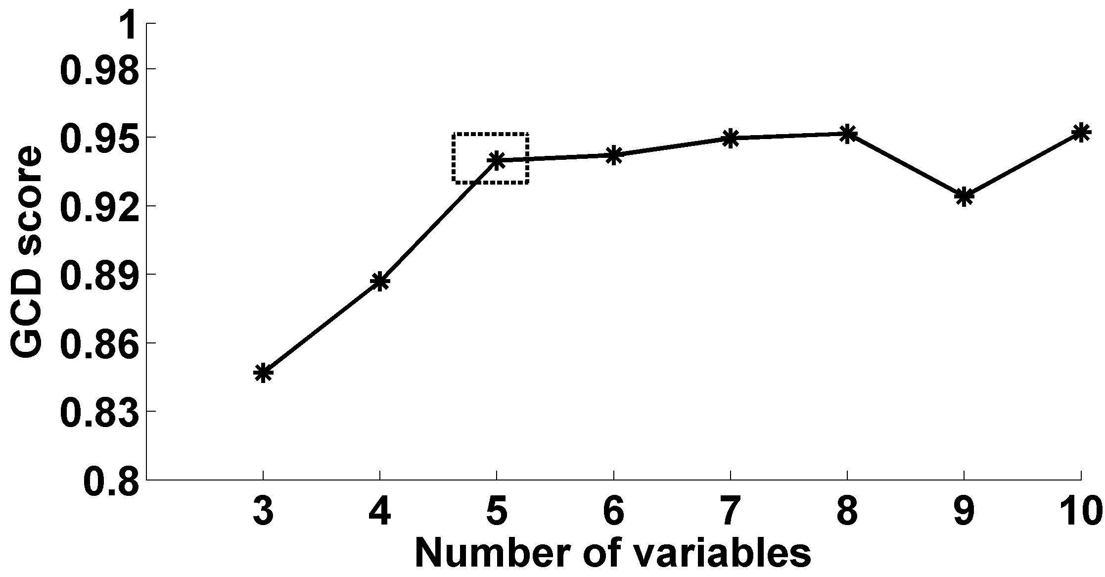
Figure 4: The variation of GCD sore along with the number of variables

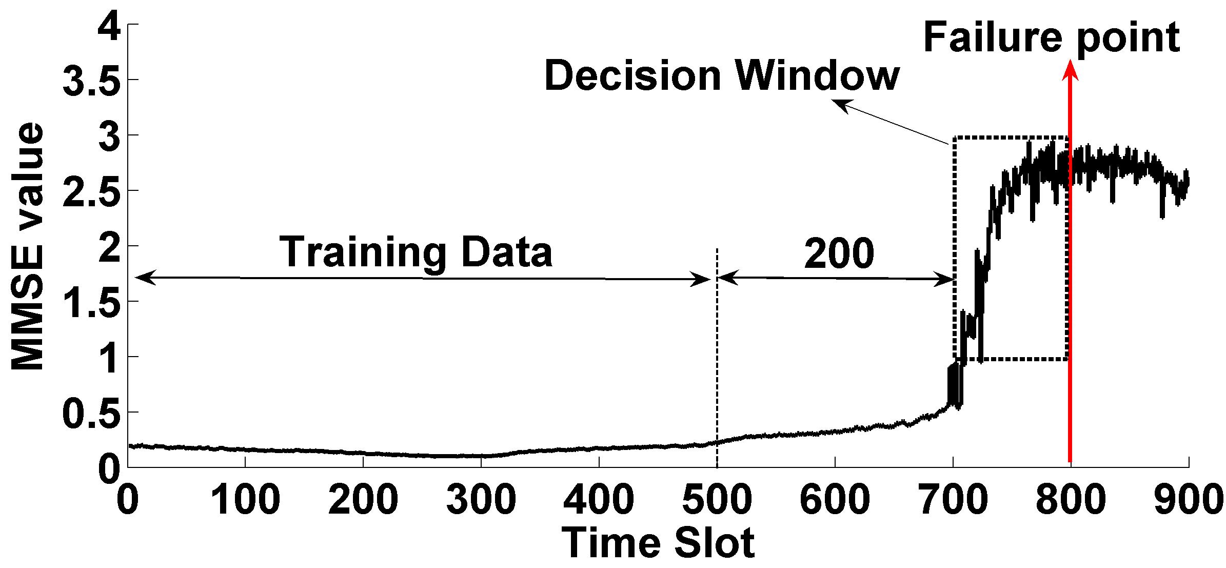
Figure 5: Training data selection in $FT$ approach.

5.3 AOF Detection

In this section, we will demonstrate the the failure detection results of CHAOS. In MMSE algorithm, we set the embedded dimension $m=2$, the sliding window $N=1000$,the number of scales $T=10$. For the failure detection approach $FT$, we need to prepare the training data and determine the fluctuation factor $\beta$ first. Due to the lack of prior knowledge, the training data selection is full of randomness and blindness. To unify the way of training data selection, we leverage the slice of MMSE data ranging from the system start point to the point where 200 time slots away from the right boundary of the decision window as the training data. And leave the left 200 time slots to conduct and compare to $FT$-$X$ approach. Figure 6 shows an example of training data selection in one experiment. In this figure, we set the point in the 800th time slot as the “failure” point. The decision window spans across the range $700\sim 800$. Thus the data slice in the range $0\sim 500$ is selected as the training data.

Another problem is how to determine $\beta$. According to the historical performance metrics and failure records, it’s possible to achieve an optimal $\beta$. Figure 6 (a) demonstrates the failure detection results of $FT$ with different $\beta$ values. From this figure, we observe that $Recall$ keeps a perfect value 1 when $\beta$ varies in the range $1\sim 2$, i.e. $N_{fn}=0$ and the other two metrics: $Precision$ and $F1$-$measure$ increase with $\beta$. From Figure 5, we can find some clues to explain these observations. In Figure 5, the selected training data in the range $0\sim 500$ is much smaller than the data in the decision window. Hence, no matter how $\beta$ varies in the range $1\sim 2$, the failure threshold $ft$ is lower than the data in the decision window. The advantage is that all of the failures can be pinpointed (i.e. $N_{fn}=0$). While the disadvantage is that many normal data are mistaken as failures (i.e. $N_{fp}$ is large). And the $Precision$ has an increasing trend due to the decreasing of $N_{fp}$ with $\beta$. Similarly, the detection results $FT$-$X$ with different $\beta$ values are shown in Figure 6 (b). But quite different from the observations in Figure 6 (a), the $Precision$ keeps a perfect value 1 (i.e. $N_{fp}=0$) while the other two metrics $Recall$ and $F1$-$measure$ decrease with $\beta$ in Figure 6 (b). Figure 5 is also capable of explaining these observations. The failure threshold $ft$ is updated by $FT$-$X$ incrementally according to the system state. As the system runs normally in the range $500\sim 700$, these data are also used to train $ft$. Hence $max(\textbf{CE})$ calculated by $FT$-$X$ is much bigger than the one calculated by $FT$. A bigger $\beta$ can guarantee the detected failures are the real failures (i.e. $N_{fp}=0$) but may result in a large failure missing rate (i.e. $N_{fn}$ is large). From these two figures, we observe that $FT$ achieves an optimal result when $\beta$ is large, say $\beta=2$ but $FT$-$X$ achieves an optimal result when $\beta$ is small, say $\beta=1.1$. To carry out fair comparisons, we set $\beta=2$ for $FT$ and $\beta=1.1$ for $FT$-$X$, namely their optimal results. However in real-world applications, the optimal $\beta$ is considerably difficult to attain especially when failure records are scarce. In that case, $\beta$ can be determined by rule-of-thumb.

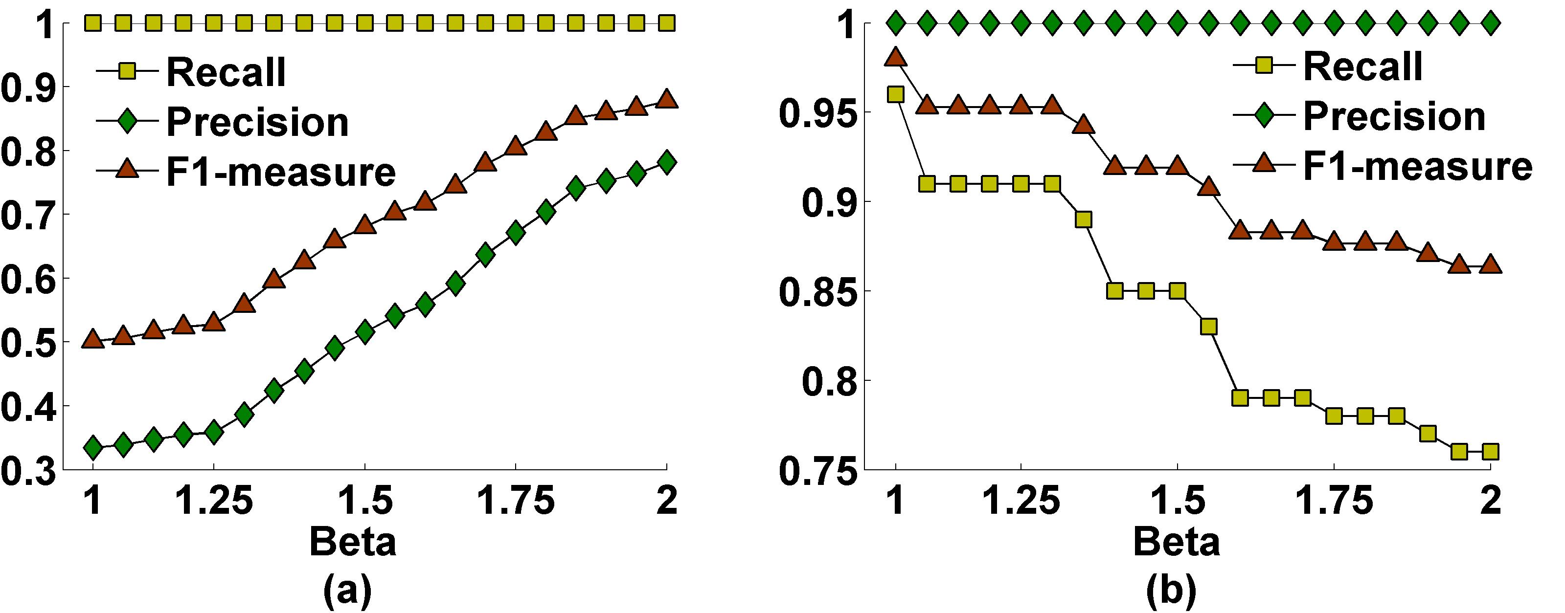
Figure 6: The variations of $Recall$,$Precision$ and $F1$-$measure$ along with $\beta$ values. (a) and (b) demonstrate the variations in $FT$ approach and $FT$-$X$ approach respectively.

Although the extended version of Shewhart control charts is capable of identifying failures adaptively, it’s still necessary to determine two parameters, namely the sliding window $N^{{}^{\prime}}$ and $\epsilon$ in order to obtain an optimal detection result. Figure 7$\sim$10 demonstrate the $Recall$, $Precision$,$F1$-$measure$ and $ATTF$ variations along with $\epsilon$ and $N^{{}^{\prime}}$ respectively. The variation zone is organized as 10x14 mesh grid. From Figure 7, we observe that in the area where $2\leq N^{{}^{\prime}}\leq 6$ and $4\leq\epsilon\leq 7$, some values are 0 (i.e. $N_{tp}=0$) as there are no deviations exceeding the threshold $\epsilon$. Accordingly, the $Precision$ and $F1$-$measure$ are 0 too. But in other areas, all the failure points are detected (i.e. $Recall=1$). Thus $F1$-$measure$ changes consistently with $Precision$. Here we choose the optimal result when $N=6$ and $\epsilon=6.5$ according to $F1$-$measure$. At this point, $Recall=1$,$Precision=0.99$, F1-measure=0.995 and $ATTF=6$.

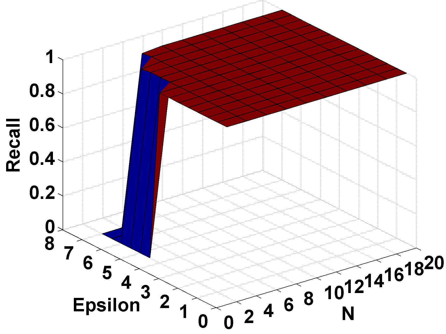
Figure 7: $Recall$ variations

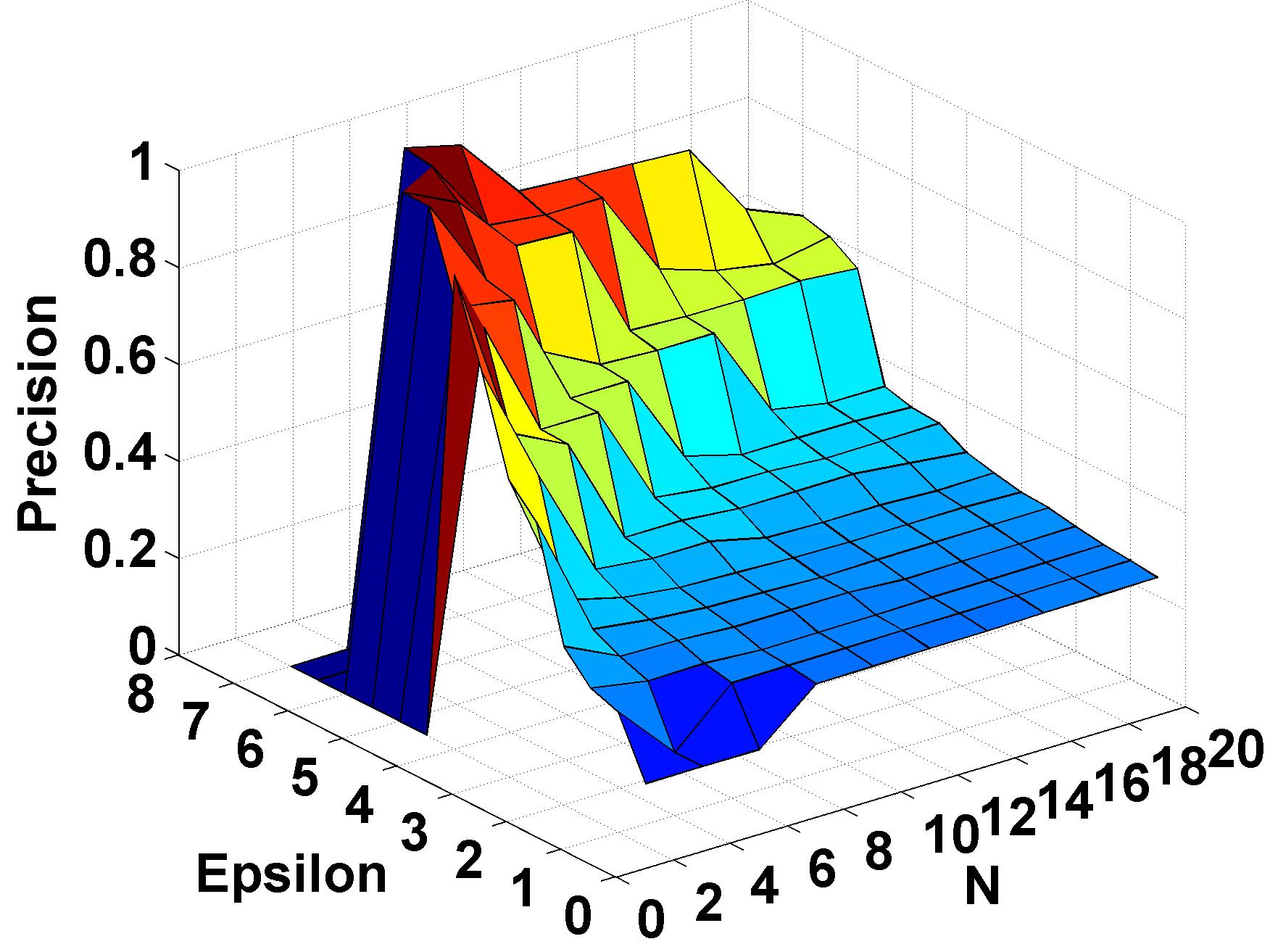
Figure 8: $Precision$ variations

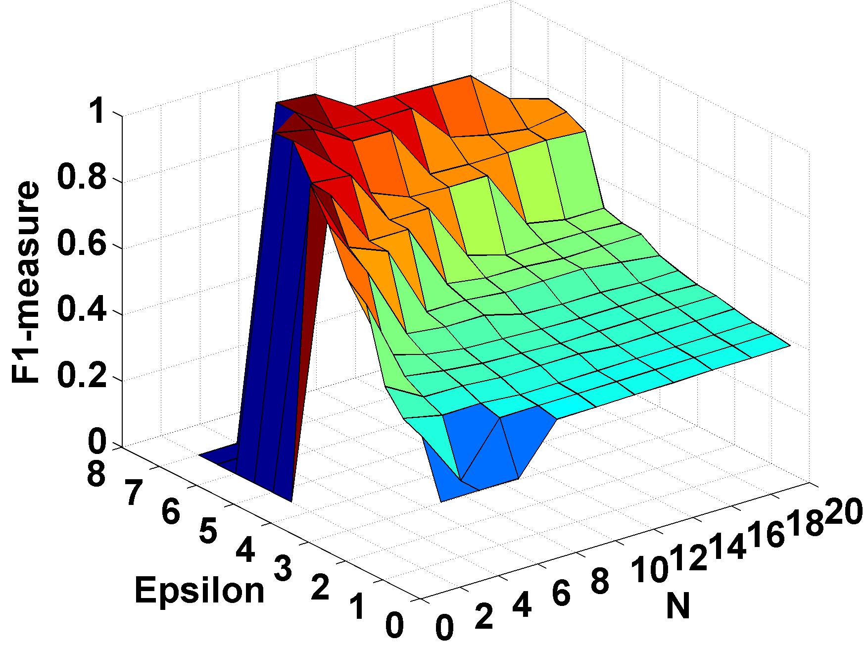
Figure 9: $F1$-$measure$ variations

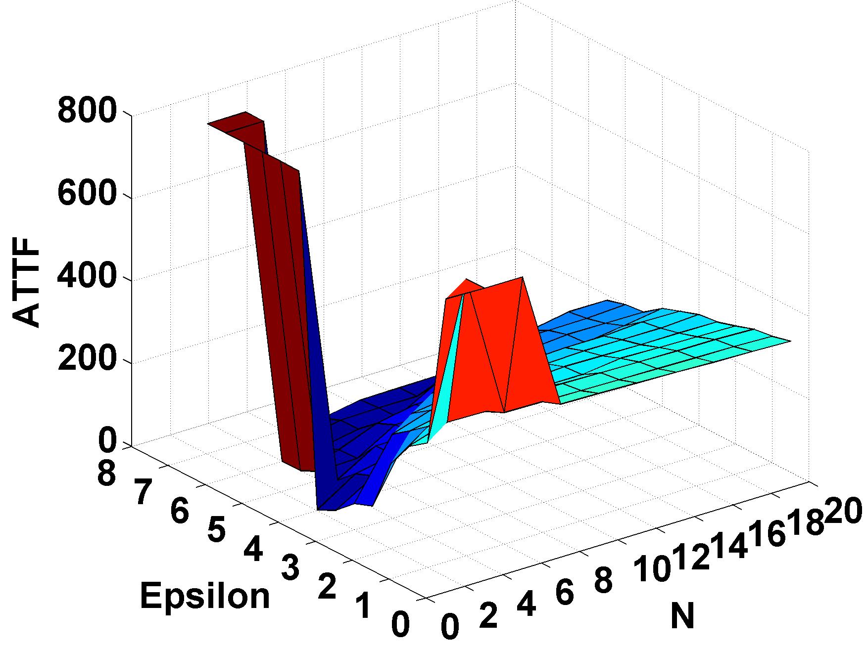
Figure 10: $ATTF$ variations

In the following experiments, we will compare the detection results of $FT$, $FT$-$X$ and the extended version of Shewhart control charts when they achieve the optimal results in the Helix Server system and the real-world AntVision system. In different systems, we will determine the optimal results for different approaches separately.

Figure 11 depicts the comparisons of the failure detection results obtained by $FT$, $FT$-$X$ and the extended Shewhart control charts in Helix Sever system. From Figure 11.(a), we observe that the extended version of Shewhart control chart achieves the best result, $F1$-$measure$=0.995; $FT$-$X$ achieves the second best result, $F1$-$measure$=0.9795; $FT$ achieves the worst result, $F1$-$measure$=0.8899. The detection results of the extended Shewhart control chart and $FT$-$X$ have about 0.1 improvement compared to the one of $FT$. Meanwhile, a lower $ATTF$ is obtained by the adaptive approaches such as $FT$-$X$, shown in Figure 11.(b). A lower $ATTF$ not only guarantees the failure could be detected in time but also reduces the excessive maintenance cost. Via these comprehensive comparisons, we find that based upon MMSE, the adaptive approaches outperform the statical approaches due to their adaptation to the ever changing runtime environment.

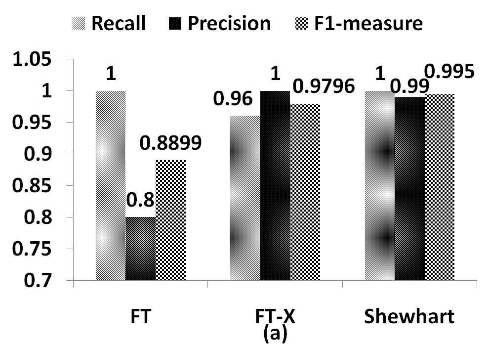
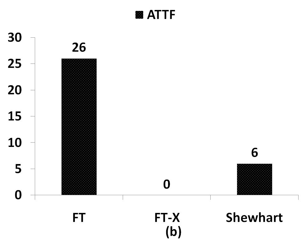
Figure 11: The comparisons of the failure detection results obtained by $FT$, $FT$-$X$ and Shewhart control charts in Helix Sever system. (a) presents $Recall$, $Precision$ and $F1$-$measure$ comparisons and (b) presents $ATTF$ comparisons.

Figure 12 shows one slice of MMSE time series in the range $1100\sim 1320$ calculated by MMSE algorithm on the performance metrics collected in AntVision system and the optimal failure reports generated by $FT$, $FT$-$X$ and Shewhart control chart. The failure reports generated by $FT$, $FT$-$X$ and Shewhart control chart fall in the range $1213\sim 1320$, $1217\sim 1320$ and $1219\sim 1320$ respectively. It is intuitively observed that Shewhart control chart approach achieves the best detection result as almost all its failure reports fall in the decision window. However the detection results achieved by $FT$ and $FT$-$X$ are very similar. This is because there are no significant changes for MMSE in the range $1000\sim 1220$, which results in the optimal threshold determined by $FT$ and $FT$-$X$ are very similar, namely 0.233 and 0.4 respectively. Figure 13 demonstrates the comparisons of failure detection results in terms of $Recall$,$Precision$, $F1$-$measure$ and $ATTF$. The results also tell us that the adaptive approach based upon MMSE indicator is capable of achieving a better detection accuracy and a lower $ATTF$. To make a broad comparison with the approaches based upon other aging indicators, we conduct the following experiments.

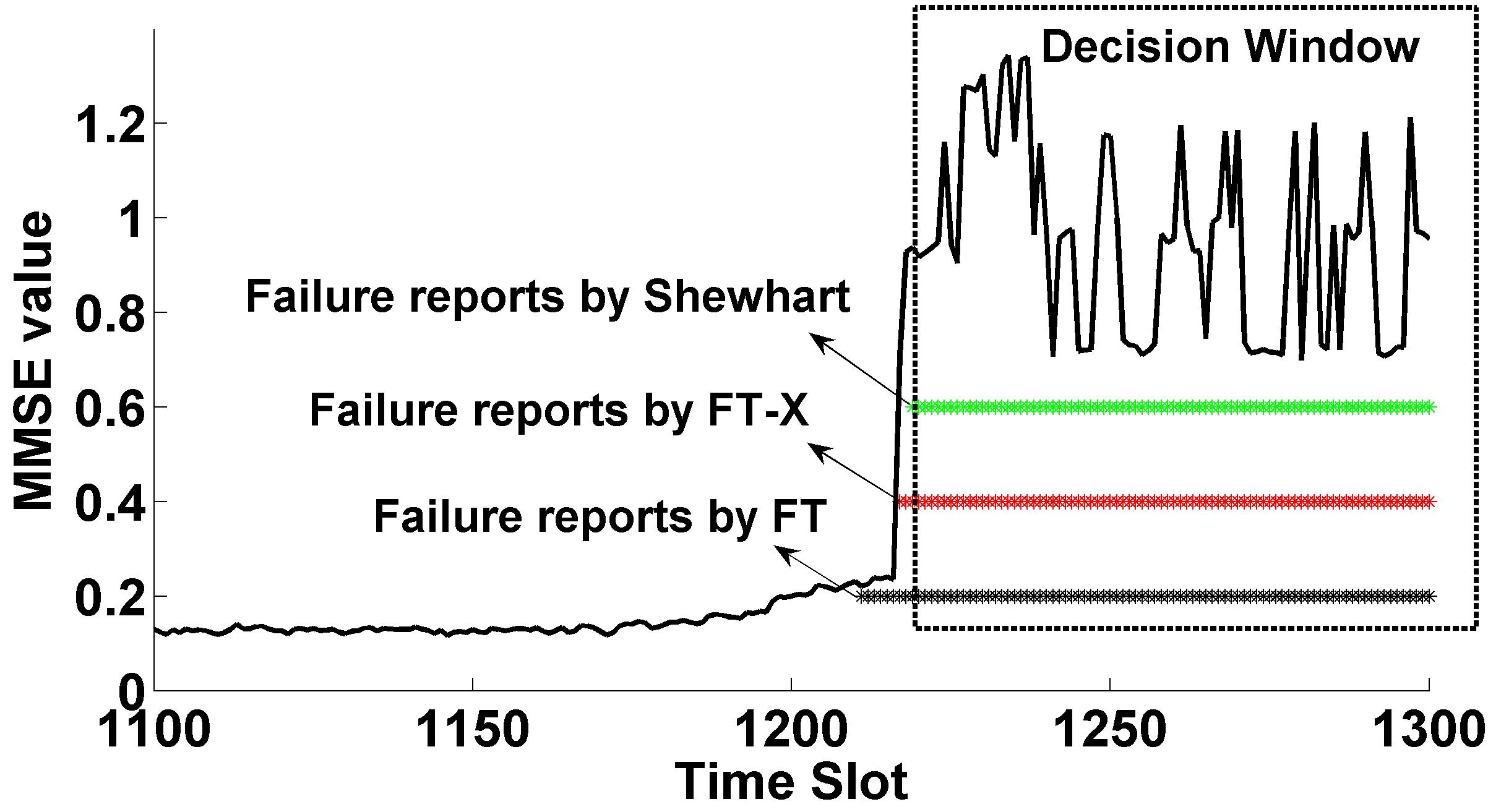
Figure 12: One slice of MMSE data and the failure reports generated by $FT$, $FT$-$X$ and Shewhart control chart in AntVision system.

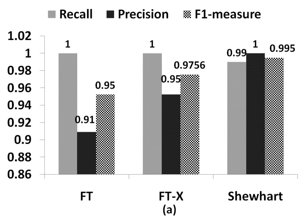
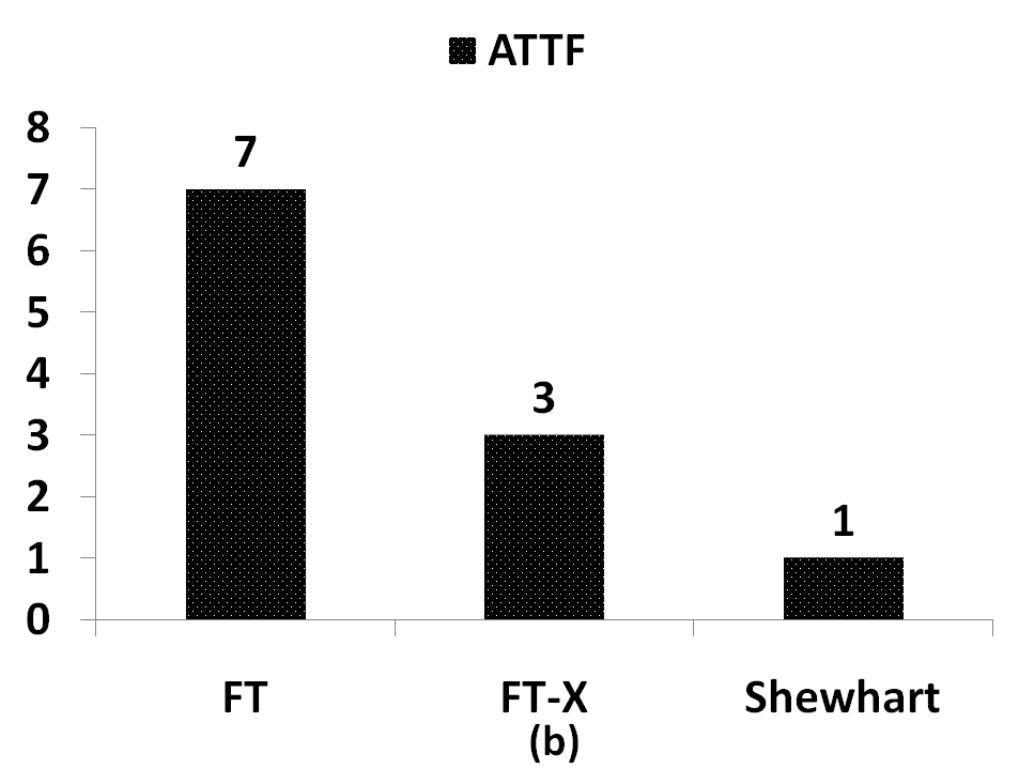
Figure 13: The comparisons of the failure detection results obtained by $FT$, $FT$-$X$ and Shewhart control charts in AntVision system.

5.4 Comparison

In this section, we will compare the failure detection results obtained by the approaches based upon MMSE and the approaches based upon other explicit or implicit indicators. In previous studies, QoS metrics (e.g. response time, throughout) or runtime performance metrics (e.g. CPU utilization) are more often than not adopted as explicit aging indicators. Accordingly, we adopt AverageBandwidth as an explicit aging indicator in Helix Server system and CPU utilization as an explicit aging indicator in AntVision system. $H\ddot{o}lder$ exponent mentioned in [19] is adopted as an implicit aging indicator in these two systems. For different aging indicators, the failure detection approaches vary a little. For AverageBandwidth and $H\ddot{o}lder$ exponent indicators, we employ a lower boundary test in the threshold based approach and the extended version of Shewhart control chart proposed in [19] in the time series approach both of which are depicted in Section V.D, due to their downtrend characteristics. It’s worth noting that $\beta$ should vary in the same range e.g. 1$\sim$20 in this paper for $FT$ and $FT$-$X$ in order to conduct fair comparisons. All of comparisons are conducted in the situations when these failure detection approaches achieve optimal results.

We first determine the optimal conditions when these approaches achieve their optimal results in Helix Server system. Table I demonstrates these optimal conditions. Figure 14 shows the comparison results for different indicators in terms of $Recall$, $Precision$, $F1$-$measure$ and $ATTF$ respectively.

TABLE I: The optimal conditions for different approaches based upon different aging indicators in Helix Server system

	FT	FT-X	Shewhart control chart
AverageBandwidth	$\beta=1.8$	$\beta=1.8$	$N^{{}^{\prime}}$=440,$\epsilon=8$
MMSE	$\beta=2$	$\beta=1.1$	$N^{{}^{\prime}}$=4,$\epsilon=6$
$H\ddot{o}lder$	$\beta=5.3$	$\beta=5.3$	$N^{{}^{\prime}}$=40,$\epsilon=5$

From Figure 14.(a), we observe that the extended version of Shewhart control chart approach achieves an ideal recall (i.e. $Recall=1$) no matter which indicator is chosen. However for $FT$ and $FT$-$X$ approaches, the detection result heavily depends on aging indicators. The $Recall$ of $FT$ and $FT$-$X$ based upon MMSE are 1 and 0.91 respectively, much higher than the results obtained by the approaches based upon AverageBandwidth, 0.52 and $H\ddot{o}lder$, 0.62. The effectiveness of MMSE is even more significant than the other two indicators in term of $Precision$. We observe that the $Precision$ of failure detection approaches based upon MMSE is up to 9 times higher than the one of $FT$ or $FT$-$X$ based upon $H\ddot{o}lder$, and 5 times higher than the one of $FT$ or $FT$-$X$ based upon AverageBandwidth, shown in Figure 14.(b). Accordingly, the MMSE is much more powerful to detect AOF than $H\ddot{o}lder$ and AverageBandwidth in $F1$-$measure$ demonstrated in Figure 14.(c). From the point of view of $ATTF$, the approaches based upon MMSE obtain up to 3 orders of magnitude improvement than the ones based upon the other two indicators. For example in Figure 14.(d), for $FT$-$X$ approach, the $ATTF$ based upon AverageBandwidth and $H\ddot{o}lder$ are 1570 and 1700 respectively, but the $ATTF$ based upon MMSE is 0. The extraordinary effectiveness of MMSE is attributed to its three properties: monotonicity, stability and integration. However, the single runtime parameter e.g. AverageBandwidth can’t comprehensively reveal the aging state of the whole system and the fluctuations involved in this indicator result in much detection bias. Figure 15 shows a representative $AverageBandwidth$ variations from system start to “failure”. We observe that the AverageBandwidth may be low even at normal state. The $H\ddot{o}lder$ exponent indicator also suffers from this problem. Although a downtrend indeed exists in $H\ddot{o}lder$ exponent indicator indicating the complexity is increasing which is compliant with the result in [19], shown in Figure 16, the instability hinders to achieve a high accurate failure detection result. From above comparisons, we find out the detection results obtained by $FT$ and $FT$-$X$ based upon $AverageBandwidth$ or $H\ddot{o}lder$ are the same. That’s because the minimum point of the aging indicator is involved simultaneously in the training data of $FT$ and $FT$-$X$ demonstrated in Figure 15 and Figure 16. Therefore the optimal threshold values calculated by $FT$ and $FT$-$X$ are the same.

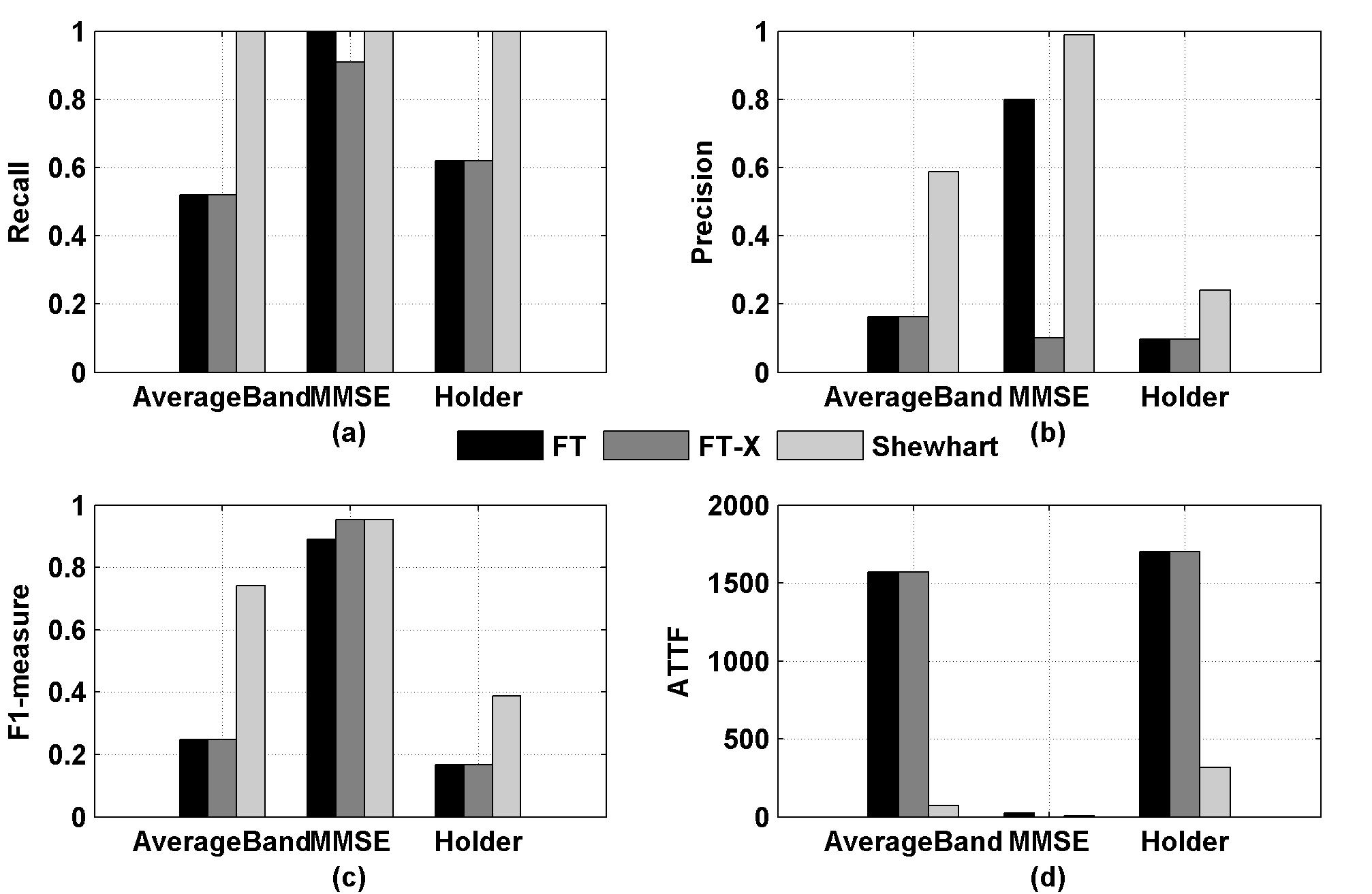
Figure 14: The comparison results of the detection approaches based upon different aging indicators in Helix Server system. Here “AB” is short for AverageBandwidth.

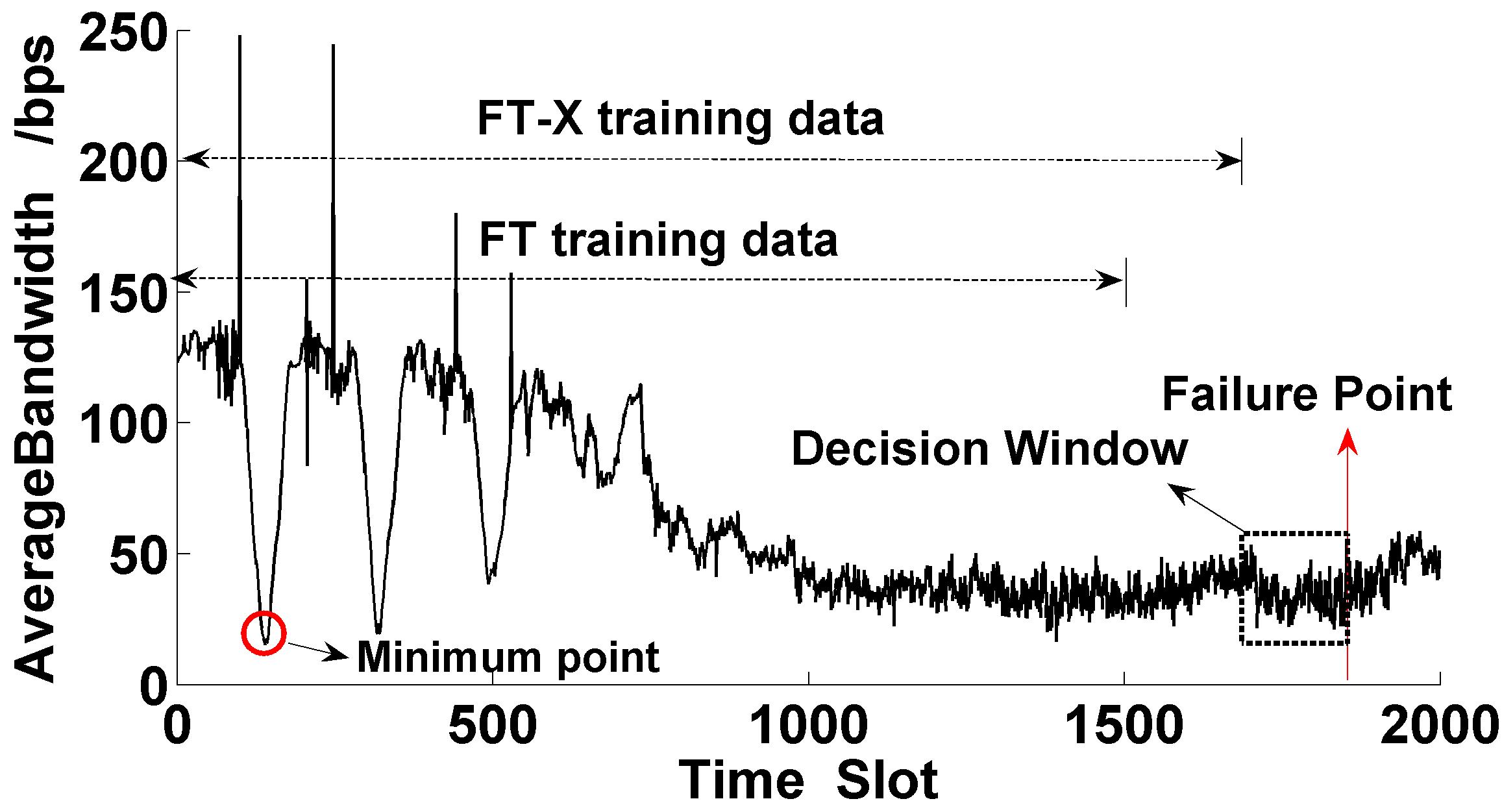
Figure 15: The AverageBandwidth data from system start to “failure”.

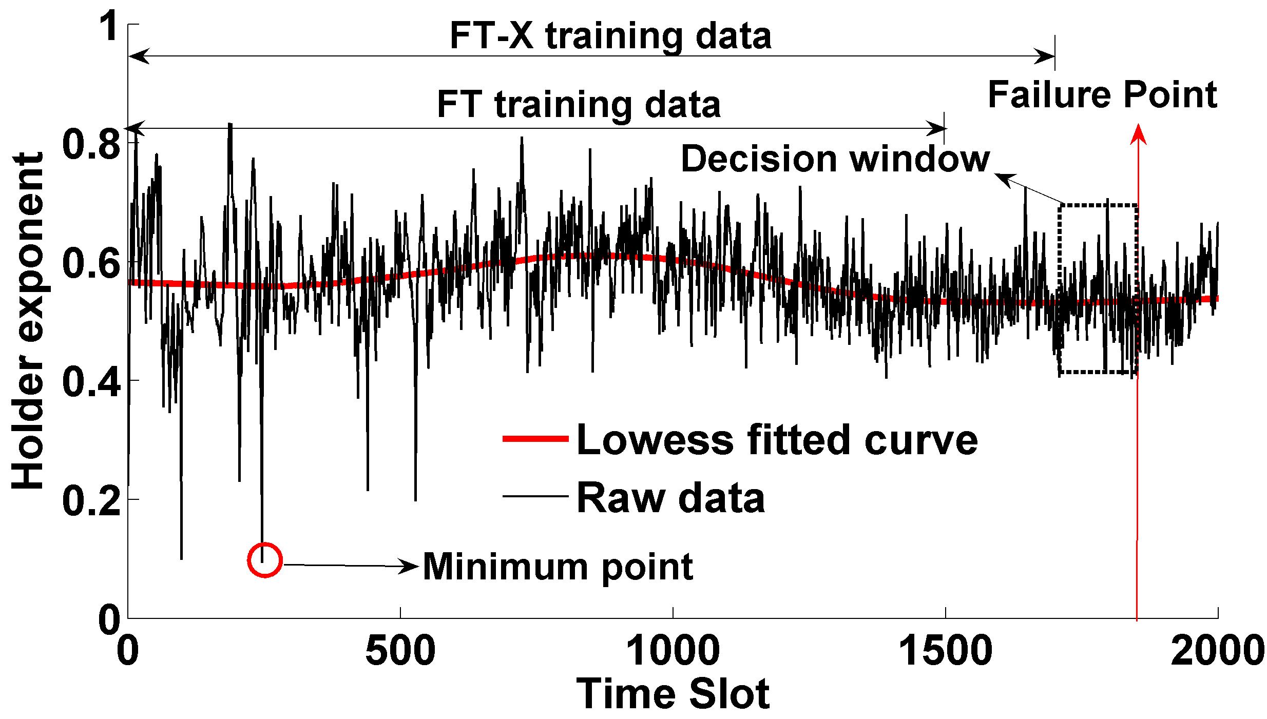
Figure 16: The $H\ddot{o}lder$ data from system start to “failure”. The curve fitted by $Lowess$ [36] is used to present the downtrend.

The optimal conditions for these failure detection approaches based upon CPU Utilization, MMSE and $H\ddot{o}lder$ exponent in AntVision system are listed in Table II.

TABLE II: The optimal conditions for different approaches based upon different aging indicators in AntVision system

	FT	FT-X	Shewhart control chart
CPU Utilization	$\beta=1$	$\beta=-$	$N^{{}^{\prime}}$=75,$\epsilon=17$
MMSE	$\beta=2$	$\beta=1.3$	$N^{{}^{\prime}}$=8,$\epsilon=7$
$H\ddot{o}lder$	$\beta=4.0$	$\beta=19$	$N^{{}^{\prime}}$=165,$\epsilon=8$

An interesting finding is that the optimal condition of $FT$-$X$ based upon CPU Utilization indicator is $\beta=-$ which means we can’t find an optimal $\beta$ in the range $1\sim 20$. By investigating the detection results, we observe that the $Recall$, $Precision$ and $F1$-$measure$ are all 0 no matter which value $\beta$ is chosen in the range $1\sim 20$. Figure 17 provides the reason why we get this observation. The maximum CPU utilization involved in the training data in $FT$-$X$ falling in the range $1\sim 1200$, exceeds all the CPU Utilization in the decision window. Therefore according to the threshold calculated by $FT$-$X$, we can’t detect any failures (i.e. $N_{tp}=0$). While for $FT$ approach, the maximum CPU utilization in the training data is lower than the maximum CPU Utilization in the decision window. Hence some failure points can be detected by $FT$. This is the reason why $FT$ outperforms $FT$-$X$ based upon CPU Utilization in AntVision system. And this could be regarded as a drawback of non-monotonicity of the CPU Utilization indicator.

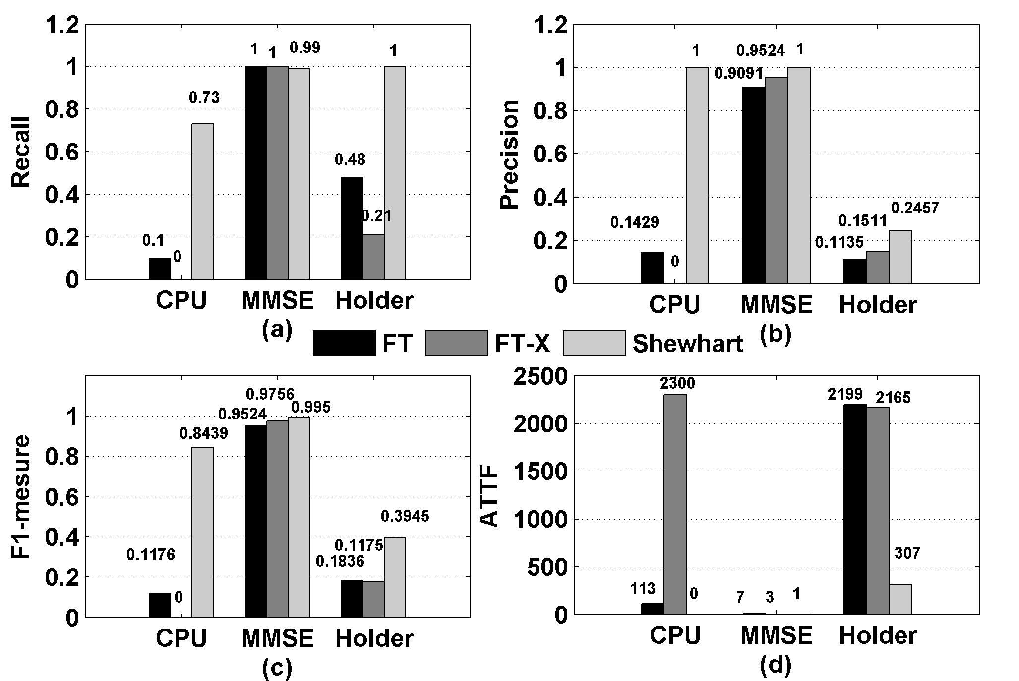
Figure 17: The CPU utilization and corresponding MMSE data in AntVision system.

Figure 18 demonstrates the comparison results in terms of $Recall$,$Precision$,$F1$-$measure$ and $ATTF$ amongst the failure detection approaches based upon different aging indicators in AntVision system. From this figure, we observe that the $F1$-$measure$ achieved by MMSE-based approaches are higher than 0.95 and much better than the one achieved by CPU Utilization-based and $H\ddot{o}lder$ exponent-based approaches. Meanwhile, the $ATTF$ is significantly reduced from a large number (e.g. 2300) to a very tiny number (e.g. 1) by MMSE-based approaches. We also observe that the extended version of Shewhart control chart approach performs better than the other two approaches no matter which indicator is chosen.

Finally, through comprehensive comparisons above, we conclude that MMSE-based approaches extraordinarily outperform an explicit indicator (i.e. CPU Utilization) based approach and an implicit indicator (i.e. $H\ddot{o}lder$ exponent) based approach. The high accuracy of MMSE results from its three properties: Monotonicity,Stability,Integration. And based upon MMSE, the adaptive detection approaches i.e. the extended version of Shewhart control chart performs better.

Figure 18: The comparison results of the detection approaches based upon different aging indicators in AntVision system. Here “CPU” means CPU utilization.

5.5 Overhead

The whole analysis procedure of CHAOS except data collection is conducted on a separate machine. Hence it causes very little resource footprint on a test or production system. To evaluate whether CHAOS satisfies the realtime requirement, we calculate the execution time of the whole procedure. The average execution time of different modules of CHAOS in AntVision system are shown in table III where MS means Metric selection, MMSE-C means MMSE calculation. Even the most computation-intensive module, namely Metric selection module only consumes 0.875 second and the whole procedure consumes a little more than 1 second. Therefore CHAOS is light-weight enough to satisfy the realtime requirement.

TABLE III: The average execution time of different modules of CHAOS in AntVision system.

	MS	MMSE-C	FT	FT-X	Shewhart
Time (second)	0.875	0.123	0.016	0.018	0.270

6 Related work

As the first line of defending software aging, accurate detection of Aging-Oriented Failure is essential. A large quantity of work has been done in this area. Here we briefly discuss related work that has inspired and informed our design, especially work not previously discussed. The related work could be roughly classified into two categories: explicit indicator based method and implicit indicator based method.

Explicit indicator based method: The explicit indicator based method usually uses the directly observed performance metrics as the aging indicators and develops aging detection approaches based upon these indicators. Actually according to our review, most of prior studies such as [2, 3, 4, 5, 8, 9, 12, 13, 14, 17, 18, 39, 40] and etc belong to this class. In [3, 8, 17, 18], they treat system resource usage (e.g. CPU or memory utilization,swap space) as the aging indicator while [4, 5, 12, 13, 14, 40] take the application specific parameters (e.g. response time, function call) as the aging indicators. Based on these indicators, they detect or predict Aging-Oriented Failure via time-series analysis [4, 9, 12, 17, 18], machine learning [5, 41, 39] or threshold-based approach [33, 34]. The common drawback of these approaches is embodied in the aging indicators’ insufficiency due to their weak correlation with software aging. Hence the detection or prediction results have not reached a satisfactory level no matter which approaches are adopted. Against this drawback, this paper proposes a new aging indicator,MMSE, which is extracted from the directly observed performance metrics.

Implicit indicator based method: Contrary to the explicit indicator based method, the implicit indicator based method employs aging indicators embedded in the directly observed performance metrics. These aging indicators are declared to be more sufficient to indicate software aging. Our method falls into this class. Cassidy, et.al [31] and Gross, et.al [27] leveraged “residual” between the actual performance data (e.g. queue length) and the estimated performance data obtained by a multivariate analysis method (e.g. Multivariate State Estimation Technique) as the aging indicator. Then the software’s fault detection procedure used a Sequential Probability Ratio Test (SPRT) technique to determine whether the residual value is out of bound. Mark, et.al [19] proposed another implicit aging indicator: $H\ddot{o}lder$ exponent. They showed that the $H\ddot{o}lder$ exponent of memory utilization decreased with the degree of software aging. By identifying the second breakdown of $H\ddot{o}lder$ exponent data series through an online Shewhart algorithm, the Aging-Oriented Failure was detected. Although Jia [14] didn’t introduce any implicit aging indicator, he showed software aging process was nonlinear and chaotic. Hence, some complexity-related metrics such as entropy, Lyapunov exponent and etc are possible to be aging indicators. And our work is inspired by Mark , et.al [19] and Jia, et.al [14]. However, the prior studies had no quantitative proof about the viability of their implicit aging indicators, no abstraction of the properties that an ideal aging indicator should have and no multi-scale extension. Moreover the effectiveness of $H\ddot{o}lder$ exponent was only evaluated under emulated increasing workload and a thorough evaluation under real workload was absent in the their paper. These defects will result in bias in the detection results, which is shown in the real experiments in section VI.

Another implicit indicator is MSE, although it hasn’t been employed in software aging analysis before this work. However MSE has been widely used to measure the irregularity variation of pathological data such as electrocardiogram data [32, 25, 28, 42]. Motivated by these studies, we first introduce MSE to software aging area. However, we argue that software aging is a complex procedure affected by many factors. Hence,to accurate measure software aging, a multi-dimensional approach is necessary. We extend the conventional MSE to MMSE via several modifications. Wang, et.al [43] also adopts entropy as an indicator of performance anomaly. But he measures the entropy using the traditional Shannon entropy rather than MSE.

7 Conclusion

In this paper, we proposed a novel implicit aging indicator namely MMSE which leverages the complexity embedded in runtime performance metrics to indicate software aging. Through theoretical proof and experimental practice, we demonstrate that entropy increases with the degree of software aging monotonously. To counteract the system fluctuations and comprehensively describe software aging process, MMSE integrates the entropy values extracted from multi-dimensional performance metrics at multiple scales. Therefore, MMSE satisfies the three properties, namely Monotonicity, Stability, and Integration which we conjecture an ideal aging indicator should have. Based upon MMSE, we design and develop a proof-of-concept named CHAOS which contains three failure detection approaches, namely $FT$ and $FT$-$X$ and the extended version of Shewhart control chart. The experimental evaluation results in a VoD system and in a real-world production system, AntVision, show that CHAOS can achieve extraordinarily high accuracy and near 0 $ATTF$. Due to the Monotonicity of MMSE, the adaptive approaches such as $FT$-$X$ outperform the static approach such as $FT$ while this is not true for other aging indicators. Compared to previous approaches, the accuracy of failure detection approaches based upon MMSE is increased by up to 5 times, and the $ATTF$ is reduced by 3 orders of magnitude. In addition, CHAOS is light-weight enough to satisfy the realtime requirement. We believe that CHAOS is an indispensable complement to conventional failure detection approaches.

Appendix A Proof of Entropy Increase

Our proof is based on three basic assumptions:
Assumption 1: The software systems or components only exhibit binary states during running: working state $s_{w}$ and failure state $s_{f}$.
Assumption 2: The probability of $s_{f}$ increases monotonously with the degree of software aging.
Assumption 3: If the probability of $s_{w}$ is less than the probability of $s_{f}$ , the system will be rejuvenated at once.

A system or a component may exhibit more than two states during running, but here we only consider two states: working and failure state, which is compliant with the classical three states i.e. up ,down and rejuvenation mentioned in [7, 44, 45] without considering rejuvenation state. According to the description of software aging stated in the introduction section, the failure rate increases with the degree of software aging. Thus Assumption 2 is intuitional. Actually increasing failure probability is also a common assumption in previous studies [46, 47, 48, 49, 44, 45] in order to obtain an optimal rejuvenation scheduling. For a software system, it’s unacceptable if only a half or even less of the total requests are processed successfully especially in modern service oriented systems. A software system is forced to restart before it enters into a non-service state. Therefore Assumption 3 is reasonable.

If the software system is represented as a single component, the system entropy at time $t$ is defined as:

$$E(t)=-(p_{w}(t)*ln(p_{w}(t))+p_{f}(t)*ln(p_{f}(t)))$$ (9)

where $p_{w}(t)$ and $p_{f}(t)$ represent the probability of normal state $s_{w}$ and failure state $s_{f}$ at time $t$ respectively and $p_{w}(t)+p_{f}(t)=1$. At the initial stage, namely $t=0,p_{w}(0)=1$, we say the system is completely new. At this moment, the entropy $E(t)$ equals 0. As software performance degradation, $p_{w}(t)$ decreases from 1 to 0 while $p_{f}(t)$ increases from 0 to 1. We assume the failure rate $h(t)$ conforms to a Weibull distribution with two parameters which is commonly used in previous studies [50, 47, 44, 45]. The distribution is described as:

$$h(t)=\frac{\beta}{\alpha}({\frac{t}{\alpha}})^{\beta-1}{e}^{-({\frac{t}{\alpha}})^{\beta}}$$ (10)

where $\beta$ denotes the shape parameter and $\alpha$ denotes the scale parameter. Because

$$h(t)=\frac{dF(t)/dt}{1-F(t)}=\frac{p_{f}(t)}{1-F(t)}$$ (11)

where $F(t)$ denotes the cumulative distribution function (CDF) of $p_{f}(t)$. And

$$F(t)=1-{e}^{\int_{0}^{t}h(t)dt}=1-e^{-(\frac{t}{\alpha})^{\beta}}$$ (12)

Therefore $p_{f}(t)$ could be expressed as:

$$p_{f}(t)=\frac{\beta}{\alpha}({\frac{t}{\alpha}})^{\beta-1}{e}^{-2({\frac{t}{\alpha}})^{\beta}}$$ (13)

In [44], they determined $\alpha$ and $\beta$ via parameter estimation and gave a confidence range for $\alpha$ and $\beta$ respectively. Based upon their result, we set $\alpha=5.4E5$ and $\beta=11$ in this paper. The failure probability, $p_{f}(t)$, from time 0 to time $4.5E5$ (system crash assumed) is depicted in Figure 19. Accordingly the entropy, $E(t)$, is demonstrated in Figure 20. From Figure 20, we observe that entropy increases monotonously during the life time of the running system. In this case, the failure probability curve is truncated at system crash, far from the point where $p_{f}(t)=p_{w}(t)$. In some corner cases, $p_{f}(t)$ can reach the point where $p_{f}(t)=p_{w}(t)$. However, the system suffers from SLA violations and restarts very soon when $p_{f}(t)>p_{w}(t)$. Thus we only take into account the scenario when $p_{f}(t)<p_{w}(t)$. In this scenario, the system entropy increases monotonously. Therefore Theorem 1 is true as long as $p_{f}(t)$ or $p_{w}(t)$ varies monotonously.

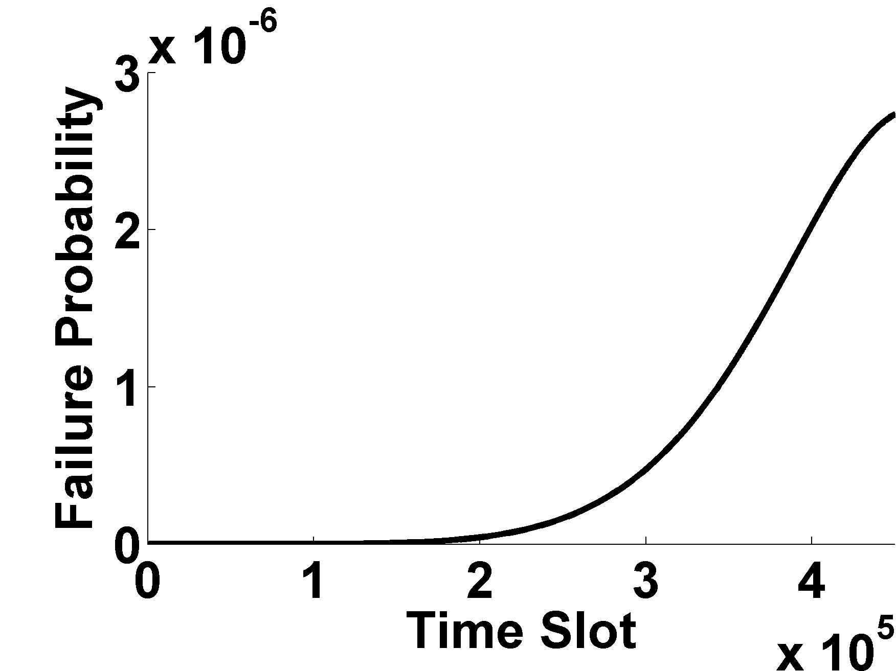
Figure 19: $p_{f}(t)$ variation curve

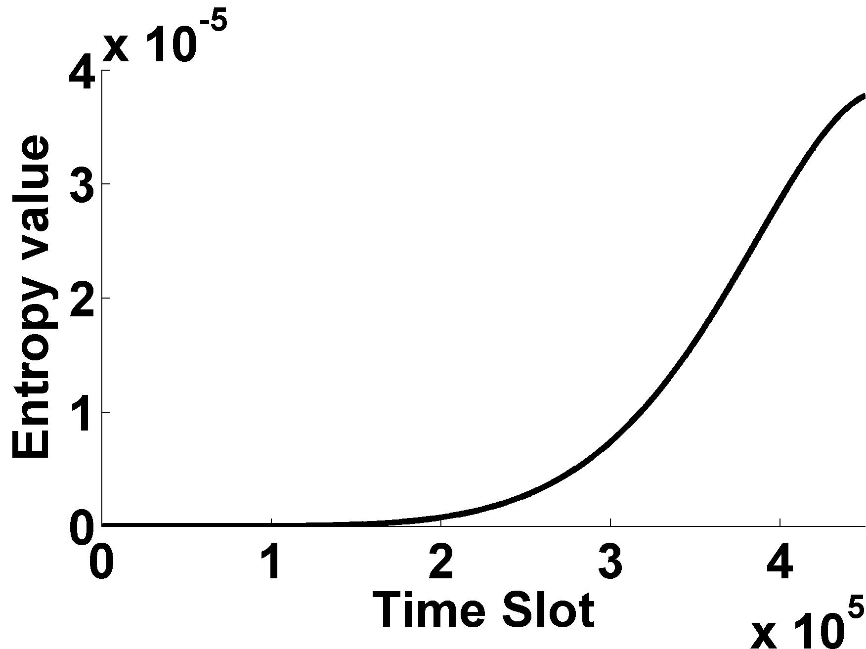
Figure 20: $E(t)$ variation curve

Theorem 1.

If $p_{f}(t)$ increases monotonously, the system entropy $E(t)$ monotonously increases with the degree of software aging when $p_{f}(t)<p_{w}(t)$ or $p_{f}(t)<\frac{1}{2}$

Proof.

When $p_{f}(t)=0$ or $p_{f}(t)=1$, $ln(1-p_{f}(t))$ or $ln(p_{f}(t))$ is not defined. Hence we assume $p_{f}(t)\in(0,1)$. Substitute $p_{w}(t)$ with $1-p_{f}(t)$ in equation (12). Then we get:

$$E(t)=-((1-p_{f}(t))*ln(1-p_{f}(t))+p_{f}(t)*ln(p_{f}(t)))$$

$$\quad\quad=-ln(1-p_{f}(t))+p_{f}(t)*(ln(1-p_{f}(t))-ln(p_{f}(t)))$$

Regard $p_{f}(t)$ as an variable, the first order derivative and second order derivative of $E(t)$ are: $E(t)^{{}^{\prime}}=ln(1-p_{f}(t))-ln(p_{f}(t))$, $E(t)^{{}^{\prime\prime}}=-((1-p_{f}(t))*p_{f}(t))^{-1}$. As $p_{f}(t)\in(0,1)$, $E(t)^{{}^{\prime\prime}}<0$. Therefore $E(t)$ achieves the maximum value when $E(t)^{{}^{\prime}}=0$ namely $ln(p_{f}(t))=ln(1-p_{f}(t))$ Finally, we get $p_{f}(t)=\frac{1}{2}$. As $p_{f}(t)$ increases monotonously, $E(t)$ increases monotonously when $p_{f}(t)<\frac{1}{2}$. Hence Theorem 1 is proved. ∎

References

- [1] K. Vaidyanathan and K. S. Trivedi, “A measurement-based model for estimation of resource exhaustion in operational software systems,” in Software Reliability Engineering, 1999. Proceedings. 10th International Symposium on. IEEE, 1999, pp. 84–93.
- [2] K. Vaidyanathan, R. E. Harper, S. W. Hunter, and K. S. Trivedi, “Analysis and implementation of software rejuvenation in cluster systems,” in ACM SIGMETRICS Performance Evaluation Review, vol. 29, no. 1. ACM, 2001, pp. 62–71.
- [3] K. Vaidyanathan and K. S. Trivedi, “A comprehensive model for software rejuvenation,” Dependable and Secure Computing, IEEE Transactions on, vol. 2, no. 2, pp. 124–137, 2005.
- [4] M. Grottke, L. Li, K. Vaidyanathan, and K. S. Trivedi, “Analysis of software aging in a web server,” Reliability, IEEE Transactions on, vol. 55, no. 3, pp. 411–420, 2006.
- [5] J. Alonso, J. Torres, J. L. Berral, and R. Gavalda, “Adaptive on-line software aging prediction based on machine learning,” in Dependable Systems and Networks (DSN), 2010 IEEE/IFIP International Conference on. IEEE, 2010, pp. 507–516.
- [6] S. P. Kavulya, S. Daniels, K. Joshi, M. Hiltunen, R. Gandhi, and P. Narasimhan, “Draco: Statistical diagnosis of chronic problems in large distributed systems,” in Dependable Systems and Networks (DSN), 2012 42nd Annual IEEE/IFIP International Conference on. IEEE, 2012, pp. 1–12.
- [7] Y. Huang, C. Kintala, N. Kolettis, and N. D. Fulton, “Software rejuvenation: Analysis, module and applications,” in Fault-Tolerant Computing, 1995. FTCS-25. Digest of Papers., Twenty-Fifth International Symposium on. IEEE, 1995, pp. 381–390.
- [8] J. Araujo, R. Matos, V. Alves, P. Maciel, F. Souza, K. S. Trivedi et al., “Software aging in the eucalyptus cloud computing infrastructure: Characterization and rejuvenation,” ACM Journal on Emerging Technologies in Computing Systems (JETC), vol. 10, no. 1, p. 11, 2014.
- [9] J. Araujo, R. Matos, P. Maciel, R. Matias, and I. Beicker, “Experimental evaluation of software aging effects on the eucalyptus cloud computing infrastructure,” in Proceedings of the Middleware 2011 Industry Track Workshop. ACM, 2011, p. 4.
- [10] K. Kourai and S. Chiba, “Fast software rejuvenation of virtual machine monitors,” Dependable and Secure Computing, IEEE Transactions on, vol. 8, no. 6, pp. 839–851, 2011.
- [11] ——, “A fast rejuvenation technique for server consolidation with virtual machines,” in Dependable Systems and Networks, 2007. DSN’07. 37th Annual IEEE/IFIP International Conference on. IEEE, 2007, pp. 245–255.
- [12] D. Cotroneo, R. Natella, R. Pietrantuono, and S. Russo, “Software aging analysis of the linux operating system,” in Software Reliability Engineering (ISSRE), 2010 IEEE 21st International Symposium on. IEEE, 2010, pp. 71–80.
- [13] D. Cotroneo, S. Orlando, and S. Russo, “Characterizing aging phenomena of the java virtual machine,” in Reliable Distributed Systems, 2007. SRDS 2007. 26th IEEE International Symposium on. IEEE, 2007, pp. 127–136.
- [14] Y.-F. Jia, L. Zhao, and K.-Y. Cai, “A nonlinear approach to modeling of software aging in a web server,” in Software Engineering Conference, 2008. APSEC’08. 15th Asia-Pacific. IEEE, 2008, pp. 77–84.
- [15] B. Sharma, P. Jayachandran, A. Verma, and C. R. Das, “Cloudpd: Problem determination and diagnosis in shared dynamic clouds,” in IEEE DSN, 2013.
- [16] V. Castelli, R. E. Harper, P. Heidelberger, S. W. Hunter, K. S. Trivedi, K. Vaidyanathan, and W. P. Zeggert, “Proactive management of software aging,” IBM Journal of Research and Development, vol. 45, no. 2, pp. 311–332, 2001.
- [17] P. Zheng, Y. Qi, Y. Zhou, P. Chen, J. Zhan, and M. Lyu, “An automatic framework for detecting and characterizing performance degradation of software systems,” Reliability, IEEE Transactions on, vol. 63, no. 4, pp. 927–943, 2014.
- [18] S. Garg, A. van Moorsel, K. Vaidyanathan, and K. S. Trivedi, “A methodology for detection and estimation of software aging,” in Software Reliability Engineering, 1998. Proceedings. The Ninth International Symposium on. IEEE, 1998, pp. 283–292.
- [19] M. Shereshevsky, J. Crowell, B. Cukic, V. Gandikota, and Y. Liu, “Software aging and multifractality of memory resources,” in 2003 33rd Annual IEEE/IFIP International Conference on Dependable Systems and Networks (DSN). IEEE Computer Society, 2003, pp. 721–730.
- [20] I. Jolliffe, Principal component analysis. Wiley Online Library, 2005.
- [21] J. F. Cadima and I. T. Jolliffe, “Variable selection and the interpretation of principal subspaces,” Journal of agricultural, biological, and environmental statistics, vol. 6, no. 1, pp. 62–79, 2001.
- [22] J. Ramsay, J. ten Berge, and G. Styan, “Matrix correlation,” Psychometrika, vol. 49, no. 3, pp. 403–423, 1984.
- [23] J. Cadima, J. O. Cerdeira, and M. Minhoto, “Computational aspects of algorithms for variable selection in the context of principal components,” Computational statistics & data analysis, vol. 47, no. 2, pp. 225–236, 2004.
- [24] C. E. Shannon, “Bell system tech. j. 27 (1948) 379; ce shannon,” Bell System Tech. J, vol. 27, p. 623, 1948.
- [25] M. Costa, A. L. Goldberger, and C.-K. Peng, “Multiscale entropy analysis of biological signals,” Physical Review E, vol. 71, no. 2, p. 021906, 2005.
- [26] S. M. Pincus and A. L. Goldberger, “Physiological time-series analysis: what does regularity quantify?” American Journal of Physiology, vol. 266, pp. H1643–H1643, 1994.
- [27] K. C. Gross, V. Bhardwaj, and R. Bickford, “Proactive detection of software aging mechanisms in performance critical computers,” in Software Engineering Workshop, 2002. Proceedings. 27th Annual NASA Goddard/IEEE. IEEE, 2002, pp. 17–23.
- [28] M. U. Ahmed and D. P. Mandic, “Multivariate multiscale entropy: A tool for complexity analysis of multichannel data,” Physical Review E, vol. 84, no. 6, p. 061918, 2011.
- [29] L. Cao, A. Mees, and K. Judd, “Dynamics from multivariate time series,” Physica D: Nonlinear Phenomena, vol. 121, no. 1, pp. 75–88, 1998.
- [30] D. Cotroneo, R. Natella, R. Pietrantuono, and S. Russo, “A survey of software aging and rejuvenation studies,” ACM Journal on Emerging Technologies in Computing Systems (JETC), vol. 10, no. 1, p. 8, 2014.
- [31] K. J. Cassidy, K. C. Gross, and A. Malekpour, “Advanced pattern recognition for detection of complex software aging phenomena in online transaction processing servers,” in Dependable Systems and Networks, 2002. DSN 2002. Proceedings. International Conference on. IEEE, 2002, pp. 478–482.
- [32] M. Costa, A. L. Goldberger, and C.-K. Peng, “Multiscale entropy analysis of complex physiologic time series,” Physical review letters, vol. 89, no. 6, p. 068102, 2002.
- [33] L. M. Silva, J. Alonso, and J. Torres, “Using virtualization to improve software rejuvenation,” IEEE Transactions on Computers, vol. 58, no. 11, pp. 1525–1538, 2009.
- [34] J. Alonso, Í. Goiri, J. Guitart, R. Gavalda, and J. Torres, “Optimal resource allocation in a virtualized software aging platform with software rejuvenation,” in Software Reliability Engineering (ISSRE), 2011 IEEE 22nd International Symposium on. IEEE, 2011, pp. 250–259.
- [35] [Online]. Available: http://www.sourceforge.net/projects/hyperic-hq
- [36] P. Chen, Y. Qi, P. Zheng, J. Zhan, and Y. Wu, “Multi-scale entropy: One metric of software aging,” in Service Oriented System Engineering (SOSE), 2013 IEEE 7th International Symposium on. IEEE, 2013, pp. 162–169.
- [37] P. Zheng, Y. Zhou, M. R. Lyu, and Y. Qi, “Granger causality-aware prediction and diagnosis of software degradation,” in Services Computing (SCC), 2014 IEEE International Conference on. IEEE, 2014, pp. 528–535.
- [38] [Online]. Available: http://www.helix-server.helixcommunity.org/
- [39] A. Andrzejak and L. Silva, “Using machine learning for non-intrusive modeling and prediction of software aging,” in Network Operations and Management Symposium, 2008. NOMS 2008. IEEE. IEEE, 2008, pp. 25–32.
- [40] R. Matias, P. A. Barbetta, K. S. Trivedi et al., “Accelerated degradation tests applied to software aging experiments,” Reliability, IEEE Transactions on, vol. 59, no. 1, pp. 102–114, 2010.
- [41] J. P. Magalhaes and L. Moura Silva, “Prediction of performance anomalies in web-applications based-on software aging scenarios,” in Software Aging and Rejuvenation (WoSAR), 2010 IEEE Second International Workshop on. IEEE, 2010, pp. 1–7.
- [42] M. U. Ahmed and D. P. Mandic, “Multivariate multiscale entropy analysis,” Signal Processing Letters, IEEE, vol. 19, no. 2, pp. 91–94, 2012.
- [43] C. Wang, V. Talwar, K. Schwan, and P. Ranganathan, “Online detection of utility cloud anomalies using metric distributions,” in Network Operations and Management Symposium (NOMS), 2010 IEEE. IEEE, 2010, pp. 96–103.
- [44] J. Zhao, Y. Jin, K. S. Trivedi, and R. Matias, “Injecting memory leaks to accelerate software failures,” in Software Reliability Engineering (ISSRE), 2011 IEEE 22nd International Symposium on. IEEE, 2011, pp. 260–269.
- [45] K. S. Trivedi, K. Vaidyanathan, and K. Goseva-Popstojanova, “Modeling and analysis of software aging and rejuvenation,” in Simulation Symposium, 2000.(SS 2000) Proceedings. 33rd Annual. IEEE, 2000, pp. 270–279.
- [46] A. Bobbio, M. Sereno, and C. Anglano, “Fine grained software degradation models for optimal rejuvenation policies,” Performance Evaluation, vol. 46, no. 1, pp. 45–62, 2001.
- [47] Y. Bao, X. Sun, and K. S. Trivedi, “A workload-based analysis of software aging, and rejuvenation,” Reliability, IEEE Transactions on, vol. 54, no. 3, pp. 541–548, 2005.
- [48] T. Dohi, K. Goseva-Popstojanova, and K. S. Trivedi, “Analysis of software cost models with rejuvenation,” in High Assurance Systems Engineering, 2000, Fifth IEEE International Symposim on. HASE 2000. IEEE, 2000, pp. 25–34.
- [49] R. E. Barlow and R. A. Campo, “Total time on test processes and applications to failure data analysis.” DTIC Document, Tech. Rep., 1975.
- [50] T. Dohi, K. Goseva-Popstojanova, and K. S. Trivedi, “Statistical non-parametric algorithms to estimate the optimal software rejuvenation schedule,” in Dependable Computing, 2000. Proceedings. 2000 Pacific Rim International Symposium on. IEEE, 2000, pp. 77–84.