Evaluating epoetin dosing strategies using observational longitudinal data

Abstract

Epoetin is commonly used to treat anemia in chronic kidney disease and End Stage Renal Disease subjects undergoing dialysis, however, there is considerable uncertainty about what level of hemoglobin or hematocrit should be targeted in these subjects. In order to address this question, we treat epoetin dosing guidelines as a type of dynamic treatment regimen. Specifically, we present a methodology for comparing the effects of alternative treatment regimens on survival using observational data. In randomized trials patients can be assigned to follow a specific management guideline, but in observational studies subjects can have treatment paths that appear to be adherent to multiple regimens at the same time. We present a cloning strategy in which each subject contributes follow-up data to each treatment regimen to which they are continuously adherent and artificially censored at first nonadherence. We detail an inverse probability weighted log-rank test with a valid asymptotic variance estimate that can be used to test survival distributions under two regimens. To compare multiple regimens, we propose several marginal structural Cox proportional hazards models with robust variance estimation to account for the creation of clones. The methods are illustrated through simulations and applied to an analysis comparing epoetin dosing regimens in a cohort of 33,873 adult hemodialysis patients from the United States Renal Data System.

FLA

and T1Supported in part by NIH R01 HL072966 NIH UL1 TR000423. T2Supported in part by NSERC RGPIN 402474.

1 Introduction

1.1 Epoetin treatment for the correction of anemia

Erythropoiesis-stimulating agents (ESA) are frequently used to correct for anemia (low red blood cell counts) in patients with a variety of medical conditions. In particular, recombinant human erythropoietin (epoetin alfa or, simply, epoetin) has a long history of use in chronic kidney disease (CKD) and End Stage Renal Disease (ESRD) subjects undergoing dialysis [Unger et al. (2010)]. Initial evidence supported an improved quality of life in subjects whose hemoglobin or hematocrit levels rose after treatment with epoetin [Canadian Erythropoietin Study Group (1990), Eschbach (1994)]. In the United States treatment for these patients is covered under Medicare and in 2006 epoetin was identified as the single largest drug expenditure under Medicare Part B [United States Government Accountability Office (2006)].

Dialysis subjects are given regular injections of epoetin with the dose varying over time in response to the subject’s changing hemoglobin or hematocrit levels. Hematocrit is the percentage (%) of red blood cells in blood by volume, while hemoglobin (g${}/{}$dl) is a measure of the oxygen carrying hemoglobin protein found in the blood. Both are used as measures of anemia and an approximate conversion between the two is to multiply the hemoglobin measure by three. Although epoetin has been in widespread use for more than a decade, there is no consensus as to the optimal hemoglobin or hematocrit target or dosing algorithm to use in practice. In 2007 the National Kidney Foundation’s Kidney Disease Outcomes Quality Initiatives (NKF-K/DOQI) panel updated its recommendations for ESA therapy for anemia in Chronic Kidney Disease to suggest that a target hemoglobin range of 11.0 to 12.0 g${}/{}$dl (hematocrit 33% to 36%) be used and that hemoglobin targets above 13.0 g${}/{}$dl (hematocrit 39%) not be used [National Kidney Foundation (2006)].

Several randomized trials have examined the question of what level of hemoglobin or hematocrit should be targeted in order to improve quality of life and survival. Besarab et al. (1998) was stopped early when a higher risk of death and nonfatal myocardial infarction was observed in dialysis subjects treated to achieve a hematocrit of 42% versus those targeted to 30%. Singh et al. (2006) found an increased risk of a composite endpoint of several cardiovascular events and death in chronic kidney disease subjects treated to a target hemoglobin levels of 13.5 g${}/{}$dl versus 11.3 g${}/{}$dl. Around the same time, Drüeke et al. (2006) found no significant difference in all-cause mortality or death from cardiovascular causes between subjects randomly assigned to have their treatment target a normal hemoglobin range of 13.0 to 15.0 g${}/{}$dl versus a subnormal range of 10.5 to 11.5 g${}/{}$dl. More recently, Pfeffer et al. (2009) found a nonsignificant increased risk of death or nonfatal cardiovascular event in type 2 diabetes subjects with chronic kidney disease randomized to a target hemoglobin of 13 g${}/{}$dl versus those in a placebo group treated only to maintain a hemoglobin of about 9.0 g${}/{}$dl. However, there was a significantly higher risk of stroke and thromboembolic events in the 13 g${}/{}$dl group.

There is also concern that high doses of epoetin may be harmful. Using a Cox regression model, Zhang et al. (2004) found that epoetin dose was associated with increased mortality after adjustment for attained hematocrit level. Brookhart et al. (2010) found a similar association but only among subjects with a high achieved hematocrit level. Zhang et al. (2011) found that among diabetic patients on dialysis those in the highest epoetin dose group had a statistically significantly higher risk of experiencing a cardiovascular event or death. On the other hand, neither Wang et al. (2010) or Miskulin et al. (2013) found evidence of harm or benefit of higher doses.

Despite the completion of several randomized trials [see additional references in Palmer et al. (2010)], there still remains considerable uncertainty in the best practice for the treatment of CKD-associated anemia. In particular, the optimal target hemoglobin/hematocrit range and epoetin dosing algorithm are unknown [Unger et al. (2010)]. We see this as an opportunity to evaluate available observational data to determine what evidence such data can provide regarding epoetin dosing strategies in hemodialysis subjects.

Table 1: Demographic characteristics of 33,873 adult incident End Stage Renal Disease (ESRD) subjects from United States Renal Data System (USRDS), 2003

	All subjects	Male	Females
Characteristictt1	$\bolds{(n=33{,}873)}$	$\bolds{(n=17{,}389)}$	$\bolds{(n=16{,}484)}$
Sex
Male (%)	$51.3$	–	–
Age (years)	$66.7~{}(14.4)$	$65.7~{}(14.8)$	$67.7~{}(14.0)$
BMI (kg${}/{}$m2)	$27.9~{}(7.2)$	$27.1~{}(6.3)$	$28.8~{}(8.0)$
Hematocrit (%)	$34.4~{}(9.8)$	$34.3~{}(10.3)$	$34.5~{}(9.3)$
Race
White (%)	$63.2$	$67.1$	$59.2$
Black (%)	$33.4$	$29.5$	$37.6$
Other (%)	$3.4$	$3.5$	$3.3$
Comorbid conditions
Diabetes (%)	$63.2$	$60.0$	$66.5$
Hypertension (%)	$83.5$	$82.6$	$84.5$

tt1Categorical variables are expressed as percentages (%), continuous variables are expressed as mean (standard deviation).

1.2 United States Renal Data System (USRDS) data set

The methods described and developed in this manuscript will be applied to a large observational data set from the United States Renal Data System (USRDS). Data is available on 33,873 adult incident ESRD subjects from the year 2003 with 217,474 total person-months of observation. The annual death rate is approximately 15%. Basic demographic characteristics of the analysis cohort are given in Table 1. For each month, the following information is available: number of dialysis sessions reported, number of epoetin doses recorded, total epoetin dosage (10,000 units), iron supplementation dose, number of days hospitalized and the last hematocrit measurement recorded in the month. Dates of baseline hematocrit measurement, first ESRD service, first transplant and death are recorded where applicable. Subjects with cancer, human immunodeficiency virus (HIV) or acquired immunodeficiency syndrome (AIDS) were excluded form the analysis cohort.

Figure 1 shows how the change in epoetin dose is related to the current level of hematocrit. Specifically, we plot the proportion of patient-months where epoetin dose is either decreased by 25% or more, increased by 25% or more, or is maintained within plus or minus 25% of the previous month’s dose. Here we see the dynamics of the dose management where subjects with lower hematocrit levels are most likely to have their epoetin dose increased and those with high hematocrit are most likely to have their dose decreased. For patient-months with hematocrit ranging between approximately 32% to 40%, the most common treatment was to approximately maintain the epoetin dosage, suggesting that many physicians guiding treatment considered these to be acceptable hematocrit levels. However, there is still considerable heterogeneity in treatment changes across all hematocrit levels and we will exploit this variation to compare outcomes under various epoetin dosing strategies.

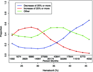
Figure 1: Proportion of person-months with 25% or greater increase or decrease in epoetin dose by current hematocrit (%) level.

1.3 Dynamic treatment regimens

We consider epoetin dosing strategies to be a type of dynamic treatment regimen. A deterministic dynamic treatment regimen is any sequential decision strategy, guideline or rule that defines how a subject’s current treatment depends on their measured covariate and possibly treatment histories. In the case of epoetin dosing, a treatment regimen constitutes the target hemoglobin or hematocrit range along with rules that dictate how the dose of epoetin should be adjusted over time. The specification of candidate treatment guidelines to be studied is a critical first step in the analysis process. Once the set of possible guidelines have been defined, one can retrospectively determine whether or not each subject’s treatment was compliant with a particular regimen, and then base analyses on those months that were adherent to the regimen under study. Since we wish to characterize survival under full compliance to a specific dosing guideline, subjects are typically censored at the first visit when their treatment trajectory no longer adheres to the regimen under study.

Currently, there are a limited number of statistical methods that permit direct estimation of the marginal (structural) performance of longitudinal treatment guidelines, and the evaluation of existing methods is quite limited with few worked examples and minimal simulation evaluation. An extensive review of relevant available methods is found in Chapter 5 of Chakraborty and Moodie (2013). Briefly, under appropriate assumptions, Inverse Probability of Censoring Weights (IPCW) and Marginal Structural Models (MSM) introduced in Robins (1993), Robins, Rotnitzky and Zhao (1995) and Robins, Hernán and Brumback (2000) can be used to adjust for measured time-dependent confounding and selection bias in observational studies. These methods were used in Hernán et al. (2006) to compare survival under two dynamic treatment regimens for the initiation of highly active antiretroviral therapy (HAART) in HIV-infected patients. Further analyses have compared multiple candidate CD4 cell count thresholds for the initiation of treatment. For example, Orellana, Rotnitzky and Robins (2010), Cain et al. (2010, 2011) have introduced methods for comparing multiple regimens by creating an artificial data set in which each subject contributes observations for each regimen they followed. Recently, Cotton and Heagerty (2011) consider dynamic guidelines and a data augmentation estimation method, and Shortreed and Moodie (2012) consider quantitative outcomes relying on the bootstrap for inference. Robins, Orellana and Rotnitzky (2008) also considered a $g$-estimation approach to finding the optimal regimen, while Young et al. (2011) focused on analyses using the parametric $g$-formula.

In this paper we focus on the evaluation of treatment guidelines that target achieving control of a particular intermediate covariate. The remainder of the article is structured as follows: in Section 2 we introduce notation and adapt the MSM methods of Cotton and Heagerty (2011) and Orellana, Rotnitzky and Robins (2010) to provide a general methodology for the comparison of treatment guidelines indexed by a finite parameter, and that map the observed dose history and intermediate marker history into a current dose assignment. In addition, we introduce a new simple weighted log-rank method to test for differences in the population survival distribution that would be realized under alternative dynamic regimens. This test extends ideas in Pepe and Couper (1997), Pepe, Heagerty and Whitaker (1999) and Zheng and Heagerty (2005). In Section 3 we present a simulation study using a new data generation structure that permits evaluation of statistical methods for evaluation of dynamic guidelines where the structural model can be directly determined to satisfy MSM assumptions. We also evaluate the use of clustered data sandwich standard errors which are known to be valid but potentially conservative when used with a MSM with estimated weights. In Section 4 we apply the methods to the USRDS data set of incident hemodialysis subjects. Our case study extends our previous work [Cotton and Heagerty (2011)] and illustrates the methods using a relatively long series of longitudinal data that drives adaptive treatments. As discussed in Section 1.1, there is clear medical motivation to study alternative guidelines in this setting. Finally, we conclude with a discussion in Section 5.

2 Methodology

2.1 Notation

Let $\mathbf{L}_{i}(t)$ be a vector of possibly time-varying covariates collected on the $i$th subject, $i=1,\ldots,n$, at the $t$th regularly spaced observation time, $t=0,1,2,\ldots.$ Denote the baseline covariates by $\mathbf{V}_{i}=\mathbf{L}_{i}(0)$. Let $Z_{i}(t)$ be the treatment (e.g., a drug dosage) prescribed at visit $t$. It is assumed that $Z_{i}(t)$ is determined following the collection of $\mathbf{L}_{i}(t)$ and may therefore be influenced by these covariates. Overbars are used to represent history up to and including time $t$ so that $\bar{\mathbf{L}}_{i}(t)=\{\mathbf{L}_{i}(s)\dvtx s=0,\ldots,t\}$. Finally, let $T_{i}$ be the event time of interest. Because we are dealing with data observed at discrete time points, the exact $T_{i}$ may not be available, so instead let $D_{i}(t)$ be the indicator of the event occurring in the time period $(t,t+1]$. Assume there is no loss to follow-up and the event is observed in all subjects. Later, this assumption can be relaxed by using weighting methods similar to those discussed in Section 2.3.

2.2 Parameterizing the treatment regimen

We will consider regimens that specify a range of acceptable treatment values for $Z_{i}(t)$ given a subject’s previous treatment value $Z_{i}(t-1)$ and a single time-varying covariate $L_{i}(t)_{1}$ [the first element of the vector $L_{i}(t)$]. For example, the regimen

$$Z_{i}(t)|Z_{i}(t-1),L_{i}(t)_{1},t>0\in\cases{Z_{i}(t-1)\times(p_{1},p_{2}),\cr\qquad\mbox{if $L_{i}(t)_{1}>b_{2}$,}\vspace*{3pt}\cr Z_{i}(t-1)\times(p_{3},p_{4}),\cr\qquad\mbox{if $L_{i}(t)_{1}\in[b_{1},b_{2}]$},\vspace*{3pt}\cr Z_{i}(t-1)\times(p_{5},p_{6}),\cr\qquad\mbox{if $L_{i}(t)_{1}<b_{1}$}}$$ (1)

specifies the range of allowable multiplicative changes $Z_{i}(t)$ based on whether $L_{i}(t)_{1}$ is above, within or below a target range of $(b_{1},b_{2})$. This type of regimen is quite flexible and is fully defined by the set of parameters ($p_{1}$, $p_{2}$, $p_{3}$, $p_{4}$, $p_{5}$, $p_{6}$, $b_{1}$, $b_{2}$). The regimen specification is easily generalizable to additive changes in dose or dependence on multiple time-varying covariates from $\bar{\mathbf{L}}_{i}(t)$.

2.3 Estimation: Creation of clones

For the methods that follow assume that it is unknown which, if any, of some $K$ treatment regimens of interest a subject was treated under. Depending on the regimen specifications, it may be possible for a subject to be adherent to multiple regimens at the same time. In order to accommodate this, we propose to clone (or replicate) each subject to create $K$ identical copies of their complete treatment and covariate history. Let $\mathbf{L}_{ik}(t)=\mathbf{L}_{i}(t)$ be the copied vector of time-varying covariates, $\mathbf{V}_{ik}=\mathbf{V}_{i}$ be the baseline covariates, $Z_{ik}(t)=Z_{i}(t)$ be the treatment dose and let $D_{ik}(t)=D_{i}(t)$ be the event indicator for subject $i$ under regimen $k$. Put another way, this refers to subject $i$’s $k$th clone where $k=1,\ldots,K$.

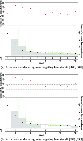
Figure 2: Illustration of cloning methodology with hematocrit and epoetin histories for one subject from the USRDS data set. Upper panels show monthly hematocrit (%) and lower panels show total monthly epoetin dose (10,000 units). In the lower panel the shaded grey regions indicate where the epoetin dose would have to fall in order to be compliant with a treatment regimen in the form of equation (1) with $(p_{1},p_{2},p_{3},p_{4},p_{5},p_{6})=(0,0.75,0.75,1.25,1.25,\infty)$.

Next, we retrospectively determine whether each subject was compliant with each treatment regimen. We use the terms compliance and adherence interchangeably and let $A_{ik}(t)=1$ indicate subject $i$’s adherence to regimen $k$ at time $t$. Otherwise, $A_{ik}(t)=0$. Each clone is artificially censored when they are no longer adherent with their treatment regimen, and any subject with zero adherence time to a specific regimen will have fewer than $K$ clones contribute to the analysis. Let $C_{ik}(t)$ be an indicator of artificial censoring for subject $i$ under regimen $k$ at time $t$. Note that the censoring is fully determined through the adherence history $\bar{A}_{ik}(t)$ and given by $C_{ik}(t)=1-I[\bar{A}_{ik}(t)=\bar{1}]$, where $\bar{1}$ is a vector of ones the same length as $\bar{A}_{ik}(t)$. So $C_{ik}$ is a vector of zeros followed by ones starting at the first nonadherent visit. Note that the use of the subscript $k$ on $\mathbf{V}_{ik}$, $D_{ik}(t)$, $Z_{ik}(t)$ and $\mathbf{L}_{ik}(t)$ is redundant since the cloning process does not alter the event time or follow-up data, as it simply defines the artificial censoring time based on adherence.

The key idea is that the creation of clones with appropriate regimen-specific nonadherence censoring allows us to compare survival under alternative dosing strategies. Weights are essential to correct for selection bias or for any factors associated with nonadherence to each specific regimen. For example, if we only had one regimen of interest, then we would create only one parsing of the longitudinal data to reflect observed adherence to the regimen under study (e.g., not create multiple clones) but would still need to consider weighting for valid inference regarding survival under the specific regimen.

If $A_{ik}(t)=A_{il}(t)=1$, we say that subject $i$ was coadherent to regimens $k$ and $l$ at time $t$. The concepts of cloning and coadherence are illustrated in Figure 2 with follow-up data from one subject from the USRDS data set. Both panels display the same observed hematocrit and epoetin dose histories. The upper and lower panels consider regimens targeting hematocrit ranges of $[30\%,36\%]$ and $[33\%,39\%]$, respectively. Both regimens specify an allowable multiplicative change in epoetin of plus or minus 25% when hematocrit is within the target. For each month, the grey shaded region indicates the range of epoetin doses that would have led to compliance with the regimen at that month. From the upper panel we see that the subject is compliant up to and including month seven. The lower panel indicates compliance to the higher target regimen up to month 11. So for months three through seven this subject was coadherent to both regimens. The subject is artificially censored at months 8 (upper panel) and 12 (lower panel).

The artificial censoring has the potential to induce selection bias. For example, if subjects with less severe disease, and hence longer survival times, are less likely to be censored under a particular regimen, the analysis set will be overrepresented by subjects with less severe disease. In an unadjusted analysis the effectiveness of the regimen would be overestimated. We use stabilized inverse probability weights (IPW) [Robins et al. (1992)] to attempt to adjust for this potential selection bias:

$$sw_{ik}(t)=\prod_{s=0}^{t}\frac{P[C_{ik}(s)=0|\bar{C}_{ik}(s-1)=\bar{0},V_{i}=v_{i}]}{P[C_{ik}(s)=0|\bar{C}_{ik}(s-1)=\bar{0},\bar{L}_{i}(s)=\bar{l}_{i}(s)]}.$$

At each time point, each clone is weighted by the inverse of the probability that they remained adherent to their treatment regimen given their measured covariate history. So adherent clones account for themselves as well as other similar subjects who were nonadherent to the regimen and therefore artificially censored. The model in the numerator includes only baseline covariates and serves to reduce the variability (i.e., stabilize) of the weights. This occurs because the probabilities in the numerator and denominator tend to be correlated. Details of the estimation of these weights have been well covered in the literature [Robins, Hernán and Brumback (2000), Hernán, Brumback and Robins (2001)]. Using these weights creates a pseudo-population in which the probability of remaining adherent is independent of measured confounders. In order for these methods to be valid, we must assume that the baseline and longitudinal information is sufficiently predictive of nonadherence to satisfy the assumption of effective sequential randomization [Hernán, Brumback and Robins (2001)]. We discuss assumptions in detail in the next section.

The above cloning process induces a unique correlation structure on the created clusters of data. Within-clone correlation exists over time due to the estimation of weights. The weights within clone sets are expected to be more similar over time than the weights between any two of a subject’s clones. However, between clone correlation also exists because, if observed (i.e., each clone remained uncensored under their respective regimen), both clones will have the same time of death.

We have induced a form of censoring and explicitly consider weights to adjust for this selection bias. However, additional selection bias or confounding may exist in an observational data set, and additional work may be needed to conduct valid inference. Additional weights can also be included to account for censoring due to loss to follow-up or administrative censoring.

2.3.1 Causal assumptions

Suppressing the subject subscript $i$, we assume for each possible history $\bar{a}$ there is a corresponding counterfactual event time $T_{\bar{a}}$. In the methods that follow we make the following assumptions. First, the sequential randomization or no unmeasured confounders assumption states that conditional on the observed covariate and treatment history, the treatment a subject received at time $t$ is independent of their counterfactual outcomes $T_{\bar{a}}$:

$$T_{\bar{a}}\coprod A(k)|\bar{A}(k-1)=\bar{a}(k-1),\bar{L}(k)=\bar{l}(k),T>u(k),$$

for all histories $\bar{a}(k-1)$ and $\bar{l}(k)$ where $u(k)$ is the time of visit $k$ [Hernán, Brumback and Robins (2001), Robins (1998, 2000)]. Next, the positivity assumption states that all subjects have a nonzero probability of being adherent to any regimen:

$$0<P\bigl{[}A(k)=1|\bar{A}(k-1)=\bar{a}(k-1),\bar{L}(k)=\bar{l}(k),T>u(k)\bigr{]}<1$$

with probability 1. Finally, we make the stable unit treatment value assumption that one subject’s potential outcome is not influenced by the treatment allocated to other subjects [Rubin (1980)].

2.4 Cloned IPW weighted log-rank test

Suppose there are two regimens of interest ($k=1,2$) and each subject has been cloned as outlined above so that for each subject the survival of clone $k$ is considered under regimen $k$. Essentially, this is paired survival data and in order to use a log-rank test, adjustments must be made for the correlation between pairs/clones. However, the IPW also needs to be incorporated to adjust for the selection bias induced by the artificial censoring. The cloned IPW weighted log-rank test presented here is an extension of the unpaired test described by Xie and Liu (2005) and relies on methods from Jung (1999) for calculating the standard error of the rank test statistic for paired survival data. The hypothesis to be tested is that the cumulative hazard functions are the same under the two regimens:

$$H_{0}\dvtx\Lambda_{1}(t) = \Lambda_{2}(t)\qquad\mbox{for all }0\leq t\leq\tau\qquad\mbox{versus}$$

$$H_{1}\dvtx\Lambda_{1}(t) \neq \Lambda_{2}(t)\qquad\mbox{for some }0\leq t\leq\tau,$$

where $\tau$ is the largest time at which both sets of clones have at least one subject at risk and $\Lambda_{1}(t)$ and $\Lambda_{2}(t)$ are the true underlying cumulative hazard functions. For subjects $i=1,\ldots,n$ let $(T_{i1},T_{i2})$ be the i.i.d. paired (cloned) survival times and $(C_{i1},C_{i2})$, $i=1,\ldots,n$ be the i.i.d. cloned censoring times. Then $X_{ik}=\min(T_{ik},C_{ik})$ is the observed event time and $\Delta_{ik}=I(T_{ik}\leq C_{ik})$ is the event indicator for subject $i$ under regimen $k=1,2$. So the full set of observed data is given by $\{(X_{i1},X_{i2},\Delta_{i1},\Delta_{i2})$, $i=1,\ldots,n\}$. Note that our unique cloning correlation structure implies that if $\Delta_{i1}=\Delta_{i2}=1$, then $T_{i1}=T_{i2}$.

Using standard survival analysis notation, the event process is given by $N_{ik}(t)=\Delta_{ik}I(X_{ik}\leq t)$, and $N_{k}(t)=\sum_{i=1}^{n}N_{ik}(t)$ is the total number of deaths observed under regimen $k$ at or before time $t$. The standard at risk process is given by $Y_{ik}(t)=I(t\leq X_{ik})$, so $Y_{k}(t)=\sum_{i=1}^{n}Y_{ik}(t)$ is the total number of subjects at risk at time $t$ under regimen $k$.

For each regimen assume that the true time-varying subject-specificweights are $w_{ik}(t)$ and that consistent estimates $\widehat{sw}_{ik}(t)$ are available. Now define a weighted event process through its derivative as $dN_{k}^{w}(t)=\break\sum_{i=1}^{n}\,dN_{ik}^{w}(t)$, where

$$dN_{ik}^{w}(t)=w_{ik}(t)\,dN_{ik}(t)=\cases{w_{ik}(X_{ik}),&\quad if $t=X_{ik}$ and $\Delta_{ik}=1$,\cr 0,&\quad otherwise}$$

and a weighted at risk process as $Y_{k}^{w}(t)=\sum_{i=1}^{n}Y_{ik}^{w}(t)$ where $Y_{ik}^{w}(t)=w_{ik}(t)\*I(X_{ik}\leq t)$. Recall the Nelson estimator of the cumulative hazard and define a corresponding weighted version:

$$\hat{\Lambda}_{k}(t)=\int_{0}^{t}\frac{dN_{k}(s)}{Y_{k}(s)},\qquad\hat{\Lambda}_{k}^{w}(t)=\int_{0}^{t}\frac{dN_{k}^{w}(s)}{Y_{k}^{w}(s)}.$$

Jung (1999) provides the details of a log-rank test with correlated survival times. With the addition of time-varying subject-specific weights, a natural extension of the standard class of rank statistics is

$$W^{*}=\sqrt{n}\int_{0}^{\infty}H(t)\bigl{[}d\hat{\Lambda}_{1}^{w}(t)-d\hat{\Lambda}_{2}^{w}(t)\bigr{]}$$

with

$$H(t)=\frac{1}{n}\frac{Y_{1}^{w}(t)Y_{2}^{w}(t)}{Y_{1}^{w}(t)+Y_{2}^{w}(t)}.$$

The statistic $W^{*}$ is equivalent to the usual form of the log-rank test statistic as the sum over time of the difference in the observed number of deaths in one group and the expected number of deaths in that group under $H_{0}$. For discrete time points $t=1,\ldots,T$ let $d_{k}(t)=\sum_{i=1}^{n}\Delta_{ik}I(X_{ik}=t)$ be the number of deaths observed in group $k$ at time $t$ and $d_{k}^{w}(t)=\sum_{i=1}^{n}w_{ik}(t)\Delta_{ik}I(X_{ik}=t)$ be the weighted number of deaths in group $k$ at time $t$. Then it can be shown that

$$W^{*}=\frac{1}{\sqrt{n}}\sum_{t=1}^{T}\biggl{[}d_{1}^{w}(t)-Y_{1}^{w}(t)\biggl{(}\frac{d_{1}^{w}(t)+d_{2}^{w}(t)}{Y_{1}^{w}(t)+Y_{2}^{w}(t)}\biggr{)}\biggr{]}.$$

In Appendix A in the supplementary material [Cotton and Heagerty (2014)] we derive the above form of $W^{*}$, show that under $H_{0}$, $W^{*}$ is asymptotically normal with mean 0 and variance $\sigma^{2}$, and give a consistent estimator for $\sigma^{2}$.

2.5 Cloned marginal structural Cox proportional hazards models

2.5.1 Comparison of two treatment regimens

The usual Cox proportional hazards adherence-based MSM [Hernán, Brumback and Robins (2000, 2001), Robins and Finkelstein (2000)] can be used with the cloned survival data provided that valid standard errors are used to account for the “clone clusters.” In the simplest setting of comparing two treatment regimens with known regimen membership at baseline, we can specify a proportional hazards marginal association model:

$$\lambda_{T}(t|G_{i},\mathbf{V}_{i})=\lambda_{0}(t)\exp\bigl{(}\beta_{1}G_{i}+\bolds\alpha^{\prime}\mathbf{V}_{i}\bigr{)},$$

where $\lambda_{0}(t)$ is an unspecified baseline hazard function, $G_{i}$ is an indicator of regimen assignment and $V_{i}$ is a set of baseline (nontime-varying) covariates. If there were no censoring/nonadherence and regimen membership $G_{i}$ had been randomly assigned, then there would be no confounding and the parameter $\beta_{1}$ would have a causal interpretation.

Specifically, $\exp(\beta_{1})$ is the causal hazard ratio comparing the two regimens. Most standard statistical software packages do not allow for the inclusion of subject-specific time-varying weights in fitting a Cox model. However, the model can be fit using weighted pooled logistic regression weighted by $\widehat{sw}_{i}(t)$ with each subject visit treated as a single observation:

$$\operatorname{logit}P\bigl{[}D_{i}(t)=1|D_{i}(t-1)=0,G_{i},\mathbf{V}_{i}\bigr{]}=\beta_{0}(t)+\beta_{1}G_{i}+\bolds\alpha^{\prime}\mathbf{V}_{i}.$$

Here $\beta_{0}(t)$ is a time-specific intercept usually fit as a spline. While this yields a consistent estimate of $\exp(\beta_{1})$, the estimated standard error may be invalid since the estimation of the weights induces a within-subject correlation. In order to overcome this, the model is fit using a Generalized Estimating Equations (GEE) approach with working independence [Liang and Zeger (1986)].

For the cloned data setting we proceed in the same manner but treat each of the $2n$ clones as independent observations. Let $G_{ik}=I[k=2]$ be the indicator that the clone is followed under regimen 2. To fit the MSM, each clone visit is now treated as a single observation in the logistic model:

$$\operatorname{logit}P\bigl{[}D_{ik}(t)=1|D_{ik}(t-1)=0,G_{ik},\mathbf{V}_{ik}\bigr{]}=\beta_{0}(t)+\beta_{1}G_{ik}+\bolds\alpha^{\prime}\mathbf{V}_{i}.$$

We assume working independence, but based on results in Lee, Wei and Amato (1992) for the Cox model, the estimated regression parameters will still be consistent. A consistent variance estimate can be obtained from the standard GEE sandwich covariance estimate if weights are known, and will provide conservative standard errors with estimated weights [Hernán, Brumback and Robins (2001)].

2.5.2 Extension to multiple treatment regimens

Instead of comparing just two treatment regimens, suppose there are multiple regimens to be compared simultaneously. Let $G_{ik}=k$, $k=1,2,\ldots,K$ indicate a clone’s treatment regimen assignment. There are a variety of different Cox proportional hazard MSMs that can be considered. In general, let

$$\lambda_{T}(t|G_{ik},\mathbf{V}_{i})=\lambda_{0}(t)\exp\bigl{[}\beta(G_{ik},t)+\bolds\alpha^{\prime}\mathbf{V}_{i}\bigr{]},$$ (2)

where $\beta(G_{ik},t)$ is a smooth function of both the observation time $t$ and the regimen number $G_{ik}$. Special cases of the above model include assuming a linear regimen effect $\beta(G_{ik},t)=\beta G_{ik}$ or treating regimen as a factor variable with or without interactions with time. A more flexible model would include splines in regimen number and/or the effect of time. The interpretation of $\beta$ will be as a causal hazard ratio, although the precise interpretation will depend on the model specification. We assume that the effect of the covariates $\mathbf{V}$ is constant across the comparison of any two regimens at any times.

3 Simulation study

A simulation study was undertaken to: (1) illustrate the structural models described above in a setting where counterfactual outcomes satisfy known relationships, (2) evaluate the performance of the point estimation strategy, and (3) evaluate the performance of the sandwich standard errors. The first and third of these goals have not been fully addressed in the existing literature.

For each of $K=6$ regimens we simulated $n_{k}=2500$ survival times using an exponential distribution with rate parameter $\lambda_{k}$. This generated continuous simulated survival times $T_{i}$ for $i=1,\ldots,n=\sum n_{k}={}$15,000 subjects each under full adherence to one regimen. We discretize $T_{i}$ to $D_{i}(t)=I[t<T_{i}\leq t+1]$, the indicator of death in the next time period. Let $\tilde{k}$ represent the regimen under which subject $i$’s survival time was generated. The adherence indicators for regimen $\tilde{k}$ are $A_{i\tilde{k}}(t)=1$ for $t=0,\ldots,\operatorname{int}(T_{i})$, where $\operatorname{int}(T_{i})$ is the largest integer less than $T_{i}$.

Each simulated subject is cloned and their adherence to the $K-1$ other regimens is simulated based on a set of fixed coadherence probabilities.The rate parameters $\lambda_{k}$ are selected in such a way that the hazard ratios $\lambda_{k}/\lambda_{3}$ for $k=2,4,5$ are the same for the original raw data and the cloned data. Details are given in Appendix B.1 in the supplementary material [Cotton and Heagerty (2014)]. The data generation method does not guarantee that the hazard ratios $\lambda_{1}/\lambda_{3}$ and $\lambda_{6}/\lambda_{3}$ are the same before and after the cloning, so the results for these two regimens are not included. To induce selection bias through artificial censoring, a scalar baseline covariate $V_{i}$ associated with both survival time and coadherence (and therefore censoring) is included. We consider three levels of selection bias: none, moderate and severe. For details, see Appendix B.2.

The concept of coadherence in the simulation study relates directly to the comparison of multiple treatment regimens. Consider two regimens of the form of equation (1) with overlapping target ranges. At any given month a subject is much more likely to be adherent to both these regimens than they would be to be adherent to two regimens with nonoverlapping target ranges. In addition, any baseline covariate that’s used in the decision of how to change treatment in response to changing hematocrit may be associated with coadherence of two regimens.

The aggregated results of 500 simulations are presented in Table 2. Regimen $k=3$ is considered the reference regimen. The first two columns of the table present the true underlying hazard ratios $\lambda_{k}/\lambda_{3}$ for $k=2,4,5$ and the median of the 500 estimated hazard ratios based on the original $n$ simulated fully compliant event times. The agreement between these two columns demonstrates that the true underlying hazard ratios can be estimated from the data despite the discretization of the event times.

Table 2: Estimated median hazard ratios (HR), empirical standard errors (ESE), average standard errors (ASE) and empirical 95% confidence interval coverages (ECP) from cloning methodology simulations at three levels of induced selection bias (500 replications each with $n_{k}=2500$)

	True HR	Complete data HR	Clones, unweighted				Clones, IPW weighted
Regimen			HR	ESE	ASE	ECP	HR	ESE	ASE	ECP
No induced selection bias
2 vs 3	0.91	0.90	0.89	0.0204	0.0233	92.8	0.89	0.0221	0.0232	90.6
4 vs 3	1.17	1.17	1.18	0.0305	0.0316	94.8	1.18	0.0330	0.0315	92.8
5 vs 3	1.28	1.29	1.31	0.0341	0.0352	90.2	1.31	0.0352	0.0357	88.2
Moderate selection bias
2 vs 3	0.91	0.90	0.89	0.0206	0.0230	94.2	0.89	0.0213	0.0225	92.4
4 vs 3	1.17	1.18	1.27	0.0308	0.0340	11.8	1.17	0.0301	0.0314	94.8
5 vs 3	1.28	1.29	1.40	0.0357	0.0376	09.2	1.30	0.0346	0.0355	92.8
Severe selection bias
2 vs 3	0.91	0.91	0.90	0.0217	0.0227	94.0	0.89	0.0217	0.0218	92.6
4 vs 3	1.17	1.18	1.37	0.0335	0.0365	00.0	1.17	0.0302	0.0314	96.4
5 vs 3	1.28	1.29	1.49	0.0416	0.0401	00.0	1.30	0.0362	0.0354	90.2

The next four columns present results from the cloned, unweighted data and demonstrate the effect of the selection bias induced through the coadherence probabilities described in Appendix B.2. In all scenarios the data was generated without selective nonadherence between regimens 2 and 3 and the median estimated hazard ratio and the coverage of the 95% confidence intervals just below the nominal level. The coadherence probabilities do induce substantial selection bias between regimens 4 and 3 and regimens 5 and 3. In the severe selection bias scenario the empirical coverage probability of the confidence intervals is zero.

The final four columns of Table 2 give the results of weighting the clones by the estimated IPW. A logistic model for adherence given the $V_{i}$ covariate is used for the weights. In all three scenarios the median estimated hazard ratios are very close to the truth. In the moderate and severe selection bias scenarios the coverage of the confidence intervals is greatly improved, although it is slightly below the nominal level in several cases. In cases without selection bias, we suspect that the lower than nominal coverage rates in the IPW analysis are due to instability of inefficiency of the IPW estimates after the inclusion of unnecessary weights. The empirical and average standard errors for the unweighted and weighted clones are comparable. This supports the claim that the zero coverage in the unweighted case is due to bias in the estimates as opposed to underestimating the variance.

4 Application to USRDS data set

In this section we apply the cloning methodology to a large data set from the USRDS introduced in Section 1.2. Analysis begins at month 3 (since the initial dosing strategy is different from the maintenance dosing strategy that we wish to study), with up to 9 months of follow-up data per subject ($t=0,\ldots,9$).

4.1 Naive analyses

First we use Cox proportional hazards regression to conduct naive analyses of the acute association between mortality and epoetin dose. The last month’s assigned dose is treated as a time-dependent covariate in models adjusted for baseline covariates (age, sex, race, diabetes and hypertension). Models are fit both with and without time-dependent hematocrit (measured as the average of the last two months’ values). Both models yield essentially the same result. The estimated log hazard ratio associated with one unit increase in epoetin dose is 0.031 (0.028, 0.034), suggesting that higher epoetin doses are associated with an increased risk of mortality, as one would expect higher hematocrit levels are associated with a reduced risk of mortality [log hazard ratio of $-$0.035 ($-$0.032, $-$0.038)]. The naive analysis is difficult to translate into recommendations for epoetin dosing strategies since trying to attain a high hematocrit level and a low epoetin dose may be incompatible in most patients.

4.2 Dynamic treatment regimens for epoetin dosing

We consider multiple dynamic treatment regimens for epoetin dose $Z_{i}(t)$ given current hematocrit level $L_{i}(t)_{1}$ and previous dose $Z_{i}(t-1)$ of the form in equation (1), where

$$Z_{i}(t)|Z_{i}(t-1),L_{i}(t)_{1},t>0\in\cases{Z_{i}(t-1)\times\bigl{(}-\infty,-(1-p)\bigr{)},\cr\qquad\mbox{if $L_{i}(t)_{1}>x-3$},\vspace*{3pt}\cr Z_{i}(t-1)\times(0.75,1.25),\cr\qquad\mbox{if $L_{i}(t)_{1}\in[x-3,x+3]$,}\vspace*{3pt}\cr Z_{i}(t-1)\times\bigl{(}(1+p),\infty\bigr{)},\cr\qquad\mbox{if $L_{i}(t)_{1}<x+3$,}}$$

with $x$ representing the midpoint of the target hematocrit range of $(x-3,x+3)$ and $p$ controlling the allowable multiplicative change in dose outside the target range. We consider regiments with $x=31,\ldots,40$ and $p=0.05,\ldots,0.50$ in $0.05$ increments and refer to the regimens by the notation $\mathcal{G}(p,x-3,x+3)$. The regimen $\mathcal{G}(0.25,30,36)$ is used as the baseline regimen for comparison purposes. A target range of $[30\%,36\%]$ was selected to mimic the subnormal targets used in several of the clinical trials referenced in Section 1.1.

The logistic model for the denominator of the IPW includes a spline in time along with the baseline covariates gender, age, race and indicators of diabetes and hypertension and the time-varying covariates previous month’s total epoetin dose and indicators of whether the average of the current and previous hematocrit was in the ranges $(0,28]$, $(28,32]$, $(36,40]$, $(40,\infty)$, as well as the difference between the current and the previous hematocrit. The model for the numerator was the same as above but did not include the time-varying covariates. Additional weights were calculated for administrative censoring (i.e., clones who were still alive and compliant to their regimen at month 12) and censoring due to loss to follow-up (i.e., clones who were alive and compliant at a final recorded visit occurred prior to month 12). All weight models were stratified by regimen. The three stabilized weights were multiplied to give the final weight used in the analyses. The weight specification is key for valid causal inference. All available potential confounders, in particular, key variables known to drive changes in epoetin dosing and epoetin response [for a summary see Table 1 of Miskulin et al. (2009)], were included in the model to guard as best as possible against potential violation of the no unmeasured confounders assumption. However, we did not have access to detailed lab data nor do we have clinic data for additional adjustment and we acknowledge these potential limitations.

4.3 Results of cloned IPW weighted log-rank test

The cloned IPWweighted log-rank test from Section 2.4 was applied testing the equivalence of survival under various regimens with $\mathcal{G}(0.25,30,36)$. The results of a subset of the tests are given in Table 3. We reject the null hypothesis that the two survivor functions are equal ($p<0.05$) in all cases except the comparisons of $\mathcal{G}(0.10,30,36)$ and $\mathcal{G}(0.40,30,36)$ [the two regimens that share a common hematocrit target range with the reference regimen $\mathcal{G}(0.25,30,36)$] and $\mathcal{G}(0.40,32,38)$ (a regimen with a slightly higher target range and requiring more aggressive epoetin dose changes). The results of these tests indicate that there are significant differences in survival across possible epoetin dosing regimens. We will proceed with a regression analysis to try and capture trends in the survival across regimens.

=250pt $\bolds{p}$ 0.10 0.25 0.40 31 $<$0.032 $<$0.001 $<$0.001 33 $<$0.114 Reference $<$0.423 $x$ 35 $<$0.001 $<$0.006 $<$0.077 37 $<$0.001 $<$0.001 $<$0.001 39 $<$0.001 $<$0.001 $<$0.001

Table 3: Results of cloned IPW weighted log-rank test, USRDS data, $p$-values for tests of regimens $\mathcal{G}(p,x-3,x+3)$ versus regimen $\mathcal{G}(0.25,30,36)$

4.4 Cloned MSM results

Several models of the form of equation (2) have been fit to the data. The comparison of target hematocrit ranges is of primary interest, so the focus in on comparison of the regimens $\mathcal{G}(0.25,x-3,x+3)$. In models where regimen number is considered as a linear variable, the regimens are ordered by increasing target range midpoint. In models where regimen number is treated as a factor variable, pairwise comparisons between the regimen $\mathcal{G}(0.25,30,36)$ and the nine other regimens with $p=0.25$ are considered. [2.]

The estimated causal log hazard ratio for a one unit increase in regimen number is $-$0.017 ($-$0.022, $-$0.011). This is equivalent to a causal hazard ratio of 0.983 (0.978, 0.989), suggesting that regimens that target higher hematocrit ranges provide a small but statistically significant reduction in mortality.

The estimated causal hazard ratios comparing each treatment regimen with $\mathcal{G}(0.25,30,36)$ are presented in Table 4. These results also suggest that regimens targeting a higher hematocrit range yield a higher rate of survival. The hazard ratios are significantly different from one another for regimens targeting a range of $[34\%,40\%]$ or higher.

Table 5 gives the fitted causal hazard ratios for a one unit increase in regimen number at each observation month. For all months after month 3 (the baseline month) the hazard ratio is statistically significantly less than zero, suggesting that survival improves as the hematocrit target range midpoint increases. There is a trend in decreasing hazard ratio over time, suggesting that at later months there is an increased effect of treating with a regimen targeting a higher range.

=250pt Regimen comparison Hazard ratio 95% CI $\mathcal{G}(0.25,28,34)$ vs $\mathcal{G}(0.25,30,36)$ 1.056 (0.985, 1.132) $\mathcal{G}(0.25,29,35)$ vs $\mathcal{G}(0.25,30,36)$ 1.027 (0.959, 1.101) $\mathcal{G}(0.25,30,36)$ vs $\mathcal{G}(0.25,30,36)$ Reference – $\mathcal{G}(0.25,31,37)$ vs $\mathcal{G}(0.25,30,36)$ 0.984 (0.919, 1.054) $\mathcal{G}(0.25,32,38)$ vs $\mathcal{G}(0.25,30,36)$ 0.958 (0.895, 1.026) $\mathcal{G}(0.25,33,39)$ vs $\mathcal{G}(0.25,30,36)$ 0.940 (0.878, 1.006) $\mathcal{G}(0.25,34,40)$ vs $\mathcal{G}(0.25,30,36)$ 0.920 (0.859, 0.985) $\mathcal{G}(0.25,35,41)$ vs $\mathcal{G}(0.25,30,36)$ 0.913 (0.853, 0.977) $\mathcal{G}(0.25,36,42)$ vs $\mathcal{G}(0.25,30,36)$ 0.915 (0.854, 0.980) $\mathcal{G}(0.25,37,43)$ vs $\mathcal{G}(0.25,30,36)$ 0.915 (0.855, 0.980)

Table 4: Estimated hazard ratios from a cloned Cox marginal structural model (MSM), regimen treated as a factor variable with reference $\mathcal{G}(0.25,30,36)$, USRDS data

=250pt Month Hazard ratio 95% CI 3 0.999 (0.993, 1.004) 4 0.950 (0.940, 0.959) 5 0.914 (0.898, 0.930) 6 0.885 (0.864, 0.907) 7 0.862 (0.837, 0.887) 8 0.842 (0.814, 0.871) 9 0.825 (0.794, 0.857) 10 0.810 (0.777, 0.845) 11 0.797 (0.761, 0.834) 12 0.785 (0.747, 0.824)

Table 5: Estimated hazard ratios by month for a one unit increase in the midpoint of the target hematocrit range $x$ in regimens $\mathcal{G}(0.25,x-3,x+3)$, cloned Cox marginal structural model (MSM), linear regimen effect with a log time interaction, USRDS data

Recall that in this model within each regimen pair the log hazard ratio is assumed to be linear in $\log t$. A plot of the estimated causal log hazard ratios and pointwise 95% confidence intervals at month 9 is given in Figure 3. Informally, in both graphs an initial downward trend in estimates is seen for regimens with higher target ranges followed by possibly a flatter trend at the highest target ranges. The causal log hazard ratio for full compliance to the regimen $\mathcal{G}(0.25,34,40)$ to survival under full compliance to the regimen $\mathcal{G}(0.25,30,36)$ was $-$0.51 $(-0.77,-0.25)$ at month 6 and $-$0.80 $(-1.22,-0.37)$ at month 9.

These four models all show the same trend in survival when considering the regimens $\mathcal{G}(0.25,x-3,x+3)$, $x=31,\ldots,40$ as defined above. In general, regimens with target ranges above the reference range of $[30\%,36\%]$ provide a survival advantage when compared to $\mathcal{G}(0.25,30,36)$. These gains persisted with the inclusion of log(month) in the model. It is apparent in Figure 3 that while regimens with a higher target range yield a survival advantage, the improvement remains relatively constant for regimens with targets at or above $[34\%,40\%]$.

Similar models to those above were fit to the data for regimens, allowing varying multiplicative changes in epoetin doses outside the target range. The specific results are not reported here, but in general there were small (statistically insignificant) survival advantages for regimens with smaller $p$, that is, those that allowed smaller changes in epoetin dose when hematocrit was outside the $[30\%,36\%]$ target range.

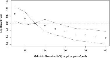
Figure 3: Estimated log hazard ratios at 9 months for regimens $\mathcal{G}(0.25,x-3,x+3)$ versus regimen $\mathcal{G}(0.25,30,36)$, cloned Cox marginal structural model (MSM), regimen treated as a factor variable with a log time interaction, USRDS data.

5 Discussion

In this article we detailed a cloning methodology for comparing dynamic treatment regimens when regimen membership is not known at baseline. Our goal was to perform an appropriate analysis of motivating data from dialysis patients. In order to implement cloning methods, we first detailed a simple log-rank test, and then proposed use of clustered survival methods for regression inference. In order to evaluate the proposed methods, we provide a novel simulation scenario that can control the structural parameters. The methods are based on replicating or cloning each subject and considering the adherence of each clone’s treatment history to a particular treatment regimen under consideration. Clones are artificially censored at their first nonadherent observation and IPW are used to adjust for the induced selection bias. If there are only two treatment regimens under comparison, we have shown that a cloned IPW weighted log-rank test can be used to test for equality of the survivor functions. The proposed variance estimator appropriately adjusts for the correlation within clones. When multiple treatment regimens are under consideration a Cox proportional hazards adherence-based MSM can be used to compare survival under the regimens. The structural regression model can take a variety of forms. In particular, one can choose to model regimen number as a linear or factor variable and choose whether or not to include interactions with time. In all cases, a consistent estimate of the causal hazard ratio is available.

For epoetin dosing in incident ESRD hemodialysis subjects, we have applied this methodology to a large USRDS data set to compare survival across multiple treatment regimens. As a demonstration, a variety of models were fit, but all essentially gave the same conclusion. Subjects tend to experience lower all-cause mortality when treated under epoetin dosing rules with higher hematocrit target ranges. However, there is evidence that there is no further gain in survival under regimens with targets above $[34\%,40\%]$. This result is scientifically meaningful, especially in light of the uncertainty in best practice for the treatment of CKD/ESRD-associated anemia.

This methodology is appealing because there is no requirement that regimens under consideration be of the same form. In fact, as long as adherence can be precisely determined, the treatment regimens can be extremely complex and depend on multiple time-varying covariates or prognostic factors. Through cloning, all subjects contribute information to all regimens to which they were continuously adherent. However, due to artificial censoring, any follow-up after a nonadherent visit is discarded. Further work is warranted to explore methods that might overcome or relax this requirement.

The current methods do not explicitly distinguish between different types of adherence (above, within or below target). A possible extension would be to include patient status relative to the target in the adherence model. Alternatively, it would be possible to consider adherence as a multinomial variable and simultaneously model the different types of nonadherence, for example, nonadherence due to insufficient increase in dose when the subject is below target, insufficient dose decrease when above target, unnecessary dose increase when within target or unnecessary dose decrease when within target. This would complicate the definition of the stabilized weights but warrants further investigation.

References

- Besarab et al. (1998) {barticle}[author] \bauthor\bsnmBesarab, \bfnmAnatole\binitsA., \bauthor\bsnmBolton, \bfnmW. Kline\binitsW. K., \bauthor\bsnmBrowne, \bfnmJeffrey K.\binitsJ. K., \bauthor\bsnmEgrie, \bfnmJoan C.\binitsJ. C., \bauthor\bsnmNissenson, \bfnmAllen R.\binitsA. R., \bauthor\bsnmOkamoto, \bfnmDouglas M.\binitsD. M., \bauthor\bsnmSchwab, \bfnmSteve J.\binitsS. J. and \bauthor\bsnmGoodkin, \bfnmDavid A.\binitsD. A. (\byear1998). \btitleThe effects of normal as compared with low hematocrit values in patients with cardiac disease who are receiving hemodialysis and epoetin. \bjournalN. Engl. J. Med. \bvolume339 \bpages584–590. \bnotePMID: 9718377. \bptokimsref\endbibitem
- Brookhart et al. (2010) {barticle}[author] \bauthor\bsnmBrookhart, \bfnmM. Alan\binitsM. A., \bauthor\bsnmSchneeweiss, \bfnmSebastian\binitsS., \bauthor\bsnmAvorn, \bfnmJerry\binitsJ., \bauthor\bsnmBradbury, \bfnmBrian D.\binitsB. D., \bauthor\bsnmLiu, \bfnmJun\binitsJ. and \bauthor\bsnmWinkelmayer, \bfnmWolfgang C.\binitsW. C. (\byear2010). \btitleComparative mortality risk of anemia management practices in incident hemodialysis patients. \bjournalJAMA: The Journal of the American Medical Association \bvolume303 \bpages857–864. \bptokimsref\endbibitem
- Cain et al. (2010) {barticle}[mr] \bauthor\bsnmCain, \bfnmLauren E.\binitsL. E., \bauthor\bsnmRobins, \bfnmJames M.\binitsJ. M., \bauthor\bsnmLanoy, \bfnmEmilie\binitsE., \bauthor\bsnmLogan, \bfnmRoger\binitsR., \bauthor\bsnmCostagliola, \bfnmDominique\binitsD. and \bauthor\bsnmHernán, \bfnmMiguel A.\binitsM. A. (\byear2010). \btitleWhen to start treatment? A systematic approach to the comparison of dynamic regimes using observational data. \bjournalInt. J. Biostat. \bvolume6 \bpagesArt. 18, 26. \biddoi=10.2202/1557-4679.1212, issn=1557-4679, mr=2644387 \bptokimsref\endbibitem
- Cain et al. (2011) {barticle}[pbm] \bauthor\bsnmCain, \bfnmLauren E.\binitsL. E., \bauthor\bsnmLogan, \bfnmRoger\binitsR., \bauthor\bsnmRobins, \bfnmJames M.\binitsJ. M., \bauthor\bsnmSterne, \bfnmJonathan A. C.\binitsJ. A. C., \bauthor\bsnmSabin, \bfnmCaroline\binitsC., \bauthor\bsnmBansi, \bfnmLoveleen\binitsL., \bauthor\bsnmJustice, \bfnmAmy\binitsA., \bauthor\bsnmGoulet, \bfnmJoseph\binitsJ., \bauthor\bparticlevan \bsnmSighem, \bfnmArd\binitsA., \bauthor\bparticlede \bsnmWolf, \bfnmFrank\binitsF., \bauthor\bsnmBucher, \bfnmHeiner C.\binitsH. C., \bauthor\bparticlevon \bsnmWyl, \bfnmViktor\binitsV., \bauthor\bsnmEsteve, \bfnmAnna\binitsA., \bauthor\bsnmCasabona, \bfnmJordi\binitsJ., \bauthor\bparticledel \bsnmAmo, \bfnmJulia\binitsJ., \bauthor\bsnmMoreno, \bfnmSantiago\binitsS., \bauthor\bsnmSeng, \bfnmRemonie\binitsR., \bauthor\bsnmMeyer, \bfnmLaurence\binitsL., \bauthor\bsnmPerez-Hoyos, \bfnmSantiago\binitsS., \bauthor\bsnmMuga, \bfnmRoberto\binitsR., \bauthor\bsnmLodi, \bfnmSara\binitsS., \bauthor\bsnmLanoy, \bfnmEmilie\binitsE., \bauthor\bsnmCostagliola, \bfnmDominique\binitsD. and \bauthor\bsnmHernan, \bfnmMiguel A.\binitsM. A. (\byear2011). \btitleWhen to initiate combined antiretroviral therapy to reduce mortality and AIDS-defining illness in HIV-infected persons in developed countries: An observational study. \bjournalAnn. Intern. Med. \bvolume154 \bpages509–515. \biddoi=10.7326/0003-4819-154-8-201104190-00001, issn=1539-3704, mid=NIHMS411085, pii=154/8/509, pmcid=3610527, pmid=21502648 \bptokimsref\endbibitem
- Canadian Erythropoietin Study Group (1990) {barticle}[author] \bauthor\bsnmCanadian Erythropoietin Study Group (\byear1990). \btitleAssociation between recombinant human erythropoietin and quality of life and exercise capacity of patients receiving haemodialysis. \bjournalBMJ \bvolume300 \bpages573–578. \bptokimsref\endbibitem
- Chakraborty and Moodie (2013) {bbook}[mr] \bauthor\bsnmChakraborty, \bfnmBibhas\binitsB. and \bauthor\bsnmMoodie, \bfnmErica E. M.\binitsE. E. M. (\byear2013). \btitleStatistical Methods for Dynamic Treatment Regimes. \bpublisherSpringer, \blocationNew York. \biddoi=10.1007/978-1-4614-7428-9, mr=3112454 \bptokimsref\endbibitem
- Cotton and Heagerty (2011) {barticle}[author] \bauthor\bsnmCotton, \bfnmC. A.\binitsC. A. and \bauthor\bsnmHeagerty, \bfnmP. J.\binitsP. J. (\byear2011). \btitleA data augmentation method for estimating the causal effect of adherence to treatment regimens targeting control of an intermediate measure. \bjournalStatistics in Biosciences \bvolume3 \bpages28–44. \bptokimsref\endbibitem
- Cotton and Heagerty (2014) {bmisc}[author] \bauthor\bsnmCotton, \binitsC. A. and \bauthor\bsnmHeagerty, \binitsP. J. (\byear2014). \bhowpublishedSupplement to “Evaluating epoetin dosing strategies using observational longitudinal data.” DOI:\doiurl10.1214/14-AOAS774SUPP. \bptokimsref \endbibitem\bptokimsref\endbibitem
- Drüeke et al. (2006) {barticle}[auto] \bauthor\bsnmDrüeke, \bfnmTilman B.\binitsT. B., \bauthor\bsnmLocatelli, \bfnmFrancesco\binitsF., \bauthor\bsnmClyne, \bfnmNaomi\binitsN., \bauthor\bsnmEckardt, \bfnmKai-Uwe\binitsK.-U., \bauthor\bsnmMacdougall, \bfnmIain C.\binitsI. C., \bauthor\bsnmTsakiris, \bfnmDimitrios\binitsD., \bauthor\bsnmBurger, \bfnmHans-Ulrich\binitsH.-U. and \bauthor\bsnmScherhag, \bfnmArmin\binitsA. (\byear2006). \btitleNormalization of hemoglobin level in patients with chronic kidney disease and anemia. \bjournalN. Engl. J. Med. \bvolume355 \bpages2071–2084. \bptokimsref\endbibitem
- Eschbach (1994) {barticle}[author] \bauthor\bsnmEschbach, \bfnmJ. W.\binitsJ. W. (\byear1994). \btitleErythropoietin: The promise and the facts. \bjournalKidney International Supplements \bvolume44 \bpagesS70–S76. \bptokimsref\endbibitem
- Hernán, Brumback and Robins (2000) {barticle}[pbm] \bauthor\bsnmHernán, \bfnmM. A.\binitsM. A., \bauthor\bsnmBrumback, \bfnmB.\binitsB. and \bauthor\bsnmRobins, \bfnmJ. M.\binitsJ. M. (\byear2000). \btitleMarginal structural models to estimate the causal effect of zidovudine on the survival of HIV-positive men. \bjournalEpidemiology \bvolume11 \bpages561–570. \bidissn=1044-3983, pmid=10955409 \bptokimsref\endbibitem
- Hernán, Brumback and Robins (2001) {barticle}[mr] \bauthor\bsnmHernán, \bfnmMiguel A.\binitsM. A., \bauthor\bsnmBrumback, \bfnmBabette\binitsB. and \bauthor\bsnmRobins, \bfnmJames M.\binitsJ. M. (\byear2001). \btitleMarginal structural models to estimate the joint causal effect of nonrandomized treatments. \bjournalJ. Amer. Statist. Assoc. \bvolume96 \bpages440–448. \biddoi=10.1198/016214501753168154, issn=0162-1459, mr=1939347 \bptokimsref\endbibitem
- Hernán et al. (2006) {barticle}[author] \bauthor\bsnmHernán, \bfnmM. A.\binitsM. A., \bauthor\bsnmLanoy, \bfnmE.\binitsE., \bauthor\bsnmCostagliola, \bfnmD.\binitsD. and \bauthor\bsnmRobins, \bfnmJ. M.\binitsJ. M. (\byear2006). \btitleComparison of dynamic treatment regimes via inverse probability weighting. \bjournalBasic Clin. Pharmacol. Toxicol. \bvolume98 \bpages237–242. \bptokimsref\endbibitem
- Jung (1999) {barticle}[mr] \bauthor\bsnmJung, \bfnmSin-Ho\binitsS.-H. (\byear1999). \btitleRank tests for matched survival data. \bjournalLifetime Data Anal. \bvolume5 \bpages67–79. \biddoi=10.1023/A:1009635201363, issn=1380-7870, mr=1750342 \bptokimsref\endbibitem
- Lee, Wei and Amato (1992) {bincollection}[mr] \bauthor\bsnmLee, \bfnmEric W.\binitsE. W., \bauthor\bsnmWei, \bfnmL. J.\binitsL. J. and \bauthor\bsnmAmato, \bfnmDavid A.\binitsD. A. (\byear1992). \btitleCox-type regression analysis for large numbers of small groups of correlated failure time observations. In \bbooktitleSurvival Analysis: State of the Art (Columbus, OH, 1991) (\beditor\bfnmJ. P.\binitsJ. P. \bsnmKlein and \beditor\bfnmP. K\binitsP. K. \bsnmGoel, eds.) \bpages237–247. \bpublisherKluwer Academic, \blocationDordrecht. \bidmr=1175646 \bptnotecheck related \bptokimsref\endbibitem
- Liang and Zeger (1986) {barticle}[mr] \bauthor\bsnmLiang, \bfnmKung Yee\binitsK. Y. and \bauthor\bsnmZeger, \bfnmScott L.\binitsS. L. (\byear1986). \btitleLongitudinal data analysis using generalized linear models. \bjournalBiometrika \bvolume73 \bpages13–22. \biddoi=10.1093/biomet/73.1.13, issn=0006-3444, mr=0836430 \bptokimsref\endbibitem
- Miskulin et al. (2009) {barticle}[auto] \bauthor\bsnmMiskulin, \bfnmDana C.\binitsD. C., \bauthor\bsnmWeiner, \bfnmDaniel E.\binitsD. E., \bauthor\bsnmTighiouart, \bfnmHocine\binitsH., \bauthor\bsnmLadik, \bfnmVladimir\binitsV., \bauthor\bsnmServilla, \bfnmKaren\binitsK., \bauthor\bsnmZager, \bfnmPhilip G.\binitsP. G., \bauthor\bsnmMartin, \bfnmAlice\binitsA., \bauthor\bsnmJohnson, \bfnmH. K.\binitsH. K. and \bauthor\bsnmMeyer, \bfnmKlemens B.\binitsK. B. (\byear2009). \btitleComputerized decision support for EPO dosing in hemodialysis patients. \bjournalAm. J. Kidney Dis. \bvolume54 \bpages1081–1088. \bptokimsref\endbibitem
- Miskulin et al. (2013) {barticle}[author] \bauthor\bsnmMiskulin, \bfnmDana C.\binitsD. C., \bauthor\bsnmZhou, \bfnmJing\binitsJ., \bauthor\bsnmTangri, \bfnmNavdeep\binitsN., \bauthor\bsnmBandeen-Roche, \bfnmKaren\binitsK., \bauthor\bsnmCook, \bfnmCourtney\binitsC., \bauthor\bsnmEphraim, \bfnmPatti L.\binitsP. L., \bauthor\bsnmCrews, \bfnmDeidra C.\binitsD. C., \bauthor\bsnmScialla, \bfnmJulia J.\binitsJ. J., \bauthor\bsnmSozio, \bfnmStephen M.\binitsS. M., \bauthor\bsnmShafi, \bfnmTariq\binitsT. \betalet al. (\byear2013). \btitleTrends in anemia management in US hemodialysis patients 2004–2010. \bjournalBMC Nephrology \bvolume14 \bpages264. \bptokimsref\endbibitem
- National Kidney Foundation (2006) {barticle}[author] \bauthor\bsnmNational Kidney Foundation (\byear2006). \btitleK/DOQI clinical practice guidelines and clinical practice recommendations for anemia in chronic kidney disease. \bjournalAmerican Journal of Kidney Diseases \bvolume47: Suppl 3 \bpagesS11–S145. \bptokimsref\endbibitem
- Orellana, Rotnitzky and Robins (2010) {barticle}[mr] \bauthor\bsnmOrellana, \bfnmLiliana\binitsL., \bauthor\bsnmRotnitzky, \bfnmAndrea\binitsA. and \bauthor\bsnmRobins, \bfnmJames M.\binitsJ. M. (\byear2010). \btitleDynamic regime marginal structural mean models for estimation of optimal dynamic treatment regimes, Part I: Main content. \bjournalInt. J. Biostat. \bvolume6 \bpagesArt. 8, 49. \bidissn=1557-4679, mr=2602551 \bptokimsref\endbibitem
- Palmer et al. (2010) {barticle}[pbm] \bauthor\bsnmPalmer, \bfnmSuetonia C.\binitsS. C., \bauthor\bsnmNavaneethan, \bfnmSankar D.\binitsS. D., \bauthor\bsnmCraig, \bfnmJonathan C.\binitsJ. C., \bauthor\bsnmJohnson, \bfnmDavid W.\binitsD. W., \bauthor\bsnmTonelli, \bfnmMarcello\binitsM., \bauthor\bsnmGarg, \bfnmAmit X.\binitsA. X., \bauthor\bsnmPellegrini, \bfnmFabio\binitsF., \bauthor\bsnmRavani, \bfnmPietro\binitsP., \bauthor\bsnmJardine, \bfnmMeg\binitsM., \bauthor\bsnmPerkovic, \bfnmVlado\binitsV., \bauthor\bsnmGraziano, \bfnmGiusi\binitsG., \bauthor\bsnmMcGee, \bfnmRichard\binitsR., \bauthor\bsnmNicolucci, \bfnmAntonio\binitsA., \bauthor\bsnmTognoni, \bfnmGianni\binitsG. and \bauthor\bsnmStrippoli, \bfnmGiovanni F. M.\binitsG. F. M. (\byear2010). \btitleMeta-analysis: Erythropoiesis-stimulating agents in patients with chronic kidney disease. \bjournalAnn. Intern. Med. \bvolume153 \bpages23–33. \biddoi=10.7326/0003-4819-153-1-201007060-00252, issn=1539-3704, pii=0003-4819-153-1-201007060-00252, pmid=20439566 \bptokimsref\endbibitem
- Pepe and Couper (1997) {barticle}[mr] \bauthor\bsnmPepe, \bfnmMargaret Sullivan\binitsM. S. and \bauthor\bsnmCouper, \bfnmDavid\binitsD. (\byear1997). \btitleModeling partly conditional means with longitudinal data. \bjournalJ. Amer. Statist. Assoc. \bvolume92 \bpages991–998. \biddoi=10.2307/2965563, issn=0162-1459, mr=1482129 \bptokimsref\endbibitem
- Pepe, Heagerty and Whitaker (1999) {barticle}[author] \bauthor\bsnmPepe, \bfnmM. S.\binitsM. S., \bauthor\bsnmHeagerty, \bfnmP. J.\binitsP. J. and \bauthor\bsnmWhitaker, \bfnmR.\binitsR. (\byear1999). \btitlePrediction using partly conditional time-varying coefficients regression models. \bjournalBiometrics \bvolume55 \bpages944–950. \bptokimsref\endbibitem
- Pfeffer et al. (2009) {barticle}[auto] \bauthor\bsnmPfeffer, \bfnmMarc A.\binitsM. A., \bauthor\bsnmBurdmann, \bfnmEmmanuel A.\binitsE. A., \bauthor\bsnmChen, \bfnmChao-Yin\binitsC.-Y., \bauthor\bsnmCooper, \bfnmMark E.\binitsM. E., \bauthor\bparticlede \bsnmZeeuw, \bfnmDick\binitsD., \bauthor\bsnmEckardt, \bfnmKai-Uwe\binitsK.-U., \bauthor\bsnmFeyzi, \bfnmJan M.\binitsJ. M., \bauthor\bsnmIvanovich, \bfnmPeter\binitsP., \bauthor\bsnmKewalramani, \bfnmReshma\binitsR., \bauthor\bsnmLevey, \bfnmAndrew S.\binitsA. S., \bauthor\bsnmLewis, \bfnmEldrin F.\binitsE. F., \bauthor\bsnmMcGill, \bfnmJanet B.\binitsJ. B., \bauthor\bsnmMcMurray, \bfnmJohn J. V.\binitsJ. J. V., \bauthor\bsnmParfrey, \bfnmPatrick\binitsP., \bauthor\bsnmParving, \bfnmHans-Henrik\binitsH.-H., \bauthor\bsnmRemuzzi, \bfnmGiuseppe\binitsG., \bauthor\bsnmSingh, \bfnmAjay K.\binitsA. K., \bauthor\bsnmSolomon, \bfnmScott D.\binitsS. D. and \bauthor\bsnmToto, \bfnmRobert\binitsR. (\byear2009). \btitleA trial of darbepoetin alfa in type 2 diabetes and chronic kidney disease. \bjournalN. Engl. J. Med. \bvolume361 \bpages2019–2032. \bptokimsref\endbibitem
- Robins (1993) {binproceedings}[author] \bauthor\bsnmRobins, \bfnmJ. M.\binitsJ. M. (\byear1993). \btitleInformation recovery and bias adjustment in proportional hazards regression analysis of randomized trials using surrogate markers. In \bbooktitleProceedings of the Biopharmaceutical Section, American Statistical Association \bpages24–33. \bpublisherAmerican Statistical Association, \blocationAlexandria, VA. \bptokimsref\endbibitem
- Robins (1998) {binproceedings}[author] \bauthor\bsnmRobins, \bfnmJ. M.\binitsJ. M. (\byear1998). \btitleMarginal structural models. In \bbooktitle1997 Proceedings of the Section on Bayesian Statistical Science \bpages1–10. \bpublisherAmerican Statistical Association, \blocationAlexandria, VA. \bptokimsref\endbibitem
- Robins (2000) {bincollection}[mr] \bauthor\bsnmRobins, \bfnmJames M.\binitsJ. M. (\byear2000). \btitleMarginal structural models versus structural nested models as tools for causal inference. In \bbooktitleStatistical Models in Epidemiology, the Environment, and Clinical Trials (Minneapolis, MN, 1997) (\beditor\bfnmM. E.\binitsM. E. \bsnmHalloran and \beditor\bfnmD.\binitsD. \bsnmBerry, eds.) \bpages95–133. \bpublisherSpringer, \blocationNew York. \biddoi=10.1007/978-1-4612-1284-3_2, mr=1731682 \bptnotecheck year \bptokimsref\endbibitem
- Robins and Finkelstein (2000) {barticle}[author] \bauthor\bsnmRobins, \bfnmJ. M.\binitsJ. M. and \bauthor\bsnmFinkelstein, \bfnmD. M.\binitsD. M. (\byear2000). \btitleCorrecting for noncompliance and dependent censoring in an AIDS clinical trial with inverse probability of censoring weighted (IPCW) log-rank tests. \bjournalBiometrics \bvolume56 \bpages779–788. \bptokimsref\endbibitem
- Robins, Hernán and Brumback (2000) {barticle}[pbm] \bauthor\bsnmRobins, \bfnmJ. M.\binitsJ. M., \bauthor\bsnmHernán, \bfnmM. A.\binitsM. A. and \bauthor\bsnmBrumback, \bfnmB.\binitsB. (\byear2000). \btitleMarginal structural models and causal inference in epidemiology. \bjournalEpidemiology \bvolume11 \bpages550–560. \bidissn=1044-3983, pmid=10955408 \bptokimsref\endbibitem
- Robins, Orellana and Rotnitzky (2008) {barticle}[mr] \bauthor\bsnmRobins, \bfnmJames\binitsJ., \bauthor\bsnmOrellana, \bfnmLiliana\binitsL. and \bauthor\bsnmRotnitzky, \bfnmAndrea\binitsA. (\byear2008). \btitleEstimation and extrapolation of optimal treatment and testing strategies. \bjournalStat. Med. \bvolume27 \bpages4678–4721. \biddoi=10.1002/sim.3301, issn=0277-6715, mr=2528576 \bptokimsref\endbibitem
- Robins, Rotnitzky and Zhao (1995) {barticle}[mr] \bauthor\bsnmRobins, \bfnmJames M.\binitsJ. M., \bauthor\bsnmRotnitzky, \bfnmAndrea\binitsA. and \bauthor\bsnmZhao, \bfnmLue Ping\binitsL. P. (\byear1995). \btitleAnalysis of semiparametric regression models for repeated outcomes in the presence of missing data. \bjournalJ. Amer. Statist. Assoc. \bvolume90 \bpages106–121. \bidissn=0162-1459, mr=1325118 \bptokimsref\endbibitem
- Robins et al. (1992) {barticle}[author] \bauthor\bsnmRobins, \bfnmJ. M.\binitsJ. M., \bauthor\bsnmBlevins, \bfnmD.\binitsD., \bauthor\bsnmRitter, \bfnmG.\binitsG. and \bauthor\bsnmWulfsohn, \bfnmM.\binitsM. (\byear1992). \btitleG-estimation of the effect of prophylaxis therapy for pneumocystis carinii pneumonia on the survival of AIDS patients. \bjournalEpidemiology \bvolume3 \bpages319–336. \bptokimsref\endbibitem
- Rubin (1980) {barticle}[auto] \bauthor\bsnmRubin, \bfnmD. B.\binitsD. B. (\byear1980). \btitleDiscussion of “Randomization analysis of experimental data in the Fisher randomization test,” by D. Basu. \bjournalJ. Amer. Statist. Assoc. \bvolume75 \bpages591–593. \bptokimsref\endbibitem
- Shortreed and Moodie (2012) {barticle}[mr] \bauthor\bsnmShortreed, \bfnmSusan M.\binitsS. M. and \bauthor\bsnmMoodie, \bfnmErica E. M.\binitsE. E. M. (\byear2012). \btitleEstimating the optimal dynamic antipsychotic treatment regime: Evidence from the sequential multiple-assignment randomized clinical antipsychotic trials of intervention and effectiveness schizophrenia study. \bjournalJ. R. Stat. Soc. Ser. C. Appl. Stat. \bvolume61 \bpages577–599. \biddoi=10.1111/j.1467-9876.2012.01041.x, issn=0035-9254, mr=2960739 \bptokimsref\endbibitem
- Singh et al. (2006) {barticle}[auto] \bauthor\bsnmSingh, \bfnmAjay K.\binitsA. K., \bauthor\bsnmSzczech, \bfnmLynda\binitsL., \bauthor\bsnmTang, \bfnmKezhen L.\binitsK. L., \bauthor\bsnmBarnhart, \bfnmHuiman\binitsH., \bauthor\bsnmSapp, \bfnmShelly\binitsS., \bauthor\bsnmWolfson, \bfnmMarsha\binitsM. and \bauthor\bsnmReddan, \bfnmDonal\binitsD. (\byear2006). \btitleCorrection of anemia with epoetin alfa in chronic kidney disease. \bjournalN. Engl. J. Med. \bvolume355 \bpages2085–2098. \bptokimsref\endbibitem
- Unger et al. (2010) {barticle}[author] \bauthor\bsnmUnger, \bfnmEllis F.\binitsE. F., \bauthor\bsnmThompson, \bfnmAliza M.\binitsA. M., \bauthor\bsnmBlank, \bfnmMelanie J.\binitsM. J. and \bauthor\bsnmTemple, \bfnmRobert\binitsR. (\byear2010). \btitleErythropoiesis-stimulating agents, a time for a reevaluation. \bjournalN. Engl. J. Med. \bvolume362 \bpages189–192. \bptokimsref\endbibitem
- United States Government Accountability Office (2006) {bmisc}[author] \bauthor\bsnmUnited States Government Accountability Office (\byear2006). \bhowpublishedReport to the Chairman, Committee on Ways and Means, House of Representatives. End-stage renal disease: Bundling of Medicare’s payment for drugs with payment for all ESRD services would promote efficiency and clinical flexibility (GAO-07-77). Accessed May 2, 2013, at http://www.gao.gov/assets/260/253347.pdf. \bptokimsref\endbibitem
- Wang et al. (2010) {barticle}[pbm] \bauthor\bsnmWang, \bfnmOuhong\binitsO., \bauthor\bsnmKilpatrick, \bfnmRyan D.\binitsR. D., \bauthor\bsnmCritchlow, \bfnmCathy W.\binitsC. W., \bauthor\bsnmLing, \bfnmXiang\binitsX., \bauthor\bsnmBradbury, \bfnmBrian D.\binitsB. D., \bauthor\bsnmGilbertson, \bfnmDavid T.\binitsD. T., \bauthor\bsnmCollins, \bfnmAllan J.\binitsA. J., \bauthor\bsnmRothman, \bfnmKenneth J.\binitsK. J. and \bauthor\bsnmAcquavella, \bfnmJohn F.\binitsJ. F. (\byear2010). \btitleRelationship between epoetin alfa dose and mortality: Findings from a marginal structural model. \bjournalClin. J. Am. Soc. Nephrol. \bvolume5 \bpages182–188. \biddoi=10.2215/CJN.03040509, issn=1555-905X, pii=CJN.03040509, pmcid=2827587, pmid=20019122 \bptokimsref\endbibitem
- Xie and Liu (2005) {barticle}[mr] \bauthor\bsnmXie, \bfnmJun\binitsJ. and \bauthor\bsnmLiu, \bfnmChaofeng\binitsC. (\byear2005). \btitleAdjusted Kaplan–Meier estimator and log-rank test with inverse probability of treatment weighting for survival data. \bjournalStat. Med. \bvolume24 \bpages3089–3110. \biddoi=10.1002/sim.2174, issn=0277-6715, mr=2209045 \bptokimsref\endbibitem
- Young et al. (2011) {barticle}[author] \bauthor\bsnmYoung, \bfnmJessica\binitsJ., \bauthor\bsnmCain, \bfnmLauren\binitsL., \bauthor\bsnmRobins, \bfnmJames\binitsJ., \bauthor\bsnmO’Reilly, \bfnmEilis\binitsE. and \bauthor\bsnmHernán, \bfnmMiguel\binitsM. (\byear2011). \btitleComparative effectiveness of dynamic treatment regimes: An application of the parametric g-gormula. \bjournalStatistics in Biosciences \bvolume3 \bpages119–143. \bptokimsref\endbibitem
- Zhang et al. (2004) {barticle}[author] \bauthor\bsnmZhang, \bfnmYi\binitsY., \bauthor\bsnmThamer, \bfnmMae\binitsM., \bauthor\bsnmStefanik, \bfnmKevin\binitsK., \bauthor\bsnmKaufman, \bfnmJames\binitsJ. and \bauthor\bsnmCotter, \bfnmDennis J.\binitsD. J. (\byear2004). \btitleEpoetin requirements predict mortality in hemodialysis patients. \bjournalAm. J. Kidney Dis. \bvolume44 \bpages866–876. \bptokimsref\endbibitem
- Zhang et al. (2011) {barticle}[author] \bauthor\bsnmZhang, \bfnmYi\binitsY., \bauthor\bsnmThamer, \bfnmMae\binitsM., \bauthor\bsnmKaufman, \bfnmJames S.\binitsJ. S., \bauthor\bsnmCotter, \bfnmDennis J.\binitsD. J. and \bauthor\bsnmHernán, \bfnmMiguel A.\binitsM. A. (\byear2011). \btitleHigh doses of epoetin do not lower mortality and cardiovascular risk among elderly hemodialysis patients with diabetes. \bjournalKidney Int. \bvolume80 \bpages663–669. \bptokimsref\endbibitem
- Zheng and Heagerty (2005) {barticle}[mr] \bauthor\bsnmZheng, \bfnmYingye\binitsY. and \bauthor\bsnmHeagerty, \bfnmPatrick J.\binitsP. J. (\byear2005). \btitlePartly conditional survival models for longitudinal data. \bjournalBiometrics \bvolume61 \bpages379–391. \biddoi=10.1111/j.1541-0420.2005.00323.x, issn=0006-341X, mr=2140909 \bptokimsref\endbibitem