A permutational-splitting sample procedure to quantify expert opinion on clusters of chemical compounds using high-dimensional data

Abstract

Expert opinion plays an important role when selecting promising clusters of chemical compounds in the drug discovery process. We propose a method to quantify these qualitative assessments using hierarchical models. However, with the most commonly available computing resources, the high dimensionality of the vectors of fixed effects and correlated responses renders maximum likelihood unfeasible in this scenario. We devise a reliable procedure to tackle this problem and show, using theoretical arguments and simulations, that the new methodology compares favorably with maximum likelihood, when the latter option is available. The approach was motivated by a case study, which we present and analyze.

FLA

T1Supported in part by the IAP research network #P7/06 of the Belgian Government (Belgian Science Policy).

, , , and

1 Introduction

1.1 Motivating case study

Janssen Pharmaceutica carried out a project to assess the potential of $22\mbox{,}015$ clusters of chemical compounds to identify those that warranted further screening. In total, $147$ experts took part in the study. For the analysis, their assessments were coded as $1$ if the expert recommended the cluster for inclusion in the sponsor’s database and $0$ otherwise.

The experts used the desk-top application Third Dimension Explorer (3DX) and had no contact with one another during the evaluation sessions [Agrafiotis et al. (2007)]. In a typical session, an expert evaluated a subset of clusters selected at random from the entire set of $22\mbox{,}015$. Each cluster was presented with additional information that included its size, the structure of some of its distinctive members such as the compound with the lowest/highest molecular weight, and 1–3 other randomly chosen members of the cluster. 3DX supported multiple sessions, so an expert could stop and resume the evaluation when convenient. The expert could evaluate the clusters in the subset in any order, but a new random subset of clusters, excluding the ones already rated, was assigned for evaluation only when all the clusters in the previous subset had been evaluated or when the expert resumed the evaluation after interrupting the previous session for a break. Clusters assigned but not evaluated could, in principle, be assigned again in another session. Interestingly, some experts rated all compounds, for which they took a considerable amount of time, which is necessary to avoid jeopardizing face-validity.

Figure 1: Histograms of the number of clusters evaluated by the experts: The left panel displays the information from all experts, and the right panel displays the information for experts who evaluated fewer than 4000 clusters.

The histogram in the left panel of Figure 1 displays the distribution of the number of clusters evaluated by the experts. As one would expect, many experts opted to evaluate a relatively small number of clusters. Indeed, $25\%$ of the experts evaluated fewer than 345 clusters, $50\%$ fewer than 1200, and $75\%$ fewer than 2370 clusters. The right panel displays the distribution for those experts who evaluated fewer than 4000 clusters. It confirms that experts tended to evaluate only a small percentage of all the clusters and has notable peaks at 0–200 and 2000. In total, the final data set contained 409,552 observations.

1.2 High-dimensional data

Steady advances in fields like genetics and molecular biology are dramatically increasing our capacity to create chemical compounds for therapeutic use. Nevertheless, developing these compounds into effective drugs is an expensive and lengthy process, and consequently pharmaceutical companies need to carefully evaluate their potential before investing more resources. Expert opinion has been acknowledged as a crucial element in this evaluation process [Oxman, Lavis and Fretheim (2007), Hack et al. (2011)]. In practice, similar compounds are grouped into clusters whose potential is qualitatively assessed by experts. We show that, using these qualitative assessments and hierarchical models, a probability of success can be assigned to each cluster, where success entails recommending the inclusion of a cluster in the sponsor’s database for future scrutiny. However, the presence of several experts and many clusters leads to a high-dimensional vector of repeated responses and fixed effects, creating a serious computational challenge.

Facets of the so-called curse of dimensionality are numerous in statistics and constitute active areas of research [Donoho (2000), Fan and Li (2006)]. Tibshirani (1996) studied regression shrinkage and selection via the lasso; his paper is an excellent example of the need for and popularity of methods for high-dimensional data. Fieuws and Verbeke (2006) proposed several approaches to fit multivariate hierarchical models in settings where the responses are high-dimensional vectors of repeated observations.

Xia et al. (2002) categorized methods that deal with high dimensionality into data reduction and functional approaches [Li (1991), Johnson and Wichern (2007)]. Following the data reduction route, we propose a method that circumvents the problem of dimensionality and allows a reliable assessment of the probability of success for each cluster. The approach is based on permuting and splitting the original data set into mutually exclusive subsets that are analyzed separately and the posterior combination of the results from these analyses. It aims to render the use of random-effects models possible when the data involve a huge number of clusters and/or a large number of experts.

Data-splitting methods have already been used for tackling high-dimensional problems. For instance, Chen and Xie (2012) used a split-and-conquer approach to analyze extraordinarily large data in penalized regression, Fan, Guo and Hao (2012) employed a data-splitting technique to estimate the variance in ultrahigh-dimensional linear regression, and Molenberghs, Verbeke and Iddi (2011) formulated a splitting approach for model fitting when either the repeated response vector is high-dimensional or the sample size is too large.

Nonetheless, the scenario studied in this paper is radically different because both the response vector and the vector of fixed effects are high dimensional. This structure requires a splitting strategy in which the parameters and Hessian matrices estimated in each subsample are not the same and, therefore, the methods mentioned above do not directly apply.

The paper is organized as follows. Section 2 introduces the methodology mentioned above. Section 3 discusses results from applying the methodology to the case study. To assess the performance of the new approach, we carried out a simulation study. Section 4 outlines its design and main findings. Section 5 gives some final comments and conclusions.

2 Estimating the probability of success

To facilitate the decision-making process, it is desirable to summarize the qualitative assessments in a single probability of success for each cluster. One approach uses generalized linear mixed models. A simpler method uses the observed probabilities of success, estimated as the proportion of 1’s that each cluster received. There are, however, good reasons to prefer the model-based approach. Hierarchical models can include covariates associated with the clusters and the experts. They also permit extensions to compensate for selection bias or missing data and explicitly account for an expert’s evaluation of several clusters. In addition, the model-based approach naturally delivers an estimate of the inter-expert variability. Although it is not the focus of the analysis, a measure of heterogeneity among experts is valuable for interpretation of the results and for design of future evaluation studies.

To estimate the probability of success for each of the $N$ clusters, we denote the vector of ratings associated with expert $i$ by $\mathbf{Y}_{i}=(Y_{ij})_{j\in\Lambda_{i}}$, where $\Lambda_{i}$ is the set of clusters evaluated by expert $i$ ($i=1,\dots,n$). A natural choice is the logistic-normal model

$$\operatorname{logit}\bigl{[}P(Y_{ij}=1|\beta_{j},b_{i})\bigr{]}=\beta_{j}+b_{i},$$ (1)

where $\beta_{j}$ is a fixed effect for cluster $C_{j}$ with $j\in\mathchar 259\relax_{i}$ and ${b_{i}\sim N(0,\sigma^{2})}$ for expert $i$ is a random effect. Models similar to (1) have been successfully applied in psychometrics to describe the ratings of individuals on the items of a test or psychiatric scale. In that context, model (1) is known as the Rasch model and plays an important role in conceptualization of fundamental measurement in psychology, psychiatry and educational testing [De Boeck and Wilson (2004), Bond and Fox (2007)]. The problem studied in this work has clear similarities with the measurement problem in psychometrics. For instance, the clusters in our setting parallel the items in a test or psychiatric scale, and the ratings of an individual on these items would be equivalent to the ratings given by the experts in our setting. Nonetheless, differences in the target of inference and the dimension of the parameter space imply that the two areas need distinct approaches.

Parameter estimates for model (1) are obtained by maximizing the likelihood,

$$L\bigl{(}\bolds{\beta},\sigma^{2}\bigr{)}=\prod_{i=1}^{n}\int^{\infty}_{-\infty}{\prod_{{j\in\mathchar 259\relax_{i}}}}\pi_{ij}^{y_{ij}}(1-\pi_{ij})^{1-y_{ij}}\phi\bigl{(}b_{i}|0,\sigma^{2}\bigr{)}\,db_{i},$$ (2)

using, for example, a Newton–Raphson optimization algorithm, where $\pi_{ij}=P(Y_{ij}=1|\beta_{j},b_{i})$, $\bolds{\beta}=(\beta_{1},\ldots,\beta_{N})^{\prime}$ contains the cluster effects and $\phi(b_{i}|0,\sigma^{2})$ denotes the normal density with mean 0 and variance $\sigma^{2}$. The integral can be approximated by applying numerical procedures such as Gauss–Hermite quadrature.

Using model (1), one can calculate the marginal probability of success for cluster $C_{j}$ by integrating over the distribution of the random effects

$$P_{j}=P\bigl{(}Y_{j}=1|\beta_{j},\sigma^{2}\bigr{)}=\int\frac{\exp(\beta_{j}+b)}{1+\exp(\beta_{j}+b)}\phi\bigl{(}b|0,\sigma^{2}\bigr{)}\,db.$$ (3)

One first estimates the cluster effects $\beta_{j}$, after adjusting for the expert effects, by maximizing the likelihood (2). One then uses these estimates to estimate the probability of success by averaging over the entire population of experts. However, the vector of fixed effects $\bolds{\beta}$ in (2) has dimension 22,015, and the dimension of the response vector $\mathbf{Y}_{i}$ ranges from 20 to 22,015. Hence, maximum likelihood is not feasible with the most commonly available computing resources. In particular, Gauss–Hermite or other quadrature methods, used to evaluate the integrals in (3), can be particularly challenging [Pinheiro and Bates (1995), Molenberghs and Verbeke (2005)]. The challenge is then to find a reasonable strategy for estimating the probabilities of interest. Alternatively, one may consider stochastic integration instead, as we do below.

2.1 A permutational-splitting sample procedure

Let ${\mathcal{C}}=\{{\mathcal{C}}_{1},\dots,{\mathcal{C}}_{N}\}$ denote the collection of ratings on the $N$ clusters, where ${\mathcal{C}}_{j}$ is a vector containing all the ratings cluster $C_{j}$ received. Our procedure partitions the set of cluster evaluations ${\mathcal{C}}$ into $S$ disjoint subsets of relatively small size. As with any splitting procedure, one must decide on the size of these subsets. In our setting, if $N_{k}$ denotes the number of vectors ${\mathcal{C}}_{j}$ in subset $k$ (where $N_{1}+N_{2}+\cdots+N_{S}=N$), then one needs to determine the $N_{k}$ so that model (1) can be fitted, with commonly available computing resources, using maximum likelihood and the information in each subset. Even though the search for appropriate $N_{k}$ may produce more than one plausible choice, a sensitivity analysis could easily explore the impact of these choices on the conclusions. For instance, in our case study, $N_{k}=15$ and $N_{k}=30$ gave very similar results, indicating a degree of robustness to the choice of $N_{k}$. In general, the subsets’ size may vary from one application to another. However, 30–40 clusters per subset seem to be a reasonable starting point. Clearly, the choice of the $N_{k}$ determines $S$, and some subsets may have slightly more or fewer clusters than $N_{k}$ when $N/N_{k}$ is not a whole number. Taking these ideas into account, we developed the following procedure: [1.]

Splitting. Split the set ${\mathcal{C}}$ into $S$ mutually exclusive and exhaustive subsets ${\mathcal{C}}^{k}$ (${k=1,\ldots,S}$) with $N_{k}<N$ denoting the number of clusters in ${\mathcal{C}}^{k}$. The information in these subsets may not be independent because ratings from the same expert may appear in more than one subset. However, because the subsets are exclusive and exhaustive, a given cluster belongs to a single subset.

Estimation. Using maximum likelihood and the information included in each ${\mathcal{C}}^{k}$, fit model (1) $S$ times. For all $k$, $N_{k}<N$ (typically $N_{k}\ll N$), so the dimensions of the response and fixed-effect vectors in these models are much smaller. Merging all estimates obtained from these fittings leads to an estimate of the vector of fixed-effect parameters and $S$ estimates of the random-effect variance $\sigma^{2}$. Clearly, within each subset, the estimator of the inter-expert variance $\widehat{\sigma}_{k}^{2}$ uses information from only a subgroup of all experts and thus is less efficient than the estimator based on all data. The pooling of the subset-specific estimates should not be done mechanically; a careful analysis should look for unusual behavior. The procedure described in the next step may help in checking the stability of the parameter estimates.

Permutation. Randomly permute the elements of ${\mathcal{C}}$, and repeat steps 1 and 2 $W$ times. This step is equivalent to sampling without replacement from the set of all possible partitions introduced in step 1. Consequently, instead of estimating the parameters of interest based on a single arbitrary partition, their estimation is based on multiple randomly selected partitions of the set of clusters. The permutation step serves several purposes. It yields estimates of the parameters based on different subsamples of the same data and, hence, makes it possible to check the stability of the estimates. This diversity may be especially relevant for the variance component, because it is estimated with multiple sample sizes. In addition, combining estimates from different subsamples produces more reliable final estimates. To capitalize on these features, one should ideally consider a large number of permutations ($W$). Our results, however, indicate little gain from taking $W$ larger than $20$.

Estimation of the success probabilities. Step 3 produces the estimates $\widehat{\bolds{\beta}}_{w}$ and $\widehat{\sigma}_{kw}^{2}$, where $w=1,\ldots,W$ and $k=1,\ldots,S$. Subsequently, based on $\widehat{\bolds{\beta}}_{w}$ and $\widehat{\sigma}_{w}^{2}=\frac{1}{S}\sum^{S}_{k=1}{\widehat{\sigma}_{kw}^{2}}$, estimates of the success probability of each cluster can be obtained using (3), with the integral computed via stochastic integration by drawing $Q$ elements $b_{q}$ from $N(0,\widehat{\sigma}_{w}^{2})$. Importantly, unlike $\widehat{\sigma}_{kw}^{2}$, which only uses information from the experts in subset $k$, $\widehat{\sigma}_{w}^{2}$ is based on information from all experts and hence offers a better assessment of the inter-expert variance. It is of course possible, when needed, to optimize this stochastic procedure. Eventually, the probability of success for cluster $C_{j}$ can be estimated as

$$\widehat{P}_{j}=\frac{1}{W}\sum^{W}_{w=1}\widehat{P}_{wj}\qquad\mbox{where }\widehat{P}_{wj}=\widehat{P}_{w}(Y_{j}=1)=\frac{1}{Q}\sum^{Q}_{q=1}\frac{\exp(\widehat{\beta}_{wj}+b_{q})}{1+\exp(\widehat{\beta}_{wj}+b_{q})}.$$

Similarly,

$$\widehat{\beta}_{j}=\frac{1}{W}\sum^{W}_{w=1}\widehat{\beta}_{wj}\quad\mbox{and}\quad\widehat{\sigma}^{2}=\frac{1}{W}\sum^{W}_{w=1}{\widehat{\sigma}_{w}^{2}}.$$

One may heuristically argue that step 3 also ensures that final estimates of the cluster effects are similar to those obtained if maximum likelihood were used with the whole data. Indeed, let $\widehat{\beta}_{wj}$ denote again the maximum likelihood estimators for the effect of cluster $C_{j}$ computed in each of the $W$ permutations and $\widehat{\beta}_{Nj}$ the maximum likelihood estimator based on the entire set of $N$ clusters. Further, consider the expression $\widehat{\beta}_{wj}=\widehat{\beta}_{Nj}+e_{wj}$, where $e_{wj}$ is the random component by which $\widehat{\beta}_{wj}$ differs from $\widehat{\beta}_{Nj}$. Because maximum likelihood estimators are asymptotically unbiased, provided maximum likelihood is estimating the same parameters, one has $E(e_{wj})\approx 0$; and extensions of the law of large numbers for correlated, not identically distributed random variables, may suggest that, under certain assumptions, for a sufficiently large $W$ [Newman (1984), Birkel (1992)]

$$\widehat{\beta}_{j}=\frac{1}{W}\sum^{W}_{w=1}{\widehat{\beta}_{wj}}=\widehat{\beta}_{Nj}+\frac{1}{W}\sum^{W}_{w=1}{e_{wj}}\approx\widehat{\beta}_{Nj}.$$

Similar arguments apply to the variance component and the success probabilities. The findings of the simulation study presented in Section 4 support these heuristic results. In a particular data set, this argument could further be verified by comparing the split procedure with full maximum likelihood. When the latter is not feasible, one could consider a subset for which full likelihood is feasible. Of course, when chosen too small, the discrepancy between the two procedures could well be considerably larger than what it is for the entire set of data.

Confidence intervals for the success probabilities. To construct a confidence interval for the success probability of cluster $C_{j}$, we consider the results from one of the $W$ permutations described in step 3. To simplify notation, we omit the subscript $w$, but these calculations are meant to be done for each of the $W$ permutations.

If ${\mathcal{C}}^{k}$ denotes the unique subset of ${\mathcal{C}}$ containing ${\mathcal{C}}_{j}$, then fitting model (1) to ${\mathcal{C}}^{k}$ produces the maximum likelihood estimator $\widehat{\bolds{\theta}}_{j}=(\widehat{\beta}_{j},\widehat{\sigma}^{2}_{k})^{\prime}$. Classical likelihood theory guarantees that, asymptotically, $\widehat{\bolds{\theta}}_{j}\sim N(\bolds{\theta}_{j},\bolds{\Sigma})$, where a consistent estimator of the $2\times 2$ matrix $\bolds{\Sigma}$ can be constructed using the Hessian matrix obtained from fitting the model. Even though the estimator $\widehat{\sigma}^{2}_{k}$ is not efficient, its use is necessary in this case to directly apply asymptotic results from maximum likelihood theory. For a sufficiently large value of $W$, one could derive a confidence interval for each $P_{j}$, based on replication.

The success probability $P_{j}$ is a function of $\bolds{\theta}_{j}$, such that if one defines $\gamma_{j}=\log\{{P_{j}}/({1-P_{j}})\}$, then the delta method leads to ${\widehat{\gamma}_{j}\sim N(\gamma_{j},\sigma_{\gamma}^{2})}$ asymptotically, where $\widehat{\gamma}_{j}=\log\{{\widehat{P}_{j}}/({1-\widehat{P}_{j}})\}$ and

$$\sigma_{\gamma}^{2} = \biggl{(}\frac{\partial{\gamma}_{j}}{\partial{\bolds{\theta}_{j}}}\biggr{)}\bolds{\Sigma}\biggl{(}\frac{\partial{\gamma}_{j}}{\partial{\bolds{\theta}_{j}}}\biggr{)}^{\prime},$$

$$\frac{\partial{\gamma}_{j}}{\partial{\bolds{\theta}_{j}}} = \frac{1}{P_{j}(1-P_{j})}\frac{\partial{P}_{j}}{\partial{\bolds{\theta}_{j}}},$$

with

$$\frac{\partial{P}_{j}}{\partial{\beta_{j}}} = \int\frac{\exp(\beta_{j}+b)}{\{1+\exp(\beta_{j}+b)\}^{2}}\phi\bigl{(}b|0,\sigma^{2}_{k}\bigr{)}\,db,$$

$$\frac{\partial{P}_{j}}{\partial{\sigma^{2}_{k}}} = \int\frac{\exp(\beta_{j}+b)}{1+\exp(\beta_{j}+b)}\frac{b^{2}-\sigma^{2}_{k}}{2\sigma^{4}_{k}}\phi\bigl{(}b|0,\sigma^{2}_{k}\bigr{)}\,db.$$

The necessary estimates can be obtained by plugging $\widehat{\bolds{\theta}}_{j}$ into the corresponding expressions and using stochastic integration as previously described. Finally, an asymptotic $95\%$ confidence interval for $P_{j}$ is given by

$$\mathrm{CI}_{P_{j}}=\frac{\exp(\widehat{\gamma}_{j}\pm 1.96\cdot\widehat{\sigma}_{\gamma})}{1+\exp(\widehat{\gamma}_{j}\pm 1.96\cdot\widehat{\sigma}_{\gamma})}.$$

The overall confidence interval follows from averaging the lower and upper bounds of all confidence intervals from the $W$ partitions. A more conservative approach would consider the minimum of the lower bounds and the maximum of the upper bounds, that is, the union interval. In reverse, the intersection interval (maximum of the lower bounds; minimum of the upper bounds) might be too liberal. In principle, one should adjust the coverage probabilities using, for example, a Bonferroni correction when constructing these intervals. If the overall coverage probability for the entire family of confidence intervals is $95\%$, then it is easy to show that the overall confidence interval will have a coverage probability of at least $95\%$. This implies construction of confidence intervals with level ($1-0.05/W$) for $P_{j}$ in each permutation, which are likely to be too wide for useful inference. In Section 4 we study the performance of this interval via simulation without using any correction, and the results confirm that in many practical situations this simpler approach may work well. Of course, the resulting interval is then for a single $P_{j}$. In case simultaneous inference for several $P_{j}$ is needed, conventional adjustments need to be made.

In these developments, we assume that, given cluster and expert effects, an expert’s evaluations of different clusters are independent. The correctness of this assumption is relevant when different clusters, evaluated by the same expert, end up in the same partitioning set. Our assumption is similar to the psychometric assumption that items’ difficulties are intrinsic characteristics. Even though we believe that this assumption is reasonable, it is nevertheless important to be aware of it.

Table 1: The $20$ clusters (ID) with highest estimated probability of success: Estimated cluster effect ($\widehat{\beta}_{j}$), Estimated/Observed success probabilities (proportion of 1’s for each cluster) and confidence interval limits

		Probability		95% CI
ID	$\bolds{\widehat{\beta}_{j}}$	Estimated	Observed	Lower	Upper
295061	3.07	0.80	0.82	0.58	0.92
296535	2.51	0.76	0.81	0.51	0.90
84163	2.40	0.75	0.78	0.48	0.90
313914	2.30	0.74	0.80	0.39	0.93
265441	2.16	0.72	0.69	0.50	0.87
296443	2.09	0.72	0.62	0.52	0.86
277774	2.01	0.71	0.71	0.49	0.86
265222	1.96	0.71	0.70	0.53	0.84
178994	1.84	0.69	0.73	0.50	0.84
462994	1.73	0.69	0.69	0.44	0.86
292579	1.76	0.69	0.75	0.45	0.84
296560	1.71	0.68	0.72	0.47	0.83
277619	1.67	0.68	0.63	0.47	0.83
315928	1.67	0.68	0.75	0.47	0.84
296427	1.69	0.68	0.78	0.35	0.91
263047	1.60	0.68	0.76	0.45	0.84
333529	1.62	0.67	0.80	0.45	0.84
292805	1.52	0.67	0.72	0.43	0.85
178828	1.43	0.66	0.72	0.43	0.83
265229	1.39	0.65	0.65	0.47	0.80
$\widehat{\sigma}^{2}$	10.279

3 Data analysis

3.1 Unweighted analysis

The procedure introduced in Section 2 was applied to the data described in Section 1.1, using $N_{k}=30$, $Q=10\mbox{,}000$, $S=734$ and $W=20$. Table 1 gives the results for the 20 top-ranked clusters, that is, the clusters with the highest estimated probability of success. All clusters in the table have an estimated probability larger than 60%, and the top 3 have probability of success around 75%. The observed probabilities (proportion of 1’s for each cluster) lie within the 95% confidence limits of their corresponding model-based probability estimates. In spite of this, reasonable differences, close to 0.1, are observed for some clusters (e.g., 296443, 296427 and 333529) and this may signal a potential problem in regard to the use of observed probabilities. Importantly, these naive estimates completely ignore the correlation between ratings from the same expert. Therefore, they do not correct for the possibility that some experts may tend to give higher/lower ratings than others and may lead to biased estimates for clusters that are mostly evaluated by definite/skeptical experts. In addition, the results indicate high heterogeneity among experts, with estimated variance

$${\widehat{\sigma}^{2}=\frac{1}{W}\sum^{W}_{w=1}{\widehat{\sigma}_{w}^{2}}\approx 10}.$$

On the one hand, this large variance may indicate a need to select experts from a more uniform population by applying, for example, more stringent selection criteria. On the other hand, more stringent selection criteria may conflict with having experts that represent an appropriately broad range of opinions. In this sense, a broad range may be considered beneficial, provided the model used properly accommodates between-expert variability. Finding a balance between these two considerations is very important for the overall quality of the study. In general, if experts show substantial heterogeneity, then additional investigation should try to determine the source before further actions are taken.

In principle, it is possible to use fixed effects for the 147 experts. Of course, this would raise the issue of inconsistency when the number of experts increases. Apart from this, the estimated fixed effects could be examined informally to assess heterogeneity in the sample of raters.

The general behavior of the estimated probabilities of success is displayed in Figure 2. Visibly, most clusters have a quite low probability of success, with the median around 26%, and 75% of the clusters have an estimated probability of success smaller than 40%. About 120 clusters are unanimously not recommended, as evidenced by the peak at zero probability. This is in line with the observed data: none of them received a positive recommendation, though their numbers of evaluations ranged between $11$ and $23$. Another conspicuous group contains clusters that had only 1–3 positive evaluations and, as expected, produced low estimated proportions of success, ranging between 8 and 10%.

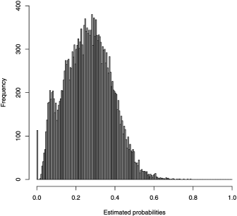
Figure 2: Distribution of estimated probabilities of success.

The interpretation of these probabilities will frequently be subject-specific. Taking into account the economic cost associated with the development of these clusters, the time frame required to develop them, and the potential social and economic gains that they may bring, researchers can define the minimum probability of success that would justify further study.

The analysis of the confidence intervals also offers some important insight. First, although moderately wide, the confidence intervals still allow useful inferences. The large inter-expert heterogeneity may hint at possible measures to increase precision in future studies. Second, using the lower bound of the confidence intervals to rank the clusters, instead of the point estimate of the probability of success, may yield different results. By this criterion, cluster 265222, ranked eighth by the point estimate, would become the second most promising candidate. Clearly, some more fundamental, substantive considerations may be needed to complement the information in Table 1 during the decision-making process.

As a sensitivity analysis we also considered $N_{k}=15$, $W=20$, $S=1468$, with $Q=10\mbox{,}000$. The results appear in the columns labeled “unweighted” in Table 2. Clearly, the differences with the original analysis are negligible.

Table 2: Estimates for the fixed effects and probabilities of success obtained from the weighted and unweighted analyses for the top $20$ clusters in terms of unweighted probability; $\widehat{\beta}_{\mathrm{weighted}}$ and $\widehat{\beta}_{\mathrm{unweighted}}$ are the estimated cluster effects with the ranks in parentheses, and $\widehat{\operatorname{prob}}_{\mathrm{weighted}}$ and $\widehat{\operatorname{prob}}_{\mathrm{unweighted}}$ are the corresponding probabilities of success

ID	$\bolds{\widehat{\beta}_{\mathrm{weighted}}}$	$\bolds{\widehat{\beta}_{\mathrm{{unweighted}}}}$	$\bolds{\widehat{\mathrm{prob}}_{\mathrm{weighted}}}$		$\bolds{\widehat{\mathrm{prob}}_{\mathrm{unweighted}}}$
295061	$3.86$	3.33	0.90	(2)	0.80	(1)
296535	$1.99$	2.71	0.74	(54)	0.76	(2)
84163	$0.86$	2.42	0.61	(376)	0.73	(3)
296443	$0.54$	2.41	0.57	(620)	0.73	(4)
313914	$3.79$	2.37	0.89	(3)	0.73	(5)
265222	$0.56$	2.40	0.57	(653)	0.73	(6)
333529	$1.85$	1.99	0.73	(67)	0.69	(7)
296560	$1.26$	1.91	0.66	(198)	0.69	(8)
178994	$2.25$	1.91	0.77	(28)	0.69	(9)
265441	$1.22$	1.94	0.66	(211)	0.69	(10)
277774	$2.26$	1.87	0.77	(29)	0.69	(11)
292579	$2.69$	1.91	0.81	(10)	0.69	(12)
315928	$1.18$	1.87	0.65	(233)	0.68	(13)
277619	$-0.63$	1.74	0.42	(3165)	0.67	(14)
263047	$3.85$	1.78	0.90	(1)	0.67	(15)
296427	$2.70$	1.65	0.81	(12)	0.67	(16)
292805	$1.00$	1.60	0.63	(313)	0.66	(17)
178828	$2.26$	1.52	0.77	(27)	0.66	(18)
462994	$1.31$	1.46	0.67	(183)	0.65	(19)
159643	$1.93$	1.50	0.74	(55)	0.65	(20)
$\widehat{\sigma}^{2}$	$3.19$	15.80

3.2 Weighted analysis

An important issue discussed in Section 1.1 was the differences encountered in the numbers of clusters evaluated by the experts. One may wonder whether experts who evaluated a large number of clusters gave as careful consideration to each cluster as those who evaluated only a few. Importantly, the model-based approach introduced in Section 2 can take into account these differences by carrying out a weighted analysis, which maximizes the likelihood function

$$L\bigl{(}\bolds{\beta},\sigma^{2}\bigr{)}=\prod_{i=1}^{n}\omega_{i}\int^{\infty}_{-\infty}{\prod_{{j\in\mathchar 259\relax_{i}}}}\pi_{ij}^{y_{ij}}(1-\pi_{ij})^{1-y_{ij}}\phi\bigl{(}b_{i}|0,\sigma^{2}\bigr{)}\,db_{i},$$ (4)

where $\omega_{i}=N/|\mathchar 259\relax_{i}|$ and $|\mathchar 259\relax_{i}|$ denotes the size of $\mathchar 259\relax_{i}$. Practically, a weighted analysis, using the SAS procedure NLMIXED, implies replication of each response vector by $\omega_{i}$, resulting in a pseudo-data set with larger sample size than in the unweighted analysis. Using partitions with $N_{k}=30$ was rather challenging; consequently, the weighted analysis was carried out with $N_{k}=15$. The main results are displayed in Table 2.

Interestingly, some important differences emerge from the two approaches. For instance, the top-ranked cluster in the unweighted analysis received rank 2 in the weighted approach. Some differences are even more dramatic; for example, the fourth cluster in the unweighted analysis received rank 620 in the weighted approach. Clearly, a very careful and thoughtful discussion of these differences will be needed during the decision-making process. In addition, these results also point out the importance of a careful design of the study and may suggest changes in the design to avoid large differences in the numbers of clusters evaluated by the experts. The top 20 in Table 2 is very similar to the one in Table 1, but it is not exactly the same. For example, the cluster ranked 20th is not in Table 1, probably because of the change in $\widehat{\sigma}^{2}$.

Fitting model (1) to the entire data set using maximum likelihood was unfeasible in this case study. Therefore, all previous conclusions were derived by implementing the procedure described in Section 2. One may wonder how the previous procedure would compare with maximum likelihood when the latter is tractable. In the next section we investigate this important issue via simulation.

4 Simulation study

The simulations were designed to mimic the main characteristics encountered in the case study. Two hundred data sets were generated, with the following parameters held constant across data sets: (1) Number of clusters $N=50$, chosen to ensure tractability of maximum likelihood estimation for the whole data, (2) number of experts $n=147$, and (3) a set of 50 values assigned to the parameters characterizing the cluster effects ($\beta_{j}$), which were sampled from a $N(-2,2)$ one time and then held constant in all data sets. Factors varying among the data sets were as follows: (1) the number of ratings per expert $n_{i}$, independently sampled from $\operatorname{Poisson}(25)$ and restricted to the range of 8 to 50, and (2) a set of $147$ expert random effects $b_{i}$, independently sampled from $N(0,12.25$). Conceptually, each generated data set represents a replication of the evaluation study in which a new set of experts rates the same clusters. Therefore, varying $b_{i}$ from one data set to another resembles the use of different groups of experts in each study, sampled from the entire population of experts. Clearly, $n_{i}$ needs to vary simultaneously with $b_{i}$. The probability that expert $i$ would recommend the inclusion of cluster $j$ in the sponsor’s database, $P_{ij}=P(Y_{ij}=1|\beta_{j},b_{i})$, was computed using model (1) and the response $Y_{ij}\sim\operatorname{Bernoulli}(P_{ij})$. Finally, model (1) was fitted using full maximum likelihood and the procedure introduced in Section 2, and their corresponding probabilities of success, given by (3), were compared. Parameters used in the split procedure were $N_{k}=5$, $W=20$, $Q=10\mbox{,}000$ and $S=10$.

The main results of the simulation study for the top $20$ clusters (those with the highest true probability of success) are summarized in Tables 3 and 4. Table 3 clearly shows that the proposed procedure performs as well as maximum likelihood, for the point estimates of the cluster effect. Further, Figure 3 shows that this is true for most of the clusters, as the average relative differences from the true values, for the maximum likelihood estimators [$(\widehat{\beta}_{j,\mathrm{mle}}-\beta_{j})/{\beta_{j}}$] and the estimators obtained from the split procedure [$(\widehat{\beta}_{j,\mathrm{split}}-\beta_{j})/{\beta_{j}}$], are very close to zero most of the time. Interestingly, maximum likelihood cluster-effect estimates for clusters 14, 27, 30 and 32 have a noticeably larger average relative bias than their split-procedure counterparts (#30 is off the scale). This results from the fact that, for these four clusters, the denominator in the relative-difference expression is very small, highlighting a well-known shortcoming of ratios and relative differences. In Table 4, the corresponding values are unremarkable.

Table 3: True value and average parameter estimate for the top $20$ clusters (ID) in the simulation study, estimated from full maximum likelihood (likelihood) and the split procedure (procedure)

	$\bolds{\beta_{j}}$
ID	True	Likelihood	Procedure
3	$2.33$	$2.38$	$2.36$
1	$1.60$	$1.63$	$1.65$
33	$1.52$	$1.56$	$1.54$
47	$1.43$	$1.45$	$1.48$
50	$1.04$	$1.03$	$1.05$
27	$0.13$	$0.07$	$0.11$
30	$0.06$	$0.01$	$0.05$
32	$0.06$	$0.03$	$0.06$
14	$-0.11$	$-0.14$	$-0.11$
7	$-0.30$	$-0.33$	$-0.29$
9	$-0.49$	$-0.50$	$-0.46$
48	$-0.63$	$-0.65$	$-0.61$
10	$-0.71$	$-0.70$	$-0.66$
21	$-0.97$	$-1.00$	$-0.98$
11	$-1.12$	$-1.19$	$-1.14$
26	$-1.13$	$-1.12$	$-1.07$
15	$-1.32$	$-1.33$	$-1.29$
13	$-1.40$	$-1.42$	$-1.38$
4	$-1.42$	$-1.47$	$-1.42$
42	$-1.61$	$-1.69$	$-1.66$
$\widehat{\sigma}^{2}$	$12.25$	$12.96$	$12.74$

Table 4: Average estimated success probabilities for top $20$ clusters (ID) in the simulation study, using full likelihood (lik.) and the split procedure (proc.), percentage of coverage of the confidence intervals (coverage %), percentage of times the true value was less than lower confidence limit [noncov. (above) %], and percentage of times the true value was greater than upper confidence limit [noncoverage (below) %]

		Probability					Noncov.		Noncov.
		of success			Coverage %		(above) %		(below) %
Rank	ID	True	Lik.	Proc.	Lik.	Proc.	Lik.	Proc.	Lik.	Proc.
1	$3$	0.72	0.72	0.73	0.94	0.95	0.02	0.02	0.05	0.04
2	$1$	0.66	0.66	0.66	0.95	0.96	0.03	0.02	0.03	0.03
3	$33$	0.65	0.65	0.65	0.98	0.97	0.01	0.01	0.02	0.02
4	$47$	0.64	0.64	0.65	0.96	0.96	0.02	0.02	0.02	0.02
5	$50$	0.60	0.60	0.61	0.96	0.96	0.02	0.02	0.03	0.01
6	$27$	0.51	0.51	0.51	0.96	0.96	0.02	0.02	0.03	0.02
7	$30$	0.51	0.50	0.51	0.93	0.94	0.03	0.02	0.04	0.03
8	$32$	0.51	0.50	0.51	0.94	0.96	0.04	0.02	0.03	0.01
9	$14$	0.49	0.49	0.49	0.97	0.96	0.01	0.01	0.03	0.03
10	$7$	0.47	0.47	0.47	0.94	0.96	0.01	0.02	0.05	0.02
11	$9$	0.45	0.45	0.45	0.97	0.96	0.02	0.02	0.02	0.02
12	$48$	0.44	0.44	0.44	0.96	0.96	0.03	0.03	0.01	0.01
13	$10$	0.43	0.43	0.43	0.92	0.95	0.04	0.03	0.05	0.03
14	$21$	0.40	0.40	0.40	0.97	0.97	0.02	0.02	0.01	0.01
15	$11$	0.39	0.38	0.39	0.95	0.95	0.03	0.03	0.03	0.02
16	$26$	0.39	0.39	0.39	0.94	0.95	0.04	0.04	0.02	0.01
17	$15$	0.37	0.37	0.37	0.96	0.97	0.03	0.02	0.01	0.01
18	$13$	0.36	0.36	0.36	0.95	0.96	0.04	0.03	0.02	0.02
19	$4$	0.36	0.36	0.36	0.94	0.95	0.03	0.03	0.04	0.02
20	$42$	0.34	0.34	0.34	0.95	0.97	0.04	0.02	0.02	0.01

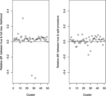
Figure 3: Average relative difference between the true values and the estimates obtained from maximum likelihood, $\frac{\widehat{\beta}_{j,\mathrm{mle}}-\beta_{j}}{\beta_{j}}$ (left) and the split procedure $\frac{\widehat{\beta}_{j,\mathrm{split}}-\beta_{j}}{\beta_{j}}$(right). (Results of the simulation study.)

Further scrutiny of the estimated success probabilities in Table 4 confirms the similarity in performance between the two methods. Here again the point estimates are very close to the true values, and the coverage of the confidence intervals lies around 95% for maximum likelihood as well as for the split procedure. Relative differences between the true values and estimates from the two methods are mostly positive, suggesting that many cluster effects were slightly overestimated. These results further confirm the heuristic conclusions derived in Section 2, stating that the split procedure should often yield results very similar to maximum likelihood when $W$ is sufficiently large.

5 Conclusion

In our quest to quantify expert opinion on the potential of clusters of chemical compounds, we have introduced a permutational-splitting sample procedure. A combination of maximum likelihood estimation, resampling and stochastic methods produced parameter estimates and confidence intervals comparable to those obtained from full maximum likelihood. Loss in precision with the split procedure, apparent in wider confidence intervals, is anticipated, because the procedure splits the data into dependent subsamples, resulting in a less efficient estimate of the random-effect variance.

The model used for the statistical analysis and the conclusions derived from it rest on a number of assumptions, such as the distribution of the expert-specific effect $b_{i}$. Although the normality assumption for the random effects is standard in most software packages, in principle, it would be possible to consider other distributions. For instance, using probability integral transformations in the SAS procedure NLMIXED, other distribution could be fitted, but obtaining convergence is much more challenging with these models [Nelson et al. (2006)].

One could also extend the model by letting the expert effects vary among clusters. However, this extension would dramatically increase the dimension of the vector of random effects, aggravating the already challenging numerical problems. In general, the successful application of the Rasch model in psychometrics to tackle problems similar to the one considered here makes us believe that, although it cannot be formally proven, model (1) may offer a feasible and reliable way to estimate the success probabilities of interest.

More simulation studies and applications to real problems will shed light on the potential and limitations of the model and fitting procedure proposed in the present work. Importantly, their application is possible with commonly available software, and a simulated data set with the corresponding SAS code for the analysis can be freely downloaded from http://www.ibiostat.be/software/.

Even though it was not the focus of the present work, it is clear that the design of the study is another important element to guarantee the validity of the results. Optimal designs are a class of experimental designs that are optimal with respect to some statistical criterion [Berger and Wong (2009)]. For instance, one may aim to select the number of experts, the number of clusters assigned to the experts and the assignment mechanism to maximize precision when estimating the probabilities of success. In principle, it seems intuitively desirable for each cluster to be evaluated by the same number of experts and for each pair of experts to have a reasonable number of clusters in common. However, more research will be needed to clarify these issues and establish the best possible design for this type of study.

References

- Agrafiotis et al. (2007) {barticle}[auto:parserefs-M02] \bauthor\bsnmAgrafiotis, \bfnmD. K.\binitsD. K., \bauthor\bsnmAlex, \bfnmS.\binitsS., \bauthor\bsnmDai, \bfnmH.\binitsH., \bauthor\bsnmDerkinderen, \bfnmA.\binitsA., \bauthor\bsnmFarnum, \bfnmM.\binitsM., \bauthor\bsnmGates, \bfnmP.\binitsP., \bauthor\bsnmIzrailev, \bfnmS.\binitsS., \bauthor\bsnmJaeger, \bfnmE. P.\binitsE. P., \bauthor\bsnmKonstant, \bfnmP.\binitsP., \bauthor\bsnmLeung, \bfnmA.\binitsA., \bauthor\bsnmLobanov, \bfnmV. S.\binitsV. S., \bauthor\bsnmMarichal, \bfnmP.\binitsP., \bauthor\bsnmMartin, \bfnmD.\binitsD., \bauthor\bsnmRassokhin, \bfnmD. N.\binitsD. N., \bauthor\bsnmShemanarev, \bfnmM.\binitsM., \bauthor\bsnmSkalkin, \bfnmA.\binitsA., \bauthor\bsnmStong, \bfnmJ.\binitsJ., \bauthor\bsnmTabruyn, \bfnmT.\binitsT., \bauthor\bsnmVermeiren, \bfnmM.\binitsM., \bauthor\bsnmWan, \bfnmJ.\binitsJ., \bauthor\bsnmXu, \bfnmX. Y.\binitsX. Y. and \bauthor\bsnmYao, \bfnmX.\binitsX. (\byear2007). \btitleAdvanced Biological and Chemical Discovery (ABCD): Centralizing discovery knowledge in an inherently decentralized world. \bjournalJ. Chem. Inf. Model \bvolume47 \bpages1999–2014. \bptokimsref\endbibitem
- Berger and Wong (2009) {bbook}[auto:parserefs-M02] \bauthor\bsnmBerger, \bfnmM.\binitsM. and \bauthor\bsnmWong, \bfnmW.\binitsW. (\byear2009). \btitleAn Introduction to Optimal Designs for Social and Biomedical Research. \bpublisherWiley-Blackwell, \blocationOxford. \bptokimsref\endbibitem
- Birkel (1992) {barticle}[mr] \bauthor\bsnmBirkel, \bfnmThomas\binitsT. (\byear1992). \btitleLaws of large numbers under dependence assumptions. \bjournalStatist. Probab. Lett. \bvolume14 \bpages355–362. \biddoi=10.1016/0167-7152(92)90096-N, issn=0167-7152, mr=1179641 \bptokimsref\endbibitem
- Bond and Fox (2007) {bbook}[auto:parserefs-M02] \bauthor\bsnmBond, \bfnmT. G.\binitsT. G. and \bauthor\bsnmFox, \bfnmC. M.\binitsC. M. (\byear2007). \btitleApplying the Rasch Model: Fundamental Measurement in the Human Sciences, \bedition2nd ed. \bpublisherLawrence Erlbaum, \blocationMahwah, NJ. \bptokimsref\endbibitem
- Chen and Xie (2012) {bmisc}[auto:parserefs-M02] \bauthor\bsnmChen, \bfnmX.\binitsX. and \bauthor\bsnmXie, \bfnmM.\binitsM. (\byear2012). \bhowpublishedA split-and-conquer approach for analysis of extra ordinary large data. DIMACS Technical Report 2012-01 [cited 2013 June 15]. Available at http://dimacs.rutgers.edu/TechnicalReports/TechReports/2012/2012-01.pdf. \bptokimsref\endbibitem
- De Boeck and Wilson (2004) {bbook}[mr] \beditor\bsnmDe Boeck, \bfnmP.\binitsP. and \beditor\bsnmWilson, \bfnmM.\binitsM., eds. (\byear2004). \btitleExplanatory Item Response Models: A Generalized Linear and Nonlinear Approach. \bpublisherSpringer, \blocationNew York. \biddoi=10.1007/978-1-4757-3990-9, mr=2083193 \bptokimsref\endbibitem
- Donoho (2000) {bmisc}[auto:parserefs-M02] \bauthor\bsnmDonoho, \bfnmD. L.\binitsD. L. (\byear2000). \bhowpublishedHigh-dimensional data analysis: The curses and blessings of dimensionality. Aide-Memoire [cited 2013 June 15]. Available at http://www-stat.stanford.edu/~donoho/Lectures/AMS2000/Curses.pdf. \bptokimsref\endbibitem
- Fan, Guo and Hao (2012) {barticle}[mr] \bauthor\bsnmFan, \bfnmJianqing\binitsJ., \bauthor\bsnmGuo, \bfnmShaojun\binitsS. and \bauthor\bsnmHao, \bfnmNing\binitsN. (\byear2012). \btitleVariance estimation using refitted cross-validation in ultrahigh dimensional regression. \bjournalJ. R. Stat. Soc. Ser. B Stat. Methodol. \bvolume74 \bpages37–65. \biddoi=10.1111/j.1467-9868.2011.01005.x, issn=1369-7412, mr=2885839 \bptokimsref\endbibitem
- Fan and Li (2006) {bincollection}[mr] \bauthor\bsnmFan, \bfnmJianqing\binitsJ. and \bauthor\bsnmLi, \bfnmRunze\binitsR. (\byear2006). \btitleStatistical challenges with high dimensionality: Feature selection in knowledge discovery. In \bbooktitleInternational Congress of Mathematicians, Vol. III (\beditor\binitsM.\bfnmM. \bsnmSanz-Sole, \beditor\binitsJ.\bfnmJ. \bsnmSoria, \beditor\binitsJ. L.\bfnmJ. L. \bsnmVarona and \beditor\binitsJ.\bfnmJ. \bsnmVerdera, eds.) \bpages595–622. \bpublisherEur. Math. Soc., \blocationZürich. \bidmr=2275698 \bptokimsref\endbibitem
- Fieuws and Verbeke (2006) {barticle}[mr] \bauthor\bsnmFieuws, \bfnmSteffen\binitsS. and \bauthor\bsnmVerbeke, \bfnmGeert\binitsG. (\byear2006). \btitlePairwise fitting of mixed models for the joint modeling of multivariate longitudinal profiles. \bjournalBiometrics \bvolume62 \bpages424–431. \biddoi=10.1111/j.1541-0420.2006.00507.x, issn=0006-341X, mr=2227490 \bptokimsref\endbibitem
- Hack et al. (2011) {barticle}[pbm] \bauthor\bsnmHack, \bfnmMichael D.\binitsM. D., \bauthor\bsnmRassokhin, \bfnmDmitrii N.\binitsD. N., \bauthor\bsnmBuyck, \bfnmChristophe\binitsC., \bauthor\bsnmSeierstad, \bfnmMark\binitsM., \bauthor\bsnmSkalkin, \bfnmAndrew\binitsA., \bauthor\bsnmten Holte, \bfnmPeter\binitsP., \bauthor\bsnmJones, \bfnmTodd K.\binitsT. K., \bauthor\bsnmMirzadegan, \bfnmTaraneh\binitsT. and \bauthor\bsnmAgrafiotis, \bfnmDimitris K.\binitsD. K. (\byear2011). \btitleLibrary enhancement through the wisdom of crowds. \bjournalJ. Chem. Inf. Model \bvolume51 \bpages3275–3286. \biddoi=10.1021/ci200446y, issn=1549-960X, pmid=22035213 \bptokimsref\endbibitem
- Johnson and Wichern (2007) {bbook}[mr] \bauthor\bsnmJohnson, \bfnmRichard A.\binitsR. A. and \bauthor\bsnmWichern, \bfnmDean W.\binitsD. W. (\byear2007). \btitleApplied Multivariate Statistical Analysis, \bedition6th ed. \bpublisherPearson Prentice Hall, \blocationUpper Saddle River, NJ. \bidmr=2372475 \bptokimsref\endbibitem
- Li (1991) {barticle}[mr] \bauthor\bsnmLi, \bfnmKer-Chau\binitsK.-C. (\byear1991). \btitleSliced inverse regression for dimension reduction. \bjournalJ. Amer. Statist. Assoc. \bvolume86 \bpages316–342. \bidissn=0162-1459, mr=1137117 \bptnotecheck related \bptokimsref\endbibitem
- Molenberghs and Verbeke (2005) {bbook}[mr] \bauthor\bsnmMolenberghs, \bfnmGeert\binitsG. and \bauthor\bsnmVerbeke, \bfnmGeert\binitsG. (\byear2005). \btitleModels for Discrete Longitudinal Data. \bpublisherSpringer, \blocationNew York. \bidmr=2171048 \bptokimsref\endbibitem
- Molenberghs, Verbeke and Iddi (2011) {barticle}[mr] \bauthor\bsnmMolenberghs, \bfnmGeert\binitsG., \bauthor\bsnmVerbeke, \bfnmGeert\binitsG. and \bauthor\bsnmIddi, \bfnmSamuel\binitsS. (\byear2011). \btitlePseudo-likelihood methodology for partitioned large and complex samples. \bjournalStatist. Probab. Lett. \bvolume81 \bpages892–901. \biddoi=10.1016/j.spl.2011.01.012, issn=0167-7152, mr=2793758 \bptokimsref\endbibitem
- Nelson et al. (2006) {barticle}[mr] \bauthor\bsnmNelson, \bfnmKerrie P.\binitsK. P., \bauthor\bsnmLipsitz, \bfnmStuart R.\binitsS. R., \bauthor\bsnmFitzmaurice, \bfnmGarrett M.\binitsG. M., \bauthor\bsnmIbrahim, \bfnmJoseph\binitsJ., \bauthor\bsnmParzen, \bfnmMichael\binitsM. and \bauthor\bsnmStrawderman, \bfnmRobert\binitsR. (\byear2006). \btitleUse of the probability integral transformation to fit nonlinear mixed-effects models with nonnormal random effects. \bjournalJ. Comput. Graph. Statist. \bvolume15 \bpages39–57. \biddoi=10.1198/106186006X96854, issn=1061-8600, mr=2269362 \bptokimsref\endbibitem
- Newman (1984) {bincollection}[mr] \bauthor\bsnmNewman, \bfnmCharles M.\binitsC. M. (\byear1984). \btitleAsymptotic independence and limit theorems for positively and negatively dependent random variables. In \bbooktitleInequalities in Statistics and Probability (Lincoln, Neb., 1982). \bseriesInstitute of Mathematical Statistics Lecture Notes—Monograph Series \bvolume5 \bpages127–140. \bpublisherIMS, \blocationHayward, CA. \biddoi=10.1214/lnms/1215465639, mr=0789244 \bptokimsref\endbibitem
- Oxman, Lavis and Fretheim (2007) {barticle}[pbm] \bauthor\bsnmOxman, \bfnmAndrew D.\binitsA. D., \bauthor\bsnmLavis, \bfnmJohn N.\binitsJ. N. and \bauthor\bsnmFretheim, \bfnmAtle\binitsA. (\byear2007). \btitleUse of evidence in WHO recommendations. \bjournalLancet \bvolume369 \bpages1883–1889. \biddoi=10.1016/S0140-6736(07)60675-8, issn=1474-547X, pii=S0140-6736(07)60675-8, pmid=17493676 \bptokimsref\endbibitem
- Pinheiro and Bates (1995) {barticle}[auto:parserefs-M02] \bauthor\bsnmPinheiro, \bfnmJ. C.\binitsJ. C. and \bauthor\bsnmBates, \bfnmD. M.\binitsD. M. (\byear1995). \btitleApproximations to the log-likelihood function in the nonlinear mixed-effects model. \bjournalJ. Comput. Graph. Statist. \bvolume4 \bpages12–35. \bptokimsref\endbibitem
- Tibshirani (1996) {barticle}[mr] \bauthor\bsnmTibshirani, \bfnmRobert\binitsR. (\byear1996). \btitleRegression shrinkage and selection via the lasso. \bjournalJ. R. Stat. Soc. Ser. B Stat. Methodol. \bvolume58 \bpages267–288. \bidissn=0035-9246, mr=1379242 \bptokimsref\endbibitem
- Xia et al. (2002) {barticle}[mr] \bauthor\bsnmXia, \bfnmYingcun\binitsY., \bauthor\bsnmTong, \bfnmHowell\binitsH., \bauthor\bsnmLi, \bfnmW. K.\binitsW. K. and \bauthor\bsnmZhu, \bfnmLi-Xing\binitsL.-X. (\byear2002). \btitleAn adaptive estimation of dimension reduction space. \bjournalJ. R. Stat. Soc. Ser. B Stat. Methodol. \bvolume64 \bpages363–410. \biddoi=10.1111/1467-9868.03411, issn=1369-7412, mr=1924297 \bptokimsref\endbibitem