Beyond Pixels: A Comprehensive Survey from Bottom-up to Semantic Image Segmentation and Cosegmentation

Abstract

Image segmentation refers to the process to divide an image into  non-overlapping meaningful regions according to human perception, which has become a classic topic since the early ages of computer vision. A lot of research has been conducted and has resulted in many applications. However, while many segmentation algorithms exist, yet there are only a few sparse and outdated summarizations available, an overview of the recent achievements and issues is lacking. We aim to provide a comprehensive review of the recent progress in this field. Covering 180 publications, we give an overview of broad areas of segmentation topics including not only the classic bottom-up approaches, but also the recent development in superpixel, interactive methods, object proposals, semantic image parsing and image cosegmentation. In addition, we also review the existing influential datasets and evaluation metrics. Finally, we suggest some design flavors and research directions for future research in image segmentation.

1 Introduction

Human can quickly localize many patterns and automatically group them into meaningful parts. Perceptual grouping refers to human’s visual ability to abstract high level information from low level image primitives without any specific knowledge of the image content. Discovering the working mechanisms under this ability has long been studied by the cognitive scientists since 1920’s. Early gestalt psychologists observed that human visual system tends to perceive the configurational whole with rules governing the psychological grouping. The hierarchical grouping from low-level features to high level structures has been proposed by gestalt psychologists which embodies the concept of grouping by proximity, similarity, continuation, closure and symmetry. The highly compact representation of images produced by perceptual grouping can greatly facilitate the subsequent indexing, retrieving and processing.

With the development of modern computer, computer scientists ambitiously want to equip the computer with the perceptual grouping ability given many promising applications, which lays down the foundation for image segmentation, and has been a classical topic since early years of computer vision. Image segmentation, as a basic operation in computer vision, refers to the process to divide a natural image into $K$ non-overlapped meaningful entities (e.g., objects or parts). The segmentation operation has been proved quite useful in many image processing and computer vision tasks. For example, image segmentation has been applied in image annotation [1] by decomposing an image into several blobs corresponding to objects. Superpixel segmentation, which transforms millions of pixels into hundreds or thousands of homogeneous regions [2, 3], has been applied to reduce the model complexity and improve speed and accuracy of some complex vision tasks, such as estimating dense correspondence field [4], scene parsing [5] and body model estimation [6]. [7, 8, 9] have used segmented regions to facilitate object recognition, which provides better localization than sliding windows. The techniques developed in image segmentation, such as Mean Shift [3] and Normalized Cut [10] have also been widely used in other areas such as data clustering and density estimation.

One would expect a segmentation algorithm to decompose an image into the “objects” or semantic/meaningful parts. However, what makes an “object” or a “meaningful” part can be ambiguous. An “object” can be referred to a “thing” (a cup, a cow, etc), a kind of texture (wood, rock) or even a “stuff” (a building or a forest). Sometimes, an “object” can also be part of other “objects”. Lacking a clear definition of “object” makes bottom-up segmentation a challenging and ill-posed problem. Fig. 1 gives an example, where different human subjects have different ways in interpreting objects. In this sense, what makes a ‘good’ segmentation needs to be properly defined.

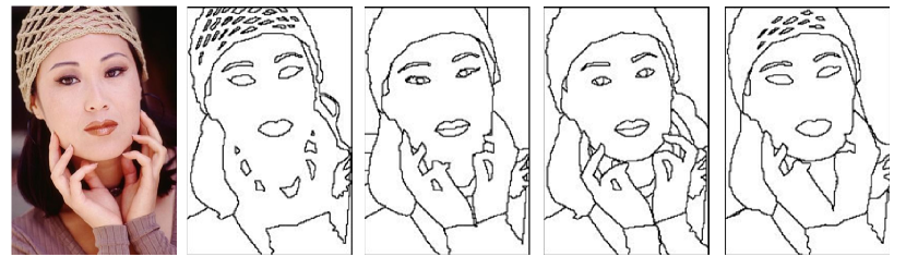
Figure 1: An image from Berkeley segmentation dataset [11] with hand labels from different human subjects, which demonstrates the variety of human perception.

Research in human perception has provided some useful guidelines for developing segmentation algorithms. For example, cognition study [12] shows that human vision views part boundaries at those with negative minima of curvature and the part salience depends on three factors: the relative size, the boundary strength and the degree of protrusion. Gestalt theory and other psychological studies have also developed various principles reflecting human perception, which include: (1) human tends to group elements which have similarities in color, shape or other properties; (2) human favors linking contours whenever the elements of the pattern establish an implied direction.

Another challenge which makes “object” segmentation difficult is how to effectively represent the “object”. When human perceives an image, elements in the brain will be perceived as a whole, but most images in computers are currently represented based on low-level features such as color, texture, curvature, convexity, etc. Such low-level features reflect local properties, which are difficult to capture global object information. They are also sensitive to lighting and perspective variations, which could cause existing algorithms to over-segment the image into trivial regions. Fully supervised methods can learn higher level and global cues, but they can only handle limited number object classes and require per-class labeling.

A lot of research has been conducted on image segmentation. Unsupervised segmentation, as one classic topic in computer vision, has been studied since 70’s. Early techniques focus on local region merging and splitting [13, 14], which borrow ideas from clustering area. Recent techniques, on the other hand, seek to optimize some global criteria [3, 15, 10, 16, 17, 18, 19]. Interactive segmentation methods [20, 21, 22] which utilize user input, have been applied in some commercial products such as Microsoft Office and Adobe Photoshop. The substantial development of image classification [23], object detection [24], superpixel segmentation [2] and 3D scene recovery [25] in the past few years have boosted the research in supervised scene parsing [26, 27, 28, 29, 30, 31]. With the emergence of large-scale image databases, such as the ImageNet [32] and personal photo streams on Flickr, the cosegmentation methods [33, 34, 35, 36, 37, 38, 39, 40] which can extract recurring objects from a set of images, has attracted increasing attentions in these years.

Although image segmentation as a community has been evolving for a long time, the challenges ranging from feature representation to model design and optimization are still not fully resolved, which hinder further performance improvement towards human perception. Thus, it is necessary to periodically give a thorough and systematic review of the segmentation algorithms, especially the recent ones, to summarize what have been achieved, where we are now, what knowledge and lessons can be shared and transferred between different communities and what are the directions and opportunities for future research. To our surprise, there are only some sparse reviews on segmentation literature, there is no comprehensive review which covers broad areas of segmentation topics including not only the classic bottom-up approaches, but also the recent development in superpixel, interactive methods, object proposals, semantic image parsing and image cosegmentation, which will be critically and exhaustively reviewed in this paper in Sections 2-7. In addition, we will also review the existing influential datasets and evaluation metrics in Section 8. Finally, we discuss some popular design flavors and some potential future directions in Section 9, and conclude the paper in Section 10.

2 Bottom-up methods

The bottom-up methods usually do not take into account the explicit notion of the object, and their goal is mainly to group nearby pixels according to some local homogeneity in the feature space, e.g. color, texture or curvature, by clustering those features based on fitting mixture models, mode shifting [3] or graph partitioning [15] [10][16][17]. In addition, the variational [18] and level set [19] techniques have also been used in segmenting images into regions. Below we give a brief summary of some popular bottom-up methods due to their reasonable performance and publicly available implementation. We divide the bottom-up methods into two major categories: discrete methods and continues methods, where the former considers an image as a fixed discrete grid while the latter treats an image as a continuous surface.

2.1 Discrete bottom-up methods

K-Means: K-means is among the simplest and most efficient method. Given $k$ initial centers which can be randomly selected, K-means first assign each sample to one of the centers based on their feature space distance and then the centers are updated. These two steps iterate until the termination condition is met. Assuming that cluster number is known or the distributions of the clusters are spherically symmetric, K-means works efficiently. However, these assumptions often don’t meet in general cases, and thus K-means could have problems when dealing with complex clusters.

Mixture of Gaussians: This method and K-means are similar to each other. Within mixture of Gaussians, each cluster center is now replaced by a covariance matrix. Assume a set of $d$-dimensional feature vector $x_{1},x_{2},...,x_{n}$ which are drawn from a Gaussian mixture:

$$p(x|\{\pi_{k},\mu_{k},\Sigma_{k}\})=\sum_{k}\pi_{k}N(x|\mu_{k},\Sigma_{k})$$ (1)

where $\pi_{k}$ are the mixing weights, $\mu_{k},\Sigma_{k}$ are the means and covariances, and

$$N(x|\mu_{k},\Sigma_{k})=\frac{exp\{-\frac{1}{2}(x-\mu_{k})^{T}\Sigma_{k}^{-1}(x-\mu_{k})\}}{(2\pi)^{d/2}|\Sigma_{k}|^{1/2}}$$ (2)

is the normal equation [41]. The parameters $\pi_{k},\mu_{k},\Sigma_{k}$ can be estimated by using expectation maximization (EM) algorithm as follows [41].

1. The E-step estimates how likely a sample $x_{i}$ is generated from the $k$th Gaussian clusters with current parameters:

   $$z_{ik}=\frac{1}{Z}N(x_{i}|\mu_{k},\Sigma_{k})$$ (3)

   with $\sum_{k}z_{ik}=1$ and $Z=\sum_{k}N(x_{i}|\mu_{k},\Sigma_{k})$.

2. The M-step updates the parameters:

   $$\begin{split}&\mu_{k}=\frac{1}{n_{k}}\sum_{i}z_{ik}x_{i},\\ &\Sigma_{k}=\frac{1}{n_{k}}z_{ik}(x_{i}-\mu_{k})(x_{i}-\mu_{k})^{T},\\ &\pi_{k}=\frac{n_{k}}{n}\end{split}$$ (4)

   where $n_{k}=\sum_{i}z_{ik}$ estimates the number of sample points in each cluster.

After the parameters are estimated, the segmentation can be formed by assigning the pixels to the most probable cluster. Recently, Rao et al [42] extended the gaussian mixture models by encoding the texture and boundary using minimum description length theory and achieved better performance.

Mean Shift: Different from the parametric methods such as K-means and Mixture of Gaussian which have assumptions over the cluster number and feature distributions, Mean-shift [3] is a non-parametric method which can automatically decide the cluster number and modes in the feature space.

Assume the data points are drawn from some probability function, whose density can be estimated by convolving the data with a fixed kernel of width $h$:

$$f(x)=\sum_{i}K(x-x_{i})=\sum_{i}k(\frac{||x-x_{i}||^{2}}{h^{2}})$$ (5)

where $x_{i}$ is an input sample and $k(.)$ is the kernel function [41]. After the density function is estimated, mean shift uses a multiple restart gradient descent method which starts at some initial guess $y_{k}$, then the gradient direction of $f(x)$ is estimated at $y_{k}$ and uphill step is taken in the direction [41]. Particularly, the gradient of $f(x)$ is given by

$$\begin{split}\nabla f(x)&=\sum_{i}(x_{i}-x)G(x-x_{i})\\ &=\sum_{i}(x_{i}-x)g(\frac{||x-x_{i}||^{2}}{h^{2}})\end{split}$$ (6)

where

$$g(r)=-k^{\prime}(r)$$ (7)

and $k^{\prime}(.)$ is the first-order derivative of $k(.)$. $\nabla f(x)$ can be re-written as

$$\nabla f(x)=\left[\sum_{i}G(x-x_{i})\right]m(x)$$ (8)

where the vector

$$m(x)=\frac{\sum_{i}x_{i}G(x-x_{i})}{\sum_{i}G(x-x_{i})}-x$$ (9)

is called the mean shift vector which is the difference between the mean of the neighbors around $x$ and the current value of $x$. During the mean-shift procedure, the current mode $y_{k}$ is replaced by its locally weighted mean:

$$y_{k+1}=y_{k}+m(y_{k}).$$ (10)

Final segmentation is formed by grouping pixels whose converge points are closer than $h_{s}$ in the spatial domain and $h_{r}$ in the range domain, and these two parameters are tuned according to the requirement of different applications.

Watershed: This method [16] segments an image into the catchment and basin by flooding the morphological surface at the local minimum and then constructing ridges at the places where different components meet. As watershed associates each region with a local minimum, it can lead to serious over-segmentation. To mitigate this problem, some methods [17] allow user to provide some initial seed positions which helps improve the result.

Graph Based Region Merging: Unlike edge based region merging methods which use fixed merging rules, Felzenszwalb and Huttenlocher [15] advocates a method which can use a relative dissimilar measure to produce segmentation which optimizes a global grouping metric. The method maps an image to a graph with a $4$-neighbor or $8$-neighbor structure. The pixels denote the nodes, while the edge weights reflect the color dissimilarity between nodes. Initially each node forms their own component. The internal difference $Int(C)$ is defined as the largest weight in the minimum spanning tree of a component $C$. Then the weight is sorted in ascending order. Two regions $C_{1}$ and $C_{2}$ are merged if the in-between edge weight is less than $min(Int(C_{1})+\tau(C_{1}),Int(C_{2})+\tau(C_{2}))$, where $\tau(C)=k/|C|$ and $k$ is a coefficient that is used to control the component size. Merging stops when the difference between components exceeds the internal difference.

Normalized Cut: Many methods generate the segmentation based on local image statistics only, and thus they could produce trivial regions because the low level features are sensitive to the lighting and perspective changes. In contrast, Normalized Cut [43] finds a segmentation via splitting the affinity graph which encodes the global image information, i.e. minimizing the Ncut value between different clusters:

$$Ncut(S_{1},S_{2},...,S_{k}):=\frac{1}{2}\sum_{i=1}^{k}\frac{W(S_{i},\bar{S_{i}})}{vol(S_{i})}$$ (11)

where $S_{1},S_{2},...,S_{k}$ form a $k$-partition of a graph, $\bar{S_{i}}$ is the complement of $S_{i}$, $W(S_{i},\bar{S_{i}})$ is the sum of boundary edge weights of $S_{i}$, and $vol(S_{i})$ is the sum of weights of all edges attached to vertices in $S_{i}$. The basic idea here is that big clusters have large $vol(S_{i})$ and minimizing Ncut encourages all $vol(S_{i})$ to be about the same, thus achieving a “balanced” clustering.

Finding the normalized cut is an NP-hard problem. Usually, an approximate solution is sought by computing the eigenvectors $v$ of the generalized eigenvalue system $(D-W)v=\lambda Dv$, where $W=[w_{ij}]$ is the affinity matrix of an image graph with $w_{ij}$ describing the pairwise affinity of two pixels and $D=[d_{ij}]$ is the diagonal matrix with $d_{ii}=\sum_{j}w_{ij}$. In the seminal work of Shi and Malik [43], the pair-wise affinity is chosen as the Gaussian kernel of the spatial and feature difference for pixels within a radius $||x_{i}-x_{j}||<r$:

$$W_{ij}=exp(-\frac{||F_{i}-F_{j}||^{2}}{\sigma_{F}^{2}}-\frac{||x_{i}-x_{j}||^{2}}{\sigma_{s}^{2}})$$ (12)

where $F$ is a feature vector consisting of intensity, color and Gabor features and $\sigma_{F}$ and $\sigma_{s}$ are the variance of the feature and spatial position, respectively. In the later work of Malik et al. [44], they define a new affinity matrix using an intervening contour method. They measure the difference between two pixel $i$ and $j$ by inspecting the probability of an obvious edge alone the line connecting the two pixels:

$$W_{ij}=exp(-\max_{p\in\bar{ij}}{~{}mPb(p)}/\sigma)$$ (13)

where $\bar{ij}$ is the line segment connecting $i$ and $j$ and $\sigma$ is a constant, the $mPb(p)$ is the boundary strength defined at pixel $p$ by maximizing the oriented contour signal $mPb(p,\theta)$ at multiple orientations $\theta$ :

$$mPb(p)=\max_{\theta}~{}{mPb(p,\theta)}$$ (14)

The oriented contour signal $mPb(p,\theta)$ is defined as a linear cobination of multiple local cuess at orientation $\theta$:

$$mPb(p,\theta)=\sum_{s}\sum_{i}\alpha_{i,s}G_{i,\sigma(i,s)}(p,\theta)$$ (15)

where $G_{i,\sigma(i,s)}(p,\theta)$ measures the $\chi^{2}$ distance at feature channel $i$ (brightness, color a, color b, texture) between the histograms of the two halves of a disc of radius $\sigma(i,s)$ divided at angle $\theta$, and $\alpha_{i,s}$ is the combination weight by gradient ascent on the F-measure using the training images and corresponding ground-truth. Moreover, the affinity matrix can also be learned by using the recent multi-task low-rank representation algorithm presented in [45].

The segmentation is achieved by recursively bi-partitioning the graph using the first nonzero eigenvalue’s eigenvector [10] or spectral clustering of a set of eigenvectors [46]. For the computational efficiency purpose, spectral clustering requires the affinity matrix to be sparse which limits its applications. Recent work of Cour et al. [47] solves this limitation by defining the affinity matrix at multiple scale and then setting up cross-scale constraints which achieve better result. In addition, Arbelaez et al. [48] convolve eigenvectors with Gaussian directional derivatives at multiple orientations $\theta$ to obtain oriented spectral contours responses at each pixel $p$:

$$sPb(p,~{}\theta)=\sum\limits_{k=1}^{n}\frac{1}{\sqrt{\lambda_{k}}}\cdot\triangledown_{\theta}\textbf{v}_{k}(p)$$ (16)

Since the signal $mPb$ and $sPb$ carries different contour information, Arbelaez et al. [48] proposed to combine them to globalized the contour information $gPb$:

$$gPb(p,\theta)=\beta\cdot mPb(p,\theta)+\gamma\cdot sPb(p,\theta)$$ (17)

where the combination weights $\beta$ and $\gamma$ are also learned by gradient ascent on the F-measure using ground truth, which achieved the state-of-the-art contour detection result.

Edge Based Region Merging: Such methods [14][49] start from pixels or super-pixels, and then two adjacent regions are merged based on the metrics which can reflect their similarities/dissimilarities such as boundary length, edge strength or color difference. Recently, Arbelaez et al. [50] proposed the gPb-OWT-UCM method to transform a set of contours, which are generated from the Normalized Cut framework (to be introduced later), into a nested partition of the image. The method first generate a probability edge map $gPb$ (see Eq.17) which delineates the salient contours. Then, it performs watershed over the topological space defined by the $gPb$ to form the finest level segmentation. Finally, the edges between regions are sorted and merged in an ascending order which forms the ultrametric contour map $UCM$. Thresholding $UCM$ at a scale $\lambda$ forms the final segmentation.

2.2 Continuous methods

Variational techniques [19, 18, 51, 52, 53] have also been used in segmenting images into regions, which treat an image as a continuous surface instead of a fixed discrete grid and can produce visually more pleasing results.

Mumford-Shah Model: The Mumford-Shah (MS) model partitions an image by minimizing the functional which encourages homogeneity within each region as well as sharp piecewise regular boundaries. The MS functional is defined as

$$F_{MS}(I,C)=\int_{\omega}|I-I_{0}|^{2}dx+\mu\int_{\omega\backslash C}|\nabla I|^{2}dx+\nu H^{N-1}(C)$$ (18)

for any observed image $I_{0}$ and any positive parameters $\mu,\nu$, where $I$ corresponds to a piecewise smooth approximation of $I_{0}$, $C$ represents the boundary contours of $I$ and its length is given by Hausdorff measure $H^{N-1}(C)$. The first term of (18) is a fidelity term with respect to the given data $I_{0}$, the second term regularizes the function $I$ to be smooth inside the region $\omega\backslash C$ and the last term imposes a regularization constraint on the discontinuity set $C$ to be smooth.

Since minimizing the Mumford-Shah model is not easy, many variants have been proposed to approximate the functional [54, 55, 56, 57]. Among them, Vese-Chan[58] proposed to approximate the term $H^{N-1}(C)$ by the lengths of region contours, which provides the model of active contour without edges. By assuming the region is piecewise constant, the model is further simplified to the continuous Potts model, which has convexified solvers [52, 53].

Active Contour / Snake Model [59]: This type of models detects objects by deforming a snake/contour curve $C$ towards the sharp image edges. The evolution of parametric curve $C(p)=(x(p),y(p)),p\in\{0,1\}$ is driven by minimizing the functional:

$$F(C)=\alpha\int_{0}^{1}|\frac{\partial C(p)}{\partial p}|^{2}dp+\beta\int_{0}^{1}|\frac{\partial^{2}C}{\partial p^{2}}|^{2}dp+\lambda\int_{0}^{1}f^{2}(I_{0}(C))dp$$ (19)

where the first two terms enforce smoothness constraints by making the snake act as a membrane and a thin plate correspondingly, and the sum of the first two terms makes the internal energy. The third term, called external energy, attracts the curve toward the object boundaries by using the edge detecting function

$$f(I_{0})=\frac{1}{1+\gamma|\nabla(I_{0}*G_{\sigma})|^{2}}$$ (20)

where $\gamma$ is an arbitrary positive constant and $I_{0}*G_{\sigma}$ is the Gaussian smoothed version of $I_{0}$. The energy function is non-convex and sensitive to initialization. To overcome the limitation, Osher et al. [19] proposed the level set method, which implicitly represents curve $C$ by a higher dimension $\psi$, called the level set function. Moreover, Bresson et al. [51] proposed the convex relaxed active contour model which can achieve desirable global optimal.

The bottom-up methods can also be classified into another two categories: the ones [15][10][50] which attempt to produce regions likely belonging to objects and the ones which tend to produce over-segmentation [16][3] (to be introduced in Section 3). For methods of the first category, obtaining object regions is extremely challenging as the bottom-up methods only use low-level features. Recently, Zhu et al. [60] proposed to combine hand-crafted low-level features that can reflect global image statistics (such as Gaussian Mixture Model, Geodesic Distance and Eigenvectors) with the convexified continuous Potts model to capture high-level structures, which achieves some promising results.

3 Superpixel

Superpixel methods aim to over-segment an image into homogeneous regions which are smaller than object or parts. In the seminal work of Ren and Malik [61], they argue and justify that superpixel is more natural and efficient representation than pixel because local cues extracted at pixel are ambiguous and sensitive to noise. Superpixel has a few desirable properties:

• It is perceptually more meaningful than pixel. The superpixel produced by state-of-the-art algorithms is nearly perceptually consistent in terms of color, texture, etc, and most structures can be well preserved. Besides, superpixel also conveys some shape cues which is difficult to capture at pixel level.

• It helps reduce model complexity and improve efficiency and accuracy. Existing pixel-based methods need to deal with millions of pixels and their parameters, where training and inference in such a big system pose great challenges to current solvers. On the contrary, using superpixels to represent the image can greatly reduce the number of parameters and alleviate computation cost. Meanwhile, by exploiting the large spatial support of superpixel, more discriminative features such as color or texture histogram can be extracted. Last but not least, superpixel makes longer range information propagation possible, which allows existing solvers to exploit richer information than those using pixel.

There are different paradigms to produce superpixels:

• Some existing bottom-up methods can be directly adapted to over-segmentation scenario by tuning the parameters, e.g. Watersheds, Normalized Cut (by increasing cluster number), Graph Based Merging (by controlling the regions size) and Mean-Shift/Quick-Shift (by tuning the kernel size or changing mode drifting style).

• Some recent methods produce much faster superpixel segmentation by changing optimization scope from the whole image to local non-overlap initial regions, and then adjusting the region boundaries to snap to salient object contours. TurboPixel [62] deforms the initial spatial grid to compact and regular regions by using geometric flow which is directed by local gradients. Wang et al. [63] also adapted geodesic flows by computing geodesic distance among pixels to produce adaptive superpixels, which have higher density in high intensity or color variation regions while having larger superpixels at structure-less regions. Veskler et al. [64] proposed to place overlapping patches at the image, and then assigned each pixel by inferring the MAP solution using graph-cuts. Zhang et al. [65] further studied in this direction by using a pseudo-boolean optimization which achieves faster speed. Achanta et al. [2] introduced the SLIC algorithm which greatly improves the superpixel efficiency. SLIC starts from the initial regular grid of superpixels, grows superpixels by estimating each pixel’s distance to its cluster center localized nearby, and then updates the cluster centers, which is essentially a localized K-means. SLIC can produce superpixels at 5Hz without GPU optimization.

• There are also some new formulations for over-segmentation. Liu et al. [66] recently proposed a new graph based method, which can maximize the entropy rate of the cuts in the graph with a balance term for compact representation. Although it outperforms many methods in terms of boundary recall measure, it takes about 2.5s to segment an image of size 480x320. Van den Berge et al. [67] proposed the fastest superpixel method-SEED, which can run at 30Hz. SEED uses multi-resolution image grids as initial regions. For each image grid, they define a color histogram based entropy term and an optional boundary term. Instead of using EM as in SLIC, which needs to repeatedly compute distances, SEEDs uses Hill-Climbing to move coarser-resolution grids, and then refines region boundary using finer-resolution grids. In this way, SEEDs can achieve real time superpixel segmentation at 30Hz.

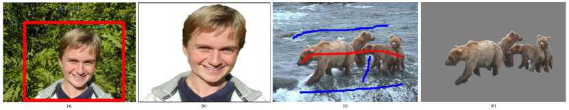
Figure 2: Examples of interactive image segmentation using bounding box (a $\sim$ b) [20] or scribbles (c $\sim$ d) [21].

4 Interactive methods

Image segmentation is expected to produce regions matching human perception. Without any prior assumption, it is difficult for bottom-up methods to produce object regions. For some specific areas such as image editing and medical image analysis, which require precise object localization and segmentation for subsequent applications (e.g. changing background or organ reconstruction), prior knowledge or constraints (e.g. color distribution, contour enclosure or texture distribution) directly obtained from a small amount of user inputs can be of great help to produce accurate object segmentation. Such type of segmentation methods with user inputs are termed as interactive image segmentation methods. There are already some surveys [68, 69, 70] on interactive segmentation techniques, and thus this paper will act as a supplementary to them, where we discuss recent influential literature not covered by the previous surveys. In addition, to make the manuscript self-contained, we will also give a brief review of some classical techniques.

In general, an interactive segmentation method has the following pipeline: 1) user provides initial input; 2) then segmentation algorithm produces segmentation results; 3) based on the results, user provides further constraints, and then go back to step 2. The process repeats until the results are satisfactory. A good interactive segmentation method should meet the following criteria: 1) offering an intuitive interface for the user to express various constraints; 2) producing fast and accurate result with as little user manipulation as possible; 3) allowing user to make additional adjustments to further refine the result.

Existing interactive methods can be classified according to the difference of the user interface, which is the bridge for the user to convey his prior knowledge (see Fig. 2). Existing popular interfaces include bounding box [20], polygon (the object of interest is within the provided regions), contour [71, 72] (the object boundary should follow the provided direction), and scribbles [73, 21] (the object should follow similar color distributions). According to the methodology, the existing interactive methods can be roughly classified into two groups: (i) contour based methods and (ii) label propagation based methods [70].

4.1 Contour based interactive methods

Contour based methods are one type of the earliest interactive segmentation methods. In a typical contour based interactive method, the user first places a contour close to the object boundary, and then the contour will evolve to snap to the nearby salient object boundary. One of the key components for contour based methods is the edge detection function, which can be based on first-order image statistics (such as operators of Sobel, Canny, Prewitt, etc), or more robust second-order statistics (such as operators of Laplacian, LoG, etc).

For instance, the Live-Wire / Intelligent Scissors method [72, 74] starts contour evolving by building a weighted graph on the image, where each node in the graph corresponds to a pixel, and directed edges are formed around pixels with their closest four neighbors or eight neighbors. The local cost of each direct edge is the weighted sum of Laplacian zero-cross, gradient magnitude and gradient direction. Then given the seed locations, the shortest path from a seed point $p$ to a certain seed point $s$ is found by using Dijikstra’s method. Essentially, Live-Wire minimizes a local energy function. On the other hand, the active contour method introduced in Section 2.2 deforms the contour by using a global energy function, which consists of a regional term and a boundary term, to overcome some ambiguous local optimum. Nguyen et al. [22] recently employed the convex active contour model to refine the object boundary produced by other interactive segmentation methods and achieved satisfactory segmentation results. Liu et al. [75] proposed to use the level set function [19] to track the zero level set of the posterior probabilistic mask learned from the user provided bounding box, which can capture objects with complex topology and fragmented appearance such as tree leaves.

4.2 Label propagation based methods

Label Propagation methods are more popular in literature. The basic idea of label propagation is to start from user-provided initial input marks, and then propagate the labels using either global optimization (such as GraphCut [73] or RandomWalk [76]) or local optimization, where the global optimization methods are more widely used due to the existence of fast solvers.

GraphCut and its decedents [73, 20, 77] model the pixel labeling problem in Markov Random Field. Their energy functions can be generally expressed as

$$E(X)=\sum_{x_{i}\in X}E_{u}(x_{i})+\sum_{x_{i},x_{j}\in\cal{N}}E_{p}(x_{i},x_{j})$$ (21)

where $X={x_{1},x_{2},...,x_{n}}$ is the set of random variables defined at each pixel, which can take either foreground label $1$ or background label $0$; $\cal{N}$ defines a neighborhood system, which is typically 4-neighbor or 8-neighbor. The first term in (21) is the unary potential, and the second term is the pairwise potential. In [73], the unary potential is evaluated by using an intensity histogram. Later in GrabCut [20], the unary potential is derived from the two Gaussian Mixture Models (GMMs) for background and foreground regions respectively, and then a hard constraint is imposed on the regions outside the bounding box such that the labels in the background region remain constant while the regions within the box are updated to capture the object. Li et al. [77] further proposed the LazySnap method, which extends GrabCut by using superpixels and including an interface to allow user to adjust the result at the low-contrast and weak object boundaries. One limitation of GrabCut is that it favors short boundary due to the energy function design. Recently Kohli et al. [78] proposed to use a conditional random field with multiple-layered hidden units to encode boundary preserving higher order potential, which has efficient solvers and therefore can capture thin details that are often neglected by classical MRF model.

Since MRF/CRF model provides a unified framework to combine multiple information, various methods have been proposed to incorporate prior knowledge:

• Geodesic prior: One typical assumption on objects is that they are compactly clustered in spatial space, instead of distributing around. Such spatial constraint can be constructed by exploiting the geodesic distance to foreground and background seeds. Unlike the Euclidean distance which directly measures two-point distance in spatial space, the geodesic distance measures the lowest cost path between them. The weight is set to the gradient of the likelihood of pixels belonging to the foreground. Then the geodesic distance can be incorporated as a kind of data term in the energy function as in [79]. Later, Bai et al. [80] further extended the solution to soft matting problem. Zhu et al. [60] also incorporated the Bai’s geodesic distance as one type of object potential to produce bottom-up object segmentation, which achieves improved results.

• Convex prior: Another common assumption is that most objects are convex. Such prior can be expressed as a kind of labeling constraints. For example, a star shape is defined with respect to a center point $c$. An object has a star shape if for any point $p$ inside the object, all points on the straight line between the center $c$ and $p$ also lie inside the object. Veskler et al. [81] formulated such constraint by penalizing different labeling on the same line, which such formulation can only work with single convex center. Gulshan et al. [82] proposed to use geodesic distance transform [83] to compute the geodesic convexity from each pixel to the star center, which works on objects with multiple start centers. Other similar connectivity constraint has also been studied in [84].

RandomWalk: The RandomWalk model [76] provides another pixel labeling framework, which has been applied to many computer vision problems, such as segmentation, denoising and image matching. With notations similar to those for GraphCut in (21), RandomWalk starts from building an undirected graph $G=(V,E)$, where $V$ is the set of vertices defined at each pixel and $E$ is the set of edges which incorporate the pairwise weight $W_{ij}$ to reflect the probability of a random walker to jump between two nodes $i$ and $j$. The degree of a vertex is defined as $d_{i}=\sum_{j}W_{ij}$.

Given the weighted graph, a set of user scribbled nodes $V_{m}$ and a set of unmarked nodes $V_{u}$, such that $V_{m}\cup V_{u}=V$ and $V_{m}\cap\ V_{u}=\varPhi$, the RandomWalk approach is to assign each node $i\in V_{u}$ a probability $x_{i}$ that a random walker starting from that node first reaches a marked node. The final segmentation is formed by thresholding $x_{i}$.

The entire set of node probability $x$ can be obtained by minimizing

$$E(x)=x^{T}Lx$$ (22)

where $L$ represents the combinatorial Laplacian matrix defined as

$$L_{ij}=\begin{cases}d_{i}&\text{if}~{}i=j\\ -w_{ij}&\text{if $i\neq j$ and $i$ and $j$ are adjacent nodes}{}\\ 0&\text{otherwise.}\end{cases}$$ (23)

By partitioning the matrix $L$ into marked and unmarked blocks as

$$\left[\begin{array}[]{cc}L_{m}&B\\ B^{T}&L_{u}\end{array}\right]$$ (24)

and defining a $|V_{m}|\times 1$ indicator vector $f$ as

$$f_{j}=\begin{cases}1&\text{if}~{}j~{}\text{is labeled as foreground}\\ 0&otherwise,\end{cases}$$ (25)

the minization of (22) with respect to $x_{u}$ results in

$$L_{u}x_{u}=-B^{T}f$$ (26)

where only a sparse linear system needs to be solved. Yang et al. [21] further proposed a constrained RandomWalk that is able to incorporate different types of user inputs as additional constraints such as hard and soft constraints to provide more flexibility for users.

Local optimization based methods: Many label propagation methods use specific solvers such as graph cut and belief propagation to get the most likely solution. However, such global optimization type of solvers are often slow and do not scale with image size. Hoshi et al. [85] proved that by filtering the cost volume using fast edge preserving filters (such as Joint Bilateral Filter [86], Guidede Filter [87], Cross-map filter [88], etc) and then using Winner-Takes-All label selection to take the most likely labels, they can achieve comparable or better results than global optimized models. More importantly, such cost-volume filtering approaches can achieve real time performance, e.g. 2.85 ms to filter an 1 Mpix image on a Core 2 Quad 2.4GHZ desktop. Recently, Crimisi et al. [83] proposed to use geodesic distance transform to filter the cost volume, which can produce results comparable to the global optimization methods and can better capture the edges at the weak boundaries.

There are also some simple region growing based methods [89, 90], which start from user-drawn seeded regions, and then iteratively merge the remaining groups according to similarities. One limitation of such methods is that different merging orders can produce different results.

5 Object Proposals

Automatically and precisely segmenting out objects from an image is still an unsolved problem. Instead of searching for deterministic object segmentation, recent research on object proposals relaxes the object segmentation problem by looking for a pool of regions that have high probability to cover the objects by some of the proposals. This type of methods leverages high level concept of “object” or “thing” to separate object regions from “stuff”, where an “object” tends to have clear size and shape (e.g. pedestrian, car), as opposed to “stuff”(e.g. sky or grass) which tends to be homogeneous or with recurring patterns of fine-scale structure.

Class-specific object proposals: One approach to incorporate the object notion is through the use of class-specific object detectors. Such object detectors can be any bounding box detector, e.g. the famous Deformable Part Model (DPM) [24] or Poselets [91]. A few works have been proposed to combine object detection with segmentation. For example, Larlus and Jurie [92] obtained the object segmentation by refining the bounding box using CRF. Gu et al. [7] proposed to use hierarchical regions for object detection, instead of bounding boxes. However, class-specific object segmentation methods can only be applied to a limited number of object classes, and cannot handle large number of object classes, e.g. ImageNet [32], which has thousands of classes.

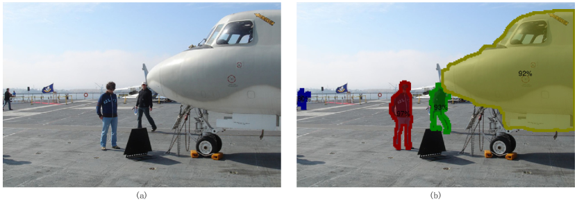
Figure 3: An example of class-independent object segmentation [8].

Class-independent object proposals: Inspired by the objectness window work of Alexi et al. [93], methods of class-independent region proposals directly attempt to produce general object regions. The underlying rationale for class-independent proposals to work is that the object-of-interest is typically distinct from background in certain appearance or geometry cues. Hence, in some sense general object proposal problem is correlated with the popular salient object detection problem. A more complete survey of state-of-the-art objectness window methods and salient object detection methods can be found in [94] and [95], respectively. Here we focus on the region proposal methods.

One group of class-independent object proposal methods is to first use bottom-up methods to generate regions proposals, and then a pre-trained classifier is applied to rank proposals according to the region features. The representative works include CPMC [8] and Category Independent Object Proposal [9], which extend GrabCut to this scenario by using different seed sampling techniques (see Fig. 3 for an example). In particular, CPMC applies sequential GrabCuts by using the regular grid as foreground seeds and image frame boundary as background seeds to train the Gaussian mixture models. Category Independent Object Proposal samples foreground seeds from occlusion boundaries inferred by [96]. Then the generated regions proposals are fed to random forests classifier or regressor, which is trained with the the features (such as convexity, color contrast, etc) of the ground truth object regions, for re-ranking. One bottleneck of such appearance based object proposal methods is that re-computing GrabCut’s appearance model implicitly incorporates the re-computation of some distance, which makes such methods hard to speed up. A recent work in [97] pre-computes a graph which can be used for parametric min-cuts over different seeds, and then dynamic graph cut [98] is applied to accelerate the speed. Instead of computing expensive GrabCut, another recent work called Geodesic Object Proposal (GOP) [99] exploits the fast geodesic distance transform for object proposals. GOP uses superpixels as its atomic units, chooses the first seed location as the one whose geodesic distance is the smallest to all other superixels, and then places next seeds far to the existing seeds. The authors also proposed to use RankSVM to learn to place seeds, but the performance improvement is not significant.

Another bottom-up way to generate region proposals is to use the edge based region merging method, gPb-OWT-UCM, described in Section 2. Then, the region hierarchies are filtered using the classifiers of CPMC. Due to its reliance on the high accuracy contour map, such method can achieve higher accuracy than GrabCut based methods. However, such method is limited by the performance of contour detectors, whose shortcomings on speed and accuracy have been greatly improved by some recently introduced learning based methods such as Structured Forest [100] or the multi-resolution eigen-solvers. The later solver has been applied in an improved version of gPb-OWT-UCM (MCG) [101] which simultaneously considers the region combinatorial space.

Different from the above class-independent object proposal methods, which use single strategy to generate object regions, another group of methods apply multiple hand-crafted strategies to produce diversified solutions during the process of atomic unit generation and region proposal generation, which we call diversified region proposal methods. This type of methods typically just produce diversified region proposals, but do not train classifier to rank the proposals. For example, SelectiveSearch [102] generates region trees from superpixels to capture objects at multiple scales by using different merging similarity metrics (such as RGB, Intensity, Texture, etc). To increase the degree of diversification, SeleciveSearch also applies different parameters to generate initial atomic superpixels. After different segmentation trees are generated, the detection starts from the regions in higher hierarchies. Manen et al. [103] proposed a similar method which exploits merging randomized trees with learned similarity metrics.

6 Semantic Image Parsing

Semantic image parsing aims to break an image into non-overlapped regions which correspond to predefined semantic classes (e.g. car, grass, sheep, etc), as shown in Fig. 4 . The popularity of semantic parsing since early 2000s is deeply rooted in the success of some specific computer vision tasks such as face/object detection and tracking, camera pose estimation, multiple view 3D reconstruction and fast conditional random field solvers. The ultimate goal of semantic parsing is to equip the computer with the holistic ability to understand the visual world around us. Although also depending on the given information, high-level learned representations make it different from the interactive methods. The learned models can be used to predict similar regions in new images. This type of approaches is also different from the object region proposal in the sense that it aims to parse an image as a whole into the “thing” and “stuff” classes, instead of just producing possible “thing” candidates.

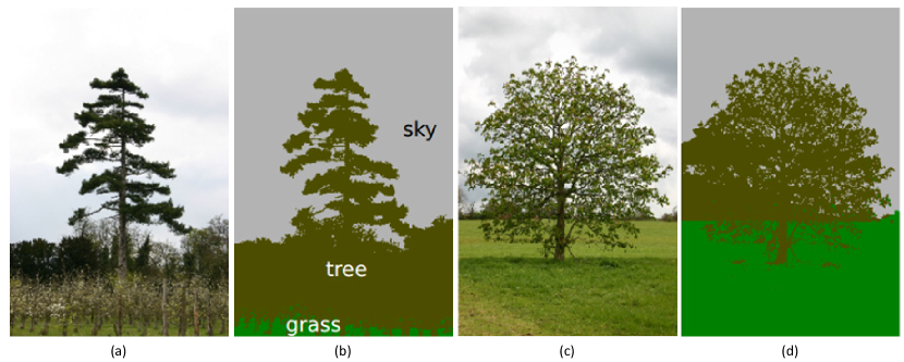
Figure 4: An example of semantic segmentation [30] which is trained using pictures with human labeled ground truth such as (b) to segment the test image in (c) and produce the final segmentation in (d).

Most state-of-the-art image parsing systems are formulated as the problem of finding the most probable labeling on a Markov random field (MRF) or conditional random field (CRF). CRF provides a principled probabilistic framework to model complex interactions between output variables and observed features. Thanks to the ability to factorize the probability distribution over different labeling of the random variables, CRF allows for compact representations and efficient inference. The CRF model defines a Gibbs distribution of the output labeling y conditioned on observed features x via an energy function $E(\textbf{y};\textbf{x})$:

$$P(\textbf{y}|\textbf{x})=\frac{1}{Z(\textbf{x})}exp\{-E(\textbf{y};\textbf{x})\},$$ (27)

where $\textbf{y}=(y_{1},y_{2},….,y_{n})$ is a vector of random variables $y_{i}$ ($n$ is the number of pixels or regions) defined on each node $i$ (pixel or superpixel), which takes a label from a predefined label set $L$ given the observed features x. $Z(\textbf{x})$ here is called partition function which ensures the distribution is properly normalized and summed to one. Computing the partition function is intractable due to the sum of exponential functions. On the other hand, such computation is not necessary given the task is to infer the most likely labeling. Maximizing a posterior of (27) is equivalent to minimize the energy function $E(\textbf{y};\textbf{x})$. A common model for pixel labeling involves a unary potential $\psi^{u}(y_{i};x)$ which is associated with each pixel, and a pairwise potential $\psi^{p}(y_{i},y_{j})$ which is associated with a pair of neighborhood pixels:

$$E(\textbf{y};\textbf{x})=\sum_{i=1}^{n}\psi^{u}(y_{i};\textbf{x})+\sum_{v_{i},v_{j}\in\cal{N}}\psi_{ij}^{p}(y_{i},y_{j};\textbf{x}).$$ (28)

Given the energy function, semantic image parsing usually follows the following pipelines: 1) Extract features from a patch centered on each pixel; 2) With the extracted features and the ground truth labels, an appearance model is trained to produce a compatible score for each training sample; 3) The trained classifier is applied on the test image’s pixel-wise features, and the output is used as the unary term; 4) The pairwise term of the CRF is defined over a 4 or 8-connected neighborhood for each pixel; 5) Perform maximum a posterior (MAP) inference on the graph. Following this common pipeline, there are different variants in different aspects:

• Features: The commonly used features are bottom-up pixel-level features such as color or texton. He et al. [104] proposed to incorporate the region and image level features. Shotton et al. [105] proposed to use spatial layout filters to represent the local information corresponding to different classes, which was later adapted to random forest framework for real-time parsing [23]. Recently, deep convolutional neural network learned features [106] have also been applied to replace the hand-crafted features, which achieves promising performance.

• Spatial support: The spatial support in step 1 can be adapted to superpixels which conform to image internal structures and make feature extraction less susceptible to noise. Also by exploiting superpixels, the complexity of the model is greatly reduces from millions of variables to only hundreds or thousands. Hoiem et al. [107] used multiple segmentations to find out the most feasible configuration. Tighe et al. [108] used superpixels to retrieve similar superpixels in the training set to generate unary term. To handle multiple superpixel hypotheses, Ladicky et al. [109] proposed the robust higher order potential, which enforces the labeling consistency between the superpixels and their underlying pixels.

• Context: The context (such as boat in the water, car on the road) has emerged as another important factor beyond the basic smoothness assumption of the CRF model. Basic context model is implicitly captured by the unary potential, e.g. the pixels with green colors are more likely to be grass class. Recently, more sophisticated class co-occurrence information has been incorporated in the model. Rabinovich et al. [110] learned label co-occurence statistic in the training set and then incorporated it into CRF as additional potential. Later the systems using multiple forms of context based on co-occurence, spatilal adjacency and appearance have been proposed in [111, 112, 108]. Ladicky et al. [31] proposed an efficient method to incorporate global context, which penalizes unlikely pairs of labels to be assigned anywhere in the image by introducing one additional variable in the GraphCut model.

• Top-down and bottom-up combination: The combination of top-down and bottom-up information has also been considered in recent scene parsing works. The bottom-up information is better at capturing stuff class which is homogeneous. On the other hand, object detectors are good at capturing thing class. Therefore, their combination helps develop a more holistic scene understanding system. There are some recent studies incorporating the sliding window detectors such as Deformable Part Model [113] or Poselet [91]. Specifically, Ladicky et al. [114] proposed the higher order robust potential based on detectors which use GrabCut to generate the shape mask to compete with bottom up cues. Floros et al. [115] instead infered the shape mask from the Implicit Shape Model top-down segmentation system [116]. Arbelaez et al. [117] used the Poselet detector to segment articulated objects. Guo and Hoiem [118] chose to use Auto-Context [119] to incorporate the detector response in their system. More recently, Tighe et al. [29] proposed to transfer the mask of training images to test images as the shape potential by using trained exemplar SVM model and achieved state-of-the-art scene parsing results.

• Inference: To optimize the energy function, various techniques can be applied, such as GraphCut, Belief-Propagation or Primal-Dual methods, etc. A complete review of recent inference methods can be found in [120]. Original CRF or MRF models are usually limited to 4-neighbor or 8-neighbor. Recently, the fully connected graphical model which connects all pixels has also become popular due to the availability of efficient approximation of the time-costly message-passing step via fast image filtering [30], with the requirement that the pairwise term should be a mixture of Gaussian kernels. Vineet et al. [121] introduced the higher order term to the fully connected CRF framework, which generalizes its application.

• Data Driven: The current pipeline needs pre-trained classifier, which is quite restrictive when new classes are included in the database. Recently some researchers have advocated for non-parametric, data-driven approach for open-universe datasets. Such approaches avoid training by retrieving similar training images from the database for segmenting the new image. Liu et al. [28] proposed to use SIFT-flow [122] to transfer masks from train images. On the other hand, Tighe et al. [108] proposed to retrieve nearest superpixel neighbor in training images and achieved comparable performance to [28].

Figure 5: (a) An example of simultaneously segmenting one common foreground object from a set of image [38]. (b) An example of multi-class cosegmentation [34].

7 Image Cosegmentation

Cosegmentation aims at extracting common objects from a set of images (see Fig. 5 for examples). It is essentially a multiple-image segmentation problem, where the very weak prior that the images contain the same objects is used for automatic object segmentation. Since it does not need any pixel level or image level object information, it is suitable for large scale image dataset segmentation and many practical applications, which attracts much attention recently. At the meanwhile, cosegmentation is challenging, which faces several major issues:

• The classical segmentation models are designed for a single image while cosegmentation deals with multiple images. How to design the cosegmentation model and minimize the model is critical for cosegmentation research.

• The common object extraction depends on the foreground similarity measurement. But the foreground usually varies, which makes the foreground similarity measurement difficult. Moreover, the model minimization is highly related to the selection of similarity measurement, which may result in extremely difficult optimization. Thus, how to measure the foreground similarities is another important issue.

• There are many practical applications with different requirements such as large-scale image cosegmentation, video cosegmentation and web image cosegmentation. Individual special needs require a cosegmentation model to be extendable to different scenarios, which is challenging.

Cosegmentation was first introduced by Rother et al. [123] in 2006. After that, many cosegmentation methods have been proposed [33, 34, 35, 36, 37, 38, 39, 40]. The existing methods can be roughly classified into three categories. The first one is to extend the existing single image based segmentation models to solve the cosegmentation problem, such as MRF cosegmentation, heat diffusion cosegmentation, RandomWalk based cosegmentation and active contour based cosegmentation. The second one is to design new cosegmentation models, such as formulating the cosegmentation as clustering problem, graph theory based proposal selection problem, metric rank based representation. The last one is to solve new emerging cosegmentation needs, such as multiple class/foreground object cosegmentation, large scale image cosegmentation and web image cosegmentation.

7.1 Cosegmentation by extending single-image segmentation models

A straight-forward way for cosegmentation is to extend classical single image based segmentation models. In general, the extended models can be represented as

$$E=E_{s}+E_{g}$$ (29)

where $E_{s}$ is the single image segmentation term, which guarantees the smoothness and the distinction between foreground and background in each image, and $E_{g}$ is the cosegmentation term, which focuses on evaluating the consistency between the foregrounds among the images. Only the segmentation of common objects can result in small values of both $E_{s}$ and $E_{g}$. Thus, the cosegmentation is formulated as minimizing the energy in (29).

Many classical segmentation models have been used to form $E_{s}$, e.g. using MRF segmentation models [123, 40] as

$$E_{s}^{MRF}=E_{u}^{MRF}+E_{p}^{MRF}$$ (30)

where $E_{u}^{MRF}$ and $E_{p}^{MRF}$ are the conventional unary potential and the pairwise potential. GraphCut algorithm is widely used to minimize the energy in (30). The cosegmentation term $E_{g}$ is used to evaluate the multiple foreground consistency, which is introduced to guarantee the common object segmentation. However, it makes the minimization of  (29) difficult. Various cosegmentation terms and their minimization methods have been carefully designed in MRF based cosegmentation models.

In particular, Rother et al. [123] evaluated the consistency by $\ell_{1}$ norm, i.e., $E_{g}=\sum_{z}(|h_{1}(z)-h_{2}(z)|)$, where $h_{1}$ and $h_{2}$ are features of the two foregrounds, and $z$ is the dimension of the feature. Adding the $\ell_{1}$ evaluation makes the minimization quite challenging. An approximation method called submodular-supermodular procedure has been proposed to minimize the model by max-flow algorithm. Mukherjee et al. [40] replaced $\ell_{1}$ with squared $\ell_{2}$ evaluation, i.e. $E_{g}=\sum_{z}(|h_{1}(z)-h_{2}(z)|)^{2}$. The $\ell_{2}$ has several advantages, such as relaxing the minimization to LP problem and using Pseudo-Boolean optimization method for minimization. But it is still an approximation solution. In order to simplify the model minimization, Hochbaum et al. [124] used reward strategy rather than penalty strategy. The rationale is that given any foreground pixel $p$ in the first image, the similar pixel $q$ in the second image will be rewarded as foreground. The global term was formulated as $E_{g}=\sum_{z}h_{1}(z)\cdot h_{2}(z)$, which is similar to the histogram based segment similarity measurement in [38], to force each foreground to be similar with the other foregrounds and also be different with their backgrounds. The energy generated with MRF model is proved to be submodular and can be efficiently solved by GraphCut algorithm. Rubio et al. [36] evaluated the foreground similarities by high order graph matching, which is introduced into MRF model to form the global term. Batra et al. [125] firstly proposed an interactive cosegmentation, where an automatic recommendation system was developed to guide the user to scribble the uncertain regions for cosegmentation refinement. Several cues such as uncertainty based cues, scribble based cues and image level cues are combined to form a recommendation map, where the regions with larger values are suggested to be labeled by the user.

Apart from MRF segmentation model, Collins et al. [126] extended RandomWalk model to solve cosegmentation, which results in a convex minimization problem with box constraints and a GPU implementation. In [127], active contour based segmentation is extended for cosegmentation, which consists of the foreground consistencies across images and the background consistencies within each image. Due to the linear similarity measurement, the minimization can be resolved by level set technique.

7.2 New cosegmentation models

The second category try to solve cosegmentation problem using new strategies rather than extending existing single segmentation models. For example, by treating the common object extraction task as a common region clustering problem, the cosegmentation problem can be solved by clustering strategy. Joulin et al. [37] treated the cosegmentation labeling as training data, and trained a supervised classifier based on the labeling to see if the given labels are able to result in maximal separation of the foreground and background classes. The cosegmentation is then formulated as searching the labels that lead to the best classification. Spectral method (Normalized Cuts) is adopted for the bottom-up clustering, and discriminative clustering is used to share the bottom-up clustering among images. The two clusterings are finally combined to form the cosegmentation model, which is solved by convex relaxation and efficient low-rank optimization. Kim et al. [128] solved cosegmentation by clustering strategy, which divides the images into hierarchical superpixel layers and describes the relationship of the superpixels using graph. Affinity matrix considering intra-image edge affinity and inter-image edge affinity is constructed. The cosegmentation can then be solved by spectral clustering strategy.

By representing the region similarity relationships as edge weights of a graph, graph theory has also been used to solve cosegmentation. In [129], by representing each image as a set of object proposals, a random forest regression based model is learned to select the object from backgrounds. The relationships between the foregrounds are formulated by fully connected graph, and the cosegmentation is achieved by loop belief propagation. Meng et al. [130] constructed directed graph structure to describe the foreground relationship by only considering the neighbouring images. The object cosegmentation is then formulated as s shortest path problem, which can be solved by dynamic programming.

Some methods try to learn the prior of common objects, which is then used to segment the common objects. Sun et al. [131] solved cosegmentation by learning discriminative part detectors of the object. By forming the positive and negative training parts from the given images and other images, the discriminative parts are learned based on the fact that the part detector of the common objects should more frequently appear in positive samples than negative samples. The problem is finally formulated as a latent SVM model learning problem with group sparsity regularization. Dai et al. [132] proposed coskech model by extending the active basis model to solve cosegmentation problem. In cosketch, a deformable shape template represented by codebook is generated to align and extract the common object. The template is introduced into unsupervised learning process to iteratively sketch the images based on the shape and segment cues and re-learn the shape and segment templates with the model parameters. By cosketch, similar shape objects can be well segmented.

There are also some other strategies. Faktor et al. [133] solved cosegmentation based on the similarity of composition, where the likelihood of the co-occurring region is high if it is non-trivial and has good match with other compositions. The co-occurring regions between images are firstly detected. Then, consensus scoring by transferring information among the regions is performed to obtain cosegments from co-occurring regions. Mukherjee et al. [39] evaluated the foreground similarity by forcing low entropy of the matrix comprised by the foreground features, which can handle the scale variation very well.

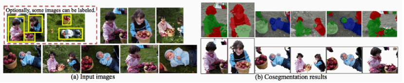
Figure 6: Given a user’s photo stream about certain event, which consists of finite objects, e.g. red-girl, blue-girl, blue-baby and apple basket. Each image contains an unknown subset of them, which we called “Multiple Foreground Cosegmentation” problem. Kim and Xing [33] proposed the first method to extract irregularly occurred objects from the photo stream (b) by using a few bounding boxes provided by the user in (a).

7.3 New cosegmentation problems

Many applications require the cosegmentation on a large-scale set of images, which is extremely time consuming. Kim et al. [34] solved the large-scale cosegmentation by temperature maximization on anisotropic heat diffusion (called CoSand), which starts with finite sources and performs heat diffusion among images based on superpixels. The model is submodular with fast solver. Wang et al. [134] proposed a semi-supervised learning based method for large scale image cosegmentation. With very limited training data, the cosegmentation is formed based on the terms of inter-image distance to measure the foreground consistencies among images, the intra-image distance to evaluate the segmentation smoothness within each image and the balance term to avoid the same label of all superpixels. The model is converted and approximated to a convex QP problem and can be solved in polynomial time using active set. Zhu et al. [135] proposed the first method which uses search engine to retrieve similar images to the input image to analyze the object-of-interest information, and then uses the information to cut-out the object-of-interest. Rubinstein et al. [136] observed that there are always noise images (which do not contain the common objects) from web image dataset, and proposed a cosegmentation model to avoid the noise images. The main idea is to match the foregrounds using SIFT flow to decide which images do not contain the common objects.

Applying cosegmentation to improve image classification is an important application of cosegmentation. Chai et al. [137] proposed a bi-level cosegmentation method, and used it for image classification. It consists of bottom level obtained by GrabCut algorithm to initialize the foregrounds and the top level with a discriminative classification to propagate the information. Later, a TriCos model [138] containing three levels were further proposed, including image level (GrabCut), dataset-level, and category level, which outperforms the bi-level model.

The sea of personal albums over internet, which depicts events in short periods, makes one popular source of large image data that need further analysis. Typical scenario of a personal album is that it contains multiple objects of different categories in the image set and each image can contain a subset of them. This is different from the classical cosegmentation models introduced above, which usually assume each image contains the same common foreground while having strong variations in backgrounds. The problem of extracting multiple objects from personal albums is called “Multiple Foreground Cosegmentation” (MFC) (see Fig. 6). Kim and Xing [33] proposed the first method to handle MFC problem. Their method starts from building apperance models (GMM & SPM) from user-provided bounding boxes which enclose the object-of-interest, and over-segments the images into superpixels by [34]. Then they used beam search to find proposal candidates for each foreground. Finally, the candidates are seamed into non-overlap regions by using dynamic programming. Ma et al. [139] formulated the multiple foreground cosegmentation as semi-supervised learning (graph transduction learning), and introduced connectivity constraints to enforce the extraction of connected regions. A cutting-plane algorithm was designed to efficiently minimize the model in polynomial time.

Kim and Ma’s methods hold an implicit constraint on objects using low-level cues, and therefore their method might assign labels of “stuff” (grass, sky) to “thing” (people or other objects). Zhu et al. [140] proposed a principled CRF framework which explicitly expresses the object constraints from object detectors and solves an even more challenging problem: multiple foreground recognition and cosegmentation (MFRC). They proposed an extended multiple color-line based object detector which can be on-line trained by using user-provided bounding boxes to detect objects in unlabeled images. Finally, all the cues from bottom-up pixels, middle-level contours and high-level object detectors are integrated in a robust high-order CRF model, which can enforce the label consistency among pixels, superpixels and object detections simultaneously, produce higher accuracy in object regions and achieve state-of-the-art performance for the MFRC problem. Later, Zhu et al. [141] further studied another challenging multiple human identification and cosegmentation problem, and proposed a novel shape cue which uses geodesic filters [83] and joint-bilateral filters to transform the blurry response maps from multiple color-line object detectors and poselet models to edge-aligned shape prior. It leads to promising human identification and co-segmentation performance.

8 Dataset and Evaluation Metrics

8.1 Datasets

To inspire new methods and objectively evaluate their performance for certain applications, different datasets and evaluation metrics have been proposed. Initially, the huge labeling cost limits the size of the datasets [142, 20] (typically in hundreds of images). Recently, with the popularity of crowdsourcing platform such as Amazon Merchant Turk (AMT) and LabelMe [143], the label cost is shared over the internet users, which makes large datasets with millions of images and labels possible. Below we summarize the most influential datasets which are widely used in the existing segmentation literature ranging from bottom-up image segmentation to holistic scene understanding:

8.1.1 Single image segmentation datasets

Berkeley segmentation benchmark dataset (BSDS) [142] is one of the earliest and largest datasets for contour detection and single image object-agnostic segmentation with human annotation. The latest BSDS dataset contains 200 images for training, 100 images for validation and the rest 200 images for testing. Each image is annotated by at least 3 subjects. Though the size of the dataset is small, it still remains one of the most difficult segmentation datasets as it contains various object classes with great pose variation, background clutter and other challenges. It has also been used to evaluate superpixel segmentation methods. Recently, Li et al. [144] proposed a new benchmark based on BSDS, which can evaluate semantic segmentation at object or part level.

MSRC-interactive segmentation dataset [20] includes 50 images with a single binary ground-truth for evaluating interactive segmentation accuracy. This dataset also provides imitated inputs such as labeling-lasso and rectangle with labels for background, foreground and unknown areas.

8.1.2 Cosegmentation datasets

MSRC-cosegmentation dataset [123] has been used to evaluate image-pair binary cosegmentation. The dataset contains 25 image pairs with similar foreground objects but heterogeneous backgrounds, which matches the assumptions of early cosegmentation methods [123, 124, 40]. Some pairs of the images are picked such that they contain some camouflage to balance database bias which forms the baseline cosegmentation dataset.

iCoseg dataset [125] is a large binary-class image cosegmentation dataset for more realistic scenarios. It contains 38 groups with a total of 643 images. The content of the images ranges from wild animals, popular landmarks, sports teams to other groups containing similar foregrounds. Each group contains images of similar object instances from different poses with some variations in the background. iCoseg is challenging because the objects are deformed considerably in terms of viewpoint and illumination, and in some cases, only a part of the object is visible. This contrasts significantly with the restrictive scenario of MSRC-Cosegmentation dataset.

FlickrMFC dataset [33] is the only dataset for multiple foreground cosegmentation, which consists of 14 groups of images with manually labeled ground-truth. Each group includes 10$\sim$20 images which are sampled from a Flikcr photostream. The image content covers daily scenarios such as children-playing, fishing, sports, etc. This dataset is perhaps the most challenging cosegmentation dataset as it contains a number of repeating subjects that are not necessarily presented in every image and there are strong occlusions, lighting variations, or scale or pose changes. Meanwhile, serious background clutters and variations often make even state-of-the-art object detectors failing on these realistic scenarios.

8.1.3 Video segmentation/cosegmentation datasets

SegTrack dataset [145] is a large binary-class video segmentation dataset with pixel-level annotation for primary objects. It contains six videos (bird, bird-fall, girl, monkey-dog, parachute and penguin). The dataset contains challenging cases including foreground/background occlusion, large shape deformation and camera motion.

CVC binary-class video cosegmentation dataset [146] contains 4 synthesis videos which paste the same foreground to different backgrounds and 2 videos sampled from the SegTrack. It forms a restrictive dataset for early video cosegmentation methods.

MPI multi-class video cosegmentation dataset [147] was proposed to evaluate video cosegmentation approaches in more challenging scenarios, which contain multi-class objects. This challenging dataset contains 4 different video sets sampled from Youtube including 11 videos with around 520 frames with ground truth. Each video set has different numbers of object classes appearing in them. Moreover, the dataset includes challenging lighting, motion blur and image condition variations.

Cambridge-driving video dataset (CamVid) [148] is a collection of videos with labels of 32 semantic classes (e.g. building, tree, sidewalk, traffic light, etc), which are captured by a position-fixed CCTV-camera on a driving automobile over 10 mins at 30Hz footage. This dataset contains 4 video sequences, with more than 700 images at resolution of $960\times 720$. Three of them are sampled at the day light condition and the remaining one is sampled at the dark. The number and the heterogeneity of the object classes in each video sequence are diverse.

8.1.4 Static scene parsing datasets

MSRC 23-class dataset [23] consists of 23 classes and 591 images. Due to the rarity of ‘horse’ and ‘mountain’ classes, these two classes are often ignored for training and evaluation. The remaining 21 classes contain diverse objects. The annotated ground-truth is quite rough.

PASCAL VOC dataset [149] provides a large-scale dataset for evaluating object detection and semantic segmentation. Starting from the initial 4-class objects in 2005, now PASCAL dataset includes 20 classes of objects under four major categories (animal, person, vehicle and indoor). The latest train/val dataset has 11,530 images and 6,929 segmentations.

LabelMe + SUN dataset: LabelMe [143] is initiated by the MIT CSCAIL which provides a dataset of annotated images. The dataset is still growing. It contains copyright-free images and is open to public contribution. As of October 31, 2010, LabelMe has 187,240 images, 62,197 annotated images, and 658,992 labeled objects. SUN [150] is a subsampled dataset from LabelMe. It contains 45,676 image (21,182 indoor and 24,494 outdoor), total 515 object categories. One noteworthy point is that the number of objects in each class is uneven, which can cause unsatisfactory segmentation accuracy for rare classes.

SIFT-flow dataset: The popularity of nonparametric scene parsing requires a large labeled dataset. The SIFT Flow dataset [122] is composed of 2,688 images that have been thoroughly labelled by LabelMe users. Liu et al. [122] have split this dataset into 2,488 training images and 200 test images and used synonym correction to obtain 33 semantic labels.

Stanford background dataset [27] consists of around 720 images sampled from the existing datasets such as LabelMe, MSRC and PASCAL VOC, whose content consists of rural, urban and harbor scenes. Each image pixel is given two labels: one for its semantic class (sky, tree, road, grass, water, building, mountain and foreground) and the one for geometric property (sky, vertical, and horizontal).

NYU dataset [151]: The NYU-depth V2 dataset is comprised of video sequences from a variety of indoor scenes recorded by both the RGB and depth cameras of Microsoft Kinect. It features 1449 densely labeled pairs of aligned RGB and depth images, 464 new scenes taken from 3 cities, and 407,024 new unlabeled frames. Each object is labeled with a class and an instance number (cup1, cup2, cup3, etc).

Microsoft COCO [152] is a recent dataset for holistic scene understanding, which provides 328K images with 91 object classes. One substantial difference with other large datasets, such as PASCAL VOC and SUN datasets, is that Microsoft COCO contains more labelled instances in million units. The authors argue that it can facilitate training object detectors with better localization, and learning contextual information.

8.2 Evaluation metrics

As segmentation is an ill-defined problem, how to evaluate an algorithm’s goodness remains an open question. In the past, the evaluation were mainly conducted through subjective human inspections or by evaluating the performance of subsequent vision system which uses image segmentation. To objectively evaluate a method, it is desirable to associate the segmentation with perceptual grouping. Current trend is to develop a benchmark [142] which consists of human-labeled segmentation and then compares the algorithm’s output with the human-labeled results using some metrics to measure the segmentation quality. Various evaluation metrics have been proposed:

• Boundary Matching: This method works by matching the algorithm-generated boundaries with human-labeled boundaries, and then computing some metric to evaluate the matching quality. Precision and recall framework proposed by Martin et al. [153] is among the widely used evaluation metrics, where the Precision measures the proportion of how many machine-generated boundaries can be found in human-labeled boundaries and is sensitive to over-segmentation, while the Recall measures the proportion of how many human-labelled boundaries can be found in machine-generated boundaries and is sensitive to under-segmentation. In general, this method is sensitive to the granularity of human labeling.

• Region Covering : This method [153] operates by checking the overlap between the machine-generated regions and human-labelled regions. Let $S_{seg}$ and $S_{hum}$ denote the machine segmentation and the human segmentation, respectively. Denote the corresponding segment regions for pixel $p_{i}$ from the pixel set $P=\{p_{1},p_{2},...,p_{n}\}$ as $C(S_{seg},p_{i})$ and $C(S_{hum},p_{i})$. The relative region covering error at $p_{i}$ is

  $$O(S_{seg},S_{label},p_{i})=\frac{|C(S_{seg},p_{i})\setminus C(S_{hum},p_{i})|}{C(S_{seg},p_{i})}.$$ (31)

  where $\setminus$ is the set differencing operator.

  The globe region covering error is defined as:

  $$\begin{split}&GCE(S_{seg},S_{label})=\\ &\frac{1}{n}min\{\sum_{i}O(S_{seg},S_{label},p_{i}),O(S_{label},S_{seg},p_{i})\}.\end{split}$$ (32)

  However, when each pixel is a segment or the whole image is a segment, the $GCE$ becomes zero which is undesirable. To alleviate these problems, the authors proposed to replace $min$ operation by using $max$ operation, but such change will not encourage segmentation at finer detail.

  Another commonly used region based criterion is the Intersection-over-Union, by checking the overlap between the $S_{seg}$ and $S_{hum}$:

  $$IoU(S_{seg},S_{hum})=\frac{S_{Seg}\cap S_{hum}}{S_{Seg}\cup S_{hum}}$$ (33)

• Variation of Information (VI): This metric [154] measures the distance between two segmentations $S_{seg}$ and $S_{hum}$ using average conditional entropy. Assume that $S_{seg}$ and $S_{hum}$ have clusters $C_{seg}=\{C_{seg}^{1},C_{seg}^{2},...,C_{seg}^{K}\}$ and $C_{hum}=\{C_{hum}^{1},C_{hum}^{2},...,C_{hum}^{K^{\prime}}\}$, respectively. The variation of information is defined as:

  $$VI(S_{seg},S_{hum})=H(S_{seg})+H(S_{hum})-2I(S_{seg},S_{hum})$$ (34)

  where $H(S_{seg})$ is the entropy associated with clustering $S_{seg}$:

  $$H(S_{seg})=-\sum_{k=1}^{K}P(k)logP(k)$$ (35)

  with $P(k)=\frac{n_{k}}{n}$, where $n_{k}$ is the number of elements in cluster $k$ and $n$ is the total number of elements in $S_{seg}$. $I(S_{seg},S_{hum})$ is the mutual information between $S_{seg}$ and $S_{hum}$:

  $$I(S_{seg},S_{hum})=\sum_{k=1}^{K}\sum_{k^{\prime}=1}^{K^{\prime}}P(k,k^{\prime})log\frac{P(k,k^{\prime})}{P(k)P(k^{\prime})}$$ (36)

  with $P(k,k^{\prime})=\frac{|C_{seg}^{k}\bigcap C_{hum}^{k}|}{n}$.

  Although $VI$ posses some interesting property, its perceptual meaning and potential in evaluating more than one ground-truth are unknown [48].

• Probabilistic Random Index (PRI): PRI was introduced to measure the compatibility of assignments between pairs of elements in $S_{seg}$ and $S_{hum}$. It has been defined to deal with multiple ground-truth segmentations [155]:

  $$PRI(S_{seg},S_{hum}^{k})=\frac{1}{\frac{N}{2}}\sum_{i<j}[c_{ij}p_{ij}+(1-c_{ij})(1-p_{ij})]$$ (37)

  where $S_{hum}^{k}$ is the $k$-th human-labeled ground-truth, $c_{ij}$ is the event that pixels $i$ and $j$ have the same label and $p_{ij}$ is the corresponding probability. As reported in [50], the PRI has a small dynamic range and the values across images and algorithms are often similar which makes the differentiation difficult.

9 Discussions and Future Directions

9.1 Design flavors

When designing a new segmentation algorithm, it is often difficult to make choices among various design flavors, e.g. to use superpixel or not, to use more images or not. It all depends on the applications. Our literature review has cast some lights on the pros and cons of some commonly used design flavors, which is worth thinking twice before going ahead for a specific setup.

Patch vs. region vs. object proposal: Careful readers might notice that there has been a significant trend in migrating from patch based analysis to region based (or superpixel based) analysis. The continuous performance improvement in terms of boundary recall and execution time makes superpixel a fast preprocessing technique. The advantages of using superpixel lie in not only the time reduction in training and inference but also more complex and discriminative features that can be exploited. On the other hand, superpixel itself is not perfect, which could introduce new structure errors. For users who care more about visual results on the segment boundary, pixel-based or hybrid approach of combining pixel and superpixel should be considered as better options. The structure errors of using superpixel can also be alleviated by using different methods and parameters to produce multiple over-segmentation or using fast edge-aware filtering to refine the boundary. For users more caring about localization accuracy, the region based way is more preferred due to the various advantages introduced while the boundary loss can be neglected. Another uprising trend that is worth mentioning is the application of the object region proposals [129, 130]. Due to the larger support provided by object-like regions than oversegmentation or pixels, more complex classifiers and region-level features can be extracted. However, the recall rate of the object proposal is still not satisfactory (around $60\%$); therefore more careful designs need to be made when accuracy is a major concern.

Intrinsic cues vs. extrinsic cues: Although intrinsic cues (the features and prior knowledge for a single image) still play dominant roles in existing CV applications, extrinsic cues which come from multiple images (such as multiview images, video sequence, and a super large image dataset of similar products) are attracting more and more attentions. An intuitive answer why extrinsic cues convey more semantics can be interpreted in terms of statistic. When there are many signals available, the signals which repeatedly appear form patterns of interest, while those errors are averaged. Therefore, if there are multiple images containing redundant but diverse information, incorporating extrinsic cues should bring some improvements. When taking extrinsic cues, the source of information needs to be considered in the algorithm design. More robust constraints such as the cues from multiple-view geometric or spatial-temporal relationships should be exploited first. When working with external information such as a large dataset which contains heterogeneous data, a mechanism that can handle noisy information should be developed.

Hand-crafted features vs. learned features: Hand-crafted features, such as intensity, color, SIFT and Bag-of-Word, etc, have played important roles in computer vision. These simple and training-free features have been applied to many applications, and their effectiveness has been widely examined. However, the generalization capability of these hand-crafted features from one task to another task depends on the heuristic feature design and combination, which can compromise the performance. The development of low-level features has become more and more challenging. On the other hand, learned features from labelled database have recently been demonstrated advantages in some applications, such as scene understanding and object detection. The effectiveness of the learned features comes from the context information captured from longer spatial arrangement and higher order co-occurrence. With labelled data, some structured noise is eliminated which helps highlight the salient structures. However, learned features can only detect patterns for certain tasks. If migrating to other tasks, it needs newly labelled data, which is time consuming and expensive to obtain. Therefore, it is suggested to choose features from the handcraft features first. If it happens to have labelled data, then using learned features usually boost up the performance.

9.2 Promising future directions

Based on the discussed literature and the recent development in segmentation community, here we suggest some future directions which is worth for exploring:

Beyond single image: Although single image segmentation has played a dominant role in the past decades, the recent trend is to use the internal structures of multiple images to facilitate segmentation. When human perceives a scene, the motion cues and depth cues provide extra information, which should not be neglected. For example, when the image data is from a video, the 3D geometry estimated from the structure-from-motion techniques can be used to help image understanding [156, 157]. The depth information captured by commodity depth cameras such as Kinect also benefits the indoor scene understanding [158, 159]. Beyond 3D information, the useful information from other 2D images in a large database, either organized (like ImageNet) or un-organized (like product or animal category), or multiple heterogeneous datasets of the same category, can also be exploited [160, 161].

Toward multiple instances: Most segmentation methods still aim to produce a most likely solution, e.g. all pixels of the same category are assigned the same label. On the other hand, people are also interested in knowing the information of “how many” of the same category objects are there, which is a limitation of the existing works. Recently, there are some works making efforts towards this direction by combining state-of-the-art detectors with the CRF modelling [114, 162, 163] which have achieved some progress. In addition, the recently developed dataset, Microsoft COCO [152], which contains many images with labelled instances, can be expected to boost the development in this direction.

Become more holistic: Most existing works consider the image labelling task alone [104, 23]. On the other hand, studying a related task can improve the existing scene analysis problem. For example, by combining the object detection with image classification, Yao et al. [164] proposed a more robust and accurate system than the ones which perform single task analysis. Such holistic understanding trend can also be seen from other works, by combining context [110, 165], geometry [27, 166, 107, 167], attributes [168, 169, 170, 171, 172] or even language [173, 174]. It is therefore expected that a more holistic system should lead to better performance than those performing monotone analysis, though at an increasing inference cost.

Go from shallow to deep: Feature has been played an important role in many vision applications, e.g. stereo matching, detection and segmentation. Good features, which are highly discriminative to differentiate ‘object’ from ‘stuff’, can help object segmentation significantly. However, most features today are hand-crafted designed for specific tasks. When applied to other tasks, the hand-crafted features might not generalize well. Recently, learned features using multiple-layer neural network [175] have been applied in many vision tasks, including object classification [176], face detection [177], pose estimation [178], object detection [179] and semantic segmentation [106], and achieved state-of-the-art performance. Therefore, it is interesting to explore whether such learned features can benefit the aforementioned more complex tasks.

10 Conclusion

In this paper, we have conducted a thorough review of recent development of image segmentation methods, including classic bottom-up methods, interactive methods, object region proposals, semantic parsing and image cosegmentation. We have discussed the pros and cons of different methods, and suggested some design choices and future directions which are worthwhile for exploration.

Segmentation as a community has achieved substantial progress in the past decades. Although some technologies such as interactive segmentation have been commercialized in recent Adobe and Microsoft products, there is still a long way to make segmentation a general and reliable tool to be widely applied to practical applications. This is more related to the existing methods’ limitations in terms of robustness and efficiency. For example, one can always observe that given images under various degradations (strong illumination change, noise corruption or rain situation), the performance of the existing methods could drop significantly [180]. With the rapid improvement in computing hardware, more effective and robust methods will be developed, where the breakthrough is likely to come from the collaborations with other engineering and science communities, such as physics, neurology and mathematics.

References

- [1] C. Carson, S. Belongie, H. Greenspan, J. Malik, Blobworld: Image segmentation using expectation-maximization and its application to image querying, IEEE Trans. Pattern Anal. Mach. Intell. 24 (8) (2002) 1026–1038.
- [2] R. Achanta, A. Shaji, K. Smith, A. Lucchi, P. Fua, S. Süsstrunk, Slic superpixels compared to state-of-the-art superpixel methods, IEEE Trans. Pattern Anal. Mach. Intell. 34 (11).
- [3] D. Comaniciu, P. Meer, Mean shift: A robust approach toward feature space analysis, IEEE Trans. Pattern Anal. Mach. Intell. 24 (5) (2002) 603–619.
- [4] J. Lu, H. Yang, D. Min, M. N. Do, Patch match filter: Efficient edge-aware filtering meets randomized search for fast correspondence field estimation, in: CVPR, 2013.
- [5] P. Kohli, M. P. Kumar, P. H. S. Torr, P & beyond: Move making algorithms for solving higher order functions, IEEE Trans. Pattern Anal. Mach. Intell. 31 (9).
- [6] G. Mori, Guiding model search using segmentation, in: ICCV, 2005.
- [7] C. Gu, J. J. Lim, P. Arbelaez, J. Malik, Recognition using regions, in: CVPR, 2009.
- [8] J. Carreira, C. Sminchisescu, Cpmc: Automatic object segmentation using constrained parametric min-cuts, IEEE Trans. Pattern Anal. Mach. Intell. 34 (7).
- [9] I. Endres, D. Hoiem, Category-independent object proposals with diverse ranking, IEEE Trans. Pattern Anal. Mach. Intell. 36 (2).
- [10] J. Shi, J. Malik, Normalized cuts and image segmentation, IEEE Trans. Pattern Anal. Mach. Intell. 22 (8) (2000) 888–905.
- [11] D. R. Martin, C. Fowlkes, J. Malik, Learning to detect natural image boundaries using local brightness, color, and texture cues, IEEE Trans. Pattern Anal. Mach. Intell.
- [12] D. D. Hoffman, M. Singh, Salience of visual parts, Cognition 63 (1) (1997) 29 – 78. doi:10.1016/S0010-0277(96)00791-3.
- [13] R. Ohlander, K. Price, D. R. Reddy, Picture segmentation using a recursive region splitting method, Computer Graphics and Image Processing 8 (1978) 313–333.
- [14] C. R. Brice, C. L. Fennema, Scene analysis using regions., Artif. Intell. 1 (3) (1970) 205–226.
- [15] P. F. Felzenszwalb, D. P. Huttenlocher, Efficient graph-based image segmentation, International Journal of Computer Vision 59 (2) (2004) 167–181.
- [16] L. Vincent, P. Soille, Watersheds in digital spaces: An efficient algorithm based on immersion simulations, IEEE Trans. Pattern Anal. Mach. Intell. 13 (6) (1991) 583–598.
- [17] R. Beare, A locally constrained watershed transform, IEEE Trans. Pattern Anal. Mach. Intell. 28 (7) (2006) 1063–1074.
- [18] T. F. Chan, L. A. Vese, Active contours without edges, IEEE Transactions on Image Processing 10 (2) (2001) 266–277.
- [19] S. Osher, J. A. Sethian, Fronts propagating with curvature dependent speed: Algorithms based on hamilton-jacobi formulations, Journal of Computational Physics 79 (1) (1988) 12–49.
- [20] C. Rother, V. Kolmogorov, A. Blake, Grabcut: interactive foreground extraction using iterated graph cuts, ACM Trans. Graph. 23 (3).
- [21] W. Yang, J. Cai, J. Zheng, J. Luo, User-friendly interactive image segmentation through unified combinatorial user inputs, IEEE Transactions on Image Processing 19 (9) (2010) 2470–2479.
- [22] T. N. A. Nguyen, J. Cai, J. Zhang, J. Zheng, Robust interactive image segmentation using convex active contours, IEEE Transactions on Image Processing 21 (8) (2012) 3734–3743.
- [23] J. Shotton, J. M. Winn, C. Rother, A. Criminisi, Textonboost for image understanding: Multi-class object recognition and segmentation by jointly modeling texture, layout, and context, International Journal of Computer Vision 81 (1).
- [24] P. F. Felzenszwalb, R. B. Girshick, D. A. McAllester, Cascade object detection with deformable part models, in: CVPR, 2010.
- [25] D. Hoiem, A. A. Efros, M. Hebert, Putting objects in perspective., International Journal of Computer Vision 80 (1) (2008) 3–15.
- [26] P. Kohli, L. Ladicky, P. H. S. Torr, Robust higher order potentials for enforcing label consistency, International Journal of Computer Vision 82 (3).
- [27] S. Gould, R. Fulton, D. Koller, Decomposing a scene into geometric and semantically consistent regions, in: ICCV, 2009.
- [28] C. Liu, J. Yuen, A. Torralba, Nonparametric scene parsing via label transfer, IEEE Trans. Pattern Anal. Mach. Intell. 33 (12).
- [29] J. Tighe, S. Lazebnik, Finding things: Image parsing with regions and per-exemplar detectors, in: CVPR, 2013.
- [30] P. Krähenbühl, V. Koltun, Efficient inference in fully connected crfs with gaussian edge potentials, in: NIPS, 2011, pp. 109–117.
- [31] L. Ladicky, C. Russell, P. Kohli, P. H. S. Torr, Graph cut based inference with co-occurrence statistics, in: ECCV, 2010.
- [32] J. Deng, W. Dong, R. Socher, L.-J. Li, K. Li, F.-F. Li, Imagenet: A large-scale hierarchical image database, in: CVPR, 2009.
- [33] G. Kim, E. P. Xing, On multiple foreground cosegmentation, in: CVPR, 2012, pp. 837–844.
- [34] G. Kim, E. P. Xing, F.-F. Li, T. Kanade, Distributed cosegmentation via submodular optimization on anisotropic diffusion, in: ICCV, 2011, pp. 169–176.
- [35] A. Joulin, F. Bach, J. Ponce, Multi-class cosegmentation, in: CVPR, 2012.
- [36] J. C. Rubio, J. Serrat, A. M. López, N. Paragios, Unsupervised co-segmentation through region matching, in: CVPR, 2012.
- [37] A. Joulin, F. R. Bach, J. Ponce, Discriminative clustering for image co-segmentation, in: CVPR, 2010, pp. 1943–1950.
- [38] K.-Y. Chang, T.-L. Liu, S.-H. Lai, From co-saliency to co-segmentation: An efficient and fully unsupervised energy minimization model, in: CVPR, 2011, pp. 2129–2136.
- [39] L. Mukherjee, V. Singh, J. Peng, Scale invariant cosegmentation for image groups, in: CVPR, 2011.
- [40] L. Mukherjee, V. Singh, C. R. Dyer, Half-integrality based algorithms for cosegmentation of images, in: CVPR, 2009.
- [41] R. Szeliski, Computer Vision - Algorithms and Applications, Texts in Computer Science, Springer, 2011.
- [42] S. Rao, H. Mobahi, A. Y. Yang, S. Sastry, Y. Ma, Natural image segmentation with adaptive texture and boundary encoding, in: ACCV, 2009.
- [43] J. Shi, J. Malik, Normalized cuts and image segmentation, in: CVPR, 1997.
- [44] J. Malik, S. Belongie, J. Shi, T. K. Leung, Textons, contours and regions: Cue integration in image segmentation, in: ICCV, 1999.
- [45] B. Cheng, G. Liu, J. Wang, Z. Huang, S. Yan, Multi-task low-rank affinity pursuit for image segmentation, in: ICCV, 2011.
- [46] A. Y. Ng, M. I. Jordan, Y. Weiss, On spectral clustering: Analysis and an algorithm, in: NIPS, 2001, pp. 849–856.
- [47] T. Cour, F. Bénézit, J. Shi, Spectral segmentation with multiscale graph decomposition, in: CVPR, 2005, pp. 1124–1131.
- [48] P. Arbelaez, M. Maire, C. C. Fowlkes, J. Malik, From contours to regions: An empirical evaluation, in: CVPR, 2009.
- [49] A. K. Jain, A. P. Topchy, M. H. C. Law, J. M. Buhmann, Landscape of clustering algorithms, in: ICPR (1), 2004, pp. 260–263.
- [50] P. Arbelaez, M. Maire, C. Fowlkes, J. Malik, Contour detection and hierarchical image segmentation, IEEE Trans. Pattern Anal. Mach. Intell. 33 (5) (2011) 898–916.
- [51] X. Bresson, S. Esedoglu, P. Vandergheynst, J.-P. Thiran, S. Osher, Fast global minimization of the active contour/snake model, Journal of Mathematical Imaging and Vision 28 (2) (2007) 151–167.
- [52] T. Pock, A. Chambolle, D. Cremers, H. Bischof, A convex relaxation approach for computing minimal partitions, in: CVPR, 2009, pp. 810–817.
- [53] J. Yuan, E. Bae, X.-C. Tai, Y. Boykov, A continuous max-flow approach to potts model, in: ECCV, 2010, pp. 379–392.
- [54] L. Ambrosio, V. Tortorelli, Approximation of functionals depending on jumps by elliptic functionals via -convergence, Communications on Pure and Applied Mathematics XLIII (1990) 999–1036.
- [55] A. Braides, G. Dal Maso, Non-local approximation of the mumford-shah functional, Calculus of Variations and Partial Differential Equations 5 (4) (1997) 293–322. doi:10.1007/s005260050068.
- [56] A. Braides, Approximation of Free-Discontinuity Problems, Vol. 1694 of Lecture Notes in Mathematics, Springer, 1998.
- [57] A. Chambolle, Image segmentation by variational methods: Mumford and shah functional and the discrete approximations, SIAM J. Appl. Math. 55 (3) (1995) 827–863. doi:10.1137/S0036139993257132.
- [58] L. A. Vese, T. F. Chan, A multiphase level set framework for image segmentation using the mumford and shah model, International Journal of Computer Vision 50 (3) (2002) 271–293.
- [59] M. Kass, A. Witkin, D. Terzopoulos, Snakes: Active contour models, International Journal of Computer Vision 1 (4) (1988) 321–331. doi:10.1007/BF00133570.
- [60] H. Zhu, J. Zheng, J. Cai, N. Magnenat-Thalmann, Object-level image segmentation using low level cues, IEEE Transactions on Image Processing 22 (10) (2013) 4019–4027.
- [61] X. Ren, J. Malik, Learning a classification model for segmentation, in: ICCV, 2003, pp. 10–17.
- [62] A. Levinshtein, A. Stere, K. N. Kutulakos, D. J. Fleet, S. J. Dickinson, K. Siddiqi, Turbopixels: Fast superpixels using geometric flows, IEEE Trans. Pattern Anal. Mach. Intell. 31 (12) (2009) 2290–2297.
- [63] P. Wang, G. Zeng, R. Gan, J. Wang, H. Zha, Structure-sensitive superpixels via geodesic distance, International Journal of Computer Vision 103 (1) (2013) 1–21.
- [64] O. Veksler, Y. Boykov, P. Mehrani, Superpixels and supervoxels in an energy optimization framework, in: Computer Vision - ECCV 2010 - 11th European Conference on Computer Vision, Heraklion, Crete, Greece, September 5-11, 2010, Proceedings, Part V, 2010, pp. 211–224.
- [65] Y. Zhang, R. I. Hartley, J. Mashford, S. Burn, Superpixels via pseudo-boolean optimization, in: ICCV, 2011, pp. 1387–1394.
- [66] M. Liu, O. Tuzel, S. Ramalingam, R. Chellappa, Entropy-rate clustering: Cluster analysis via maximizing a submodular function subject to a matroid constraint, IEEE Trans. Pattern Anal. Mach. Intell. 36 (1) (2014) 99–112.
- [67] M. V. den Bergh, X. Boix, G. Roig, B. de Capitani, L. J. V. Gool, SEEDS: superpixels extracted via energy-driven sampling, in: ECCV, 2012, pp. 13–26.
- [68] K. McGuinness, N. E. O’Connor, A comparative evaluation of interactive segmentation algorithms, Pattern Recognition 43 (2) (2010) 434–444.
- [69] F. Yi, I. Moon, Image segmentation: A survey of graph-cut methods, in: Systems and Informatics (ICSAI), 2012 International Conference on, 2012.
- [70] J. He, C.-S. Kim, C.-C. J. Kuo, Interactive Segmentation Techniques: Algorithms and Performance Evaluation, Springer Publishing Company, Incorporated, 2013.
- [71] M. Kass, A. P. Witkin, D. Terzopoulos, Snakes: Active contour models, International Journal of Computer Vision 1 (4) (1988) 321–331.
- [72] E. Mortensen, B. Morse, W. Barrett, J. Udupa, Adaptive boundary detection using ‘live-wire’ two-dimensional dynamic programming, in: Computers in Cardiology 1992, Proceedings of, 1992, pp. 635–638.
- [73] Y. Boykov, M.-P. Jolly, Interactive graph cuts for optimal boundary and region segmentation of objects in n-d images, in: ICCV, 2001, pp. 105–112.
- [74] E. N. Mortensen, W. A. Barrett, Intelligent scissors for image composition, in: SIGGRAPH, 1995, pp. 191–198.
- [75] Y. Liu, Y. Yu, Interactive image segmentation based on level sets of probabilities, IEEE Trans. Vis. Comput. Graph. 18 (2) (2012) 202–213.
- [76] L. Grady, Random walks for image segmentation, IEEE Trans. Pattern Anal. Mach. Intell. 28 (11) (2006) 1768–1783.
- [77] Y. Li, J. Sun, C. Tang, H. Shum, Lazy snapping, ACM Trans. Graph. 23 (3) (2004) 303–308.
- [78] P. Kohli, A. Osokin, S. Jegelka, A principled deep random field model for image segmentation, in: CVPR, 2013, pp. 1971–1978.
- [79] B. L. Price, B. S. Morse, S. Cohen, Geodesic graph cut for interactive image segmentation, in: CVPR, 2010, pp. 3161–3168.
- [80] X. Bai, G. Sapiro, A geodesic framework for fast interactive image and video segmentation and matting, in: ICCV, 2007, pp. 1–8.
- [81] O. Veksler, Star shape prior for graph-cut image segmentation, in: Computer Vision - ECCV 2008, 10th European Conference on Computer Vision, Marseille, France, October 12-18, 2008, Proceedings, Part III, 2008, pp. 454–467.
- [82] V. Gulshan, C. Rother, A. Criminisi, A. Blake, A. Zisserman, Geodesic star convexity for interactive image segmentation, in: The Twenty-Third IEEE Conference on Computer Vision and Pattern Recognition, CVPR 2010, San Francisco, CA, USA, 13-18 June 2010, 2010, pp. 3129–3136.
- [83] A. Criminisi, T. Sharp, A. Blake, Geos: Geodesic image segmentation, in: Computer Vision - ECCV 2008, 10th European Conference on Computer Vision, Marseille, France, October 12-18, 2008, Proceedings, Part I, 2008, pp. 99–112.
- [84] S. Vicente, V. Kolmogorov, C. Rother, Graph cut based image segmentation with connectivity priors, in: CVPR, 2008.
- [85] A. Hosni, C. Rhemann, M. Bleyer, C. Rother, M. Gelautz, Fast cost-volume filtering for visual correspondence and beyond, IEEE Trans. Pattern Anal. Mach. Intell. 35 (2) (2013) 504–511.
- [86] F. Durand, J. Dorsey, Fast bilateral filtering for the display of high-dynamic-range images, ACM Trans. Graph. 21 (3) (2002) 257–266.
- [87] K. He, J. Sun, X. Tang, Guided image filtering, IEEE Trans. Pattern Anal. Mach. Intell. 35 (6) (2013) 1397–1409.
- [88] J. Lu, K. Shi, D. Min, L. Lin, M. N. Do, Cross-based local multipoint filtering, in: CVPR, 2012, pp. 430–437.
- [89] R. Adams, L. Bischof, Seeded region growing, IEEE Trans. Pattern Anal. Mach. Intell. 16 (6) (1994) 641–647.
- [90] J. Ning, L. Zhang, D. Zhang, C. Wu, Interactive image segmentation by maximal similarity based region merging, Pattern Recognition 43 (2) (2010) 445–456.
- [91] L. D. Bourdev, S. Maji, T. Brox, J. Malik, Detecting people using mutually consistent poselet activations, in: ECCV, 2010.
- [92] D. Larlus, F. Jurie, Combining appearance models and markov random fields for category level object segmentation, in: CVPR, 2008.
- [93] B. Alexe, T. Deselaers, V. Ferrari, Measuring the objectness of image windows, IEEE Trans. Pattern Anal. Mach. Intell. 34 (11) (2012) 2189–2202.
- [94] J. Hosang, R. Benenson, B. Schiele, How good are detection proposals, really?, in: British Machine Vision Conference (BMVC), British Machine Vision Association, British Machine Vision Association, 2014.
- [95] A. Borji, M. Cheng, H. Jiang, J. Li, Salient object detection: A survey, CoRR abs/1411.5878.
- [96] D. Hoiem, A. A. Efros, M. Hebert, Recovering occlusion boundaries from an image, International Journal of Computer Vision 91 (3) (2011) 328–346.
- [97] A. Humayun, F. Li, J. M. Rehg, RIGOR: reusing inference in graph cuts for generating object regions, in: CVPR, 2014, pp. 336–343.
- [98] P. Kohli, J. Rihan, M. Bray, P. H. S. Torr, Simultaneous segmentation and pose estimation of humans using dynamic graph cuts, International Journal of Computer Vision 79 (3) (2008) 285–298.
- [99] P. Krähenbühl, V. Koltun, Geodesic object proposals, in: Computer Vision - ECCV 2014 - 13th European Conference, Zurich, Switzerland, September 6-12, 2014, Proceedings, Part V, 2014, pp. 725–739.
- [100] P. Dollár, C. L. Zitnick, Structured forests for fast edge detection, in: ICCV, 2013, pp. 1841–1848.
- [101] P. A. Arbeláez, J. Pont-Tuset, J. T. Barron, F. Marqués, J. Malik, Multiscale combinatorial grouping, in: CVPR, 2014, pp. 328–335.
- [102] K. E. A. van de Sande, J. R. R. Uijlings, T. Gevers, A. W. M. Smeulders, Segmentation as selective search for object recognition, in: ICCV, 2011, pp. 1879–1886.
- [103] S. Manen, M. Guillaumin, L. J. V. Gool, Prime object proposals with randomized prim’s algorithm., in: ICCV, 2013.
- [104] X. He, R. S. Zemel, M. . Carreira-Perpiñán, Multiscale conditional random fields for image labeling., in: CVPR, 2004, pp. 695–702.
- [105] J. Shotton, M. Johnson, R. Cipolla, Semantic texton forests for image categorization and segmentation., in: CVPR, 2008.
- [106] C. Farabet, C. Couprie, L. Najman, Y. LeCun, Learning hierarchical features for scene labeling, IEEE Trans. Pattern Anal. Mach. Intell. 35 (8) (2013) 1915–1929. doi:10.1109/TPAMI.2012.231.
- [107] D. Hoiem, A. A. Efros, M. Hebert, Recovering surface layout from an image, International Journal of Computer Vision 75 (1) (2007) 151–172.
- [108] J. Tighe, S. Lazebnik, Superparsing - scalable nonparametric image parsing with superpixels., International Journal of Computer Vision 101 (2) (2013) 329–349.
- [109] L. Ladicky, C. Russell, P. Kohli, P. H. S. Torr, Associative hierarchical crfs for object class image segmentation, in: IEEE 12th International Conference on Computer Vision, ICCV 2009, Kyoto, Japan, September 27 - October 4, 2009, 2009, pp. 739–746.
- [110] A. Rabinovich, A. Vedaldi, C. Galleguillos, E. Wiewiora, S. Belongie, Objects in context., in: ICCV, 2007, pp. 1–8.
- [111] C. Galleguillos, A. Rabinovich, S. Belongie, Object categorization using co-occurrence, location and appearance., in: CVPR, 2008.
- [112] C. Galleguillos, B. McFee, S. J. Belongie, G. R. G. Lanckriet, Multi-class object localization by combining local contextual interactions., in: CVPR, IEEE, 2010, pp. 113–120.
- [113] P. F. Felzenszwalb, D. A. McAllester, D. Ramanan, A discriminatively trained, multiscale, deformable part model., in: CVPR, 2008.
- [114] L. Ladicky, P. Sturgess, K. Alahari, C. Russell, P. H. S. Torr, What, where and how many? combining object detectors and crfs, in: ECCV, 2010.
- [115] G. Floros, K. Rematas, B. Leibe, Multi-class image labeling with top-down segmentation and generalized robust $p^n$ potentials, in: British Machine Vision Conference, BMVC 2011, Dundee, UK, August 29 - September 2, 2011. Proceedings, 2011.
- [116] B. Leibe, A. Leonardis, B. Schiele, Robust object detection with interleaved categorization and segmentation., International Journal of Computer Vision 77 (1-3) (2008) 259–289.
- [117] P. Arbelaez, B. Hariharan, C. Gu, S. Gupta, L. D. Bourdev, J. Malik, Semantic segmentation using regions and parts, in: CVPR, 2012, pp. 3378–3385.
- [118] R. Guo, D. Hoiem, Beyond the line of sight: Labeling the underlying surfaces., in: A. W. Fitzgibbon, S. Lazebnik, P. Perona, Y. Sato, C. Schmid (Eds.), ECCV, Lecture Notes in Computer Science, Springer, 2012, pp. 761–774.
- [119] Z. Tu, Auto-context and its application to high-level vision tasks, in: CVPR, 2008.
- [120] J. H. Kappes, B. Andres, F. A. Hamprecht, C. Schnörr, S. Nowozin, D. Batra, S. Kim, B. X. Kausler, J. Lellmann, N. Komodakis, C. Rother, A comparative study of modern inference techniques for discrete energy minimization problems, in: CVPR, 2013, pp. 1328–1335.
- [121] V. Vineet, J. Warrell, P. H. S. Torr, Filter-based mean-field inference for random fields with higher-order terms and product label-spaces, International Journal of Computer Vision 110 (3) (2014) 290–307.
- [122] C. Liu, J. Yuen, A. Torralba, Sift flow: Dense correspondence across scenes and its applications., IEEE Trans. Pattern Anal. Mach. Intell. 33 (5) (2011) 978–994.
- [123] C. Rother, T. P. Minka, A. Blake, V. Kolmogorov, Cosegmentation of image pairs by histogram matching - incorporating a global constraint into mrfs, in: CVPR, 2006, pp. 993–1000.
- [124] D. S. Hochbaum, V. Singh, An efficient algorithm for co-segmentation, in: ICCV, 2009, pp. 269–276.
- [125] D. Batra, A. Kowdle, D. Parikh, J. Luo, T. Chen, icoseg: Interactive co-segmentation with intelligent scribble guidance, in: CVPR, 2010.
- [126] M. D. Collins, J. Xu, L. Grady, V. Singh, Random walks based multi-image segmentation: Quasiconvexity results and gpu-based solutions, in: CVPR, 2012.
- [127] F. Meng, H. Li, G. Liu, Image co-segmentation via active contours, in: 2012 IEEE International Symposium on Circuits and Systems, ISCAS 2012, Seoul, Korea (South), May 20-23, 2012, 2012, pp. 2773–2776.
- [128] E. Kim, H. Li, X. Huang, A hierarchical image clustering cosegmentation framework, in: CVPR, 2012, pp. 686–693.
- [129] S. Vicente, C. Rother, V. Kolmogorov, Object cosegmentation, in: CVPR, 2011, pp. 2217–2224.
- [130] F. Meng, H. Li, G. Liu, K. N. Ngan, Object co-segmentation based on shortest path algorithm and saliency model, IEEE Transactions on Multimedia 14 (5).
- [131] J. Sun, J. Ponce, Learning discriminative part detectors for image classification and cosegmentation, in: ICCV, 2013, pp. 3400–3407.
- [132] J. Dai, Y. N. Wu, J. Zhou, S. Zhu, Cosegmentation and cosketch by unsupervised learning, in: ICCV, 2013, pp. 1305–1312.
- [133] A. Faktor, M. Irani, Co-segmentation by composition, in: ICCV, 2013, pp. 1297–1304.
- [134] Z. Wang, R. Liu, Semi-supervised learning for large scale image cosegmentation, in: Computer Vision (ICCV), 2013 IEEE International Conference on, 2013.
- [135] H. Zhu, J. Cai, J. Zheng, J. Wu, N. Magnenat-Thalmann, Salient object cutout using google images, in: ISCAS, 2013, pp. 905–908.
- [136] M. Rubinstein, A. Joulin, J. Kopf, C. Liu, Unsupervised joint object discovery and segmentation in internet images, in: CVPR, 2013, pp. 1939–1946.
- [137] Y. Chai, V. S. Lempitsky, A. Zisserman, Bicos: A bi-level co-segmentation method for image classification, in: ICCV, 2011, pp. 2579–2586.
- [138] Y. Chai, E. Rahtu, V. S. Lempitsky, L. J. V. Gool, A. Zisserman, Tricos: A tri-level class-discriminative co-segmentation method for image classification, in: ECCV, 2012, pp. 794–807.
- [139] T. Ma, L. J. Latecki, Graph transduction learning with connectivity constraints with application to multiple foreground cosegmentation, in: CVPR, 2013.
- [140] H. Zhu, J. Lu, J. Cai, J. Zheng, N. Thalmann, Multiple foreground recognition and cosegmentation: An object-oriented crf model with robust higher-order potentials, in: WACV, 2014.
- [141] H. Zhu, J. Lu, J. Cai, J. Zheng, N. Magnenat-Thalmann, Poselet-based multiple human identification and cosegmentation, in: ICIP, 2014.
- [142] D. R. Martin, C. Fowlkes, D. Tal, J. Malik, A database of human segmented natural images and its application to evaluating segmentation algorithms and measuring ecological statistics, in: ICCV, 2001, pp. 416–425.
- [143] B. C. Russell, A. Torralba, K. P. Murphy, W. T. Freeman, Labelme: A database and web-based tool for image annotation., International Journal of Computer Vision 77 (1-3) (2008) 157–173.
- [144] H. Li, J. Cai, N. T. N. Anh, J. Zheng, A benchmark for semantic image segmentation, in: ICME, 2013, pp. 1–6.
- [145] D. Tsai, M. Flagg, J. M.Rehg, Motion coherent tracking with multi-label mrf optimization, BMVC.
- [146] J. C. Rubio, J. Serrat, A. M. López, Video co-segmentation, in: ACCV, 2012, pp. 13–24.
- [147] W. chen Chiu, M. Fritz, Multi-class video co-segmentation with a generative multi-video model., in: CVPR, IEEE, 2013, pp. 321–328.
- [148] G. J. Brostow, J. Shotton, J. Fauqueur, R. Cipolla, Segmentation and recognition using structure from motion point clouds, in: ECCV (1), 2008, pp. 44–57.
- [149] M. Everingham, L. J. V. Gool, C. K. I. Williams, J. M. Winn, A. Zisserman, The pascal visual object classes (VOC) challenge, International Journal of Computer Vision 88 (2) (2010) 303–338.
- [150] J. Xiao, J. Hays, K. A. Ehinger, A. Oliva, A. Torralba, SUN database: Large-scale scene recognition from abbey to zoo, in: CVPR, 2010, pp. 3485–3492.
- [151] P. K. Nathan Silberman, Derek Hoiem, R. Fergus, Indoor segmentation and support inference from rgbd images, in: ECCV, 2012.
- [152] T. Lin, M. Maire, S. Belongie, J. Hays, P. Perona, D. Ramanan, P. Dollár, C. L. Zitnick, Microsoft COCO: common objects in context, in: ECCV, 2014, pp. 740–755.
- [153] D. R. Martin, An empirical approach to grouping and segmentation, Ph.D. thesis, EECS Department, University of California, Berkeley (Aug 2003).
- [154] M. Meila, Comparing clusterings by the variation of information, in: COLT, 2003, pp. 173–187.
- [155] R. Unnikrishnan, C. Pantofaru, M. Hebert, Toward objective evaluation of image segmentation algorithms, IEEE Trans. Pattern Anal. Mach. Intell. 29 (6) (2007) 929–944.
- [156] P. Sturgess, K. Alahari, L. Ladicky, P. H. S. Torr, Combining appearance and structure from motion features for road scene understanding., in: BMVC, British Machine Vision Association, 2009.
- [157] C. Zhang, L. Wang, R. Yang, Semantic segmentation of urban scenes using dense depth maps., in: K. Daniilidis, P. Maragos, N. Paragios (Eds.), ECCV, Lecture Notes in Computer Science, Springer, pp. 708–721.
- [158] N. Silberman, R. Fergus, Indoor scene segmentation using a structured light sensor., in: ICCV Workshops, 2011, pp. 601–608.
- [159] N. Silberman, D. Hoiem, P. Kohli, R. Fergus, Indoor segmentation and support inference from rgbd images., in: ECCV, 2012, pp. 746–760.
- [160] D. Küttel, M. Guillaumin, V. Ferrari, Segmentation propagation in imagenet, in: ECCV, 2012.
- [161] F. Meng, J. Cai, H. Li, On multiple image group cosegmentation, in: ACCV, 2014.
- [162] X. He, S. Gould, An exemplar-based CRF for multi-instance object segmentation, in: CVPR, 2014, pp. 296–303.
- [163] J. Tighe, M. Niethammer, S. Lazebnik, Scene parsing with object instances and occlusion ordering, in: CVPR, 2014, pp. 3748–3755.
- [164] J. Yao, S. Fidler, R. Urtasun, Describing the scene as a whole: Joint object detection, scene classification and semantic segmentation, in: CVPR, 2012, pp. 702–709.
- [165] S. K. Divvala, D. Hoiem, J. Hays, A. A. Efros, M. Hebert, An empirical study of context in object detection, in: CVPR, 2009, pp. 1271–1278.
- [166] A. Gupta, S. Satkin, A. A. Efros, M. Hebert, From 3d scene geometry to human workspace., in: CVPR, 2011, pp. 1961–1968.
- [167] V. Vineet, J. Warrell, P. H. S. Torr, Filter-based mean-field inference for random fields with higher-order terms and product label-spaces, in: ECCV, 2012, pp. 31–44.
- [168] A. Farhadi, I. Endres, D. Hoiem, Attribute-centric recognition for cross-category generalization., in: CVPR, 2010.
- [169] N. Kumar, A. C. Berg, P. N. Belhumeur, S. K. Nayar, Describable visual attributes for face verification and image search., IEEE Trans. Pattern Anal. Mach. Intell. 33 (10) (2011) 1962–1977.
- [170] C. H. Lampert, H. Nickisch, S. Harmeling, Learning to detect unseen object classes by between-class attribute transfer., in: CVPR, 2009, pp. 951–958.
- [171] J. Tighe, S. Lazebnik, Understanding scenes on many levels., in: D. N. Metaxas, L. Quan, A. Sanfeliu, L. J. V. Gool (Eds.), ICCV, 2011, pp. 335–342.
- [172] S. Zheng, M. Cheng, J. Warrell, P. Sturgess, V. Vineet, C. Rother, P. H. S. Torr, Dense semantic image segmentation with objects and attributes, in: CVPR, 2014, pp. 3214–3221.
- [173] A. Gupta, L. S. Davis, Beyond nouns: Exploiting prepositions and comparative adjectives for learning visual classifiers., in: D. A. Forsyth, P. H. S. Torr, A. Zisserman (Eds.), ECCV, Lecture Notes in Computer Science, Springer, 2008, pp. 16–29.
- [174] G. Kulkarni, V. Premraj, V. Ordonez, S. Dhar, S. Li, Y. Choi, A. C. Berg, T. L. Berg, Babytalk: Understanding and generating simple image descriptions., IEEE Trans. Pattern Anal. Mach. Intell. 35 (12) (2013) 2891–2903.
- [175] A. Krizhevsky, I. Sutskever, G. E. Hinton, Imagenet classification with deep convolutional neural networks, in: NIPS, 2012.
- [176] D. Erhan, C. Szegedy, A. Toshev, D. Anguelov, Scalable object detection using deep neural networks, CoRR abs/1312.2249.
- [177] A. Toshev, C. Szegedy, Deeppose: Human pose estimation via deep neural networks, CoRR abs/1312.4659.
- [178] C. Szegedy, A. Toshev, D. Erhan, Deep neural networks for object detection, in: NIPS, 2013.
- [179] R. B. Girshick, J. Donahue, T. Darrell, J. Malik, Rich feature hierarchies for accurate object detection and semantic segmentation, in: CVPR, 2014, pp. 580–587.
- [180] W. T. Freeman, Where computer vision needs help from computer science, in: Proceedings of the Twenty-second Annual ACM-SIAM Symposium on Discrete Algorithms, SODA ’11, 2011.