Computing Supply Function Equilibria via Spline Approximations

Abstract

The supply function equilibrium (SFE) is a model for competition in markets where each firm offers a schedule of prices and quantities to face demand uncertainty, and has been successfully applied to wholesale electricity markets. However, characterizing the SFE is difficult, both analytically and numerically. In this paper, we first present a specialized algorithm for capacity constrained asymmetric duopoly markets with affine costs. We show that solving the first order conditions (a system of differential equations) using spline approximations is equivalent to solving a least squares problem, which makes the algorithm highly efficient. We also propose using splines as a way to improve a recently introduced general algorithm, so that the equilibrium can be found more easily and faster with less user intervention. We show asymptotic convergence of the approximations to the true equilibria for both algorithms, and illustrate their performance with numerical examples.

1 Introduction

With the presence of demand uncertainty, firms may choose to compete in supply functions – a schedule of prices and quantities that correspond to different realizations of the demand. Such concept was first introduced by Klemperer and Meyer [1], and they named the non-cooperative Nash Equilibrium of this type of games the Supply Function equilibrium (SFE). Soon, people found that the competition in the deregularized wholesale electricity markets bear high resemblance to this formulation, and Green and Newbery [2] first applied this model to the England and Wales market. Since then, modeling behaviors of wholesale electricity markets has been an important application of the SFE.

The SFE model has attracted tremendous attention from both industry and academia. Despite its popularity, people found the SFE model difficult due to the following issues: (1) The first order necessary conditions of the SFE is a system of ordinary differential equations (ODE), shown in Klemperer and Meyer [1], but when people try to solve this system of ODEs, they usually find that the solutions are not increasing functions, which is a requirement for feasibility; (2) there can be an infinite number of supply function equilibria, leading to an equilibrium selection problem; (3) it is hard to incorporate capacity constraints and general cost functions to the framework, and allowing supply functions to have a free form makes the problem even more complicated, therefore many studies are limited to symmetric firms and/or restraining the solution space to functions of simple forms, such as linear and quadratic functions.

Despite all the difficulties, researchers have made substantial progress both in theoretical and computational analysis of the SFE. Klemperer and Meyer [1] provided foundational analysis of the supply function equilibrium, and compares and contrasts the SFE with the equilibria of Cournot and Bertrand games. It also showed the existence of the SFE of symmetric oligopolies (assuming convex costs, a concave demand, and no capacity constraints), and showed that there could usually be infinite supply function equilibria, unless the support of the distribution of the demand shock was unbounded.

Later, researchers found that capacity constraints could greatly reduce the number of potential supply function equilibria, and sometimes even make it unique. Holmberg [3] proved that if we had symmetric producers, inelastic demand, a price cap and if the capacity constraints bound with a positive probability, then we had a unique symmetric equilibrium. With the same conditions, except that the producers had identical marginal costs but asymmetric capacities, Holmberg [4] showed the equilibrium was unique and piecewise symmetric.

Perhaps the most important topic in the study of SFEs is how to find them. Finding the SFE is difficult, and restrictions are usually needed. Rudkevich et al. [5] provided a closed-form formula for cases where demand was inelastic and firms did not have capacity constraints, and it further showed that the equilibrium price had a high mark-up compared to the perfectly competitive price. Green [6, 7] restricted the supplies to linear functions, and applied the model to the England and Wales market. Baldick et al. [8] showed how to find linear and piecewise linear SFE when the demand and marginal costs were linear.

A popular approach to finding the SFE is to work on the first order conditions (a system of ODEs). Many of the studies following this approach involved the use of numerical integration, but the major difficulty was that the initial conditions were unknown, and without the right initial conditions, the integrals so calculated would usually not be increasing functions, i.e. they were not feasible supply functions. With the assumption that capacity constraints of smaller firms bind earlier, Holmberg [9] provided a procedure for solving the ODE system via numerical integration that searched for feasible solutions by tuning the initial conditions, i.e., the prices at which the capacity constraints were reached.

Baldick and Hogan [10] proposed an alternative approach that used an iterative scheme for finding the SFE: At each step, each firm updates its supply function by moving to the best response to the other firms’ previous offers with a discount factor. This procedure was repeated and hopefully it would converge. However, as the authors pointed out, the computational cost (finding the best response) of this iterative scheme was huge, even when it converged.

To use the iterative scheme, one must first know how to find the optimal response to a given set of supplies. Anderson and Philpott [11] provided conditions for the existence of the optimal response, and analyzed the bound of difference in profit when approximations of the supply functions were needed. Anderson and Philpott [12] and Anderson and Xu [13] expressed the expected return of the firms as line integrals, proved the existence of the optimal supply function, and gave necessary and sufficient conditions for optimality. Rudkevich [14] described an algorithm for developing piecewise linear optimal responses by cutting the $x$-$y$ plane into blocks.

Baldick and Hogan [15] discussed using high degree polynomials in the iterative scheme as a parametric form of the supply functions. The authors pointed out that such approximation was not stable. By “stable” they meant that given a small perturbation in the equilibrium, the supply functions would still converge to the same equilibrium if the firms followed the iterative scheme.

Anderson and Hu [16] showed conditions for the SFEs’ continuity and differentiability, which served as theoretical guides to algorithm development. In addition, they proposed a numerical method for finding the SFE that allowed the firms to have heterogeneous capacities and costs. Their method allowed the supply functions to have free form, and approximates them with piecewise linear functions. To find the equilibrium, the method searched for a feasible solution by solving an auxiliary nonlinear program (NLP) that had the necessary conditions as the constraints. This method has been successfully applied in Sioshansi and Oren [17], which showed some large generators in the ERCOT electricity market in Texas bid approximately in accordance with the SFE model.

All the above studies of supply function equilibria focused on continuous supply functions, while in practice offers in most markets are step-functions. Holmberg et al. [18] showed convergence of the discrete SFE to the well studied continuous one as the number of steps increases.

In this paper we benefit from Anderson and Hu [16], and focus on numerical methods for finding the SFE. We allow the supply functions to have free form, and we will exploit the capability of splines to approximate the SFE accurately.

In the first part of this paper, we provide a specialized algorithm for markets of asymmetric duopolies that have constant marginal costs. In Section 2, we express the first order conditions with splines, reduce the problem of solving the system of ODEs to a least squares problem, and show that the solution space of the ODE system and that of the least squares problem are the same (in terms of approximation). Since we avoided using numerical integration, we do not have the initial point selection problem. The solution of the least squares problem has a very simple form, and we show in Section 3 that we can use a linear search to find the unique equilibrium of the capacitated problem. In Section 4, we propose an improvement to the general method given by Anderson and Hu [16]. We will see that with the use of splines, the number of decision variables and constraints can be greatly reduced, thus in principle solving the optimization problem should be easier and faster. Uniform convergence will be shown for both methods. Examples that demonstrate the use and the properties of these methods are provided in Section 5.

2 Solving the First Order Necessary Conditions

Our model considers a market with $m$ firms. Each firm $i$ has a maximal capacity $Cap_{i}$. Let $C_{i}(q)$ be the cost of firm $i$ for producing an amount of $q$. Assume $C_{i}(q)$ is convex, non-decreasing and differentiable for all $i$. Each firm knows the exact cost function and capacity of its own, as well as those of all the other competitors.

The market demand is a function of the form $D(p,\varepsilon)=D(p)+\varepsilon$. $D(p)$ is strictly decreasing, continuously differentiable and concave, and it is known to all firms. The demand shock $\varepsilon$ is a continuous random variable, and all the firms know that $\varepsilon$ has positive probability density on $[\varepsilon_{min},\varepsilon_{max}]$. We will focus on the type of SFE that each point of the supply function is the best response to a realization of $\varepsilon$, also termed as “strong SFE” in Anderson and Hu [16], so the knowledge of the exact distribution of $\varepsilon$ is not necessary for finding the equilibrium.

The supply function of firm $i$ is a non-decreasing function $s_{i}:[0,p_{max}]\rightarrow[0,Cap_{i}]$, where $p_{max}=\sup\{p\geq 0\mid D(p,\varepsilon_{max})\geq 0\}$. If there is a market specified price cap and if it is less than $\sup\{p\geq 0\mid D(p,\varepsilon_{max})\geq 0\}$, let $p_{max}$ equal to the price cap.

As first pointed out in Klemperer and Meyer [1], in an SFE, the supply functions $\{s_{j}\}_{j=1}^{m}$ must maximize each firm’s profit

$$\max_{p}\;p\left[D(p)+\varepsilon-\sum_{i\neq j}s_{i}(p)\right]-C_{j}(D(p)+\varepsilon-\sum_{i\neq j}s_{i}(p)),\>j=1,\dots,m$$ (2.1)

at all $p\in[0,p_{max}]$. If the supply functions $\{s_{j}\}_{j=1}^{m}$ are differentiable at $p$, and if $0<s_{j}(p)<Cap_{j}$ for all $j$, then we have the first order conditions

$$\sum_{i\neq j}s_{i}^{\prime}(p)-\frac{s_{j}(p)}{p-C_{j}^{\prime}\left(s_{j}(p)\right)}=D^{\prime}(p),\>j=1,\dots,m.$$

Throughout Section 2 and 3, we assume that the marginal costs are constant. Let the marginal cost for firm $j$ be $c_{j}$. Then the first order conditions reduce to

$$\sum_{i\neq j}s_{i}^{\prime}(p)-\frac{s_{j}(p)}{p-c_{j}}=D^{\prime}(p),\>j=1,\dots,m.$$ (2.2)

Anderson and Hu [16] proves that in an equilibrium, the supply functions are continuous for $p\notin\left\{c_{1},\dots,c_{m}\right\}$. Furthermore, it shows that in an equilibrium, each supply function $s_{i}(p)$ is continuously differentiable at $p\notin\left\{c_{1},\dots,c_{m}\right\}\cup\left\{p_{Cap_{1}},\dots,p_{Cap_{m}}\right\}$, where $p_{Cap_{i}}$ is the price where firm $i$ reaches its capacity, i.e., $p_{Cap_{i}}=\inf\{p\mid s_{i}(p)=Cap_{i}\}$. Assume $\max(c_{1},\dots,c_{m})<\min(p_{Cap_{1}},\dots,p_{Cap_{m}})$. Since the supply functions are increasing, if $0<s_{i}(p)<Cap_{i}$ is true for all $i$ at a price $p$, then we must have $\max(c_{1},\dots,c_{m})<p<\min(p_{Cap_{1}},\dots,p_{Cap_{m}})$, which implies that $\{s_{i}\}_{i=1}^{m}$ are continuously differentiable at $p$. Therefore, $\{s_{i}\}_{i=1}^{m}$ is a solution to the ODE system (2.2) for all the prices $p$ such that $\max(c_{1},\dots,c_{m})<p<\min(p_{Cap_{1}},\dots,p_{Cap_{m}})$. Since we do not know the value of $\min(p_{Cap_{1}},\dots,p_{Cap_{m}})$ yet, we will solve (2.2) numerically for $p\in\left(p_{min},p_{max}\right)$, where $p_{min}=\max(c_{1},\dots,c_{m})$, and we will find $\min(p_{Cap_{1}},\dots,p_{Cap_{m}})$ in the next section.

Since $\{s_{i}(p)\}_{i=1}^{m}$ are continuously differentiable on $(\max(c_{1},\dots,c_{m}),\min(p_{Cap_{1}},\dots,p_{Cap_{m}}))$, it is a good idea to approximate them with splines. To achieve continuous differentiability, the splines we use should be at least of order 3 (quadratic splines). Order 4 splines (cubic splines) are prefered by most people, as they are the lowest-order splines that are smooth to human eyes.

Splines have been very popular for their capability for approximation. And beginning from the late 1960’s, splines are being used by mathematicians to develop numerical solutions to ordinary and partial differential equations. We will fundamentally do the same in this section. To estimate the spline coefficients, one can either use interpolation or use least squares estimation. In this paper we use the latter one, and the reason will be justified shortly.

We start by selecting knots for the spline approximation, and for simplicity, we will let the knots for all the supply functions be the same, as this is good enough according to our numerical experience. Then, according to the type of splines we use, we will have basis functions associated with the knots. Denote the bases with $B_{t}(x)$, $t=1,\dots,K$, $K$ depending on the type and the order of the splines. Let $B(x)=(B_{1}(x),\dots,B_{K}(x))^{T}$, a vector of basis functions. Denote the spline approximation of $s_{i}(p)$ with

$$\hat{s}_{i}(p)=\sum_{t}b_{it}B_{t}(p)=B^{T}(p)\cdot\beta_{i},$$

where $b_{it}$ are the coefficients to be determined and $\beta_{i}=(b_{i1},\dots,b_{iK})^{T}$ is the coefficient vector for $\hat{s}_{i}$.

We replace the supply functions in the first order conditions (2.2) with their spline approximations. The equations now become

$$\sum_{i\neq j}\sum_{t}b_{it}B_{t}^{\prime}(p)-\frac{\sum_{t}b_{jt}B_{t}(p)}{p-c_{j}}=D^{\prime}(p),\>j=1,\dots,m.$$ (2.3)

Observe that with $p$ fixed, (2.3) is linear in $b_{it}$, $i=1,\dots,m$, $t=1,\dots,K$. Thus (2.3) can also be written in matrix form:

$$\mathfrak{B}_{\{j\}}^{T}(p)\cdot\beta=D^{\prime}(p),\>j=1,\dots,m,$$ (2.4)

where

$$\mathfrak{B}_{\{j\}}(p)=(\underbrace{B^{\prime T}(p),\dots,B^{\prime T}(p)}_{j-1},-\frac{B^{T}(p)}{p-c_{j}},\underbrace{B^{\prime T}(p),\dots,B^{\prime T}(p)}_{m-j})^{T},$$

is a vector of functions, and

$$\beta=(\beta_{1}^{T},\dots,\beta_{m}^{T})^{T}.$$

The necessary conditions (2.4) are linear equations that the splines are expected to satisfy. Hence it is natural to use the least squares method to estimate the coefficients, which is part of the reason of our choice. At each price $p$, (2.4) provides $m$ equations. We have $K\cdot m$ coefficients to estimate, thus one may wish to choose at least $K$ prices from the range $\left(p_{min},p_{max}\right)$ to determine $b_{it}$, $i=1,\dots,m$, $t=1,\dots,K$. Let the selected prices be $p_{1},...,p_{N}\in\left(p_{min},p_{max}\right)$. Let

$$\mathbb{B}=(\mathfrak{B}_{\{1\}}(p_{1}),\dots,\mathfrak{B}_{\{m\}}(p_{1}),\dots,\mathfrak{B}_{\{1\}}(p_{N}),\dots,\mathfrak{B}_{\{m\}}(p_{N}))^{T},$$

and

$$d=(\underbrace{D^{\prime}(p_{1}),\dots,D^{\prime}(p_{1})}_{m},\dots,\underbrace{D^{\prime}(p_{N}),\dots,D^{\prime}(p_{N})}_{m})^{T}.$$

We expect the spline approximations to satisfy the linear system $\mathbb{B}\beta=d$, where a typical line of the system, say, $\mathfrak{B}_{\{j\}}^{T}(p_{k})\beta=D^{\prime}(p_{k})$, is a characterization of the relationship between $\hat{s}_{j}$ and the derivatives of all the other supply functions at price $p_{k}$. To estimate $\{b_{it}\}$, we solve the optimization problem

$$\min_{\{b_{it}\}}\left\|\mathbb{B}\beta-d\right\|^{2}.$$ (2.5)

Before we solve this minimization problem, we would like to have a look at the solution to the original ODE system analytically.

Consider a market with two firms 1 and 2. (2.2) is now a set of two equations:

$$s_{1}^{\prime}(p)-\frac{s_{2}(p)}{p-c_{2}} =D^{\prime}(p),$$

$$s_{2}^{\prime}(p)-\frac{s_{1}(p)}{p-c_{1}} =D^{\prime}(p),$$

whose homogeneous problem

$$s_{1}^{\prime}(p)-\frac{s_{2}(p)}{p-c_{2}} =0,$$

$$s_{2}^{\prime}(p)-\frac{s_{1}(p)}{p-c_{1}} =0,$$

has solution

$$s_{1}(p) =t_{1}(p-c_{1})+\frac{t_{2}}{(c_{1}-c_{2})^{2}}\left(c_{2}-c_{1}+(p-c_{1})\log\left(\frac{p-c_{2}}{p-c_{1}}\right)\right),$$

$$s_{2}(p) =t_{1}(p-c_{2})+\frac{t_{2}}{(c_{1}-c_{2})^{2}}\left(c_{2}-c_{1}+(p-c_{2})\log\left(\frac{p-c_{2}}{p-c_{1}}\right)\right),$$

where $t_{1},t_{2}\in\mathbb{R}$, that is, a homogeneous solution is a linear combination of two fundamental solutions. However, if $t_{2}\neq 0$, it is easy to verify that as $p\rightarrow\max(c_{1},c_{2})$ from above, either $|s_{1}|\rightarrow\infty$ or $|s_{2}|\rightarrow\infty$. Therefore for the practical background of our problem, $t_{2}$ must be 0, and consequently the homogeneous solution is just

$$s_{1}(p) =t(p-c_{1}),$$

$$s_{2}(p) =t(p-c_{2}).$$ (2.6)

Thus if $\{s_{1}^{0}(p),s_{2}^{0}(p)\}$ and $\{s_{1}^{1}(p),s_{2}^{1}(p)\}$ are two equilibria, we must have $s_{1}^{1}(p)=s_{1}^{0}(p)+t(p-c_{1})$, $s_{2}^{1}(p)=s_{2}^{0}(p)+t(p-c_{2})$ for some $t$. On the other hand, if $\{s_{1}(p),s_{2}(p)\}$ is a solution to the ODE system (2.2), then $\{s_{1}(p)+t(p-c_{1}),s_{2}(p)+t(p-c_{2})\}$ is a solution, too, for any $t\in\mathbb{R}$. Thus (2.2) has infinite solutions, and we next show that our spline approximation can indeed represent all these solutions in duopoly markets. This result holds unless $\mathbb{B}$ has columns of zeros or has fewer rows than columns.

Theorem 1.

For duopoly markets, $\mathbb{B}$ does not have full column rank. Furthermore, the rank of $\mathbb{B}$ is $2K-1$, unless it contains columns of zeros or has fewer rows than columns. These results do not dependent on the type of splines and the selection of knots.

Proof.

Write the first order conditions in matrix form

$$B^{\prime T}(p)\beta_{1}-\frac{B^{T}(p)\beta_{2}}{p-c_{2}} =D^{\prime}(p),$$

$$-\frac{B^{T}(p)\beta_{1}}{p-c_{1}}+B^{\prime T}(p)\beta_{2} =D^{\prime}(p).$$

To prove the first part of Theorem 1, it is sufficient to show that the matrix of functions

$$\left(\begin{array}[]{cc}B^{\prime T}(p)&-\frac{B^{T}(p)}{p-c_{2}}\\ -\frac{B^{T}(p)}{p-c_{1}}&B^{\prime T}(p)\end{array}\right)$$

has linearly dependent columns. And since elementary row operations preserve rank, it is equivalent to show that the columns of

$$\left(\begin{array}[]{cc}(c_{2}-p)B^{\prime T}(p)&B^{T}(p)\\ B^{T}(p)&(c_{1}-p)B^{\prime T}(p)\end{array}\right)$$

are linearly dependent. We prove this by using the fact that the elements of $B(p)$ form a basis of the space $\mathbb{S}$, which is composed of all the splines on $(p_{min},p_{max})$ with the prescribed order and knots.

Assume that we have a nonzero vector $v^{T}=(v_{1}^{T},v_{2}^{T})$ such that

$$\left(\begin{array}[]{cc}(c_{2}-p)B^{\prime T}(p)&B^{T}(p)\\ B^{T}(p)&(c_{1}-p)B^{\prime T}(p)\end{array}\right)\left(\begin{array}[]{c}v_{1}\\ v_{2}\end{array}\right)=0,$$

or equivalently

$$(c_{2}-p)B^{\prime T}(p)v_{1}+B^{T}(p)v_{2} =0,$$

$$B^{T}(p)v_{1}+(c_{1}-p)B^{\prime T}(p)v_{2} =0.$$

Let $f_{1}(p)=B^{T}(p)v_{1}$ and $f_{2}(p)=B^{T}(p)v_{2}$. Thus the above can be rewritten as

$$(c_{2}-p)f_{1}^{\prime}(p)+f_{2}(p) =0,$$

$$f_{1}(p)+(c_{1}-p)f_{2}^{\prime}(p) =0.$$ (2.7)

Recall that $f_{1}(p)$ and $f_{2}(p)$ are splines. Thus (2.7) implies that $f_{1}(p)$ and $f_{2}(p)$ must be linear functions (they are single-piece linear functions because of their smoothness). Therefore, we must have $f_{1}(p)=t(p-c_{1})$ and $f_{2}(p)=t(p-c_{2})$, where $t$ is an arbitrary scalar.

Since $f_{1}(p)=t(p-c_{1})\in\mathbb{S}$ and $f_{2}(p)=t(p-c_{2})\in\mathbb{S}$, $v_{1}$ and $v_{2}$ must exist and are unique. If $t\neq 0$, then we have $v_{1}\neq 0$ and $v_{2}\neq 0$, thus we proved that $\mathbb{B}$ does not have full rank.

Furthermore, since $t(p-c_{2})$ and $t(p-c_{1})$ are the only forms that $f_{1}(p)$ and $f_{2}(p)$ can have, it implies that the null space of $\mathbb{B}$ has only one dimension, i.e., the rank of $\mathbb{B}$ is $2K-1$. ∎

Theorem 1 shows that when we have only two firms, the general solution to the optimization problem “$\text{minimize}\left\|\mathbb{B}\beta-d\right\|^{2}$” has the form $\beta=\beta^{0}+t\cdot v$, where $t\in\mathbb{R}$ and where $v$ is an eigenvector of $\mathbb{B}^{T}\mathbb{B}$ whose corresponding eigenvalue is 0. In terms of individual supply functions, the general solutions are $\hat{s}_{1}=B^{T}(p)(\beta_{1}^{0}+tv_{1})=B^{T}(p)\beta_{1}^{0}+t(p-c_{1})$ and $\hat{s}_{2}=B^{T}(p)(\beta_{2}^{0}+tv_{2})=B^{T}(p)\beta_{2}^{0}+t(p-c_{2})$, which have the same form as the analytical solutions, showing that the splines are able to approximate all the solutions. This is the most important reason why we use least squares for the estimation of the coefficients. When the market has three or more firms, Theorem 1 no longer holds — $\mathbb{B}$ will generally have full rank, and consequently the optimal solution will be unique and does not represent the solution space of the original ODE system.

We would also like to show the asymptotic property of this spline approximation. We will take cubic splines as an illustration. Proofs for other types of splines are essentially the same.

Theorem 2.

If $s_{1}$ and $s_{2}$ are continuously differentiable on $[p_{a},p_{b}]$, where $p_{a}>\max(c_{1},c_{2})$, and if $\hat{s}_{1}$ and $\hat{s}_{2}$ are piecewise cubic splines and are solution to the least squares problem (2.5), where we place $N$ price levels $\{p_{k}\}_{k=1}^{N}$ uniformly among $[p_{a},p_{b}]$ and choose $\{\tau_{t}\}_{t=1}^{K}$ as the knots, then as the length of the largest knot interval $|\tau|\rightarrow 0$ and $N\rightarrow\infty$, the ODE system (2.3) will be satisfied by $\hat{s}_{1}$ and $\hat{s}_{2}$, such that the error functions, $\hat{s}_{-i}^{\prime}(p)-\frac{\hat{s}_{i}(p)}{p-c_{i}}-D^{\prime}(p)$, $i=1,2$, uniformly converge to 0 on $[p_{a},p_{b}]$.

Proof.

Since $\hat{s}_{1}$, $\hat{s}_{2}$ and $D^{\prime}$ are continuous on $[p_{a},p_{b}]$, and since $p_{a}>\max(c_{1},c_{2})$, the sum of squared errors

$$\sum_{i=1,2}\left(\hat{s}_{-i}^{\prime}(p)-\frac{\hat{s}_{i}(p)}{p-c_{i}}-D^{\prime}(p)\right)^{2}$$

is Riemann integrable on $[p_{a},p_{b}]$. We will show that the integral

$$\int_{p_{a}}^{p_{b}}\left[\sum_{i=1,2}\left(\hat{s}_{-i}^{\prime}(p)-\frac{\hat{s}_{i}(p)}{p-c_{i}}-D^{\prime}(p)\right)^{2}\right]dp\rightarrow 0,$$

as $|\tau|\rightarrow 0$ and $N\rightarrow\infty$.

Since $(\hat{s}_{1},\hat{s}_{2})$ is a solution to the least squares problem, $\hat{s}_{1}$ and $\hat{s}_{2}$ minimize

$$\sum_{k=1}^{N}\left[\sum_{i=1,2}\left(\hat{s}_{-i}^{\prime}(p_{k})-\frac{\hat{s}_{i}(p_{k})}{p_{k}-c_{i}}-D^{\prime}(p_{k})\right)^{2}\right]$$

among all the functions in $\mathbb{S}$, the space that contains all the piecewise cubic splines with the selected knots $\{\tau_{t}\}$. Let $I_{4}s_{1}$ and $I_{4}s_{2}$ denote the complete cubic interpolation of $s_{1}$ and $s_{2}$ with knots $\{\tau_{t}\}$. Since $I_{4}s_{1},I_{4}s_{2}\in\mathbb{S}$, we must have

$$\sum_{k=1}^{N}\left[\sum_{i=1,2}\left(\hat{s}_{-i}^{\prime}(p_{k})-\frac{\hat{s}_{i}(p_{k})}{p_{k}-c_{i}}-D^{\prime}(p_{k})\right)^{2}\right]$$

$$\leq \sum_{k=1}^{N}\left[\sum_{i=1,2}\left(I_{4}s_{-i}^{\prime}(p_{k})-\frac{I_{4}s_{i}(p_{k})}{p_{k}-c_{i}}-D^{\prime}(p_{k})\right)^{2}\right].$$ (2.8)

There are upper bounds for the error of the complete cubic interpolations. For example, from de Boor [19] one knows that for any $g\in C^{1}[a,b]$, we have $\left\|I_{4}g-g\right\|_{\infty}\leq\frac{57}{8}\left|\tau\right|\omega(g^{\prime},\frac{\left|\tau\right|}{2})$ and $\left\|I_{4}g^{\prime}-g^{\prime}\right\|_{\infty}\leq\frac{57}{4}\omega(g^{\prime},\frac{\left|\tau\right|}{2})$, where $\left\|f\right\|_{\infty}=\sup\{\left|f(x)\right|\mid x\in[a,b]\}$ and $\omega(f,h)=\sup\{\left|f(x)-f(y)\right|\mid\left|x-y\right|<h\}$. So there exists a constant $C$, such that for any $g\in C^{1}[a,b]$, $\left\|I_{4}g-g\right\|_{\infty}\leq C\left|\tau\right|\omega(g^{\prime},\frac{\left|\tau\right|}{2})$ and $\left\|I_{4}g^{\prime}-g^{\prime}\right\|_{\infty}\leq C\omega(g^{\prime},\frac{\left|\tau\right|}{2})$.

Therefore as $|\tau|\rightarrow 0$, for any $p\in[p_{a},p_{b}]$,

$$\left(I_{4}s_{-i}^{\prime}(p)-\frac{I_{4}s_{i}(p)}{p-c_{i}}-D^{\prime}(p)\right)^{2}$$

$$= \left((I_{4}s_{-i}^{\prime}(p)-s_{-i}^{\prime}(p))-\left(\frac{I_{4}s_{i}(p)}{p-c_{i}}-\frac{s_{i}(p)}{p-c_{i}}\right)+s_{-i}^{\prime}(p)-\frac{s_{i}(p)}{p-c_{i}}-D^{\prime}(p)\right)^{2}$$

$$= \left((I_{4}s_{-i}^{\prime}(p)-s_{-i}^{\prime}(p))-\left(\frac{I_{4}s_{i}(p)}{p-c_{i}}-\frac{s_{i}(p)}{p-c_{i}}\right)\right)^{2}$$

$$\leq C^{2}\left(\omega(s_{-i}^{\prime},\frac{\left|\tau\right|}{2})+\frac{\left|\tau\right|\omega(s_{i}^{\prime},\frac{\left|\tau\right|}{2})}{(p_{a}-c_{i})}\right)^{2}\rightarrow 0,$$ (2.9)

where the second equality is because $s_{-i}^{\prime}(p)-\frac{s_{i}(p)}{p-c_{i}}=D^{\prime}(p)$, $i=1,2$, a necessary condition for an SFE, and the inequality is by applying the error bounds and the triangle inequality. Convergence is due to uniform continuity of $s_{i}^{\prime}$, $i=1,2$, on $[p_{a},p_{b}]$.

So by using the definition of Riemann integral, we have

$$0\leq \lim_{|\tau|\rightarrow 0}\int_{p_{a}}^{p_{b}}\left[\sum_{i=1,2}\left(\hat{s}_{-i}^{\prime}(p)-\frac{\hat{s}_{i}(p)}{p-c_{i}}-D^{\prime}(p)\right)^{2}\right]dp$$

$$= \lim_{|\tau|\rightarrow 0}\lim_{N\rightarrow\infty}\left[\frac{p_{b}-p_{a}}{N}\sum_{k=1}^{N}\left[\sum_{i=1,2}\left(\hat{s}_{-i}^{\prime}(p_{k})-\frac{\hat{s}_{i}(p_{k})}{p_{k}-c_{i}}-D^{\prime}(p_{k})\right)^{2}\right]\right]$$

$$\leq \lim_{|\tau|\rightarrow 0}\lim_{N\rightarrow\infty}\left[\frac{p_{b}-p_{a}}{N}\sum_{k=1}^{N}\left[\sum_{i=1,2}\left(I_{4}s_{-i}^{\prime}(p_{k})-\frac{I_{4}s_{i}(p_{k})}{p_{k}-c_{i}}-D^{\prime}(p_{k})\right)^{2}\right]\right]$$

$$\leq \lim_{|\tau|\rightarrow 0}\lim_{N\rightarrow\infty}\frac{p_{b}-p_{a}}{N}N\left[\sum_{i=1,2}C^{2}\left(\omega(s_{-i}^{\prime},\frac{\left|\tau\right|}{2})+\frac{\left|\tau\right|\omega(s_{i}^{\prime},\frac{\left|\tau\right|}{2})}{(p_{a}-c_{i})}\right)^{2}\right]$$

$$= \lim_{|\tau|\rightarrow 0}(p_{b}-p_{a})\left[\sum_{i=1,2}C^{2}\left(\omega(s_{-i}^{\prime},\frac{\left|\tau\right|}{2})+\frac{\left|\tau\right|\omega(s_{i}^{\prime},\frac{\left|\tau\right|}{2})}{(p_{a}-c_{i})}\right)^{2}\right]$$

$$= 0,$$

where the second inequality is by (2.8), and the third inequality and the convergence are by (2.9).

The uniform convergence follows naturally as $[p_{a},p_{b}]$ is closed and the error functions $\hat{s}_{-i}^{\prime}(p)-\frac{\hat{s}_{i}(p)}{p-c_{i}}-D^{\prime}(p)$, $i=1,2$, are continuous on $[p_{a},p_{b}]$.

When $s_{1}$ and $s_{2}$ satisfy stronger conditions, we can use tighter bounds. For instance, Hall [20] and Hall and Meyer [21] show that if $g\in C^{4}[a,b]$, then the tightest bounds are $\left\|I_{4}g-g\right\|_{\infty}\leq\frac{5}{384}\left|\tau\right|^{4}\|g^{(4)}\|_{\infty}$ and $\left\|I_{4}g^{\prime}-g^{\prime}\right\|_{\infty}\leq\frac{1}{24}\left|\tau\right|^{3}\|g^{(4)}\|_{\infty}$. ∎

Now we have a simple form of the spline approximations, which we know will converge to the true solutions as the mesh of the splines becomes finer. In the next section we will take this advantage and find the SFE with capacity constraints.

3 SFE of Duopolies with Capacity Constraints

In Section 2 we solved the necessary conditions for duopoly markets. In this section, we still focus on duopoly markets, and we use the solutions from Section 2 to find the SFE with capacity constraints. SFE of more firms will be discussed in the next section.

In the following, we denote by $f(x^{-})$ and $f(x^{+})$ the left and right limits of $f$, respectively. Similarly, we denote by $f^{\prime}(x^{-})$ and $f^{\prime}(x^{+})$ the left and right derivatives of $f$, respectively. Same as in Section 2, we use $p_{Cap_{i}}$ for the price where $s_{i}$ reaches the capacity, i.e., $p_{Cap_{i}}=\inf\{p\mid s_{i}(p)=Cap_{i}\}$.

Proposition 1.

In a 2-firm-SFE, assume firm 1 reaches the capacity earlier than firm 2 does, i.e., $p_{Cap_{1}}<p_{Cap_{2}}$. Also assume that $s_{2}(p_{Cap_{1}})>0$. Then $s_{1}$ is differentiable at $p_{Cap_{1}}$, and the derivative is 0. In other words, the supply function that reaches the capacity first must reach it smoothly.

Proof.

Since and $s_{2}(p_{Cap_{1}})>0$, we have $\max(c_{1},c_{2})<p_{Cap_{1}}<p_{Cap_{2}}$ (see Anderson and Hu [16]). So there exists $\delta>0$, such that $s_{1}(p)$ is differentiable for $p\in(p_{Cap_{1}}-\delta,p_{Cap_{1}}+\delta)\backslash\{p_{Cap_{1}}\}$. And when $s_{1}(p)$ is differentiable, the first order condition (2.2) for $s_{2}(p)$ can be written as

$$s_{2}(p)=(p-c_{2})(s_{1}^{\prime}(p)-D^{\prime}(p)).$$ (3.1)

Once $s_{1}$ reaches $Cap_{1}$, it cannot decrease, as we require supply functions to be non-decreasing. Thus $s_{1}(p)=Cap_{1}$ for $p\geq p_{Cap_{1}}$, and $s_{1}^{\prime}(p_{Cap_{1}}^{+})=0$. If $s_{1}$ were not smooth at $p_{Cap_{1}}$, i.e. $s_{1}^{\prime}(p_{Cap_{1}}^{-})>0$, then from (3.1), we must have

$$s_{2}(p_{Cap_{1}}^{-}) =(p_{Cap_{1}}-c_{2})(s_{1}^{\prime}(p_{Cap_{1}}^{-})-D^{\prime}(p_{Cap_{1}}))$$

$$>(p_{Cap_{1}}-c_{2})(s_{1}^{\prime}(p_{Cap_{1}}^{+})-D^{\prime}(p_{Cap_{1}})) =s_{2}(p_{Cap_{1}}^{+}).$$

Thus $s_{2}$ would be decreasing at $p_{Cap_{1}}$, and it would be disqualified as a supply function. Therefore, we must have $s_{1}^{\prime}(p_{Cap_{1}}^{-})=s_{1}^{\prime}(p_{Cap_{1}}^{+})=0$.∎

Proposition 2.

Under the same assumptions of Proposition 1, if $D(p)$ is twice differentiable, then the derivative of $s_{2}$ has a jump at $p_{Cap_{1}}$, i.e., $s_{2}^{\prime}(p_{Cap_{1}}^{+})>s_{2}^{\prime}(p_{Cap_{1}}^{-})$.

Proof.

Differentiate both sides of (3.1), we have

$$s_{2}^{\prime}(p)=(s_{1}^{\prime}(p)-D^{\prime}(p))+(p-c_{2})(-D^{\prime\prime}(p)+s_{1}^{\prime\prime}(p)).$$

Since $s_{1}^{\prime\prime}(p_{Cap_{1}}^{-})<0$, $s_{1}^{\prime\prime}(p_{Cap_{1}}^{+})=0$, and Proposition 1 shows that $s_{1}^{\prime}(p_{Cap_{1}})=0$, the left and right limits of $s_{2}^{\prime}$ must have the relationship

$$s_{2}^{\prime}(p_{Cap_{1}}^{-}) =-D^{\prime}(p_{Cap_{1}})+(p_{Cap_{1}}-c_{2})(s_{1}^{\prime\prime}(p_{Cap_{1}}^{-})-D^{\prime\prime}(p_{Cap_{1}}))$$

$$<-D^{\prime}(p_{Cap_{1}})+(p_{Cap_{1}}-c_{2})(s_{1}^{\prime\prime}(p_{Cap_{1}}^{+})-D^{\prime\prime}(p_{Cap_{1}})) =s_{2}^{\prime}(p_{Cap_{1}}^{+}).$$

∎

Propositions 1 and 2 help us understand the nature of the SFE with capacity constraints. Proposition 1 also provides a hint on how to find the equilibrium.

Recall from Section 2 that a general solution can be written as $\beta=\beta^{0}+t\cdot v$, where $t\in\mathbb{R}$ and where $v$ is the eigenvector of $\mathbb{B}^{T}\mathbb{B}$ that corresponds to the eigenvalue 0. Note that $\beta$ is just a solution to the ODE system, and $B^{T}(p)\cdot\beta_{i}$, $i=1,2$ may well be decreasing or even negative at some part of $(p_{min},p_{max})$. Our aim is to find the $\beta$, by adjusting $t$, such that $B^{T}(p)\cdot\beta_{1}$ is a nondecreasing curve, and has maximum $Cap_{1}$ at a price $p>p_{min}$, which we define as $p_{Cap_{1}}$, and that $B^{T}(p)\cdot\beta_{2}$ is nondecreasing from $p_{min}$ to $p_{Cap_{1}}$ with $B^{T}(p_{Cap_{1}})\cdot\beta_{2}<Cap_{2}$. (Swap 1 and 2 if necessary.) If $p_{Cap_{1}}\geq p_{max}$, then the capacities are not binding. If $p_{Cap_{1}}<p_{max}$, then $Cap_{1}$ is binding, and the estimated equilibrium will be

$$\hat{s}_{1}(p)=\begin{cases}\max(-D^{\prime}(p)(p-c_{1}),0),&p\leq p_{min};\\ B^{T}(p)\cdot\beta_{1},&p_{min}<p\leq p_{Cap_{1}};\\ Cap_{1},&p_{Cap_{1}}<p<p_{max};\end{cases}$$

and

$$\hat{s}_{2}(p)=\begin{cases}\max(-D^{\prime}(p)(p-c_{2}),0),&p\leq p_{min};\\ B^{T}(p)\cdot\beta_{2},&p_{min}<p\leq p_{Cap_{1}};\\ \min(-D^{\prime}(p)(p-c_{2}),Cap_{2}),&p_{Cap_{1}}<p<p_{max}.\end{cases}$$

Monotonicity is not an issue at the lower end where $p\leq p_{min}=\max(c_{1},c_{2})$. In this price range, the firm with the higher marginal cost does not produce, and the one with the lower marginal cost outputs at the monopolistic level. When $p$ reaches $\max(c_{1},c_{2})$, the high cost firm begins to produce, and (3.1) tells us that the low cost firm can only have a sudden increase in supply at that price. Hence there is no issue with monotonicity.

In practice, finding the appropriate $\beta=\beta^{0}+t\cdot v$ is easy. By plotting the splines, we can easily spot the trend of how the supply functions change when we adjust $t$, and we can also see intuitively that in general there can be at most one SFE with capacities constraints (sometimes an SFE just does not exist). If we are convinced that an SFE exists, we just need to do a linear search (thanks to the 1-dimensional solution space) to find the $t$ that makes one of the supply curves reaches its capacity smoothly, according to Proposition 1.

Theorem 2 guarantees that in the limit situation, $\hat{s}_{1}$ and $\hat{s}_{2}$ are solution to the ODE system (2.3) for $p\in(p_{min},p_{Cap_{1}})$, and by Proposition 3 in Holmber et al. [18], the $\hat{s}_{1}$ and $\hat{s}_{2}$ so constructed are indeed a supply function equilibrium.

Proposition 3.

If $D(p_{min})+\varepsilon_{min}<0$, then there can be at most one (strong) SFE with capacity constraints.

Proof.

The condition $D(p_{min})+\varepsilon_{min}<0$ means that it is possible that the demand is sometimes really low, and the market clearing price must be lower than $p_{min}=\max(c_{1},c_{2})$, thus by its definition, an SFE has to include prices below $p_{min}$, which further means that when $p\in(p_{min},\min(p_{Cap_{1}},p_{Cap_{2}}))$, the difference between two equilibria has to be $t(p-c_{1})$ for $s_{1}(p)$ and $t(p-c_{2})$ for $s_{2}(p)$, for some $t\in\mathbb{R}$, according to (2.6). Without loss of generality, assume $s_{1}(p)$ reaches its capacity first, at $p_{Cap_{1}}$. Proposition 1 shows that $s_{1}^{\prime}(p_{Cap_{1}})=0$. If $\bar{s}_{1}(p)$ is a supply function of firm 1 in any equilibrium, we must have $\bar{s}_{1}(p)=s_{1}(p)+t(p-c_{1})$ for some $t$. If $t$ was positive, then $\bar{s}_{1}(p)$ would reach its capacity at a price $\bar{p}<p_{Cap_{1}}$. Since $s_{1}^{\prime}(\bar{p})\geq 0$, we have $\bar{s}_{1}^{\prime}(\bar{p})=s_{1}^{\prime}(\bar{p})+t>0$, which contradicts with Proposition 1. If $t$ was negative, then we have $\bar{s}_{1}(p)=s_{1}(p)+t(p-c_{1})<Cap_{1}$ for $p\leq p_{Cap_{1}}$, and $\bar{s}_{1}^{\prime}(p_{Cap_{1}})=s_{1}^{\prime}(p_{Cap_{1}})+t=0+t<0$, which disqualifies $\bar{s}_{1}(p)$ as a supply function. Therefore $t$ has to be 0, which means $\bar{s}_{1}=s_{1}$, and hence we cannot have two distinct SFE. ∎

All we discuss in this paper are strong SFEs, which are not guaranteed to exist. However, Anderson [22] shows that at least for duopoly markets, weak SFEs always exist, which is beyond the discussion of this paper.

4 A General Method for Finding SFE

When the market has more than two firms, the solution to the least squares problem will be unique. Thus the method used in Section 3 for finding the SFE with capacity constraints will not work, and hence we need a new method. Also, we would like a method that handles general cost functions, instead of just linear ones. But first of all, we would like to show some conditions that an SFE must satisfy when we have more than two firms.

4.1 Properties at the Nonsmooth Points in Multiplayer SFE

In Section 3 we saw that when we have two firms, Proposition 1 shows that the supply function that reaches its capacity first must reach it smoothly. When we have $m$ firms, $m>2$, for the same reason, the $m$-1th supply function to reach its capacity should still reach it smoothly, but the first $m-2$ supply functions do not have to.

In Anderson and Hu [16] the authors show that in an SFE, a supply curve can be discontinuous only at a price where another firm begins to produce, while all the other producing firms are at their capacities. This leads to the following consequences, which should be observed in a good SFE approximation.

Suppose $p_{Cap_{1}}$ is the price where $s_{1}$ reaches its capacity $Cap_{1}$, and suppose that firms $1\dots n$, $n>2$, are producing at $p_{Cap_{1}}^{-}$ and are not bound by their capacities. Then due to continuity, the following must hold:

1. $s_{i}(p_{Cap_{1}})=s_{i}(p_{Cap_{1}}^{-})=(p_{Cap_{1}}-c_{i})(\sum_{j\neq i}s_{j}^{\prime}(p_{Cap_{1}}^{-})-D^{\prime}(p_{Cap_{1}})),\>i=1,\dots,n;$

2. $s_{i}(p_{Cap_{1}})=s_{i}(p_{Cap_{1}}^{+})=(p_{Cap_{1}}-c_{i})(\sum_{j\neq 1,i}s_{j}^{\prime}(p_{Cap_{1}}^{+})-D^{\prime}(p_{Cap_{1}})),\>i\neq 1.$

And together they imply

$$s_{1}^{\prime}(p_{Cap_{1}}^{-})=\sum_{i\neq 1,2}\left(s_{i}^{\prime}(p_{Cap_{1}}^{+})-s_{i}^{\prime}(p_{Cap_{1}}^{-})\right)=\cdots=\sum_{i\neq 1,n}\left(s_{i}^{\prime}(p_{Cap_{1}}^{+})-s_{i}^{\prime}(p_{Cap_{1}}^{-})\right),$$

which further implies

$$s_{2}^{\prime}(p_{Cap_{1}}^{+})-s_{2}^{\prime}(p_{Cap_{1}}^{-})=\cdots=s_{n}^{\prime}(p_{Cap_{1}}^{+})-s_{n}^{\prime}(p_{Cap_{1}}^{-})=\frac{s_{1}^{\prime}(p_{Cap_{1}}^{-})}{n-2}.$$

It means that the rest of the curves $s_{i}$, $i\neq 1$ are not differentiable at $p_{Cap_{1}}$, and the right limits of their derivatives minus the left limits are all equal. Graphically, in an SFE, we expect to see all these curves have a jump in their derivatives at this price by the same amount.

At the lower price level, where firms begin to produce, similar things happen, but only that it is now a decrease in the derivatives: At $c_{1}$, firm 1 begins to produce. And suppose that firms $1\dots n$, $n>2$, are producing at $c_{1}^{+}$and are not bound by their capacities. Then we must have:

1. $s_{i}(c_{1})=s_{i}(c_{1}^{+})=(c_{1}-c_{i})(\sum_{j\neq i}s_{j}^{\prime}(c_{1}^{+})-D^{\prime}(c_{1}^{+})),\>i=1,\dots,n;$

2. $s_{i}(c_{1})=s_{i}(c_{1}^{-})=(c_{1}-c_{i})(\sum_{j\neq 1,i}s_{j}^{\prime}(c_{1}^{-})-D^{\prime}(c_{1}^{-})),\>i\neq 1.$

Together they imply

$$-s_{1}^{\prime}(c_{1}^{+})=\sum_{i\neq 1,2}\left(s_{i}^{\prime}(c_{1}^{+})-s_{i}^{\prime}(c_{1}^{-})\right)=\cdots=\sum_{i\neq 1,n}\left(s_{i}^{\prime}(c_{1}^{+})-s_{i}^{\prime}(c_{1}^{-})\right),$$

which further implies

$$s_{2}^{\prime}(c_{1}^{+})-s_{2}^{\prime}(c_{1}^{-})=\cdots=s_{n}^{\prime}(c_{1}^{+})-s_{n}^{\prime}(c_{1}^{-})=-\frac{s_{1}^{\prime}(c_{1}^{+})}{n-2}.$$

In a graph of the SFE, the already producing firms will have a drop in their derivatives by the same amount, whenever there is a new firm begins production.

4.2 A General Method

In this subsection we develop a general method that works for markets with arbitrary number of players, and the cost functions are no longer assumed to be linear. Of course this general method can work with duopolies with linear cost functions, but still the method introduced in Sections 2 and 3 are recommended, as least squares problems are extremely easy to solve.

In Anderson and Hu [16] the authers show how to use piecewise linear functions to approximate the supply functions in an equilibrium. They list the necessary conditions that the supply functions of an SFE must satisfy, and try to find a set of piecewise linear functions that satisfy these conditions at selected prices. To do so, they form an auxiliary optimization problem with the necessary conditions as constraints, and solve for a feasible solution. However, as they report in the paper, a feasible solution is not easy to find. They need to relax the equality and inequality constraints to the error being less than or equal to a bound, and let the bound shrink to zero with iteration. In addition, this method requires user intervention: sophisticated artificial constraints need to be added to help the solver find a feasible solution, and according to the authors, some solvers were sensitive to the objective function, i.e., under the same constraints, the solver may deem a problem infeasible with one objective function, but could find the optimal solution when given an another objective function. So when the problem doesn’t solve, the user doesn’t know whether it is because the SFE doesn’t exist or it is because he/she is not using the right objective function.

Here we base on the same idea and improve by simplifying their method with the use of splines. In fact, their piecewise linear functions could be seen as splines with free knots (the knots were decision variables in their model), but with formal use of splines we can greatly reduce the number of variables and constraints of the problem, which in principle makes it easier to find a feasible solution, and faster to find the optimal solution.

If $\{s_{i}\}_{i=1}^{m}$ form an SFE, then for any firm $i$, and for any demand shock $\varepsilon$, the corresponding market clearing price $p$ must solve the optimization problem

$$\max_{p}\quad Profit(p)=[D(p)+\varepsilon-\sum_{j\neq i}s_{j}(p)]p-C_{i}(D(p)+\varepsilon-\sum_{j\neq i}s_{j}(p))$$

s.t. $$0\leq D(p)+\varepsilon-\sum_{j\neq i}s_{j}(p)\leq Cap_{i}.$$

If $\{s_{i}\}_{i=1}^{m}$ are differentiable at the optimal price $p$, then they must satisfy the following Karush-Kuhn-Tucker (KKT) conditions:

$$s_{i}(p)+(p-C_{i}^{\prime}(s_{i}(p))-\lambda_{i}+\mu_{i})\cdot(D^{\prime}(p)-{\textstyle\sum}_{j\neq i}s_{j}^{\prime}(p))=0,$$

$${\textstyle\sum_{j}}s_{j}(p)=D(p)+\varepsilon,$$

$$s_{i}(p)\leq Cap_{i},$$

$$s_{i}(p)\geq 0,$$

$$\lambda_{i}(Cap_{i}-s_{i}(p))=0,$$

$$\mu_{i}s_{i}(p)=0,$$

$$\lambda_{i},\mu_{i}\geq 0,$$ (4.1)

where $\lambda_{i}$ and $\mu_{i}$ are Lagrangian multipliers corresponding to the capacity and non-negativity constraints, respectively. Replace $\{s_{i}\}_{i=1}^{m}$ with their spline approximations $\{\hat{s}_{i}\}_{i=1}^{m}$ in (4.1), and assemble (4.1) for all firms and a set of demand realizations $\varepsilon_{k}$, $k=1,\dots,N$. Assume that $\{s_{i}\}_{i=1}^{m}$ are differentiable at the optimal prices $p_{k}=p(\varepsilon_{k})$, then the KKT conditions become:

$$\hat{s}_{i}(p_{k})+(p_{k}-C_{i}^{\prime}(\hat{s}_{i}(p_{k}))-\lambda_{ik}+\mu_{ik})(D^{\prime}(p_{k})-{\textstyle\sum_{j\neq i}}\hat{s}_{j}^{\prime}(p_{k}))=0,\,\text{ for all }i,k,$$

$${\textstyle\sum_{j}}\hat{s}_{i}(p_{k})=D(p_{k})+\varepsilon_{k},\text{ for all }k,$$

$$\hat{s}_{i}(p_{max})\leq Cap_{i},\text{ for all }i,$$

$$\hat{s}_{i}(p_{min})\geq 0,\text{ for all }i,$$

$$\lambda_{ik}(Cap_{i}-\hat{s}_{i}(p_{k}))=0,\text{ for all }i,k,$$

$$\mu_{ik}\hat{s}_{i}(p_{k})=0,\text{ for all }i,k,$$

$$\lambda_{ik},\mu_{ik}\geq 0,\text{ for all }i,k,$$ (4.2)

where $\hat{s}_{i}(p_{k})$ is expressed as $\hat{s}_{i}(p_{k})=B^{T}(p_{k})\beta_{i}$ in computation.

Under what conditions do $\beta_{i}$ , $\lambda_{ik}$ and $\mu_{ik}$ exist that satisfy (4.2)? The answer depends on what splines we use and how we select knots. For example, if we use splines of order 4, and if we set one knot at each price level, i.e., $\tau_{k}=p_{k}$, then we are sure there exist $\beta_{i}$ , $\lambda_{ik}$ and $\mu_{ik}$ that satisfy (4.2), given the SFE itself exists. In fact, conditions (4.1) are all about $\{s_{i}\}_{i=1}^{m}$ and their first order derivatives. If we have $B^{T}(p_{k})\beta_{i}=s_{i}(p_{k})$ and $B^{\prime T}(p_{k})\beta_{i}=s_{i}^{\prime}(p_{k})$ for all $i$ and $k$, then the $\beta_{i}$ and the original $\lambda_{ik}$ and $\mu_{ik}$ will automatically satisfy (4.2). This is not difficult. Since $\tau_{k}=p_{k}$, for any $i$, from $p_{k}$ to $p_{k+1}$, $B^{T}(p)\beta_{i}$ is a single piece cubic polynomial. And $B^{T}(p_{k})\beta_{i}=s_{i}(p_{k})$, $B^{T}(p_{k+1})\beta_{i}=s_{i}(p_{k+1})$, $B^{\prime T}(p_{k})\beta_{i}=s_{i}^{\prime}(p_{k})$ and $B^{\prime T}(p_{k+1})\beta_{i}=s_{i}^{\prime}(p_{k+1})$ place 4 constraints that will determine the polynomial. A piecewise cubic Hermite interpolation is a spline that satisfies these constraints. (See de Boor [19].)

More generally, if we are using B-splines, for example, then a $K$-knot B-spline of order $M$ has $K+M$ coefficients. If we consider a price range where $0<s_{i}<Cap_{i}$ for all $i$, thus all supply functions are smooth and all $\lambda_{ik}$ and $\mu_{ik}$ are 0, then there is only one equality constraint per firm per price level, i.e., the first constraint in (4.2). Therefore, if we place only one price level between every two adjacent knots, then there exist $\{\beta_{i}\}_{i=1}^{m}$ that satisfy (4.2). However, if we have more than one price level between some adjacent knots, then a solution that satisfies (4.2) may not exist.

As in Anderson and Hu [16], we use an auxiliary optimization problem to find a feasible solution. The problem here is that $B^{T}(p)$ has no simple analytical expression, thus it can hardly be evaluated by a solver. Fortunately, since $\{s_{i}\}$ are optimal for all the values of $\varepsilon$, $\{\varepsilon_{k}\}$ do not have to be chosen to reflect the distribution of $\varepsilon$. Hence, instead of selecting $\{\varepsilon_{k}\}$ and optimizing $\{p_{k}\}$, we can fix $\{p_{k}\}$, and let $\{\varepsilon_{k}\}$ be the decision variables. Further, examining (4.2) closely, one would find that $\{\varepsilon_{k}\}$ do not have to appear as decision variables at all: they are simply determined by $\varepsilon_{k}=B^{T}(p_{k})\sum_{j}\beta_{j}-D(p_{k})$. If there is an $\varepsilon_{k}$ larger (smaller) than the upper (lower) bound of the support of $\varepsilon$, it means that we have chosen a $p_{k}$ too large (too small) that is not needed for the supply functions.

In addition, feasible supply functions must be non-decreasing. Thus we place the monotonicity constraint $\hat{s}_{i}(p_{k})\leq\hat{s}_{i}(p_{k+1})$, for all $i$ and $k$. However, with this new constraint, we are no longer guaranteed to find $\beta_{i}$ , $\lambda_{ik}$ and $\mu_{ik}$ that satisfy (4.2), i.e., there may not be a feasible solution in the spline space, which means that we need to do relaxations. We replace the “$=0$” constraints in (4.2) with their absolute values less than or equal to $\rho$, where $\rho\geq 0$.

The objective is simply “minimize $\rho$”, thus there is no need to use iteration as in [16].

The complete formulation is now as follows:

$$\min_{\rho,\beta,\lambda,\mu}\quad \rho$$

s.t. $${\textstyle\left|\hat{s}_{i}(p_{k})+(p_{k}-C_{i}^{\prime}(\hat{s}_{i}(p_{k}))-\lambda_{ik}+\mu_{ik})(D^{\prime}(p_{k})-\sum_{j\neq i}\hat{s}_{j}^{\prime}(p_{k}))\right|}\leq\rho,\text{ for all }i,k,$$

$$\hat{s}_{i}(p_{k})\leq\hat{s}_{i}(p_{k+1}),\text{ for all }i,k,$$

$$\hat{s}_{i}(p_{max})\leq Cap_{i},\text{ for all }i,$$

$$\hat{s}_{i}(p_{min})\geq 0,\text{ for all }i,$$

$$\lambda_{ik}(Cap_{i}-\hat{s}_{i}(p_{k}))\leq\rho,\text{ for all }i,k,$$

$$\mu_{ik}\hat{s}_{i}(p_{k})\leq\rho,\text{ for all }i,k,$$

$$\lambda_{ik},\mu_{ik}\geq 0,\text{ for all }i,k,$$ (4.3)

where $\hat{s}_{i}(p_{k})=B^{T}(p_{k})\beta_{i}$.

Ideally, we would hope that the optimal value of $\rho$ to be 0. But in reality, it is often the case that there is not a solution in the spline space that exactly fits all the conditions in (4.2), thus the optimal $\rho$ will be positive. However, due to the flexibility of splines, there are functions in the spline space that “almost” fit (4.2), i.e., the optimal $\rho$ will be small (See examples in Section 5).

We now show an asymptotic property of the approximation. Let the knots be $p_{min}=\tau_{0}<\tau_{1}<\cdots<\tau_{N}=p_{max}$, and for simplicity, let the controlled prices be $p_{k}=\frac{1}{2}(\tau_{k-1}+\tau_{k})$, $k=1,\dots,N$. We will only show and prove the property for quadratic splines, but it can be proved very similarly for splines of higher orders.

Theorem 3.

Assume that $\{s_{i}\}_{i=1}^{m}$ form an equilibrium and are differentiable at $\{\tau_{k}\}_{k=0}^{N}$ and at $\{p_{k}\}_{k=1}^{N}$ that are defined as above. Let $\{\hat{s}_{i}\}_{i=1}^{m}$ be the optimal solution to (4.3), among quadratic splines, where the knots are $\{\tau_{k}\}_{k=0}^{N}$ and prices are $\{p_{k}\}_{k=1}^{N}$, then every price $p\in[p_{min},p_{max}]$ will eventually satisfy the KKT conditions (4.1), as $\left|\tau\right|\rightarrow 0$.

Proof.

We first show that the KKT conditions will eventually be satisfied at all the controlled points, i.e., the optimal value $\rho\rightarrow 0$, as $\left|\tau\right|\rightarrow 0$. Then we show that the KKT conditions will be satisfied at any point $p\in[p_{min},p_{max}]$.

For every $i$, let $\tilde{s}_{i}$ be a smooth approximation of $s_{i}$, such that if $[\tau_{k-1},\tau_{k}]$ does not contain a nonsmooth point of $s_{i}$, then $\tilde{s}_{i}(p)=s_{i}(p)$, for all $p\in[\tau_{k-1},\tau_{k}]$; otherwise, we only require non-decreasingness and $\tilde{s}_{i}(p)=s_{i}(p)$ at $p_{k}$. Note that as $\left|\tau\right|\rightarrow 0$, we will not have two adjacent intervals that both contain nonsmooth points, and each interval will contain at most one nonsmooth point.

Let $I_{3}\tilde{s}_{i}$ be the quadratic interpolation of $\tilde{s}_{i}$, such that $I_{3}\tilde{s}_{i}(p_{k})=\tilde{s}_{i}(p_{k})=s_{i}(p_{k})$ for all $k=1,\dots,N$. Thus the monotonicity constraint, the capacity constraint and the nonnegativity constraint are automatically satisfied.

Since $\tilde{s}_{i}$ is smooth, we can use the property proved in Marsden [23] that for all $k$,

$$\left|I_{3}\tilde{s}_{i}^{\prime}(p_{k})-\tilde{s}_{i}^{\prime}(p_{k})\right|\leq 3\sup\left\{|\tilde{s}_{i}^{\prime}(p)-\tilde{s}_{i}^{\prime}(p^{\prime})|\text{: such that }|p-p^{\prime}|\leq\frac{\left|\tau\right|}{2}\right\}=O(\left|\tau\right|).$$

Let $\mu_{ik}$ and $\lambda_{ik}$ be the same as they are in (4.1), so that the complementarity constraints are satisfied, and only the first constraint in (4.3) will affect the optimal value $\rho$.

Consider $[\tau_{k-1},\tau_{k}]$ that does not contain a nonsmooth point of $s_{i}$. We have $\tilde{s}_{i}(p)=s_{i}(p)$ for all $p\in[\tau_{k-1},\tau_{k}]$. The error of the first order condition given by $I_{3}\tilde{s}_{i}$ will be:

$$\left|I_{3}\tilde{s}_{i}(p_{k})+(p_{k}-C_{i}^{\prime}(I_{3}\tilde{s}_{i}(p_{k}))-\lambda_{ik}+\mu_{ik})(D^{\prime}(p_{k})-{\textstyle\sum}_{j\neq i}I_{3}\tilde{s}_{j}^{\prime}(p_{k}))\right|$$

$$= \left|s_{i}(p_{k})+(p_{k}-C_{i}^{\prime}(s_{i}(p_{k})))-\lambda_{ik}+\mu_{ik})(D^{\prime}(p_{k})-{\textstyle\sum_{j\neq i}}I_{3}\tilde{s}_{j}^{\prime}(p_{k}))\right|$$

$$= \left|s_{i}(p_{k})+(p_{k}-C_{i}^{\prime}(s_{i}(p_{k})))-\lambda_{ik}+\mu_{ik})(D^{\prime}(p_{k})-{\textstyle\sum_{j\neq i}}s_{j}^{\prime}(p_{k})+{\textstyle\sum_{j\neq i}}(s_{j}^{\prime}(p_{k})-I_{3}\tilde{s}_{j}^{\prime}(p_{k})))\right|$$

$$= \left|(p_{k}-C_{i}^{\prime}(s_{i}(p_{k})))-\lambda_{ik}+\mu_{ik})({\textstyle\sum_{j\neq i}}(s_{j}^{\prime}(p_{k})-I_{3}\tilde{s}_{j}^{\prime}(p_{k})))\right|$$

$$\leq (p_{k}-C_{i}^{\prime}(s_{i}(p_{k})))-\lambda_{ik}+\mu_{ik})({\textstyle\sum_{j\neq i}}\left|s_{j}^{\prime}(p_{k})-I_{3}\tilde{s}_{j}^{\prime}(p_{k})\right|)$$

$$= (p_{k}-C_{i}^{\prime}(s_{i}(p_{k})))-\lambda_{ik}+\mu_{ik})({\textstyle\sum_{j\neq i}}\left|\tilde{s}_{j}^{\prime}(p_{k})-I_{3}\tilde{s}_{j}^{\prime}(p_{k})\right|)$$

$$\leq (p_{k}-C_{i}^{\prime}(s_{i}(p_{k})))-\lambda_{ik}+\mu_{ik})({\textstyle\sum_{j\neq i}}O(\left|\tau\right|))$$

$$= O(\left|\tau\right|),$$

where in the first equality we replaced $I_{3}\tilde{s}_{i}(p_{k})$ with $s_{i}(p_{k})$ as they are equal, in the second equality we added and subtracted ${\textstyle\sum_{j\neq i}}s_{j}^{\prime}(p_{k})$, in the third equality we removed $s_{i}(p)+(p-C_{i}^{\prime}(s_{i}(p))-\lambda_{i}+\mu_{i})\cdot(D^{\prime}(p)-\sum_{j\neq i}s_{j}^{\prime}(p))$ as it equals 0, and in the fourth equality we replaced $s^{\prime}_{j}(p_{k})$ with $\tilde{s}_{j}^{\prime}(p_{k})$, because by construction $\tilde{s}_{j}=s_{j}$ on$[\tau_{k-1},\tau_{k}]$.

Now consider $[\tau_{k-1},\tau_{k}]$ that does contain a nonsmooth point $p^{*}$ of $s_{i}$. There are 2 cases: $p^{*}<p_{k}$ and $p^{*}>p_{k}$ (We assumed $p_{k}$ is a differentiable point).

For the case $p^{*}<p_{k}$, in the next interval $[\tau_{k},\tau_{k+1}]$, for all $i=1,\dots,m$, (a) $s_{i}$ is smooth, (b) $\tilde{s}_{i}=s_{i}$, and (c) $I_{3}\tilde{s}_{i}$ is a quadratic interpolation of $\tilde{s}_{i}$. So we have (d) $s_{i}^{\prime}(p_{k})=s_{i}^{\prime}(\tau_{k})+O(\left|\tau\right|)$ (by a), (e) $I_{3}\tilde{s}_{i}^{\prime}(\tau_{k})=\tilde{s}_{i}^{\prime}(\tau_{k})+O(\left|\tau\right|)=s_{i}^{\prime}(\tau_{k})+O(\left|\tau\right|)$ (by b and c), and (f) $I_{3}\tilde{s}_{i}^{\prime}(p_{k})=I_{3}\tilde{s}_{i}^{\prime}(\tau_{k})+O(\left|\tau\right|)$ (by c). Thus by d, e and f, $\left|s_{i}^{\prime}(p_{k})-I_{3}\tilde{s}_{i}^{\prime}(p_{k})\right|=O(\tau)$, for all $i$.

Similarly, in the case $p^{*}>p_{k}$, we look at the previous interval. So for all $i$, $s_{i}^{\prime}(p_{k})=s_{i}^{\prime}(\tau_{k-1})+O(\left|\tau\right|)$, $I_{3}\tilde{s}_{i}^{\prime}(\tau_{k-1})=\tilde{s}_{i}^{\prime}(\tau_{k-1})+O(\left|\tau\right|)=s_{i}^{\prime}(\tau_{k-1})+O(\left|\tau\right|)$, and $I_{3}\tilde{s}_{i}^{\prime}(p_{k})=I_{3}\tilde{s}_{i}^{\prime}(\tau_{k-1})+O(\left|\tau\right|)$, thus $\left|s_{i}^{\prime}(p_{k})-I_{3}\tilde{s}_{i}^{\prime}(p_{k})\right|=O(\tau)$.

Therefore, the error of the first order condition given by $I_{3}\tilde{s}_{i}$ will be:

$$\left|I_{3}\tilde{s}_{i}(p_{k})+(p_{k}-C_{i}^{\prime}(\hat{s}_{i}(p_{k}))-\lambda_{ik}+\mu_{ik})(D^{\prime}(p_{k})-{\textstyle\sum_{j\neq i}}I_{3}\tilde{s}_{j}^{\prime}(p_{k}))\right|$$

$$\leq (p_{k}-C_{i}^{\prime}(s_{i}(p_{k})))-\lambda_{ik}+\mu_{ik})({\textstyle\sum_{j\neq i}}\left|s_{j}^{\prime}(p_{k})-I_{3}\tilde{s}_{j}^{\prime}(p_{k})\right|)$$

$$\leq (p_{k}-C_{i}^{\prime}(s_{i}(p_{k})))-\lambda_{ik}+\mu_{ik})({\textstyle\sum_{j\neq i}}O(\left|\tau\right|))$$

$$= O(\left|\tau\right|).$$

Thus we can conclude that the best $\rho$ with $\{I_{3}\tilde{s}_{i}\}_{i=1}^{m}$ is $O(\left|\tau\right|)$. And since $\{I_{3}\tilde{s}_{i}\}_{i=1}^{m}$ is just one of the feasible approximations, the optimal value $\rho$ for (4.3) must be at least as good as $O(\left|\tau\right|)$. Therefore $\rho\rightarrow 0$, as $\left|\tau\right|\rightarrow 0$.

The uniform convergence follows naturally due to uniform continuity: Let $\hat{\lambda}_{i}(p)$ and $\hat{\mu}_{i}(p)$, $i=1,\dots,m$, be linear interpolations of $\{\lambda_{ik}\}$ and $\{\mu_{ik}\}$ (so they are non-negative), i.e.,

$$\hat{\lambda}_{i}(p)=\begin{cases}\lambda_{ik},&p=p_{k};\\ \frac{p_{k}-p}{p_{k}-p_{k-1}}\lambda_{i,k-1}+\frac{p-p_{k-1}}{p_{k}-p_{k-1}}\lambda_{ik},&p_{k-1}<p<p_{k},\end{cases}$$

and

$$\hat{\mu}_{i}(p)=\begin{cases}\mu_{ik},&p=p_{k};\\ \frac{p_{k}-p}{p_{k}-p_{k-1}}\mu_{i,k-1}+\frac{p-p_{k-1}}{p_{k}-p_{k-1}}\mu_{ik},&p_{k-1}<p<p_{k}.\end{cases}$$

So the approximated supply functions $\{\hat{s}_{i}(p)\}$, and the Lagrangians $\{\hat{\lambda}_{i}(p)\}$ and $\{\hat{\mu}_{i}(p)\}$ are uniformly continuous on $[p_{min},p_{max}]$. Also, the error functions of the first order conditions

$$FOC_{i}(p)=\hat{s}_{i}(p)+(p-C_{i}^{\prime}(\hat{s}_{i}(p))-\hat{\lambda}_{i}(p)+\hat{\mu}_{i}(p))(D^{\prime}(p)-\sum_{j\neq i}\hat{s}_{j}^{\prime}(p)),\;i=1,\dots,m$$

and the error functions of the complementarity conditions

$$LAM_{i}(p)=\hat{\lambda}_{i}(p)(Cap_{i}-\hat{s}_{i}(p)),\;i=1,\dots,m$$

and

$$MU_{i}(p)=\hat{\mu}_{i}(p)\hat{s}_{i}(p),\;i=1,\dots,m$$

are uniform continuous.

For any $p\in[p_{min},p_{max}]$, let $p_{\bar{k}}$ be the nearest point to $p$ among $\{p_{k}\}$. Hence, for any $\epsilon>0$, as proved above, there exists $\delta_{1}>0$, such that when $\left|\tau\right|<\delta_{1}$, for all $i$, we have $\left|FOC_{i}(p_{\bar{k}})\right|<\frac{\epsilon}{2}$, $\left|LAM_{i}(p_{\bar{k}})\right|<\frac{\epsilon}{2}$ and $\left|MU_{i}(p_{\bar{k}})\right|<\frac{\epsilon}{2}$. Convergence at all $\{p_{k}\}$ are dominated by $\rho$, so $\delta_{1}$ is independent of $p_{\bar{k}}$. By construction, $0\leq\hat{s}_{i}(p_{\bar{k}})\leq Cap_{i}$. Also, there exists $\delta_{2}>0$, such that when $\left|\bar{p}-\tilde{p}\right|<\delta_{2}$, due to uniform continuity, we have $\left|FOC_{i}(\bar{p})-FOC_{i}(\tilde{p})\right|<\frac{\epsilon}{2}$, $\left|LAM_{i}(\bar{p})-LAM_{i}(\tilde{p})\right|<\frac{\epsilon}{2}$, $\left|MU_{i}(\bar{p})-MU_{i}(\tilde{p})\right|<\frac{\epsilon}{2}$ and $\left|\hat{s}_{i}(\bar{p})-\hat{s}_{i}(\tilde{p})\right|<\epsilon$. Thus, for $\left|\tau\right|<\min(\delta_{1},\delta_{2})$, we must have $\left|FOC_{i}(p)\right|<\epsilon$, $\left|LAM_{i}(p)\right|<\epsilon$, $\left|MU_{i}(p)\right|<\epsilon$ and $-\epsilon\leq\hat{s}_{i}(p_{\bar{k}})\leq Cap_{i}+\epsilon$. Therefore, the KKT conditions will eventually be satisfied uniformly at all $p\in[p_{min},p_{max}]$, as $\left|\tau\right|\rightarrow 0$. ∎

The first constraint in (4.3) from the KKT conditions is just what the ODE system (2.2) says, thus Proposition 3 in [18] and Theorem 3 together guarantee that in the limit situation the solution of (4.3) is a supply function equilibrium (when it exists).

In case the solution gets stuck at a local minimum, one can try replacing the constraint $\hat{s}_{i}(p_{k})\leq\hat{s}_{i}(p_{k+1})$ with $b_{i,t}\leq b_{i,t+1}$, if one uses B-splines. The constraint $b_{i,t}\leq b_{i,t+1}$ is a sufficient condition for non-decreasingness for B-splines, so using it instead of the necessary condition $\hat{s}_{i}(p_{k})\leq\hat{s}_{i}(p_{k+1})$ will reduce the space of feasible solutions, thus making the solution less likely to fall into local minima. Also, one does not want to over reduce the space, so quadratic splines are recommended, because $b_{i,t}\leq b_{i,t+1}$ is a necessary and sufficient condition for quadratic splines to be non-decreasing. In addition, our experience shows that although the optimal $\rho$ given by the pointwise monotonicity constraint $\hat{s}_{i}(p_{k})\leq\hat{s}_{i}(p_{k+1})$ is usually smaller than that from the full monotonicity constraint $b_{i,t}\leq b_{i,t+1}$, the solution from the latter formulation is usually more robust than the former (See Example 3). Thus it is always good to consider using the full monotonicity constraint, even when local minimum is not present.

We see that compared to the formulation given in Anderson and Hu (see [16] (14), (17) and (18)), formulation (4.3) has significantly less variables and constraints, so in principle it is easier to find a feasible solution and faster to solve. It is also user friendlier, as it does not require the user to adjust the objective function and constraints when solving a problem. Since there is no description in [16] about in which cases it is hard to find feasible solutions, we are unable to make a comparison, but we have not experienced any difficulty in the many problems we tested.

When solving the problem we selected finite $\{p_{k}\}$. If the firms were able to choose $p$ continuously, they may be able to improve the profit slightly. The improvement of firm $i$’s profit at $p_{k}$ can be approximated by $\left|Profit^{\prime}(p_{k})\cdot(p-p_{k})\right|+O(\left|\tau\right|^{2})$. If $\lambda_{ik}=0$ and $\mu_{ik}=0$, then $\left|Profit^{\prime}(p_{k})\cdot(p-p_{k})\right|<\rho\left|\tau\right|=O(\left|\tau\right|^{2})$. So the improvement shrinks to 0 as $\left|\tau\right|\rightarrow 0$.

5 Numerical Examples

The following are a few examples demonstrating the use of the numerical methods we introduced above. Without loss of generality, constant terms of all the cost functions are set to 0, as they do not affect the results. When solving problems with the general method, both IPOPT [24] and CONOPT [25] are good choices for the solver. With their default settings, CONOPT tends to give a slightly better solution in terms of optimality and feasibility, while IPOPT is much faster.

Example 1.

In this example we use the least squares method to find the equilibrium in a duopoly market. The two firms have linear cost functions: $C_{1}(q)=10q$, $C_{2}(q)=15q$. Their capacities are $Cap_{1}=80$ and $Cap_{2}=75$, respectively. The demand function is $D(p)=-3p+\varepsilon$.

We use natural cubic splines in the example, while B-splines work fine, too. The knots are from 5 to 77 at step 9. The price levels used for fitting the first order condition (2.2) are from 16 to 65 at step 0.5. As described by Theorem 1, the $\mathbb{B}$ matrix has 18 columns but the rank is 17, giving us one degree of freedom, which covers all the potential solutions when $\varepsilon_{min}$ is low enough. Figure 5.1a plots the solutions to (2.2) with different values of $t$.

From Figure 5.1a it is easy to tell that Firm 1 will reach the capacity first. A linear search gives that the maximum of $\hat{s}_{1}$ will equal to $Cap_{1}$ (at $p_{Cap_{1}}=31.65$) when $t=194.06$. Therefore, the obtained splines with $t=194.06$ gives an approximation of the SFE for $15<p<p_{Cap_{1}}$. When $p\geq p_{Cap_{1}}$, $s_{1}(p)=80$ and $s_{2}(p)=3(p-15)$ until $s_{2}$ reaches $Cap_{2}$ at $p=40$. When $10\leq p\leq 15$, $s_{1}(p)=3(p-10)$ and $s_{2}(p)=0$. Figure 5.1b shows the approximated SFE for $10\leq p\leq 45$.

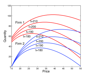
(a) Solutions with different values of $t$

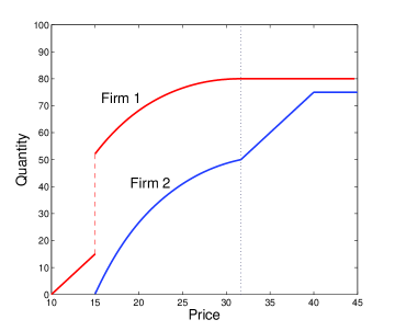
(b) Approximated SFE

Figure 5.1: Least squares approximation

Example 2.

This time we find the SFE in Example 1 with the general method. All the splines we use with the general method are B-splines. For this example, the knots are from 5 to 48 at step 0.05, and we put one price level at the center of each knot interval.

We solved (4.3) with IPOPT using the full monotonicity constraint, and obtained the optimal value $\rho=0.0048$, which is sufficiently close to 0. Figure 5.2 shows the spline approximation of the SFE. We see that when the mesh is fine enough, splines are quite capable at handling nonsmoothness and even discontinuities of the functions.

Comparing Figure 5.2 with Figure 5.1b, we see that both methods are able to find the equilibrium for markets of asymmetric duopoly with constant marginal costs, and the solutions are both of high precision. However, no matter in terms of the computational time, or in terms of the tools, solving a least squares problem is far easier than solving a highly nonlinear large scale optimization problem. Thus for this type of problems, the specialized least squares method is certainly more preferable.

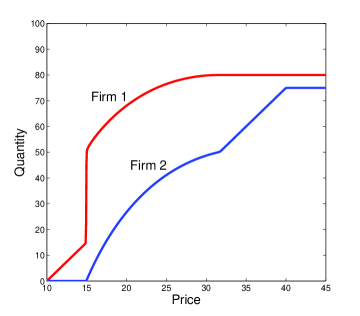
Figure 5.2: General method approximation

Example 3.

In this example we compare the effects of the two monotonicity constraints, and the results with different mesh sizes. The example is taken from Anderson and Hu [16], which has three firms with cost functions $C_{1}(q)=5q+0.8q^{2}$, $C_{2}(q)=8q+1.2q^{2}$ and $C_{3}(q)=12q+2.3q^{2}$, and capacities $Cap_{1}=11$, $Cap_{2}=8$ and $Cap_{3}=55$, respectively. The demand function is $D(p)=-0.5p+\varepsilon$.

First we compare the pointwise monotonicity with the full monotonicity constraints. The knots we use are from 5 to 54 at step 0.5, and we put a price level at the center of each knot interval. We solve the problem with CONOPT: The optimal value of $\rho$ is $1.6\times 10^{-10}$ if we use the pointwise constraint, and it is $0.002$ if we use the full constraint. Although the pointwise constraint gives a smaller $\rho$, it does not necessarily mean that it is the better choice. Figure 5.3 is a comparison of the results at the low price level, where images are magnified. Theoretically, we know that when $5\leq p<8$, Firm 1 is the monopoly, thus $s_{1}(p)=\frac{5}{18}(p-5)$, and we also know that $s_{1}$ should have a jump at $p=8$. We see that the solution given by the full constraint (5.3b) is closer to the true $s_{1}$ than the solution given by the pointwise constraint (5.3a) is. Therefore, despite a larger value of $\rho$, the full monotonicity constraint is in fact more robust.

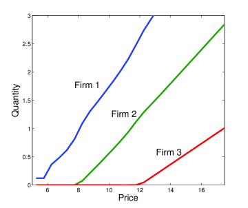
(a) pointwise monotonicity constraint

(b) full monotonicity constraint

Figure 5.3: Comparison of monotonicity constraints

We also see from Figure 5.3 that although the full monotonicity constraint gives a better approximation, it is still not close enough to the true equilibrium. This is due to the fineness of the mesh, and as we make the mesh finer, the result will be better. As an illustration, we reduce the knot interval from 0.5 to 0.1, and again put one price level at the center of each new knot interval. Keep the full monotonicity constraint and solve the problem, CONOPT gives a new result with $\rho=0.00017$. Figure 5.4 compares the result of the finer approximation (5.4b) with the previous coarser approximation (5.4a). It is apparent that the precision has significantly improved. Figure 5.5 is the full plot of the finer approximation for $5\leq p\leq 54$.

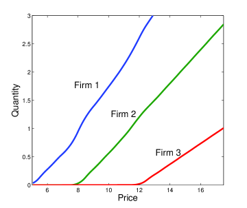
(a) $\left|\tau\right|=0.5$

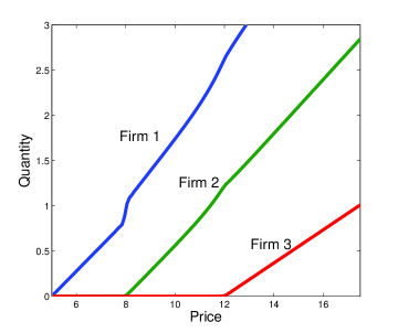
(b) $\left|\tau\right|=0.1$

Figure 5.4: Comparison of mesh sizes

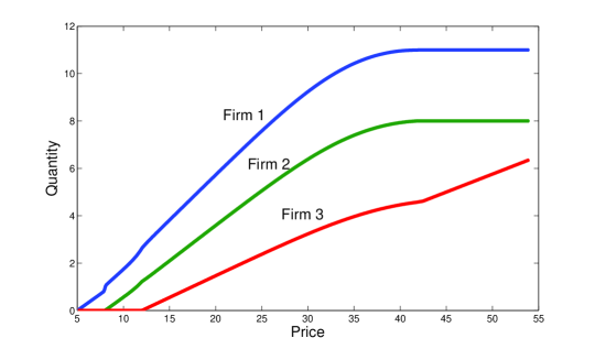
Figure 5.5: Approximation with $\left|\tau\right|=0.1$

For an even better approximation, one can always make the knot intervals smaller. However, as the number of knots increases, the problem will eventually become too large to solve. One way to improve the precision while keeping the problem size tractable is to use the information we obtained from a coarser approximation. From Figure 5.5 we can see that for $15\leq p\leq 40$, the supply functions are very smooth with little fluctuation, which means that a few pieces of quadratic polynomials are good enough to approximate them. Therefore we can, for example, set one knot at every 0.05 unit for $5\leq p\leq 15$, and at every 5 units for $15\leq p\leq 40$, which allows us to save hundreds of knots that would incur thousands of constraints.

6 Conclusions

One of the reasons why finding SFE has been so difficult is that the supply functions do not have specific forms, so all the non-decreasing functions (bounded by capacity) have to be considered. To find these free-form functions, parameterization is almost inevitable, and splines, due to their flexibility, are arguably the best way of parameterization for the purpose of approximation. For duopolies with constant marginal costs, we found that the first order conditions are linear in the spline coefficients, allowing us to approximate the solutions of the ODE system by solving a least squares problem. We proved that when the demand can be sufficiently low with a positive probability, the solution space of the least squares problem is exactly the solution space of the ODE system. And since least squares problems are so easy to solve, we can obtain solutions of high precision by using very fine mesh, while still solving it fast. The solutions have a clean form, which allows us to find the equilibrium easily by searching for the supply functions that reach the capacities smoothly.

We also used splines to improve the general purpose method given in Anderson and Hu [16]. Both their original method and our proposal should be equally accurate, but the use of splines enabled us to significantly reduce the number of decision variables and constraints used in the auxiliary NLP, thus making the problem easier to solve, and without the need of human intervention.

The solutions of both the specialized and the general purpose methods are proved to converge uniformly to the SFE. We also provided numerical examples to demonstrate the use of these methods, and the solutions are precise and reflect the theoretical properties of SFEs that we developed throughout the paper.

References

• [1] P.D. Klemperer, M.A. Meyer. Supply function equilibria in oligopoly under uncertainty. Econometrica, 57(6):1243–1277, 1989.
• [2] R.J. Green, D.M. Newbery. Competition in the British electricity spot market. The Journal of Political Economy, 100(5):929–953, 1992.
• [3] P. Holmberg. Unique supply function equilibrium with capacity constraints. Energy Economics, 30(1):148–172, 2008.
• [4] P. Holmberg. Supply function equilibrium with asymmetric capacities and constant marginal costs. The Energy Journal, 28(2):55–82, 2007.
• [5] A. Rudkevich, M. Duckworth, R. Rosen. Modeling electricity pricing in a deregulated generation industry: The potential for oligopoly pricing in a poolco. Energy Journal, 19(3):19–48, 1998.
• [6] R. Green. Increasing competition in the British electricity spot market. The Journal of Industrial Economics, 44(2):205–216, 1996.
• [7] R. Green. The electricity contract market in England and Wales. The Journal of Industrial Economics, 47(1):107–124, 1999.
• [8] R. Baldick, R. Grant, E. Kahn. Theory and application of linear supply function equilibrium in electricity markets. Journal of Regulatory Economics, 25(2):143–167, 2004.
• [9] P. Holmberg. Numerical calculation of an asymmetric supply function equilibrium with capacity constraints. European Journal of Operational Research, 199(1):285–295, 2009.
• [10] R. Baldick, W. Hogan. Capacity constrained supply function equilibrium models of electricity markets: stability, non-decreasing constraints, and function space iterations. 2001.
• [11] E.J. Anderson, A.B. Philpott. Using supply functions for offering generation into an electricity market. Operations Research, 50(3):477–489, 2002.
• [12] E.J. Anderson, A.B. Philpott. Optimal offer construction in electricity markets. Mathematics of Operations Research, 27(1):82–100, 2002.
• [13] E.J. Anderson, H. Xu. Necessary and sufficient conditions for optimal offers in electricity markets. SIAM Journal on Control and Optimization, 41(4):1212–1228, 2002.
• [14] A. Rudkevich. Supply function equilibrium: theory and applications. Proceedings of the 36th Annual Hawaii International Conference on System Sciences, strony 52–1. IEEE Computer Society, 2003.
• [15] R. Baldick, W. Hogan. Polynomial approximations and supply function equilibrium stability. 2004.
• [16] E.J. Anderson, X. Hu. Finding supply function equilibria with asymmetric firms. Operations Research, 56(3):697–711, 2008.
• [17] R. Sioshansi, S. Oren. How good are supply function equilibrium models: an empirical analysis of the ercot balancing market. Journal of Regulatory Economics, 31(1):1–35, 2007.
• [18] P. Holmberg, D.M. Newbery, D. Ralph. Supply function equilibria: Step functions and continuous representations. Cambridge Working Papers in Economics, 2008.
• [19] C. de Boor. A Practical Guide to Splines. Springer Verlag, 2001.
• [20] C.A. Hall. On error bounds for spline interpolation. Journal of Approximation Theory, 1(2):209–218, 1968.
• [21] C.A. Hall, W.W. Meyer. Optimal error bounds for cubic spline interpolation. Journal of Approximation Theory, 16(2):105–122, 1976.
• [22] E. Anderson. Supply function equilibria always exist. Working Paper, 2011.
• [23] M.J. Marsden. Quadratic spline interpolation. Bulletin of the American Mathematical Society, 80(5):903–906, 1974.
• [24] A. Wächter, L.T. Biegler. On the implementation of an interior-point filter line-search algorithm for large-scale nonlinear programming. Mathematical Programming, 106(1):25–57, 2006.
• [25] A.S. Drud. Conopt–a large-scale grg code. INFORMS Journal on Computing, 6(2):207, 1994.