Spectral Asymptotics for $V$-variable Sierpinski Gaskets

Abstract.

The family of $V$-variable fractals provides a means of interpolating between two families of random fractals previously considered in the literature; scale irregular fractals ($V=1$) and random recursive fractals ($V=\infty$). We consider a class of $V$-variable affine nested fractals based on the Sierpinski gasket with a general class of measures. We calculate the spectral exponent for a general measure and find the spectral dimension for these fractals. We show that the spectral properties and on-diagonal heat kernel estimates for $V$-variable fractals are closer to those of scale irregular fractals, in that it is the fluctuations in scale that determine their behaviour but that there are also effects of the spatial variability.

1. Introduction

The field of analysis on fractals has been primarily concerned with the construction and analysis of Laplace operators on self-similar sets. This has yielded a well developed theory for post critically finite (or p.c.f.) self-similar sets, a class of finitely ramified fractals [31]. One motivation for the development of such a theory, aside from its intrinsic mathematical interest, has come from the study of transport in disordered media. However, in this setting the fractals arise naturally in models from statistical physics at or near a phase transition and are therefore random objects without exact self-similarity but with some statistical self-similarity.

In order to develop the mathematical tools to tackle analysis on such random fractals one approach has been to work with simple models based on self-similar sets but exhibiting randomness. The first case to be treated was that of scale irregular fractals [17], [2], [24] and [11], which have spatial homogeneity but randomness in their scaling. A more natural setting is provided by random recursive fractals, initially constructed by [38], [12], [16], where the fractal can be decomposed into a random number of independent scaled copies. The study of some analytic properties of classes of random recursive Sierpinski gasket can be found in [18], [20] and [22].

Recently there has been work tackling random sets arising from critical phenomena directly, with a particular focus on the percolation model. Substantial progress has been made in the study of random walk on critical percolation clusters in the high dimensional case, see [3] and [36]. A bridge between these two approaches can be found in work on the continuum random tree [9], [10] or on critical percolation clusters on hierarchical lattices [23], both of which have random self-similar decompositions and hence have descriptions as random recursive fractals.

In this paper we consider $V$-variable fractals recently introduced in [6, 7]. This class of random fractals is defined via a family of iterated function systems and a positive integer parameter $V$. It interpolates between the class of homogeneous (scale irregular) random fractals, corresponding to $V=1$, and the class of random recursive fractals, corresponding to $V=\infty$. As for the random recursive fractals we can regard these $V$-variable fractals as determined by a probability measure on the set of labelled trees. In this case the measure is not a product measure, but is defined in a natural (if not completely obvious) manner which allows for at most $V$ distinct subtrees rooted at each level.

Our aim in this paper is to investigate the analytic properties of the class of $V$-variable Sierpinski gaskets and to compare their behaviour to the scale irregular and random recursive cases. We show their Hausdorff dimension in the resistance metric is the zero of a certain pressure function and their spectral dimension, the exponent for the growth of the eigenvalue counting function, is the zero of another pressure function. The connection between these two dimensions is established. We develop and extend standard methodology to examine more detailed properties of the eigenvalue counting function and the on-diagonal heat kernel. These results show that the $V$-variable fractals are closer to the scale irregular case, in that their fine properties are generally determined by fluctuations in scale rather than fluctuations which occur spatially across the fractal.

Model problems

We consider two model problems. Recall from [26] the description of a self-similar set as an iterated function system (or IFS) at each node of a tree generated by the address space.

Homogeneous and Random Recursive Fractals

For the first model problem we consider the two IFSs generating the Sierpinski gasket fractal SG(2) and the fractal SG(3) defined in [17]. The scale factors for SG(2) are mass $m_{2}=3$, length $\ell_{2}=2$ and time $s_{2}=5$. For SG(3) we have mass $m_{3}=6$, length $\ell_{3}=3$ and time $s_{3}=90/7$. The conductance scale factors can be computed directly, or from the Einstein relation $\rho=s/m$, giving $\rho_{2}=5/3,\rho_{3}=15/7$. Let $(M,S,L)$ be a triple of random variables taking each of the values $(m_{i},s_{i},\ell_{i})$ where $i=2,3$ with probabilities $p,1-p$ respectively.

Then, for the $V=1$ (homogeneous) case, we construct a random fractal using a sequence taking its values in $\{2,3\}$ and applying the corresponding IFS to all sets at a given level of construction. A realization of the first few stages can be seen in Figure 2. Then a simple scaling analysis shows that the Hausdorff dimension is given by $d_{f}=\mathbb{E}\log M/\mathbb{E}\log L$ where $\mathbb{E}$ denotes the expectation with respect to the probability measure generating the sequence. For the spectral dimension with respect to the natural “flat measure” one can extend the idea from [14] and [35] in the case of a single IFS fractal and apply a scaling argument to the Dirichlet form together with a Dirichlet-Neumann bracketing argument, see [19]. This gives the spectral dimension $d_{s}=2\mathbb{E}\log M/\mathbb{E}\log S$. For the $V=\infty$ (random recursive) case, each IFS is chosen independently for each node at each level. In this case we have $d_{s}=2d_{f}^{r}/(d_{f}^{r}+1)$ where $d_{f}^{r}$ is the Hausdorff dimension in the resistance metric, that is $d_{f}^{r}$ is such that $\mathbb{E}(M(S/M)^{-d_{f}^{r}})=\mathbb{E}M^{1+d_{f}^{r}}S^{-d_{f}^{r}}=1$. The argument again uses scaling properties of the Dirichlet form and a Dirichlet-Neumann bracketing argument, see [19, 20]. An alternative approach to computing the spectral dimension for random $V=1,\infty$ fractals is via heat kernel estimates, see [2] and [17, 18, 19, 20].

The second model problem is drawn from the class of affine nested fractals considered in [13]. This model interpolates between the slit triangle (which is not itself an affine nested fractal) and SG(3). Consider 7 triangles in the configuration shown in Figure 1 and take $\ell$ as the side length of the three triangles at the corners of the original triangle. The side lengths of the other triangles are given as $1-2\ell$ for the three triangles on the centre of each side and $3\ell-1$ for the downward pointing central triangle, where $1/3<\ell<1/2$. As $\ell\to 1/2$ we have the slit triangle and at $\ell=1/3$ we have SG(3).

Figure 1. A member of the family of Sierpinski gaskets interpolating SG(3) and the slit triangle, where $1/3<\ell<1/2$.

We construct a homogeneous random or random recursive fractal by taking a suitable distribution for $\ell$ on $[1/3,1/2)$ and either using a sequence, applying the same IFS at each node in the construction tree for the $V=1$ case, or independently for each node in the $V=\infty$ case.

We note that even scale irregular ($V=1$) affine nested gaskets of this type have not been treated before and as a consequence of our results we will be able to calculate the Hausdorff and spectral dimension for the random homogeneous version ($V=1$). By the triangle-star transform, if we assume that the resistance of each piece is proportional to its length, then the resistance scale factor is $(2\ell+1)/(\ell+2)$ in that if we take resistances on the three different types of triangle to be $(\ell+2)/(2\ell+1)(\ell,1-2\ell,3\ell-1)$ then this is electrically equivalent to the triangle with unit resistance on each edge.

In Section 2 we recall from [8] the Hausdorff dimension result for $V$-variable fractals, and we derive the spectral dimension from our calculations in Sections 4 and 5.

$V$-Variable Fractals

To understand the $V$-variable versions of our model problems, first consider the $V=1$ (spatially homogeneous, scale irregular) case of a $V$-variable labelled tree in a manner parallel to the approach taken in the general setting. See Figure 2. For $V=1$ all subtrees rooted at each fixed level are the same, as are the corresponding subfractals at each fixed level, hence the terminology “homogeneous”. The subtrees at one level are typically not the same as the subtrees at another level, hence the terminology “scale irregular”.

Figure 2. The level 3 approximation to a 1-variable tree, and the prefractal approximation to the associated 1-variable, or scale irregular, fractal. Here the family of IFSs is $\boldsymbol{F}=\{F(2),F(3)\}$ with members generating the sets $SG(2)$ and $SG(3)$ respectively.

For a general $V$-variable tree and for the corresponding $V$-variable fractal, there are at most $V$ distinct subtrees up to isomorphism rooted at each fixed level, and correspondingly at most $V$ distinct subfractals up to rescaling at each fixed level of refinement. See Figure 3 for a level 2 approximation to a $V$-variable tree with $V\geq 2$. In Section 2 we discuss this in some detail and see that there is a natural probability distribution on the class of $V$-variable fractals for each fixed $V$.

The construction of $V$-variable trees and hence $V$-variable fractals will require an assignment of a type chosen from $\{1,\dots,V\}$, as well as an IFS, to each node of the tree. Nodes with the same type and at the same level will have identical subtrees rooted at those nodes. The subfractals corresponding to those nodes will be identical up to scaling. See Figure 4. We choose the IFSs according to a probability measure and will write $P_{V}$ for the probability measure on the space of trees or $V$-variable fractals and $E_{V}$ for expectation with respect to $P_{V}$.

Let $n(1)$ be a random variable denoting the first level after level 0 at which all nodes are assigned the same type. Since the number of types is finite and we will assume a uniform upper bound on the branching number, $E_{V}n(1)<\infty$. Note that $n(1)=1$ if $V=1$, and clearly $E_{V}n(1)$ increases with $V$.

We write $\boldsymbol{i}=i_{1}\dots i_{k}$ for a node in the tree and denote its height or length by $|{\boldsymbol{i}}|=k$. The root node is denoted by $\emptyset$ and $|\emptyset|=0$. The Hausdorff dimension $d_{f}$ of the $V$-variable gasket formed from SG(2) and SG(3) is given $P_{V}$ almost surely by the zero of a pressure function in that ($P_{V}$ almost surely) it is the unique $d_{f}$ such that $E_{V}\log\sum_{|{\boldsymbol{i}}|=n(1)}(\ell_{i_{1}}\cdot\ldots\cdot\ell_{i_{n(1)}})^{d_{f}}=0$, where $\ell_{i_{k}}$ is the length scale value $1/2$ or $1/3$ according to which of SG(2) or SG(3) is chosen. See Theorem 2.17, also Theorem 2.18.

Results

For further detail see the Overview at the beginning of the following Sections 2–5.

Our main results first establish an expression for the spectral exponent over a general class of measures and determine the spectral dimension for these fractals. We then provide finer results of two types. We consider the eigenvalue counting function and the on-diagonal heat kernel and obtain upper and lower bounds on these quantities which hold for all $V$-variable trees. By placing a probability measure on the trees we obtain almost sure results capturing more explicitly their fluctuations. In the model problems the expectation is either over a discrete measure on $\{2,3\}$ or over a suitable distribution on $[1/3,1/2]$.

We show in Theorem 4.14 that the spectral exponent can also be expressed as the zero of a pressure function. In Theorems 4.16 and 4.18 we see that the spectral dimension, the maximum value of the spectral exponent over all measures $\mu$ defined using a product of weights, satisfies the equation $d_{s}/2=d_{f}^{r}/(d_{f}^{r}+1)$ where $d_{f}^{r}$ is the Hausdorff dimension in the resistance metric. This dimension in turn is the zero of another pressure function, see Theorem 3.11.

We establish upper and lower estimates for the eigenvalue counting function and on-diagonal heat kernel for a general class of measures. We show that the observed fluctuations arise from two different effects. The first is due to global scaling fluctuations as observed for scale irregular nested Sierpinski gaskets [2]. The second effect, which arises in the $V$-variable setting for $V>1$ or $V=1$ when the contraction factors are not all the same, gives additional, though much smaller, fluctuations due to the spatial variability of these fractals.

We first establish from Lemma 4.6 the non-probabilistic result that if ${\mathcal{N}}(\lambda)$ denotes the number of eigenvalues less than $\lambda$ (for the Dirichlet or Neumann Laplacian), then there is a time scale factor $T_{k}$, a mass scale factor $M_{k}$ and a correction factor $A_{k}$, such that there are constants $c_{1},c_{2}$ with

$$c_{1}M_{k}\leq\mathcal{N}(A_{k}T_{k})\mbox{ and }\mathcal{N}(T_{k})\leq c_{2}M_{k},\;\;\forall k.$$

As in the scale irregular gaskets of [2], this result is true for all realizations. By construction the scale factors $M_{k},T_{k}$ grow exponentially in $k$ but we will be able to show that $P_{V}$ almost surely we have $A_{k}\leq ck^{\beta}$, and even in certain cases $A_{k}\leq C(\log{k})^{\beta}$, for some constant $\beta$. The spectral exponent for any measure $\mu$ defined by a set of weights associated with a given IFS is

$$\frac{d_{s}(\mu)}{2}:=\lim_{x\to\infty}\frac{\log{\mathcal{N}(\lambda)}}{\log\lambda},$$

and we give a formula for this quantity as the zero of a suitable pressure function. In the case where the weights are ‘flat’ in the resistance metric we can show that there is a function $\phi(\lambda)=\exp(\sqrt{\log{\lambda}\log\log\log{\lambda}})$ such that $P_{V}$-almost surely

(1) $$c_{1}\lambda^{d_{s}/2}\phi(\lambda)^{-c_{2}}\leq\mathcal{N}(\lambda)\leq c_{3}\lambda^{d_{s}/2}\phi(\lambda)^{c_{4}},$$

for large $\lambda$, where $d_{s}=2d_{f}^{r}/(d_{f}^{r}+1)$ and $d_{f}^{r}$ is the Hausdorff dimension in the resistance metric.

To compare our results with previous work we note that in the $V=1$ case for nested Sierpinski gaskets it is shown in [2] that the Weyl limit for the normalized counting function does not exist in general and we have for all realizations that

$$c_{1}M_{k}\leq\mathcal{N}(T_{k})\leq c_{2}M_{k}.$$

This leads to the same size scale fluctuations as for the $V$-variable case given in (1). For the random recursive case of [20], the averaging leads to a Weyl limit in that

$$\lim_{\lambda\to\infty}\frac{\mathcal{N}(\lambda)}{\lambda^{d_{s}/2}}\text{ exists }\ P_{\infty}\;a.s.,$$

where $d_{s}=2d_{f}^{r}/(d_{f}^{r}+1)$ and $d_{f}^{r}$ is the Hausdorff dimension in the resistance metric.

We will also be able to remark on the on-diagonal heat kernel. We note that the measures we work with in this setting do not have the volume doubling property and hence it is harder work to produce good heat kernel estimates. In the setting considered here we can extend the arguments of [2] and [5] to get fluctuation results for the heat kernel. In Theorems 5.5 and  5.8 we show that the on-diagonal heat kernel estimate is determined by the local environment. In the case where the measure is the ‘flat’ measure in the resistance metric we can describe the small time global fluctuations in that for almost every point $x$ in the fractal,

$$c_{1}t^{-d_{s}/2}\phi(1/t)^{-c_{2}}\leq p_{t}(x,x)\leq c_{3}t^{-d_{s}/2}\phi(1/t)^{c_{4}},\;\;0<t\leq c_{5},\;\;P_{V}\;a.s.,$$

for suitable deterministic constants $c_{1},c_{2},c_{3},c_{4}$, and for all $t\leq c_{5}$, a random constant depending on the point $x$. These are of the same order as the $V=1$ case obtained in [2] and much larger than those in the random recursive case, [22].

In the case of general measures we will see that $P_{V}$-almost surely, $\mu$-almost every $x$ in the fractal does not have the same spectral exponent as the counting function (except when we choose the flat measure) and thus there will be a multifractal structure to the local heat kernel estimates in the same way as observed in [5], [21].

We restrict ourselves to affine nested fractals based on the Sierpinski gasket in $\mathbb{R}^{d}$ where $d\geq 2$. The problem of the existence of a limiting Dirichlet form is not solved more generally, even for the case of homogeneous random fractals. If this problem were solved, then the techniques used here would enable more general results to be obtained concerning $V$-variable p.c.f. fractals.

The structure of the paper is as follows. We give the construction of $V$-variable affine nested Sierpinski gaskets in Section 2. We show that by using the structure of $V$-variability there is a natural decomposition of the fractals at ‘necks’; a level at which all subtrees are the same. This idea was first used by Scealy in [39]. In Section 3 we construct the Dirichlet form, compute the resistance dimension, and determine other properties which will facilitate analysis on these sets. In Section 4 we treat the spectral asymptotics. The heat kernel is dealt with in Section 5.

Acknowledgement

We particularly wish to thank an anonymous referee for an unusually careful and detailed set of comments. Addressing these has led to a number of improvements in the results of the paper.

2. Geometry of $V$-Variable Fractals

2.1. Overview

Random $V$-variable fractals are generated from a possibly uncountable family $\boldsymbol{F}$ of IFSs. Each individual IFS $F\in\boldsymbol{F}$ generates an affine nested fractal. We also impose various probability distributions on $\boldsymbol{F}$.

For motivation, consider the two model problems in the Introduction. Namely, $\boldsymbol{F}=\{F_{2},F_{3}\}$ is the pair of IFSs generating $SG(2)$ and $SG(3)$, or $\boldsymbol{F}$ is the family of affine nested fractals $F_{\ell}$ generating the prefractal in Figure 1 for $\ell\in[1/3,1/2]$.

A $V$-variable tree corresponding to $\boldsymbol{F}$ is a tree with an IFS from $\boldsymbol{F}$ associated to each node, a type from the set $\{1,\dots,V\}$ associated to each node, and such that if two nodes at the same level have the same type, then the corresponding (labelled) subtrees rooted at those two nodes are isomorphic. This last requirement is achieved by using a sequence of environments, one at each level, to construct a $V$-variable tree. Each $V$-variable tree generates a $V$-variable fractal set in the natural way. The case $V=1$ corresponds to homogeneous fractals and $V\to\infty$ corresponds to random recursive fractals.

If all nodes at some level have the same type, the level is called a neck. Neck levels are given by a sequence of independent geometric random variables. In Lemma 2.15 we record some useful results for such random variables. In Section 2.7 we recall the Hausdorff dimension result from [8] but in the framework of necks as used in this paper, and then give a refinement by using the law of the iterated logarithm. This provides motivation for some of the spectral results.

2.2. Families of Affine Nested Fractals

Let ${\boldsymbol{F}}$ be a possibly uncountable class of IFSs $F$, each generating a compact fractal $K^{F}$, and each defined via a set of similitudes $\{\psi_{i}^{F}\}_{i\in S^{F}}$ acting on $\mathbb{R}^{d}$, with contraction factors $\{\ell_{i}^{F}\}_{i\in S^{F}}$ and $S^{F}=\{1,\dots,N^{F}\}$. If it is clear from the context we write $K$, $\psi_{i}$, $N$ and $S$ for $K^{F}$, $\psi_{i}^{F}$, $N^{F}$ and $S^{F}$ respectively, and similarly for other notation.

We will have

(2) $$\begin{gathered}3\leq N_{\inf}:=\inf\{N^{F}:F\in\boldsymbol{F}\}\leq\sup\{N^{F}:F\in\boldsymbol{F}\}=:N_{\sup}<\infty,\\ 0<\ell_{\inf}:=\inf\{\ell^{F}:F\in\boldsymbol{F}\}.\end{gathered}$$

The first follows from our later constructions, see (9). The second and third are for technical reasons arising in the study of the heat kernel and spectral asymptotics. See also the comments after Definition 2.14, from which it is clear that weaker conditions will suffice to construct $V$-variable fractals and establish their Hausdorff dimension.

Let $\Psi^{F}$ denote the set of fixed points of the $\{\psi_{i}^{F}\}_{i\in S^{F}}$. Then $x\in\Psi^{F}$ is an essential fixed point if there exists $y\in\Psi^{F}$ and $i\neq j$ such that $\psi_{i}^{F}(x)=\psi_{j}^{F}(y)$. Let $V_{0}$ denote the set of essential fixed points.

We always assume that $V_{0}$ does not depend on $F$.

Assume the uniform open set condition for the $\{\psi^{F}_{i}\}$. That is, there is a non-empty, bounded open set $O$, independent of $F$, such that $\{\psi^{F}_{i}(O)\}_{i\in S^{F}}$ are disjoint and $\bigcup_{i\in S^{F}}\psi_{i}^{F}(O)\subset O$.

Let $\psi^{F}_{i_{1}\cdots i_{n}}=\psi^{F}_{i_{1}}\circ\cdots\circ\psi^{F}_{i_{n}}$ and let

(3) $${V^{F}_{n}=\bigcup_{i_{1},\cdots,i_{n}\in S^{F}}\psi^{F}_{i_{1}\cdots i_{n}}(V_{0})},\quad V^{F}_{*}=\bigcup_{n\geq 0}V^{F}_{n}.$$

Then $K^{F}=cl(V^{F}_{*})$, the closure of $V^{F}_{*}$.

For $i_{1},\dots,i_{n}\in S^{F}$, we call $\psi^{F}_{i_{1}\cdots i_{n}}(V_{0})$ an $n$-cell and $\psi^{F}_{i_{1}\cdots i_{n}}(K^{F})$ an $n$-complex.

For $x,y\in{\mbox{$\mathbb{R}$}}^{d}(x\neq y)$, set $H_{xy}=\{z\in{\mbox{$\mathbb{R}$}}^{d}:|z-x|=|z-y|\}$ and let $U_{xy}:{\mbox{$\mathbb{R}$}}^{d}\to{\mbox{$\mathbb{R}$}}^{d}$ be the reflection transformation with respect to $H_{xy}$.

When computing the spectral dimensions we further assume each $K^{F}$ is an affine nested fractal. That is, the open set condition holds, $|V_{0}|\geq 2$, and:

1. $K^{F}$ is connected;

2. (Nesting) If $(i_{1},\cdots,i_{n})$ and $(j_{1},\cdots,j_{n})$ are distinct $n$-tuples of elements from $S^{F}$, then

   $$\psi^{F}_{i_{1}\cdots i_{n}}(K^{F})\cap\psi^{F}_{j_{1}\cdots j_{n}}(K^{F})=\psi^{F}_{i_{1}\cdots i_{n}}(V_{0})\cap\psi^{F}_{j_{1}\cdots j_{n}}(V_{0});$$

3. (Symmetry) For $x,y\in V_{0}~{}(x\neq y)$, $U_{xy}$ maps $n$-cells to $n$-cells, and it maps any $n$-cell which contains elements in both sides of $H_{xy}$ to itself for each $n\geq 0$.

We also make the technical assumption that $|\psi^{F}_{i}(V_{0})\cap\psi^{F}_{j}(V_{0})|\leq 1$ for all $1\leq i\neq j\leq N^{F}$.

2.3. Trees and Recursive Fractals

Fix a family ${\boldsymbol{F}}$ of IFSs as before. For our initial purposes it is sufficient only that the IFSs consist of uniformly contractive maps on $\mathbb{R}^{d}$.

Each realisation of a random fractal is built by means of an IFS construction tree, or tree for short, defined as follows.

Definition 2.1.

(See Figure 3) An (IFS construction) tree $T$ corresponding to $\boldsymbol{F}$ is a tree with the following properties:

1. there is a single, level 0, root node $\emptyset$;

2. the branching number $N^{\boldsymbol{i}}$ at each node $\boldsymbol{i}$ has $2\leq N^{\boldsymbol{i}}<\infty$ ($N^{\boldsymbol{i}}\geq 3$ later);

3. the edges with initial node $\boldsymbol{i}$ are numbered (“left to right”) by $1,\dots,N^{\boldsymbol{i}}$; where $\boldsymbol{i}=i_{1}\dots i_{k}$ in the usual manner and $|\boldsymbol{i}|:=k\geq 1$ is the level of $\boldsymbol{i}$, or $\boldsymbol{i}=\emptyset$ in which case $|\boldsymbol{i}|:=0$ is the level;

4. there is an IFS $F^{\boldsymbol{i}}\in\boldsymbol{F}$ associated with each node $\boldsymbol{i}$, $N^{\boldsymbol{i}}=|F^{\boldsymbol{i}}|$ (the cardinality of $F^{\boldsymbol{i}}$), and the $k$th edge with initial node $\boldsymbol{i}$ is associated with the $k$th function in the IFS $F^{\boldsymbol{i}}$.

The unique compact set $K=K(T)$ associated with $T$ in the usual manner is called a recursive fractal.

Figure 3. Level 2 approximations to an IFS tree and to the associated fractal. Here $\boldsymbol{F}=\{F(2),F(3)\}$ contains the IFSs generating $SG(2)$ and $SG(3)$ respectively. Edges of the tree with a given initial node are enumerated from left to right; they correspond to subcells enumerated anticlockwise from the bottom left corner of the cell corresponding to the given node.

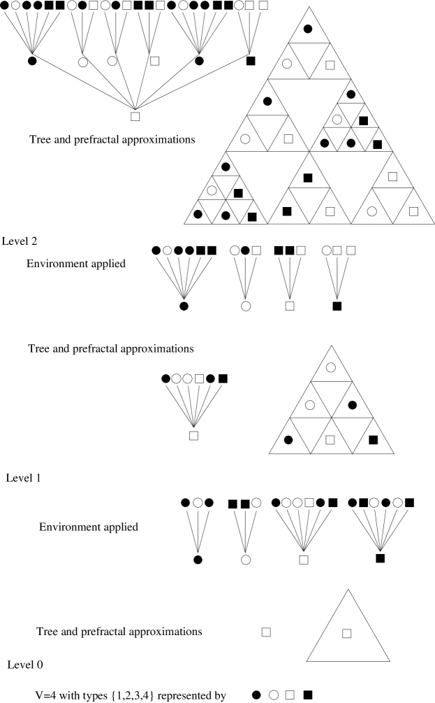
Figure 4. Approximations to a 4-variable tree and the prefractal approximations to the corresponding 4-variable fractal. The IFSs are $F(2)$ and $F(3)$ generating $SG(2)$ and $SG(3)$. The environment at each level is applied to the approximation at the previous level. The IFS labels are not shown since in this case they are determined by the branching number.

Notation 2.2.

The boundary $\partial T$ of a tree $T$ is the set of infinite paths through $T$ beginning at $\emptyset$.

For $\boldsymbol{i}\in T$ the cylinder set $[\boldsymbol{i}]\subset\partial T$ is the set of all infinite paths $\boldsymbol{w}\in\partial T$ such that $\boldsymbol{i}$ is an initial segment of $\boldsymbol{w}$, written $\boldsymbol{i}\prec\boldsymbol{w}$.

The concatenation of two sequences $\boldsymbol{i}$ and $\boldsymbol{j}$, where $\boldsymbol{i}$ is of finite length, is denoted by the juxtaposition $\boldsymbol{i}\boldsymbol{j}$.

The truncation of $\boldsymbol{i}$ to the first $n$ places is defined by $\boldsymbol{i}|n=i_{1}\dots i_{n}$.

A cut for the tree $T$ is a finite set $\Lambda\subset T$ with the property that for every $\boldsymbol{w}\in\partial T$ there is exactly one $\boldsymbol{i}\in\Lambda$ such that $\boldsymbol{i}\prec\boldsymbol{w}$. Equivalently, $\{[\boldsymbol{i}]:\boldsymbol{i}\in\Lambda\}$ is a partition of $\partial T$.

For a tree $T$ and a node $\boldsymbol{i}\in T$, there will usually be associated quantities such as an IFS $F^{\boldsymbol{i}}$, a type $\tau^{\boldsymbol{i}}\in\{1,\dots,V\}$ (see Definition 2.5) or a branching number $N^{\boldsymbol{i}}$. In this case $\boldsymbol{i}$ is shown as a superscript.

In particular, the transfer operator $\sigma^{\boldsymbol{i}}$ acts on $T$ to produce the tree $\sigma^{\boldsymbol{i}}T$, where, writing $T^{{\boldsymbol{j}}}$ for the address of node ${\boldsymbol{j}}$,

(4) $$\left(\sigma^{\boldsymbol{i}}T\right)^{\boldsymbol{j}}:=T^{\boldsymbol{i}\boldsymbol{j}}.$$

That is, $\sigma^{\boldsymbol{i}}T$ is the subtree of $T$ which has its base (or root) node at $\boldsymbol{i}$.

We frequently need to multiply a sequence of quantities, or compose a sequence of functions, along a finite branch corresponding to a node $\boldsymbol{i}=i_{1}\dots i_{n}$ of $T$. In this case, $\boldsymbol{i}$ is shown as a subscript. For example, if $\boldsymbol{i}=i_{1}\dots i_{n}$ then, with some abuse of notation for the second term,

(5) $$\ell_{\boldsymbol{i}}:=\ell_{i_{1}}\cdot\ldots\cdot\ell_{i_{n}}:=\ell^{F^{\emptyset}}_{i_{1}}\cdot\ell^{F^{i_{1}}}_{i_{2}}\cdot\ell^{F^{i_{1}i_{2}}}_{i_{3}}\cdot\ldots\cdot\ell^{F^{i_{1}\dots i_{n-1}}}_{i_{n}}$$

is the product of scaling factors corresponding to the edges along the branch $i_{1}\dots i_{n}$, and analogously for other scaling factors. Similarly,

(6) $$\psi_{\boldsymbol{i}}:=\psi_{i_{1}}\circ\dots\circ\psi_{i_{n}}:=\psi^{F^{\emptyset}}_{i_{1}}\circ\psi^{F^{i_{1}}}_{i_{2}}\circ\psi^{F^{i_{1}i_{2}}}_{i_{3}}\circ\dots\circ\psi^{F^{i_{1}\dots i_{n-1}}}_{i_{n}}$$

is the composition of functions along the same branch.

Notation 2.3 (Cells and Complexes).

The recursive fractal $K=K(T)$ generated by $T$ satisfies

(7) $$K(T)=\bigcup_{i=1}^{N^{\emptyset}}\psi_{i}^{F^{\emptyset}}\big{(}K(\sigma^{i}T)\big{)}=\bigcup_{|\boldsymbol{i}|=n}\psi_{\boldsymbol{i}}(K(\sigma^{\boldsymbol{i}}T)),$$

where the second equality comes from iterating the first.

For $|\boldsymbol{i}|=n$ the $n$-complex and $n$-cell with address $\boldsymbol{i}$ are respectively

(8) $$K_{\boldsymbol{i}}=\psi_{\boldsymbol{i}}(K(\sigma^{\boldsymbol{i}}T)),\quad\Delta_{\boldsymbol{i}}:=\psi_{\boldsymbol{i}}(V_{0}),$$

recalling that $V_{0}$ is the set of essential fixed points of $F\in\boldsymbol{F}$ and is the same for all  $F$.

Assumption 2.4.

In Section 3 and subsequently we assume

(9) $$\text{$V_{0}$ is the set of vertices of an equilateral tetrahedron in $\mathbb{R}^{d}$ for some $d\geq 2$},$$

$$\text{$E_{0}$ is the set of edges},G_{0}=(V_{0},E_{0})\text{ is the complete graph on }V_{0}.$$

We will need various sequences of graph approximations $\{G_{n}\}_{n=0}^{\infty}$ to the fractal $K(T)$. In particular we use the notation $G_{n}=(V_{n},E_{n})$, where

(10) $$V_{n}:=\bigcup_{|\boldsymbol{i}|=n}\psi_{\boldsymbol{i}}(V_{0})=\bigcup_{|\boldsymbol{i}|=n}\Delta_{\boldsymbol{i}},\quad E_{n}:=\bigcup_{|\boldsymbol{i}|=n}\psi_{\boldsymbol{i}}(E_{0}).$$

We can recover the fractal itself as $K(T)=cl(\bigcup_{n}V_{n})$, where $cl$ denotes closure.

We will write $x\sim_{n}y$ for $x,y\in V_{n}$ if $x,y$ are connected by an edge in $E_{n}$.

2.4. $V$-Variable Trees and $V$-Variable Fractals

Fix a natural number $V$. For motivation see Figure 4.

The following definition of a $V$-variable tree and $V$-variable fractal is equivalent to that in [7] and [8], but avoids working with $V$-tuples of trees and fractals.

Definition 2.5.

A $V$-variable tree corresponding to $\boldsymbol{F}$ is an IFS construction tree $T$ corresponding to $\boldsymbol{F}$, with a type $\tau^{\boldsymbol{i}}\in\{1,\dots,V\}$ associated to each node $\boldsymbol{i}$. Moreover, if two nodes $\boldsymbol{i}$ and $\boldsymbol{j}$ at the same level $|\boldsymbol{i}|=|\boldsymbol{j}|$ have the same type $\tau^{\boldsymbol{i}}=\tau^{\boldsymbol{j}}$, then:

1. $\boldsymbol{i}$ and $\boldsymbol{j}$ have the same associated IFS $F^{\boldsymbol{i}}=F^{\boldsymbol{j}}$ and hence the same branching number $N^{\boldsymbol{i}}=N^{\boldsymbol{j}}$;

2. comparable successor nodes $\boldsymbol{i}p$ and $\boldsymbol{j}p$, where $1\leq p\leq N^{\boldsymbol{i}}=N^{\boldsymbol{j}}$, have the same type $\tau^{\boldsymbol{i}p}=\tau^{\boldsymbol{j}p}$.

The recursive fractal $K=K(T)$ associated to a $V$-variable tree $T$ as above is called a $V$-variable fractal corresponding to $\boldsymbol{F}$.

The class of $V$-variable trees and class of $V$-variable fractals corresponding to $\boldsymbol{F}$ are denoted by $\Omega_{V}=\Omega^{\boldsymbol{F}}_{V}$ and $\mathcal{K}_{V}=\mathcal{K}^{\boldsymbol{F}}_{V}$ respectively.

Remark 2.6.

A $V$-variable tree has at most $V$ distinct IFSs associated to the nodes at each fixed level. If two nodes at the same level of a $V$-variable tree have the same type then the subtrees rooted at these two nodes are identical, i.e.

(11) $$|\boldsymbol{i}|=|\boldsymbol{j}|\ \&\ \tau^{\boldsymbol{i}}=\tau^{\boldsymbol{j}}\ \Longrightarrow\ \sigma^{\boldsymbol{i}}T=\sigma^{\boldsymbol{j}}T.$$

In particular, for each level, there are at most $V$ distinct subtrees rooted at that level.

A 1-variable tree is essentially the same as an IFS tree which generates a scale irregular or homogeneous fractal as in [17], [19] and [2].

The following is used in the construction and analysis of $V$-variable fractals.

Definition 2.7.

An environment $E$ assigns to each type $v\in\{1,\dots,V\}$ both an IFS $F_{v}\in\boldsymbol{F}$ and a sequence of types $(\tau_{v,i})_{i=1}^{|F_{v}|}$, where $|F_{v}|$ is the number of functions in $F_{v}$. We write

(12) $$E=\big{(}E(1),\dots,E(V)\big{)},\quad E(v)=\big{(}F^{E}_{v},\tau^{E}_{v,1},\dots,\tau^{E}_{v,|F_{v}|}\big{)}.$$

For a pictorial example see Figure 4. For the following consider the case $n=2$ in Figure 4.

Construction 2.8.

A $V$-variable tree is constructed from a sequence of environments $(E^{k})_{k\geq 1}$ in the natural way as follows:

• Begin with the root node $\emptyset$ and an initial type $\tau^{\emptyset}$ assigned to this node.

• Use $E^{1}$ and the type $\tau^{\emptyset}$ in the natural way to assign an IFS to the level 0 node, construct the level 1 nodes and assign a type to each of them.

  More precisely, use $E^{1}(v)$ where

  $$v:=\tau^{\emptyset},\quad E^{1}\big{(}v\big{)}=\Big{(}F^{E^{1}}_{v},\tau^{E^{1}}_{v,1},\dots,\tau^{E^{1}}_{v,|F^{E^{1}}_{v}|}\Big{)},$$

  to assign the IFS $F^{\emptyset}:=F^{E^{1}}_{v}$ to the node $\emptyset$ and in particular determine the branching number $N^{\emptyset}:=\big{|}F^{E^{1}}_{v}\big{|}$ at $\emptyset$, and to assign the type $\tau^{j}:=\tau^{E^{1}}_{v,j}$ to each level $1$ node $j$.

• (By the completion of stage $n-1$ for $n\geq 2$, an IFS $F^{\boldsymbol{i}}$ will have been assigned to each node $\boldsymbol{i}$ of level $|\boldsymbol{i}|\leq n-2$, all nodes $\boldsymbol{i}$ of level $|\boldsymbol{j}|\leq n-1$ will have been constructed and a type $\tau^{\boldsymbol{j}}$ will have been assigned to each.)

  Use $E^{n}$ in the natural way to assign an IFS to each level $n-1$ node according to its type, to construct the level $n$ nodes and to assign a type to them.

  More precisely, use $E^{n}(v)$ for $1\leq v\leq V$ where

  $$E^{n}\big{(}v\big{)}=\Big{(}F^{E^{n}}_{v},\tau^{E^{n}}_{v,1},\dots,\tau^{E^{n}}_{v,|F^{E^{n}}_{v}|}\Big{)},$$

  to assign the IFS $F^{\boldsymbol{i}}:=F^{E^{n}}_{v}$ to each level $n-1$ node $\boldsymbol{i}$ of type $v$ and in particular to determine the branching number $N^{\boldsymbol{i}}:=\big{|}F^{E^{n}}_{v}\big{|}$ at the node $\boldsymbol{i}$, and to assign the type $\tau^{\boldsymbol{i}j}:=\tau^{E^{n}}_{v,j}$ to the level $n$ node $\boldsymbol{i}j$.

It follows by an easy induction that the properties in Definition 2.5 hold at all nodes. $\square$

We now note the following facts about the connectivity properties of $V$-variable fractals.

Lemma 2.9.

Let $K$ be a $V$-variable fractal. Then
(1) $K$ is connected
(2) $K$ is nested: For all ${\boldsymbol{i}},{\boldsymbol{j}}\in T$, if $[{\boldsymbol{i}}]\cap[{\boldsymbol{j}}]=\emptyset$, then $K_{{\boldsymbol{i}}}\cap K_{{\boldsymbol{j}}}=\psi_{{\boldsymbol{i}}}(V_{0})\cap\psi_{{\boldsymbol{j}}}(V_{0})$.

Proof.

(1) The connectedness is clear as all the affine nested fractals in the family are connected.

(2) In our setting this is straightforward to see as if $[{\boldsymbol{i}}]\cap[{\boldsymbol{j}}]=\emptyset$, there exists a ${\boldsymbol{k}}$ of maximal length with ${\boldsymbol{k}}\prec{\boldsymbol{i}}$ and ${\boldsymbol{k}}\prec{\boldsymbol{j}}$, such that $K_{{\boldsymbol{i}}}\subset K_{{\boldsymbol{k}}}$ and $K_{{\boldsymbol{j}}}\subset K_{{\boldsymbol{k}}}$. If we write ${\boldsymbol{i}}={\boldsymbol{k}}i_{1}\dots$ and ${\boldsymbol{j}}={\boldsymbol{k}}j_{1}\dots$, then $i_{1}\neq j_{1}$ and by the nesting axiom for $F^{{\boldsymbol{k}}}$ we have $K_{{\boldsymbol{k}}i_{1}}\cap K_{{\boldsymbol{k}}j_{1}}=\psi_{{\boldsymbol{k}}i_{1}}(V_{0})\cap V_{{\boldsymbol{k}}j_{1}}(V_{0})$. If the intersection is empty we are done. Otherwise, by our technical assumption on affine nested fractals that $|\psi^{F^{{\boldsymbol{k}}}}_{i_{1}}(V_{0})\cap\psi^{F^{{\boldsymbol{k}}}}_{j_{1}}(V_{0})|\leq 1$, there is a single intersection point which is the image of a fixed point in $V_{0}$. If $K_{{\boldsymbol{i}}}\cap K_{{\boldsymbol{j}}}\neq\emptyset$, this is the intersection point of $K_{{\boldsymbol{i}}}\cap K_{{\boldsymbol{j}}}$ and therefore of $\psi_{{\boldsymbol{i}}}(V_{0})\cap V_{{\boldsymbol{j}}}(V_{0})$ as required. If $K_{{\boldsymbol{i}}}\cap K_{{\boldsymbol{j}}}=\emptyset$ we are done. ∎

2.5. Random $V$-Variable Trees and Random $V$-Variable Fractals

Definition 2.10.

Fix a probability distribution $P$ on $\boldsymbol{F}$. This induces a probability distribution $P_{V}$ on the set of environments as follows. Choose the IFSs $F^{{E}}_{v}$ for $v\in\{1,\dots,V\}$ in an i.i.d. manner according to $P$. Choose types $\tau^{{E}}_{v,j}$ for $1\leq j\leq|F^{{E}}_{v}|$ in an i.i.d. manner according to the uniform distribution on $\{1,\dots,V\}$ and otherwise independently of the $F^{{E}}_{w}$.

Definition 2.11.

The probability distribution on the set $\Omega_{V}$ of $V$-variable trees is obtained by choosing $\tau^{\emptyset}\in\{1,\dots,V\}$ according to the uniform distribution and independently choosing the environments at each stage in an i.i.d. manner according to $P_{V}$. This probability distribution on $V$-variable trees induces a probability distribution on the set $\mathcal{K}_{V}$ of $V$-variable fractals. Both the probability distribution on trees and that on fractals are denoted by $P_{V}$. We will write $E_{V}$ for expectation with respect to $P_{V}$.

Random $V$-variable trees and random $V$-variable fractals are random labelled trees and random compact subsets of $\mathbb{R}^{d}$ respectively, having the distribution $P_{V}$. Later, when we add additional scale factors for resistance and weights associated with each $F\in\boldsymbol{F}$, we will assume they are measurable with respect to $F\in\boldsymbol{F}$.

Although the distribution $P_{V}$ on environments is a product measure, this is far from the case for the corresponding distribution $P_{V}$ on $\Omega_{V}$ and $\mathcal{K}_{V}$. There is a high degree of dependency between the types (and hence the IFSs) assigned to different nodes at the same level.

Remark 2.12.

The classes $\mathcal{K}_{V}$ interpolate between the class of homogeneous fractals in the case $V=1$ and the class of recursive fractals as $V\to\infty$. The probability spaces $(\mathcal{K}_{V},P_{V})$ interpolate between the natural probability distribution on homogeneous fractals in the case $V=1$ and the natural probability distribution on the class of recursive fractals as $V\to\infty$. See [6] and [7].

Notation 2.13.

It will often be convenient to identify the sample space for random quantities such as trees, fractals, functions associated to a branch of a tree, etc., with the set $\Omega_{V}$ of $V$-variable trees. We use $\omega$ to denote a generic element of $\Omega_{V}$ and combine this with other notations in the natural manner. Thus we may write $T^{\omega}$, $K^{\omega}$, $\psi_{\boldsymbol{i}}^{\omega}$ etc.

In particular, $\sigma^{\boldsymbol{i}}\omega$ is the transfer operator defined in Notation 2.2 for a tree $T$. See for example the first equality in (28). However, we usually suppress $\omega$ as in the second equation in (28). Also see (90) and the explanation which follows it.

2.6. Necks

The notion of a neck is critical for the analysis that follows.

Definition 2.14.

The environment $E$ in Definition 2.7 is a neck if all $\tau_{v,i}^{E}$ are equal.

A neck for a $V$-variable tree $\omega$ is a natural number $n$ such that the environment $E$ applied at stage $n$ in the construction of $\omega$ is a neck environment. In this case we say a neck occurs at level $n$. If $\boldsymbol{i}$ is a node in $\omega$ and $|\boldsymbol{i}|=n$, then $\boldsymbol{i}$ is called a level $n$ neck node.

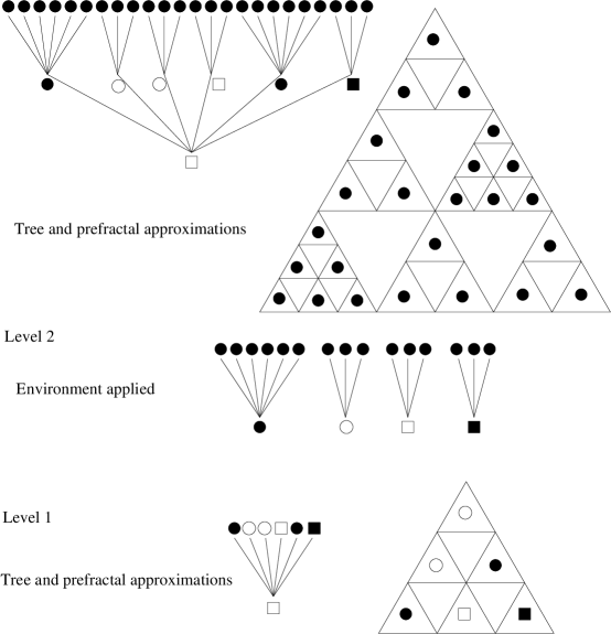
Figure 5. Compare with Figure 4, except that now a neck occurs at level 2. All subtrees rooted at this level will be the same, although they have not yet been constructed. All 2-complexes will be the same up to scaling by factors determined by the construction up to this level.

If a neck occurs at level $n$ then the type assigned to every node at that level is the same. See Figure 5. It follows from Remark 2.6 that all subtrees rooted at level $n$ will be the same. Note that the subtrees themselves are only constructed at later stages, and even the common value of the IFS at a level $n$ neck node is not determined until stage $n+1$.

There is however no restriction on the IFSs occurring in a neck environment ${E}$. For a level $n$ neck these IFSs are applied at level $n-1$.

Because there is an upper bound on the number of functions $N^{F}$ in any IFS $F\in\boldsymbol{F}$, there is only a finite number of type choices to be made in selecting an environment. It follows that necks occur infinitely often almost surely with respect to the probability $P_{V}$ defined in Definition 2.11. The sequence of neck levels in the construction of a $V$-variable tree or fractal is denoted by

(13) $$0=n(0)<n(1)<\dots<n(k)<\cdots.$$

The sequence of times between necks is a sequence of independent geometric random variables, and in particular the expected first neck satisfies

(14) $$E_{V}n(1)<\infty.$$

Many of our future estimates rely on various a.s. properties of necks. However, some estimates just require that there be an infinite sequence of necks. For this reason we make the definition:

(15) $$\Omega^{\prime}_{V}\subset\Omega_{V} V$$ is the set of -variable trees with an infinite sequence of necks.

We next give an elementary result on the asymptotic behaviour of a sequence of geometric random variables $(Y_{k})_{k\geq 1}$. It follows that $Y_{k}$ grows at most logarithmically in $k$, and powers of $Y_{k}$ grow at most geometrically, with similar results for the maximum and the mean of $\{Y_{1},\dots,Y_{k}\}$.

The following is standard but included for completeness. Note that the $Y_{k}$ need not actually be geometric random variables.

Lemma 2.15.

Suppose $\{Y_{k}\}_{k=1}^{\infty}$ is a sequence of not necessarily independent random variables with $P(Y_{k}>x)\leq Ap^{x}$, where $0<p<1$ and for all $x>0$. Suppose $n\geq 1$ is a natural number. Then a.s.

(16) $$\limsup_{k\to\infty}\frac{Y_{nk}}{\log{k}}\leq\frac{1}{\log 1/p},\quad\limsup_{k\to\infty}\frac{\max_{1\leq i\leq nk}Y_{i}}{\log{k}}\leq\frac{1}{\log 1/p},$$

(17) $$\limsup_{k\to\infty}\frac{\sum_{i=1}^{nk}Y_{i}}{k\log k}\leq\frac{2n}{\log 1/p}.$$

Proof.

The case $n>1$ is a direct consequence of the case $n=1$, which we establish.

Suppose $\epsilon>0$. Since $P(Y_{k}>x)\leq Ap^{x}$ for $x>0$,

$$\sum_{k\geq 1}P\left(Y_{k}>\frac{(1+\epsilon)\log k}{\log 1/p}\right)\leq A\sum_{k\geq 1}p^{(1+\epsilon)\log k/(\log 1/p)}=A\sum_{k\geq 1}k^{-(1+\epsilon)}<\infty.$$

Hence by the first Borel-Cantelli lemma,

$$\limsup_{k\to\infty}\frac{Y_{k}}{\log{k}}\leq\frac{1+\epsilon}{\log 1/p}\text{\quad a.s.}$$

Since $\epsilon>0$ is arbitrary, the first inequality in (16) follows.

The second inequality in (16) is now an elementary consequence. Suppose $\delta>0$. Using the first inequality in (16) to get the second inequality below, $P$ a.s. there exists $k_{0}=k_{0}(\omega,\delta)$ such that $k\geq k_{0}$ implies

$$\max_{k_{0}\leq i\leq k}\frac{Y_{i}}{\log{k}}\leq\max_{k_{0}\leq i\leq k}\frac{Y_{i}}{\log i}\leq\frac{1}{\log 1/p}+\delta.$$

Hence

$$\limsup_{k\to\infty}\max_{k_{0}\leq i\leq k}\frac{Y_{i}}{\log{k}}\leq\frac{1}{\log 1/p}+\delta\text{\quad a.s.}$$

Replacing $k_{0}$ by $1$ and letting $\delta\to 0$ in the above implies the second inequality in (16).

For (17) fix $\gamma>0$. Then

$$\sum_{k\geq 1}P\Bigg{(} \sum_{i=1}^{k}Y_{i}>\frac{\gamma k\log k}{\log 1/p}\Bigg{)}\leq\sum_{k\geq 1}\sum_{i=1}^{k}P\left(Y_{i}>\frac{\gamma\log k}{\log 1/p}\right)$$

$$\leq\sum_{k\geq 1}kAp^{\gamma\log k/\log 1/p}=A\sum_{k\geq 1}k^{1-\gamma}<\infty,\text{ if }\gamma>2.$$

By the first Borel-Cantelli lemma, if $\gamma>2$,

$$\limsup_{k\to\infty}\frac{\sum_{i=1}^{k}Y_{i}}{k\log k}\leq\frac{\gamma}{\log 1/p}\quad\text{a.s}.$$

This gives (17). ∎

We also include a decomposition of sums of products of scale factors.

It may help to note that the factors on the right side of (19) in the next Lemma are calculated by first choosing and fixing, for each $j=1\dots k$, an arbitrary node of $T$ at level $n(j-1)$. For fixed $j$ all subtrees of $T$ rooted at this level are identical by the definition of a neck. The factor in (19) is the sum, of products of $s_{i}^{p}$ type weights, along all paths in such a subtree starting from its root node and ending at a first neck level node. There is a one-one correspondence between the set of such paths in the subtree and the set of paths in the original tree starting from the chosen node at level $n(j-1)$ and ending at a level $n(j)$ node.

Lemma 2.16.

Let $s_{i}=s_{i}^{F}\in\mathbb{R}$ for $i=1,\dots,N^{F}$ be scaling factors associated with each family $F$, where

(18) $$0<s_{\inf} :=\inf\{s^{F}_{i}:i\in 1,\dots,N^{F},\,F\in{\boldsymbol{F}}\},$$

$$s_{\sup} :=\sup\{s^{F}_{i}:i\in 1,\dots,N^{F},\,F\in\boldsymbol{F}\}<\infty.$$

Then, writing $s_{{\boldsymbol{i}}}=s_{i_{1}}\cdot\ldots\cdot s_{i_{n}}$ for ${\boldsymbol{i}}=i_{1}\dots i_{n}\in T$, and with $s^{(j)}_{\boldsymbol{i}}$ defined in the natural way in the body of the proof, we have

(19) $$\sum_{\boldsymbol{i}\in T,|\boldsymbol{i}|=n(k)}s_{\boldsymbol{i}}=\prod_{j=1}^{k}\Bigg{(}\sum_{|\boldsymbol{i}|=n(j)-n(j-1)}s^{(j-1)}_{\boldsymbol{i}}\Bigg{)}.$$

Moreover,

(20) $$\lim_{k\to\infty}\frac{1}{k}\log\sum_{|\boldsymbol{i}|=n(k)}s_{\boldsymbol{i}}=E_{V}\log\sum_{|\boldsymbol{i}|=n(1)}s_{\boldsymbol{i}}\quad P_{V}\text{ a.s.}$$

Proof.

Let $T^{(k)}$ denote the unique subtree of $T$ rooted at the neck level $n(k)$, so that in particular $T^{(0)}=T$.

Then, as explained subsequently (and following the notation of (5) but with the $F$ there suppressed),

$$\sum_{\boldsymbol{i}\in T,|\boldsymbol{i}|=n(k)}s_{\boldsymbol{i}}=\sum_{\boldsymbol{i}\in T,|\boldsymbol{i}|=n(k)}s_{i_{1}}^{\emptyset}\cdot s_{i_{2}}^{i_{1}}\cdot s_{i_{3}}^{i_{1}i_{2}}\cdot\ldots\cdot s_{i_{n(k)}}^{\boldsymbol{i}|(n(k)-1)}$$

$$\qquad=\sum_{\boldsymbol{i}\in T,|\boldsymbol{i}|=n(k)}\bigg{\{}\left(s_{i_{1}}^{\emptyset}\cdot s_{i_{2}}^{i_{1}}\cdot s_{i_{3}}^{i_{1}i_{2}}\cdot\ldots\cdot s_{i_{n(1)}}^{\boldsymbol{i}|(n(1)-1)}\right)$$

$$\qquad\qquad\qquad\quad\cdot\left(s_{i_{n(1)+1}}^{\boldsymbol{i}|n(1)}\cdot s_{i_{n(1)+2}}^{\boldsymbol{i}|n(1)+1}\cdot\ldots\cdot s_{i_{n(2)}}^{\boldsymbol{i}|(n(2)-1)}\right)\cdot\ldots$$

$$\qquad\qquad\qquad\quad\cdot\left(s_{i_{n(k-1)+1}}^{\boldsymbol{i}|n(k-1)}\cdot s_{i_{n(k-1)+2}}^{\boldsymbol{i}|n(k-1)+1}\cdot\ldots\cdot s_{i_{n(k)}}^{\boldsymbol{i}|(n(k)-1)}\right)\bigg{\}}$$

$$\qquad=\sum_{\boldsymbol{i}\in T^{(0)},|\boldsymbol{i}|=n(1)}s_{i_{1}}^{(0),\emptyset}\cdot s_{i_{2}}^{(0),i_{1}}\cdot s_{i_{3}}^{(0),i_{1}i_{2}}\cdot\ldots\cdot s_{i_{n(1)}}^{(0),\boldsymbol{i}|(n(1)-1)}$$

$$\quad\times\sum_{\boldsymbol{i}\in T^{(1)},|\boldsymbol{i}|=n(2)-n(1)}s_{i_{1}}^{(1),\emptyset}\cdot s_{i_{2}}^{(1),i_{1}}\cdot s_{i_{3}}^{(1),i_{1}i_{2}}\cdot\ldots\cdot s_{i_{n(2)-n(1)}}^{(1),\boldsymbol{i}|(n(2)-n(1)-1)}\cdot\ldots$$

$$\quad\times\sum_{\boldsymbol{i}\in T^{(k-1)},|\boldsymbol{i}|=n(k)-n(k-1)}s_{i_{1}}^{(k-1),\emptyset}\cdot s_{i_{2}}^{(k-1),i_{1}}\cdot s_{i_{3}}^{(k-1),i_{1}i_{2}}\cdot\ldots\cdot s_{i_{n(k)-n(k-1)}}^{(k-1),\boldsymbol{i}|(n(k)-n(k-1)-1)}$$

(21) $$=\Bigg{(}\sum_{|\boldsymbol{i}|=n(1)}s^{(0)}_{\boldsymbol{i}}\Bigg{)}\cdot\Bigg{(}\sum_{|\boldsymbol{i}|=n(2)-n(1)}s^{(1)}_{\boldsymbol{i}}\Bigg{)}\cdot\ldots\cdot\Bigg{(}\sum_{|\boldsymbol{i}|=n(k)-n(k-1)}s^{(k-1)}_{\boldsymbol{i}}\Bigg{)}.$$

The first and last equality are immediate from the definitions. The second equality is just a bracketing of terms.

For the third equality note that each $n(j)$ is a neck. A term such as $s_{i_{n(1)+1}}^{\boldsymbol{i}|n(1)}$, which corresponds to the edge in $T$ from $\boldsymbol{i}|n(1)=i_{1}\dots i_{n(1)}$ to $i_{1}\dots i_{n(1)}i_{n(1)+1}$, is independent of $\boldsymbol{i}|n(1)$ and can also be regarded as corresponding to the level one edge from $\emptyset$ to $i_{n(1)+1}$ of the unique tree $T^{(1)}$ rooted at every level $n(1)$ node. Thus we rewrite $s_{i_{n(1)+1}}^{\boldsymbol{i}|n(1)}$ as $s_{i_{1}}^{(1),\emptyset}$, with an abuse of notation in that $\boldsymbol{i}$ and $i_{n(1)+1}$ in the first term refer to words from $T=T^{(0)}$ whereas $i_{1}$ in the second term is the first element of a word from $T^{(1)}$. Similarly, $s_{i_{n(1)+2}}^{\boldsymbol{i}|n(1)+1}$ is also independent of $\boldsymbol{i}|n(1)$ and can also be regarded as corresponding to a level two edge from $T^{(1)}$, etc. Now use simple algebra to put the summations inside the parentheses.

The final equality is a rewriting of the previous line and provides the definition of $s^{(j)}_{\boldsymbol{i}}$.

For the $P_{V}$ almost sure convergence in (20) let

$$X_{k}=\log\sum_{|\boldsymbol{i}|=n(k)-n(k-1)}s^{(k-1)}_{\boldsymbol{i}},\ k\geq 1.$$

By construction the $X_{k}$ are i.i.d. and in particular $X_{1}=\log\sum_{|\boldsymbol{i}|=n(1)}s_{\boldsymbol{i}}$. By the bounds on $s_{i}$ we have

$$E_{V}|X_{1}| \leq\sum_{n\geq 1}P\big{(}n(1)=n\big{)}\,\max\Big{\{}\big{|}\log\big{(}N_{\sup}^{n}s_{\sup}^{n}\big{)}\big{|},\ \big{|}\log\big{(}N_{\inf}^{n}s_{\inf}^{n}\big{)}\big{|}\Big{\}}$$

$$=\max\Big{\{}\big{|}\log\big{(}N_{\sup}s_{\sup}\big{)}\big{|},\,\big{|}\log\big{(}N_{\inf}s_{\inf}\big{)}\big{|}\Big{\}}E_{V}n(1)<\infty.$$

Hence, using (19), the $P_{V}$ almost sure convergence follows from the strong law of large numbers for the sequence $\{X_{k}\}$. ∎

2.7. Hausdorff and Box Dimensions

Assume that the family of IFSs ${\boldsymbol{F}}$ satisfies the open set condition as in Section 2.2. We do not here require the affine nested condition. Recall the notation from Section 2.2 and from Notation 2.2.

Splitting up and treating the necks in the manner here was done first by Scealy in his PhD thesis [39].

Theorem 2.17.

Suppose $K$ is the random $V$-variable fractal generated from $\boldsymbol{F}$. Then the Hausdorff and box dimension of $K$ is $P_{V}$ a.s. given by the unique $\alpha$ such that

(22) $$E_{V}\log\sum_{|{\boldsymbol{i}}|={n(1)}}{\ell_{\boldsymbol{i}}}^{\alpha}=0.$$

Proof.

See the Main Theorem in Section 4.4 of [8]. The expression there for the pressure function is equal to the simpler expression here. This in turn leads to a simpler proof of that theorem, still along the lines of Lemma 5.7 in [8] but working with a single neck as in the (somewhat more complicated) proofs of Theorems 3.11 and 4.14. ∎

We give a slight refinement of this result.

Theorem 2.18.

There exists a constant $C$ such that

(23) $$\limsup_{k\to\infty}\frac{1}{\sqrt{k\log{\log{k}}}}\log\sum_{|\boldsymbol{i}|=n(k)}{\ell_{\boldsymbol{i}}}^{\alpha}=C,\text{ $P_{V}$ a.s.}$$

Proof.

We can apply Lemma 2.16 with $s_{i}=l_{i}$

Since $E_{V}\log\sum_{|{\boldsymbol{i}}|={n(1)}}{\ell_{\boldsymbol{i}}}^{\alpha}=0$, $\lim_{k\to\infty}\frac{1}{k}\log\sum_{|\boldsymbol{i}|=n(k)}{\ell_{\boldsymbol{i}}}^{\alpha}=0\text{ a.s.}$ Using the bounds (2) on $N^{F}$ and $\ell^{F}$ it is easy to check that $E_{V}\left(\log\sum_{|{\boldsymbol{i}}|={n(1)}}{\ell_{\boldsymbol{i}}}^{\alpha}\right)^{2}<\infty$. The law of the iterated logarithm for the sequence of random variables $X_{k}=\log\sum_{|\boldsymbol{i}|=n(k)-n(k-1)}\ell_{{\boldsymbol{i}}}^{\alpha}$ now implies the result. ∎

3. Analysis on $V$-Variable Fractals

3.1. Overview

Our $V$-variable affine nested gaskets are connected and nested by Lemma 2.9 but they need not have spatial symmetry, in contrast to the scale irregular nested gaskets considered in [2].

In order to study analysis on these $V$-variable affine nested fractals we define in Section 3.2 their Dirichlet forms and show that these are resistance forms. We also show that the resistance metric between points is comparable to an appropriate product of resistance factors. In Section 3.3 we introduce general families of weights and measures and prove a few basic properties. We introduce in Section 3.4 the notion of the cut set $\Lambda_{k}$, where each cut is at a neck level and the crossing time for the corresponding neck cell is of order $e^{-k}$. Asymptotic properties of various quantities associated with these neck cells are established. In Section 3.5 we show the Hausdorff dimension in the resistance metric is given by the zero of an appropriate pressure function.

3.2. Dirichlet and Resistance Form

The construction of the Dirichlet form follows [31].

Assume as given a harmonic structure $(D,\rho^{F})$ for each IFS $F$ in the family ${\boldsymbol{F}}$. Since all our affine nested fractals are based on the same triangle or $d$-dimensional tetrahedron with vertices $V_{0}$, the matrix $D$ will be independent of $F$ and is given by

(24) $$D(x,y)=1,\ \forall x,y\in V_{0}\text{ with }x\neq y,\quad D(x,x)=-d\ \forall x\in V_{0}.$$

Vectors $\rho^{F}=(\rho^{F}_{1},\dots,\rho^{F}_{N^{F}})$, specifying the conductance scaling factors to be applied to each cell, will be chosen to respect the symmetries of the limiting fractal.

Assume

(25) $$1<\rho_{\inf} :=\inf\{\rho^{F}_{i}:1\leq i\leq N^{F},\,F\in{\boldsymbol{F}}\},$$

$$\rho_{\sup} :=\sup\{\rho^{F}_{i}:1\leq i\leq N^{F},\,F\in\boldsymbol{F}\}<\infty.$$

The associated renormalization map for each $F\in\boldsymbol{F}$ is assumed to have the usual fixed point property. We now state this more formally.

Let

(26) $$\mathcal{E}_{0}(f,g)=\frac{1}{2}\sum_{x,y\in V_{0}}\big{(}f(x)-f(y)\big{)}\big{(}g(x)-g(y)\big{)}$$

be the Dirichlet form on the graph $G_{0}=(V_{0},E_{0})$ with conductances determined by the matrix $D$. Each edge is summed over twice, and hence the factor $1/2$.

The choice of $\rho^{F}$ is such that

(27) $$\mbox{$\mathcal{E}$}_{0}(f,f)=\inf\bigg{\{}\sum_{i=1}^{N^{F}}\rho^{F}_{i}\mbox{$\mathcal{E}$}_{0}\big{(}h\circ\psi_{i}^{F},h\circ\psi_{i}^{F}\big{)}\,\bigg{|}\,h:V_{1}\to\mathbb{R},\,h|_{V_{0}}=f\bigg{\}}.$$

One can also regard this as placing conductors $\rho^{F}_{i}$ on each edge of the 1-cell with address $i$, which ensures that the effective resistances between vertices from $G_{0}$ in the graph $G_{1}$ is the same as the effective resistance in $G_{0}$ itself — see Notation 2.3 and (32).

Define $\mbox{$\mathcal{F}$}_{n}:=\{f\mid f:V_{n}\to\mbox{$\mathbb{R}$}\}$. Use recursion on $n\geq 1$ to define

(28) $$\mbox{$\mathcal{E}$}_{n}^{\omega}(f,g) =\sum_{i=1}^{N^{\omega,\emptyset}}\rho_{i}^{\omega,\emptyset}\mbox{$\mathcal{E}$}_{n-1}^{\sigma^{i}\omega}\big{(}f\circ\psi^{\omega,\emptyset}_{i},g\circ\psi^{\omega,\emptyset}_{i}\big{)}\quad\forall f,g\in\mathcal{F}_{n}^{\omega},$$

$$\text{\ i.e.}\quad\mbox{$\mathcal{E}$}_{n}(f,g) =\sum_{i=1}^{N^{\emptyset}}\rho_{i}^{\emptyset}\mbox{$\mathcal{E}$}_{n-1}^{\sigma^{i}}\big{(}f\circ\psi^{\emptyset}_{i},g\circ\psi^{\emptyset}_{i}\big{)}\quad\forall f,g\in\mathcal{F}_{n}.$$

It follows that

(29) $$\mbox{$\mathcal{E}$}_{n}(f,g)=\sum_{|\boldsymbol{i}|=n}\rho_{\boldsymbol{i}}\,\mathcal{E}_{0}\big{(}f\circ\psi_{\boldsymbol{i}},g\circ\psi_{\boldsymbol{i}}\big{)},$$

where $\rho_{\boldsymbol{i}}$ and $\psi_{\boldsymbol{i}}$ are as in Notation 2.2.

The sequence of forms $(\mbox{$\mathcal{E}$}_{n},\mbox{$\mathcal{F}$}_{n})$ can be thought of as corresponding to conductances $\rho_{\boldsymbol{i}}$ on the edges of the cell $\Delta_{\boldsymbol{i}}$ in the graph $G_{n}$, where $|\boldsymbol{i}|=n$.

One next defines a resistance form first on $V_{*}:=\bigcup_{n\geq 0}V_{n}$ and then on its closure $K$ in the standard manner as follows. By the definition of the conductance scale factors $\rho_{i}^{F}$, one has monotonicity of the sequence of quadratic forms $\mbox{$\mathcal{E}$}_{n}^{\omega}(f,f)$. Define

$$\mbox{$\mathcal{E}$}^{\omega}(f,f)=\lim_{n\to\infty}\mbox{$\mathcal{E}$}^{\omega}_{n}(f,f)\quad$$

for $f:V_{*}\to\mathbb{R}$, restricting to those $f$ such that the limit is finite. Using the definition of $R$ in (32) with $K$ replace by $V_{*}$, one shows that $R$ is a metric on $V_{*}$ as in Theorem 2.1.14, page 48 of [31]. Noting definition (33), one next proves the natural analogue of Lemma 3.2 and Corollary 3.3 for $V_{*}$, without utilising Theorem 3.1. It follows that the metric $R$ induces the Euclidean topology on $V_{*}$ and the completion of this metric induces the Euclidean topology on $K$.

One can now define a limit form on $K$ by

(30) $$\mbox{$\mathcal{E}$}^{\omega}(f,f)=\lim_{n\to\infty}\mbox{$\mathcal{E}$}^{\omega}_{n}(f,f)\quad\forall f\in\mbox{$\mathcal{F}$}^{\omega}:=\left\{f:\sup_{n}\mbox{$\mathcal{E}$}^{\omega}_{n}(f,f)<\infty\right\},$$

where $f:K\to\mathbb{R}$. Note that, from (32), if $\mathcal{E}(f,f)<\infty$ then $f$ is continuous and so is canonically determined on $K$ by its values on the dense subset $\bigcup_{n\geq 0}V_{n}\subset K$.

It follows from the definitions that there is a decomposition of the limit form for any cut $\Lambda$ of the tree $T^{\omega}$, see Notation 2.2. Namely,

(31) $$\mbox{$\mathcal{E}$}(f,g)=\sum_{{\boldsymbol{i}}\in\Lambda}\rho_{{\boldsymbol{i}}}\,\mbox{$\mathcal{E}$}^{\sigma^{{\boldsymbol{i}}}}(f\circ\psi_{{\boldsymbol{i}}},g\circ\psi_{{\boldsymbol{i}}})\quad\forall f,g\in\mbox{$\mathcal{F}$}.$$

Note the case $\Lambda=\{\boldsymbol{i}:|\boldsymbol{i}|=k\}$ for some $k$ and the case $\Lambda=\Lambda_{k}$ as in (52). The result (31) in the first of these cases with $k=1$ is essentially just a consequence of the scaling property (28) and letting $n\to\infty$. The general result follows from iterating this down the various levels corresponding to the partition $\Lambda$.

The effective resistance metric between any pair of points $x,y\in K$ is defined by

(32) $$R(x,y)^{-1} =\inf\Big{\{}\mbox{$\mathcal{E}$}(f,f):f(x)=0,f(y)=1\Big{\}}$$

$$=\inf\left\{\frac{\mbox{$\mathcal{E}$}(f,f)}{|f(x)-f(y)|^{2}}:f(x)\neq f(y)\right\}.$$

The proof this is a metric is essentially as in Theorem 2.1.14, page 48 of [31].

Recall that $(\mathcal{E},\mathcal{F})$ is a local regular Dirichlet form on $L^{2}(K,\mu)$ if it has the following properties:

1. closed: $\mathcal{F}$ is a Hilbert space under the inner product $(f,g)\mapsto\mathcal{E}(f,g)+\int fg\,d\mu$;

2. Markov or Dirichlet: $\mathcal{E}(\overline{f},\overline{f})\leq\mathcal{E}(f,f)$ if $\overline{f}$ is obtained by truncating $f$ above by $1$ and below by $0$;

3. core or regular: if $C(K)$ is the space of continuous functions on $K$ then $C(K)\cap\mathcal{F}$ is dense in $\mathcal{F}$ in the Hilbert space sense and dense in $C(K)$ in the sup norm;

4. local: $\mathcal{E}(f,g)=0$ if $f$ and $g$ have disjoint supports.

For $(\mathcal{E},\mathcal{F})$ to be a resistance form it is sufficient that in addition $R$ defines a metric, and in particular that $R(x,y)$ is finite and non zero if $x\neq y$.

Theorem 3.1.

For each $\omega\in\Omega$ and each finite Borel regular measure $\mu^{\omega}$ on $K^{\omega}$ with full topological support, $(\mbox{$\mathcal{E}$}^{\omega},\mbox{$\mathcal{F}$}^{\omega})$ defines a local regular Dirichlet form on $L^{2}(K^{\omega},\mu^{\omega})$. The Dirichlet form is a resistance form with resistance metric $R$.

Proof.

The existence of the Dirichlet form $(\mbox{$\mathcal{E}$},\mbox{$\mathcal{F}$})$ as the limit of an increasing sequence of Dirichlet forms is essentially as summarised in the first paragraph of Section 3.4 of [31]. See [31] Appendix B3 for a discussion of Dirichlet forms. The proof that the Dirichlet form is a resistance form is essentially as in Section 2.3 of [31]. ∎

It will be convenient here and subsequently to work with resistance scaling factors which are just the inverse of the conductance scaling factors introduced in Section 3.2. Thus we define

(33) $$r_{i}^{F}=(\rho_{i}^{F})^{-1},\ r_{\boldsymbol{i}}={\rho_{\boldsymbol{i}}}^{-1}.$$

We also note that for the resistance scale factors we have

(34) $$0<r_{\inf} :=\inf\{r^{F}_{i}:i\in 1,\dots,N^{F},\,F\in{\boldsymbol{F}}\}={\rho_{\sup}}^{-1},$$

$$r_{\sup} :=\sup\{r^{F}_{i}:i\in 1,\dots,N^{F},\,F\in\boldsymbol{F}\}={\rho_{\inf}}^{-1}<1.$$

Next we see that the resistance metric distance between two vertices in a cell $\Delta_{{\boldsymbol{i}}}$ (see (8)) is comparable to the resistance scaling factor $r_{{\boldsymbol{i}}}$ for that cell.

Lemma 3.2.

There is a constant nonrandom $c_{1}>0$ such that if $x,y\in\Delta_{{\boldsymbol{i}}}$ and $x\neq y$ then

(35) $$c_{1}r_{\boldsymbol{i}}\leq R(x,y)\leq r_{\boldsymbol{i}}.$$

Proof.

Fix $x$, $y$ and ${\boldsymbol{i}}$ as in the statement of the lemma.

If $f(x)=0$ and $f(y)=1$, then using (31), (26), monotonicity of the limit in (30), and (9),

$$\mbox{$\mathcal{E}$}(f,f)\geq\rho_{{\boldsymbol{i}}}\mbox{$\mathcal{E}$}_{0}(f\circ\psi_{{\boldsymbol{i}}},f\circ\psi_{{\boldsymbol{i}}})=d\rho_{{\boldsymbol{i}}},$$

where $d$ comes from the fact there are $d$ edges in $V_{0}$ containing $y$.

This gives the upper bound for $R$ in (35).

For the lower bound, following Notation 2.2, consider a cut $\Lambda$ of the underlying tree such that $\boldsymbol{j}=j_{1}\dots j_{n}\in\Lambda$ if $r_{\boldsymbol{j}}$ is comparable to $r_{\boldsymbol{i}}$. More precisely, $\boldsymbol{j}\in\Lambda$ if

(36) $$r_{\boldsymbol{j}}\leq r_{\boldsymbol{i}}\leq r_{j_{1}\dots j_{n-1}}.$$

Let $\widetilde{V}=\bigcup_{\boldsymbol{j}\in\Lambda}\psi_{\boldsymbol{j}}(V_{0})$ be the set of vertices corresponding to cells $\Delta_{\boldsymbol{j}}$ for $\boldsymbol{j}\in\Lambda$ (analogous to (10)). Note that $\boldsymbol{i}\in\Lambda$ and so $x,y\in\widetilde{V}$. Consider the function $f$ such that $f(y)=1$ and $f(z)=0$ for all other $z\in\widetilde{V}$, and harmonically interpolate. Then

(37) $$\mbox{$\mathcal{E}$}(f,f)=\sum_{j\in\Lambda,\,y\in\Delta_{{\boldsymbol{j}}}}\rho_{{\boldsymbol{j}}}\mbox{$\mathcal{E}$}_{0}(f\circ\psi_{{\boldsymbol{j}}},f\circ\psi_{{\boldsymbol{j}}})=d\sum_{j\in\Lambda,\,y\in\Delta_{{\boldsymbol{j}}}}\rho_{{\boldsymbol{j}}}\leq\frac{dM}{r_{\inf}}\rho_{{\boldsymbol{i}}},$$

using  (36), taking $d$ as in (9), and $M$ the maximum number of regular tetrahedra in $\mathbb{R}^{d}$ with disjoint interiors that can have a common vertex.

This gives the lower bound in (35). ∎

Corollary 3.3.

There is an upper bound on the diameter of the set $K$ in the resistance metric, in that there exists a nonrandom constant $C$ such that

(38) $$\operatorname{diam}_{R}K:=\sup_{x,y\in K}R(x,y)\leq C.$$

More generally, for all ${\boldsymbol{i}}\in T$,

(39) $$\operatorname{diam}_{R}K_{{\boldsymbol{i}}}:=\sup_{x,y\in K_{{\boldsymbol{i}}}}R(x,y)\leq Cr_{{\boldsymbol{i}}}.$$

Proof.

First consider points $x,y\in V_{n}$ (see (10)) and suppose $x\in\Delta_{\boldsymbol{i}}\subset V_{n}$, $y\in\Delta_{\boldsymbol{j}}\subset V_{n}$, with $|\boldsymbol{i}|=|\boldsymbol{j}|=n$.

Let $x_{0}=y_{0}$, $x_{k}\in\Delta_{\boldsymbol{i}|k}$, $y_{k}\in\Delta_{\boldsymbol{j}|k}$ for $k=1,\dots,n$, with $x_{n}=x$ and $y_{n}=y$. By the triangle inequality for the metric $R$,

$$R(x,y)\leq\sum_{k=1}^{n}R(x_{k-1},x_{k})+\sum_{k=1}^{n}R(y_{k-1},y_{k}).$$

Since $x_{k-1},x_{k}\in V_{k}$ and all cells are triangles or tetrahedra, if a path from $x_{k-1}$ to $x_{k}$ consisting of edges from $V_{k}$ contains two edges from the same $k$-cell then it can be replaced by a shorter path from $x_{k-1}$ to $x_{k}$ also consisting of edges from $V_{k}$. It follows there is a path from $x_{k-1}$ to $x_{k}$ consisting of at most $N_{\sup}$ edges from $V_{k}$. Hence

$$R(x_{k-1},x_{k})\leq N_{\sup}r^{k}_{\sup},$$

from (35). Hence

$$R(x,y)\leq\frac{2N_{\sup}}{(1-r_{\sup})}.$$

Using the density of the vertices $\bigcup_{n}V_{n}$ in $K$ we have the result.

The second statement follows in the same way. ∎

Note that the result holds for all $\omega\in\Omega$.

3.3. Weights and Measures

We next introduce a general family of measures on $\partial T$ (see Notation 2.2) and on the corresponding fractal set $K$, by using a set of weights $(w_{1}^{F},\dots,w_{N^{F}}^{F})$ defined for each $F\in{\boldsymbol{F}}$ with $w_{i}^{F}>0$. We do not require $\sum_{i}w_{i}^{F}=1$.

Assume

(40) $$0<w_{\inf} :=\inf\{w^{F}_{i}:1\leq i\leq N^{F},\,F\in{\boldsymbol{F}}\},$$

$$w_{\sup} :=\sup\{w^{F}_{i}:1\leq i\leq N^{F},\,F\in\boldsymbol{F}\}<\infty.$$

Following Notation 2.2 let the weight $w_{{\boldsymbol{i}}}$ of the cell $\Delta_{{\boldsymbol{i}}}$ (corresponding complex, or corresponding cylinder) be the natural product of weights along the branch given by the node ${\boldsymbol{i}}$. That is, if $|{\boldsymbol{i}}|=n$, then

(41) $$w_{{\boldsymbol{i}}}:=w_{i_{1}}^{F^{\emptyset}}\cdot w_{i_{2}}^{F^{i_{1}}}\cdot\ldots\cdot w_{i_{n}}^{F^{i_{1}\dots i_{n-1}}}.$$

Of particular interest are weights of the form $w_{i}^{F}=(r_{i}^{F})^{\alpha}$ for all $F\in\boldsymbol{F}$ and some fixed $\alpha>0$, in which case $w_{{\boldsymbol{i}}}={r_{{\boldsymbol{i}}}}^{\alpha}$. This example is the reason we do not require $\sum_{i}w_{i}^{F}=1$, since it would not be possible to achieve the normalisation simultaneously for all $F\in\boldsymbol{F}$.

The following construction is basic, and is special to the case of $V$-variable fractals.

Definition 3.4.

Let $(w_{1}^{F},\dots,w_{N^{F}}^{F})$ for $F\in{\boldsymbol{F}}$ be a set of weights as before. For $|\boldsymbol{i}|$ a neck let

(42) $$\mu_{{\boldsymbol{i}}}:=\mu([{\boldsymbol{i}}]):=\frac{w_{{\boldsymbol{i}}}}{\sum_{|\boldsymbol{j}|=|\boldsymbol{i}|}w_{\boldsymbol{j}}}.$$

The corresponding unit mass measure $\mu$ on $\partial T$ is called the unit mass measure with weights $w^{F}_{i}$.

The pushforward measure on $K$ under the address map $\pi:\partial T\to K$ given by $\bigcap_{n=1}^{\infty}K_{\boldsymbol{i}|n}=\{\pi(\boldsymbol{i})\}$ is also denoted by $\mu$.

Note that from the definition of a neck, (42) is consistent via finite additivity from one level of neck to the next, it extends by addition to any complex or cylinder, and so by standard consistency conditions it extends to a unit mass (probability) measure $\mu$ on $\partial T$.

We note the following simple estimates for use in the rest of this subsection and in Lemmas 4.3, 4.4 and  5.11.

Lemma 3.5.

Suppose $\boldsymbol{i}$ and $\boldsymbol{j}$ are two nodes of the same type with $|\boldsymbol{i}|=|\boldsymbol{j}|=n$. Then

(43) $$\left(\frac{w_{\inf}}{w_{\sup}}\right)^{n}\mu_{\boldsymbol{j}}\leq\mu_{\boldsymbol{i}}\leq\left(\frac{w_{\sup}}{w_{\inf}}\right)^{n}\mu_{\boldsymbol{j}}.$$

If $\boldsymbol{i}$ is a neck node then

(44) $$\left(\frac{w_{\inf}}{N_{\sup}w_{\sup}}\right)^{n}\leq\mu_{\boldsymbol{i}}<\left(1+\left(\frac{w_{\inf}}{w_{\sup}}\right)^{n}\right)^{-1}<1.$$

Proof.

Suppose $N$ is the first neck $\geq n$. Then

$$\mu_{\boldsymbol{i}}=\frac{\sum_{|\boldsymbol{i}\boldsymbol{k}|=N,\,\boldsymbol{k}\in T^{\sigma^{\boldsymbol{i}}}}\,w_{\boldsymbol{i}\boldsymbol{k}}}{\sum_{|\boldsymbol{p}|=N,\,\boldsymbol{p}\in T}\,w_{\boldsymbol{p}}}=w_{\boldsymbol{i}}\,\frac{\sum_{|\boldsymbol{k}|=N-n,\,\boldsymbol{k}\in T^{\sigma^{\boldsymbol{i}}}}\,w^{\sigma^{\boldsymbol{i}}}_{\boldsymbol{k}}}{\sum_{|\boldsymbol{p}|=N,\,\boldsymbol{p}\in T}\,w_{\boldsymbol{p}}},$$

where $w^{\sigma^{\boldsymbol{i}}}_{\boldsymbol{k}}$ is the product of weights along any branch of $T^{\sigma^{\boldsymbol{i}}}$ of length $N-n$ beginning at $\emptyset$, or equivalently any branch of $T$ of length $N-n$ beginning at $\boldsymbol{i}$. A similar expression is obtained for $\mu_{\boldsymbol{j}}$. Since $\boldsymbol{i}$ and $\boldsymbol{j}$ are of the same type and level, the trees $T^{\sigma^{\boldsymbol{i}}}$ and $T^{\sigma^{\boldsymbol{j}}}$ are identical, and so $\mu_{\boldsymbol{i}}/w_{\boldsymbol{i}}=\mu_{\boldsymbol{j}}/w_{\boldsymbol{j}}$. Then (43) follows from $w_{\inf}^{n}\leq w_{\boldsymbol{i}}\leq w_{\sup}^{n}$.

If $n$ is a neck then

$$\mu_{\boldsymbol{i}}=\frac{w_{\boldsymbol{i}}}{\sum_{|\boldsymbol{p}|=n}w_{\boldsymbol{p}}}\geq\frac{w_{\inf}^{n}}{N_{\sup}^{n}w_{\sup}^{n}}.$$

Also we have that

$$\mu_{\boldsymbol{i}}=\frac{w_{\boldsymbol{i}}}{\sum_{|\boldsymbol{p}|=n}w_{\boldsymbol{p}}} \leq \left(1+\sum_{|\boldsymbol{p}|=n,\boldsymbol{p}\neq{\boldsymbol{i}}}\frac{w_{\boldsymbol{p}}}{w_{{\boldsymbol{i}}}}\right)^{-1}$$

$$\leq \left(1+(N_{\inf}^{n}-1)\left(\frac{w_{\inf}}{w_{\sup}}\right)^{n}\right)^{-1}$$

$$< \left(1+\left(\frac{w_{\inf}}{w_{\sup}}\right)^{n}\right)^{-1}<1,$$

completing the proof of (44). ∎

We show in Lemma 3.7 that the pushforward measure on $K$ is given by a similar expression to that for $\mu$ on $\partial T$. For this we first show that the measure $\mu$ on $K$ is nonatomic.

Lemma 3.6.

$P_{V}$ a.s. we have for ${\boldsymbol{i}}\in\partial T$

$$\mu(\boldsymbol{i})=0.$$

Proof.

Since $[{\boldsymbol{i}}|n]$ is a decreasing sequence of sets, from (42)

$$\mu(\boldsymbol{i})=\lim_{k\to\infty}\mu_{{\boldsymbol{i}}|n(k)}.$$

By (19) and (44), writing $\zeta:=w_{\inf}/w_{\sup}$, the sequence of random variables

$$\mu^{(j)}=\frac{\mu_{{\boldsymbol{i}}|n(j)}}{\mu_{{\boldsymbol{i}}|n(j-1)}}=\frac{w_{{\boldsymbol{i}}|n(j)-n(j-1)}}{\sum_{|{\boldsymbol{j}}|=n(j)-n(j-1)}w_{{\boldsymbol{j}}}}\leq\left(1+\zeta^{n(j)-n(j-1)}\right)^{-1}.$$

Taking logs and applying the law of large numbers we see, $P_{V}$ a.s., for all ${\boldsymbol{i}}$,

$$\lim_{k\to\infty}\frac{1}{k}\log\mu_{{\boldsymbol{i}}|n(k)}\leq-\lim_{k\to\infty}\frac{1}{k}\sum_{j=1}^{k}\log\left(1+\zeta^{n(j)-n(j-1)}\right)=-E_{V}\log\left(1+\zeta^{n(1)}\right).$$

Now, using the fact that $n(1)$ is a geometric random variable, $\zeta\leq 1$ and $\log(1+x)\geq x/2$ for $x\leq 1$, we conclude

$$-E_{v}\log\left(1+\zeta^{n(1)}\right)\leq-\frac{1}{2}E_{V}\zeta^{n(1)}=-\frac{1}{2}\frac{\zeta}{E_{V}n(1)(1-\zeta)+\zeta}<0.$$

In particular, $P_{V}$ almost surely, for all ${\boldsymbol{i}}\in\partial T$, we have $\lim_{k\to\infty}\mu_{{\boldsymbol{i}}|n(k)}=0$ (in fact exponentially fast) as required. ∎

Lemma 3.7.

The address map $\pi:\partial T\to K$ is one-one except on a countable set. The pushforward measure $\mu$ on $K$ is nonatomic. Moreover, for $|\boldsymbol{i}|$ a neck,

(45) $$\mu_{{\boldsymbol{i}}}=\mu(K_{{\boldsymbol{i}}})=\frac{w_{{\boldsymbol{i}}}}{\sum_{|\boldsymbol{j}|=|\boldsymbol{i}|}w_{\boldsymbol{j}}}.$$

Proof.

Suppose $a=\pi(\boldsymbol{i})=\pi(\boldsymbol{j})$. Then for some $n$ we have $i_{1}\dots i_{n}=j_{1}\dots j_{n}$ and $i_{n+1}\neq j_{n+1}$. It follows that $a\in K_{i_{1}\dots i_{n}i_{n+1}}\cap K_{i_{1}\dots i_{n}j_{n+1}}$. From Lemma 2.9, $a\in\psi_{i_{1}\dots i_{n}i_{n+1}}(V_{0})$. This establishes countability of the set of points in $K$ with more than one address. From Lemma 3.6 it follows this set has $\mu$-measure zero. The result (45) now follows from (42) and the definition of the pushforward measure. ∎

It follows from (45) that

(46) $$\int_{K_{{\boldsymbol{i}}}}f\,d\mu=\mu_{{\boldsymbol{i}}}\int_{K^{\sigma^{{\boldsymbol{i}}}}}f\circ\psi_{{\boldsymbol{i}}}\ d\mu^{\sigma^{{\boldsymbol{i}}}},$$

where as usual $\mu=\mu^{\omega}$ is the measure on $K=K^{\omega}$ but here restricted to $K_{{\boldsymbol{i}}}=K^{\omega}_{{\boldsymbol{i}}}$, and $\mu^{\sigma^{{\boldsymbol{i}}}}=\mu^{\omega,\sigma^{{\boldsymbol{i}}}}$ is the measure on $K^{\sigma^{{\boldsymbol{i}}}}=K^{\omega,\sigma^{{\boldsymbol{i}}}}$ which is essentially just a scaled copy of the subfractal $K_{{\boldsymbol{i}}}$. By construction, the left integral is a multiple of the right integral, with constant independent of $f$. Setting $f=1$ gives the constant. Note that $|\boldsymbol{i}|=n$ need not be a neck.

The inner product (or any integral) can be decomposed as follows:

(47) $$(f,g)_{\mu}=\sum_{{\boldsymbol{i}}\in\Lambda}\mu_{{\boldsymbol{i}}}\,(f\circ\psi_{{\boldsymbol{i}}},g\circ\psi_{{\boldsymbol{i}}})_{\mu^{\sigma^{{\boldsymbol{i}}}}}$$

for any cut $\Lambda$, see Notation 2.2.

Note that (47) is analogous to the decomposition (31) for the Dirichlet form. The difference is that the scaling factors $\rho_{\boldsymbol{i}}$ in (31) are simply computed from the prescribed quantities $\rho_{i}^{F}$, unlike the scaling factors $\mu_{\boldsymbol{i}}$ in (47) which are related to the prescribed quantities $w_{i}^{F}$ in a simple manner only in the case where the $\boldsymbol{i}$ are all neck nodes.

We write

(48) $$\|f\|_{2}=(f,f)_{\mu}^{1/2}$$

for the natural norm on $L^{2}(K,\mu)$.

3.4. Time and Neck Cuts

We now introduce the special cut sets which will be essential for our analysis. The idea is to cut at neck nodes in such a manner that crossing times are comparable.

Define

(49) $$t_{\boldsymbol{i}}=\mu_{\boldsymbol{i}}r_{\boldsymbol{i}}.$$

From the Einstein relation $t_{{\boldsymbol{i}}}$ can be thought of as a crossing time for the continuous time random walk on the cell $\Delta_{\boldsymbol{i}}$, with resistance given by $r_{\boldsymbol{i}}$ and expected jump time given by $\mu_{\boldsymbol{i}}$.

Note that whereas $w_{\boldsymbol{i}}$ defined in (41) is a simple product of factors, as are $\ell_{\boldsymbol{i}}$, $\rho_{\boldsymbol{i}}$ and $r_{\boldsymbol{i}}$ following the notation of (5), this is not the case for $\mu_{\boldsymbol{i}}$ and hence not for $t_{\boldsymbol{i}}$.

Define

(50) $$\eta=\frac{r_{\inf}\,w_{\inf}}{N_{\sup}w_{\sup}}$$

and note that $0<\eta<1$. Then from (49) and (44),

(51) $$\eta^{n}\leq t_{\boldsymbol{i}}\leq r_{\sup}^{n}\quad\text{if }|\boldsymbol{i}|=n\text{ is a neck}.$$

The second inequality is clearly true for any $\boldsymbol{i}$, not necessarily at a neck.

Recalling from (13) the notation $n(\ell)$ for the $\ell$th neck, define the cut sets of $T$

(52) $$\Lambda_{0}=\{\emptyset\},\quad\Lambda_{k}=\Big{\{}{\boldsymbol{i}}\in T\ :\ \exists\ell\Big{(}|\boldsymbol{i}|=n(\ell),\ t_{{\boldsymbol{i}}}\leq e^{-k}<t_{{\boldsymbol{i}}|n(\ell-1)}\Big{)}\Big{\}}\text{ if }k\geq 1,$$

where $\emptyset$ is the root node. Thus $\Lambda_{k}$ is the set of neck nodes for which the crossing times of the corresponding cells are comparable to $e^{-k}$.

For any $\boldsymbol{i}$ such that $|\boldsymbol{i}|$ is a neck, and in particular if $\boldsymbol{i}\in\Lambda_{k}$, then we define

(53) $$\ell(\boldsymbol{i}):=\ell\quad\text{if}\quad|\boldsymbol{i}|=n(\ell).$$

That is, $\ell(\boldsymbol{i})$ is the number of the neck corresponding to $\boldsymbol{i}$.

We introduce further notation to capture the scale factors.

(54) $$M_{k}=|\Lambda_{k}|,\quad\overline{t}_{k}=M_{k}^{-1}\sum_{\boldsymbol{i}\in\Lambda_{k}}t_{\boldsymbol{i}},\quad T_{k}={\overline{t}_{k}}^{-1};$$

(55) $$y_{k}(\boldsymbol{i})=n(\ell)-n(\ell-1)\ \text{ if }\boldsymbol{i}\in\Lambda_{k}\text{ and }|\boldsymbol{i}|=n(\ell),\quad y_{k}=\max_{\boldsymbol{i}\in\Lambda_{k}}y_{k}(\boldsymbol{i});$$

(56) $$z_{k}=\max\{|\boldsymbol{i}|:\boldsymbol{i}\in\Lambda_{k}\}.$$

Thus $M_{k}$ is the cardinality of the cut set $\Lambda_{k}$, $\overline{t}_{k}$ is the average crossing time for cells $K_{\boldsymbol{i}}$ with $\boldsymbol{i}\in\Lambda_{k}$ or equivalently the average time scaling when passing from $K$ to $K_{\boldsymbol{i}}$, conversely $T_{k}$ is the average time scaling when passing from $K_{\boldsymbol{i}}$ to $K$ for $\boldsymbol{i}\in\Lambda_{k}$; $y_{k}(\boldsymbol{i})$ is the number of generations between $\Delta_{\boldsymbol{i}}$ and its most recent ancestor also at a neck level, and $y_{k}$ is the maximum such number of ancestral generations over $\boldsymbol{i}\in\Lambda_{k}$; $z_{k}$ is the maximum branch length of nodes in $\Lambda_{k}$.

Trivially,

(57) $$\min_{\boldsymbol{i}\in\Lambda_{k}}t_{\boldsymbol{i}}\leq\overline{t}_{k}\leq\max_{\boldsymbol{i}\in\Lambda_{k}}t_{\boldsymbol{i}}.$$

For functions $f(k)$ and $g(k)$ we will use the notation

(58) $$f(k)\preccurlyeq g(k)\quad\text{iff}\quad\limsup_{k\to\infty}\frac{f(k)}{g(k)}\leq 1.$$

That is, $f(k)\preccurlyeq g(k)$ means $f$ is asymptotically dominated by $g$.

In the next lemma we use Lemma 2.15 to estimate the asymptotic behaviour of $y_{k}$ and $z_{k}$, and of the fluctuations of $\ell(\boldsymbol{i})$ and $t_{\boldsymbol{i}}$ for $\boldsymbol{i}\in\Lambda_{k}$. Note that sharper estimates for the simple case $V=1$ are given in Lemma 3.9.

Lemma 3.8.

Suppose $\eta$ is as in (50).

• There exist $c_{1},c_{2}>0$ such that $P_{V}$ a.s., if $\boldsymbol{i}\in\Lambda_{k}$ then

  $$c_{1}k(\log k)^{-1}\preccurlyeq\ell(\boldsymbol{i})\leq c_{2}k.$$

• There exist $c_{3},c_{4}>0$ such that $P_{V}$ a.s.

  $$1\leq y_{k}\preccurlyeq c_{3}\log k,\quad z_{k}\preccurlyeq c_{4}k.$$

• There exists $\beta^{\prime}>0$ such that $P_{V}$ a.s., if $\boldsymbol{i}\in\Lambda_{k}$ then

  $$k^{-\beta^{\prime}}e^{-k}\preccurlyeq\eta^{y_{k}}\,e^{-k}\leq t_{\boldsymbol{i}}\leq e^{-k}.$$

Proof.

(a)    Suppose $\boldsymbol{i}\in\Lambda_{k}$ and let $\ell=\ell(\boldsymbol{i})$. From (51) and the definition of $\Lambda_{k}$,

(59) $$\eta^{n(\ell)}\leq t_{\boldsymbol{i}}\leq e^{-k}<t_{\boldsymbol{i}|n(\ell-1)}\leq r_{\sup}^{n(\ell-1)}.$$

In particular, $n(\ell-1)\leq k/\log(1/r_{\sup})$.

It follows that

$$\ell=1+(\ell-1)\leq 1+n(\ell-1)\leq 1+\frac{k}{\log 1/r_{\sup}}\leq c_{2}k.$$

On the other hand from (59), $n(\ell)\geq k/\log(1/\eta)$. Using also $\log k\geq\log\ell+\log 1/c_{2}$, it follows from Lemma 2.15 (17), since $n(\ell)=\sum_{i=1}^{\ell}\big{(}n(i)-n(i-1)\big{)}$ is a sum of geometric random variables, that a.s. (where $\boldsymbol{i}\in\Lambda_{k}$)

$$\limsup_{k\to\infty}\frac{k}{\ell(\boldsymbol{i})\log k}\leq\limsup_{\ell\to\infty}\frac{n(\ell)\log 1/\eta}{\ell(\log\ell+\log 1/c_{2})}\leq\frac{2\log 1/\eta}{\log 1/p}=:1/c_{1}.$$

Here $p$ is the constant probability of not obtaining a neck at any particular level $\geq 1$.

(b)    Trivially, $y_{k}\geq 1$. By definition

$$y_{k}=\max_{\boldsymbol{i}\in\Lambda_{k}}y_{k}(\boldsymbol{i})=\max_{\boldsymbol{i}\in\Lambda_{k}}\Big{(}n\big{(}\ell(\boldsymbol{i})\big{)}-n\big{(}\ell(\boldsymbol{i})-1\big{)}\Big{)}\leq\max_{1\leq j\leq c_{2}k}\Big{(}n(j)-n(j-1)\Big{)},$$

where the inequality comes from (a).

By Lemma 2.15 (16) with $Y_{j}=n(j)-n(j-1)$, $P_{V}$ a.s.

$$\limsup_{k\to\infty}\frac{y_{k}}{\log k}\leq\limsup_{k\to\infty}\frac{\max_{1\leq j\leq c_{2}k}Y_{j}}{\log c_{2}k-\log c_{2}}\leq\frac{1}{\log 1/p}=:c_{3},$$

where $p$ is as in (a).

It follows that with $\boldsymbol{i}\in\Lambda_{k}$ and $\ell=\ell(\boldsymbol{i})$, $P_{V}$ a.s.

$$|\boldsymbol{i}| =n(\ell)=n(\ell-1)+n(\ell)-n(\ell-1)\leq n(\ell-1)+y_{k}$$

$$\preccurlyeq k/\log(1/r_{\sup})+c_{3}\log k\preccurlyeq k/\log(1/r_{\sup}).$$

This gives the last inequality in (b).

(c)    The third inequality in (c) is immediate from the definition of $\Lambda_{k}$.

For the second inequality suppose $\boldsymbol{i}\in\Lambda_{k}$ with $|\boldsymbol{i}|=n(\ell)$. Then

$$t_{\boldsymbol{i}}=r_{\boldsymbol{i}}\mu_{\boldsymbol{i}}\geq r_{\boldsymbol{i}|n(\ell-1)}\mu_{\boldsymbol{i}|n(\ell-1)}\eta^{n(\ell)-n(\ell-1)}$$

by a similar argument to that for the first inequality in  (51). More precisely, note that by definition $\mu_{\boldsymbol{i}}$ is a product of $\mu_{\boldsymbol{i}|n(\ell-1)}$ with factors that depend only on weights $w$ defined along edges in the subtree rooted at $\boldsymbol{i}|n(\ell-1)$, followed by a normalisation that depends only on the same weights since $|\boldsymbol{i}|=n(\ell)$ is a neck.

Hence

$$t_{\boldsymbol{i}}\geq t_{\boldsymbol{i}|n(\ell-1)}\eta^{n(\ell)-n(\ell-1)}\\ \geq e^{-k}\eta^{y_{k}}$$

by the definition of $y_{k}$ and $\Lambda_{k}$. This gives the second inequality in (c).

For the first inequality take any $\epsilon>0$, in which case by (b), a.s. there exists $k_{0}=k_{0}(\omega)$ such that $k\geq k_{0}$ implies $y_{k}\leq(c_{3}+\epsilon)\log k$, and so $k\geq k_{0}$ implies

$$\eta^{y_{k}}\geq\eta^{(c_{3}+\epsilon)\log k}=k^{-(c_{3}+\epsilon)\log 1/\eta}=k^{-\beta^{\prime}},$$

where $\beta^{\prime}=(c_{3}+\epsilon)\log 1/\eta$. Since $\epsilon>0$ is arbitrary, this completes the proof. ∎

If $V=1$ the above can be sharpened to the following.

Lemma 3.9.

In the case $V=1$ we have the following.

• There exist $c_{1},c_{2}>0$ such that if $\boldsymbol{i}\in\Lambda_{k}$ then

  $$c_{1}k\leq\ell(\boldsymbol{i})\leq c_{2}k.$$

• There exists $c_{3}>0$ such that

  $$y_{k}=1,\quad z_{k}\leq c_{3}k.$$

• There exists $c_{4}>0$ such that if $\boldsymbol{i}\in\Lambda_{k}$ then

  $$c_{4}e^{-k}\leq t_{\boldsymbol{i}}\leq e^{-k}.$$

Proof.

The first claim follows from (51) and the fact that for $V=1$ every level is a neck. The second and third follow similarly. ∎

3.5. The Haudorff Dimension in the Resistance Metric

Definition 3.10.

The $\alpha$-dimensional Hausdorff measure of $K$ using the resistance metric $R$ is denoted by $\mathcal{H}_{R}^{\alpha}(K)$. The Hausdorff dimension of $K$ in the resistance metric is denoted by $d_{f}^{r}=d_{f}^{r}(K)$.

The following theorem is the analogue of Theorem 2.17. However, the resistance metric $R$ does not scale in the same way as the standard metric in $\mathbb{R}^{d}$ and so the proof needs to be modified. The proof combines ideas from Section 2 of [28], Section 2 of [29] and Section 4 of [8]. In the case of [8] the corresponding argument is simplified here because of the use of necks. Note that we do not expect the appropriate Hausdorff measure function to be a power function, unlike in [28] and  [29].

Theorem 3.11.

The Hausdorff dimension in the resistance metric $d^{r}_{f}$ of $K$ is the unique power $\alpha_{0}$ such that

(60) $$E_{V}\log\sum_{|{\boldsymbol{i}}|=n(1)}r_{{\boldsymbol{i}}}^{\alpha_{0}}=0,$$

Proof.

This will follow from Lemmas 3.13 and 3.16. ∎

Lemma 3.12.

The function

(61) $$\gamma(\alpha):=E_{V}\log\sum_{|{\boldsymbol{i}}|=n(1)}r_{{\boldsymbol{i}}}^{\alpha},$$

is finite, strictly decreasing and Lipschitz, with derivative in the interval

$$[(\log r_{\inf})E_{V}n(1),(\log r_{\sup})E_{V}n(1)].$$

Since $\gamma(0)>0$ there is a unique $\alpha_{0}$ such that $\gamma(\alpha_{0})=0$ and moreover $\alpha_{0}>0$.

Proof.

If $\alpha<\beta$, then from (34),

$$\gamma(\alpha)+(\beta-\alpha)(\log r_{\inf})E_{V}n(1)\leq\gamma(\beta)\leq\gamma(\alpha)+(\beta-\alpha)(\log r_{\sup})E_{V}n(1).$$

This gives the Lipschitz estimate.

Since $\gamma(0)=E_{V}\bigl{(}\log\#\{\boldsymbol{i}\in T\mid|\boldsymbol{i}|=n(1)\}\bigr{)}$, it follows that $0<\gamma(0)<\infty$.

The rest of the lemma now follows. ∎

Lemma 3.13.

Suppose $\alpha_{0}$ is as in Lemma 3.12. Then $d^{r}_{f}(K)\leq\alpha_{0}$, $P_{V}$ a.s.

Proof.

Suppose $\alpha>\alpha_{0}$. Using Corollary 3.3,

$$K=\bigcup_{|{\boldsymbol{i}}|=n(k)}K_{{\boldsymbol{i}}},\qquad\sum_{|{\boldsymbol{i}}|=n(k)}\operatorname{diam}_{R}^{\alpha}K_{{\boldsymbol{i}}}\leq C^{\alpha}\sum_{|{\boldsymbol{i}}|=n(k)}r^{\alpha}_{{\boldsymbol{i}}}.$$

From (20) and Lemma 3.12,

$$\lim_{k\to\infty}\frac{1}{k}\log\sum_{|\boldsymbol{i}|=n(k)}r^{\alpha}_{\boldsymbol{i}}=E_{V}\log\sum_{|\boldsymbol{i}|=n(1)}r^{\alpha}_{\boldsymbol{i}}<0,\quad P_{V}\text{ a.s.}$$

Hence $P_{V}$ a.s.,

$$\lim_{k\to\infty}\log\sum_{|\boldsymbol{i}|=n(k)}r^{\alpha}_{\boldsymbol{i}}=-\infty,\qquad\lim_{k\to\infty}\sum_{|\boldsymbol{i}|=n(k)}r^{\alpha}_{\boldsymbol{i}}=0.$$

Hence $\mathcal{H}_{R}^{\alpha}(K)=0$, and so $d_{f}^{r}(K)\leq\alpha_{0}$. ∎

Definition 3.14.

Suppose $\epsilon>0$. Then $\Lambda_{\epsilon}$ is the cut set of $T$ consisting of those nodes $\boldsymbol{j}=j_{1}\dots j_{n}$ such that

(62) $$r_{\boldsymbol{j}}\leq\epsilon\leq r_{j_{1}\dots j_{n-1}}.$$

Lemma 3.15.

There exist non random constants $c$ and $M_{1}$, such that for any $\epsilon>0$ and $x\in K$,

(63) $$\#\left\{\boldsymbol{j}\in\Lambda_{\epsilon}:\overline{B}_{c\epsilon}(x)\cap K_{\boldsymbol{j}}\neq\emptyset\right\}\leq M_{1},$$

where

$$\overline{B}_{c\epsilon}(x)=\{y\in K:R(x,y)\leq c\epsilon\}.$$

Proof.

Suppose $x\in K_{\boldsymbol{i}}$ where $\boldsymbol{i}\in\Lambda_{\epsilon}$.

First note

(64) $$\#\left\{\boldsymbol{j}\in\Lambda_{\epsilon}:K_{\boldsymbol{i}}\cap K_{\boldsymbol{j}}\neq\emptyset\right\}\leq M(d+1),$$

where $d+1$ is the number of vertices of a regular tetrahedron in $\mathbb{R}^{d}$ (recall (9)) and $M$ is as in (37). This follows immediately from Lemma 2.9.

Let $V_{\epsilon}=\bigcup_{\boldsymbol{j}\in\Lambda_{\epsilon}}\psi_{\boldsymbol{j}}(V_{0})=:\bigcup_{\boldsymbol{j}\in\Lambda_{\epsilon}}V_{\boldsymbol{j}}$ denote the set of vertices corresponding to the partition $\Lambda_{\epsilon}$.

Define $u:V_{\epsilon}\to\mathbb{R}$ by $u(y)=1$ if $y\in V_{\boldsymbol{i}}$ and $u(y)=0$ otherwise. Extend $u$ to $u:K\to\mathbb{R}$ by harmonic extension on each $K_{\boldsymbol{j}}$ for $\boldsymbol{j}\in\Lambda_{\epsilon}$. Then $u$ is constant on $K_{\boldsymbol{j}}$ if $K_{\boldsymbol{i}}\cap K_{\boldsymbol{j}}=\emptyset$, and so

$$\mathcal{E}(u)=\sum_{\{\boldsymbol{j}:K_{\boldsymbol{i}}\cap K_{\boldsymbol{j}}\neq\emptyset\}}\rho_{\boldsymbol{j}}\mathcal{E}_{0}(u\circ\psi_{\boldsymbol{j}})\leq M(d+1)d\rho_{\boldsymbol{j}}\leq\frac{Md(d+1)}{r_{\inf}\epsilon},$$

where $M(d+1)$ is from (64) and $d$ is the number of edges in $\psi_{\boldsymbol{j}}(\Delta_{0})$ with one vertex in $V_{\boldsymbol{i}}$.

Setting $c=r_{\inf}/2Md(d+1)$, it follows $R(x,y)>c\epsilon$ if $y\in K_{\boldsymbol{j}}$ where $\boldsymbol{j}\in\Lambda_{\epsilon}$ and $K_{\boldsymbol{i}}\cap K_{\boldsymbol{j}}=\emptyset$. That is,

(65) $$\overline{B}_{c\epsilon}(x)\cap K_{\boldsymbol{j}}\neq\emptyset\Longrightarrow K_{\boldsymbol{i}}\cap K_{\boldsymbol{j}}\neq\emptyset.$$

Combining (65) and (64) gives (63). ∎

Lemma 3.16.

Suppose $\alpha<\alpha_{0}$. Let $\mu$ be the unit mass measure on $K$ constructed as in Definition 3.4 and Lemma 3.7, with weights $w_{i}^{F}=(r_{i}^{F})^{\alpha}$ for $F\in{\boldsymbol{F}}$. Then $P_{V}$ a.s., for any $x\in K$ and $\delta>0$, $\mu\big{(}B_{\delta}(x)\big{)}<c_{1}\delta^{\alpha}$, where the random constant $c_{1}$ depends on $\omega$ but not on $x$ or $\delta$.

In particular, by the mass distribution principle, $d_{f}^{r}(K)\geq\alpha$ $P_{V}$ a.s., and so $d_{f}^{r}(K)\geq\alpha_{0}$ $P_{V}$ a.s.

Proof.

Fix $x\in K$ and $\delta>0$. If $k$ is a level in the construction of $T$, let $s(k)$ denote the first neck level $\geq k$. All balls are with respect to the resistance metric.

From Lemma 3.15 applied to the cut $\Lambda_{\delta/c}$, and with $c$ and $M_{1}$ as in that lemma, there are at most $M_{1}$ sets $K_{\boldsymbol{j}}$ which meet $\overline{B}_{\delta}(x)$ and satisfy $\boldsymbol{j}\in\Lambda_{\delta/c}$. That is, satisfy, on setting $\boldsymbol{j}=j_{1}\dots j_{k}$,

(66) $$r_{\boldsymbol{j}}\leq\delta/c<r_{j_{1}\dots j_{k-1}}.$$

It follows that

(67) $$\mu\big{(}B_{\delta}(x)\big{)}\leq\sum_{\boldsymbol{j}\in\Lambda_{\delta/c},B_{\delta}(x)\cap K_{\boldsymbol{j}}\neq\emptyset}\mu(K_{\boldsymbol{j}}),$$

and there are at most $M_{1}$ terms in the sum. For each such $K_{\boldsymbol{j}}$, using Lemma 3.7,

(68) $$\mu(K_{\boldsymbol{j}}) \leq\sum_{\boldsymbol{j}\prec\boldsymbol{i},|\boldsymbol{i}|=s(k)}\mu(K_{\boldsymbol{i}})=\frac{\sum_{\boldsymbol{j}\prec\boldsymbol{i},|\boldsymbol{i}|=s(k)}r_{\boldsymbol{i}}^{\alpha}}{\sum_{|\boldsymbol{i}|=s(k)}r_{\boldsymbol{i}}^{\alpha}}$$

$$\leq\frac{N_{\sup}^{s(k)-k}}{\sum_{|\boldsymbol{i}|=s(k)}r_{\boldsymbol{i}}^{\alpha}}\,r_{\boldsymbol{j}}^{\alpha}\leq\frac{N_{\sup}^{s(k)-k}}{c^{\alpha}\sum_{|\boldsymbol{i}|=s(k)}r_{\boldsymbol{i}}^{\alpha}}\,\delta^{\alpha}=:\theta(k)\,\delta^{\alpha}.$$

Here $N_{\sup}$ is an upper bound for the branching number, see (2).

We need to estimate the numerator and denominator of $\theta(k)$ in (68). For this we use estimates (69) and  (71).

Until we establish  (71) we allow $k$ to be an arbitrary positive integer, not necessarily satisfying (66).

Since $s(k)-k$ is a geometric random variable, by the same argument as in Lemma 3.8(b), there is a constant $c_{1}$ such that $s(k)-k\preccurlyeq c_{1}\log k$ $P_{V}$ a.s., and so there is a constant $c_{2}(\omega)$ such that

$$s(k)-k\leq c_{2}\log k\quad P_{V}\text{ a.s.}$$

for all $k>1$. Hence $P_{V}$ a.s., for $k>1$,

(69) $$N_{\sup}^{s(k)-k}\leq N_{\sup}^{c_{2}\log k}$$

Next let

$$\beta=E_{V}\log\sum_{|\boldsymbol{i}|=n(1)}r_{\boldsymbol{i}}^{\alpha}.$$

Then $\beta>0$ since $\alpha<\alpha_{0}$, see Lemma 3.12. It follows by (20) that as $k\to\infty$

$$\frac{1}{k}\log\sum_{|\boldsymbol{i}|=n(k)}r_{\boldsymbol{i}}^{\alpha}\to\beta\quad P_{V}\text{ a.s.}$$

Hence for some $\epsilon_{0}=\epsilon_{0}(\omega)>0$,

(70) $$\sum_{|\boldsymbol{i}|=n(k)}r_{\boldsymbol{i}}^{\alpha}\geq\epsilon_{0}\,e^{k\beta/2}\quad\text{for }k>1,\quad P_{V}\text{ a.s.}$$

However, we need an estimate similar to (70) involving $s(k)$ rather than $n(k)$. First note, by setting $Y_{i}=n(i)-n(i-1)$ and $n=1$ in (17), that for some $c_{3}=c_{3}(\omega)$ we have $n(k)\leq c_{3}k\log k$ $P_{V}$ a.s. if $k>1$. Hence

$$\sum_{|\boldsymbol{i}|=n(k)}r_{\boldsymbol{i}}^{\alpha}\geq\epsilon_{0}\exp\left(\frac{n(k)\beta}{2c_{3}\log k}\right)\quad\text{for }k>1,\quad P_{V}\text{ a.s.}$$

Since $n(k)$ is an arbitrary neck,

$$\sum_{|\boldsymbol{i}|=s(k)}r_{\boldsymbol{i}}^{\alpha}\geq\epsilon_{0}\exp\left(\frac{s(k)\beta}{2c_{3}\log\widetilde{k}}\right)\quad\text{for }k>1,\quad P_{V}\text{ a.s.}$$

where $\widetilde{k}$ is the number of the neck $s(k)$. Note $s(k)\geq k$. Also note that $\widetilde{k}\leq k$. (Otherwise there are at least $k+1$ necks between levels 1 and $s(k)$ inclusive, and so in particular $s(k)>k$. But then there are at least $k$ necks between levels 1 and $k$ inclusive, and so $k$ is a neck. However that gives $s(k)=k$, a contradiction). Hence

(71) $$\sum_{|\boldsymbol{i}|=s(k)}r_{\boldsymbol{i}}^{\alpha}\geq\epsilon_{0}\,\exp\left(\frac{k\beta}{2c_{3}\log k}\right)\quad\text{for }k>1,\quad P_{V}\text{ a.s.}$$

It follows from  (69), (71) and the definition of $\theta(k)$ in (68), that $\theta(k)\to 0$ as $k\to\infty$. On the other hand, with $k:=|\boldsymbol{j}|$ we have from (66) that

$$k:=|\boldsymbol{j}|\geq\log(c/\delta)/\log(1/r_{\min})\to\infty$$

uniformly for $\boldsymbol{j}\in\Lambda_{\delta/c}$ as $\delta\to 0$. From (68), (67) and the uniform bound $M_{1}$ on the number of terms, there exists $\delta_{0}=\delta_{0}(\omega)>0$ such that

(72) $$\mu\big{(}B_{\delta}(x)\big{)}\leq\delta^{\alpha}\text{ for }\delta\leq\delta_{0}\quad P_{V}\text{ a.s.}.$$

It now follows by the mass distribution principle that $d_{f}^{r}(K)\geq\alpha$ $P_{V}$ a.s., and so $d_{f}^{r}(K)\geq\alpha_{0}$ $P_{V}$ a.s. ∎

4. Eigenvalue Counting Function

4.1. Overview

In this section we consider random $V$-variable fractals constructed from essentially arbitrary resistances $r_{i}^{F}$, from weights $w_{i}^{F}$ which determine a measure $\mu$, and from a probability measure $P$ on $\boldsymbol{F}$. See Sections 2.5, 3.2 and 3.3. With every realisation of such a random fractal there is an associated Dirichlet form and a Laplacian. The growth rate of the corresponding eigenvalue counting function is defined to be $d_{s}/2$, where $d_{s}$ is called the spectral exponent. We see in Theorem 4.14 that $P_{V}$-a.s. $d_{s}$ exists, is constant and is the zero of a pressure function constructed from the crossing times $t_{\boldsymbol{i}}$. The proof relies on estimates concerning the occurrences of necks and on a Dirichlet-Neumann bracketing argument, see Lemmas 3.8 and 4.8. Lemma 4.8 gives a result which holds for all realizations. (In the case $w_{i}^{F}=(r_{i}^{F})^{-1}$ some of the estimates can be sharpened, see Remark 4.9.)

The natural metric on fractal sets constructed with resistances as here is the resistance metric. We saw in Theorem 3.11 that the Hausdorff dimension $d_{f}^{r}$ in this metric is given by the zero of a certain pressure function. A natural set of weights is $w_{i}^{F}=(r_{i}^{F})^{d_{f}}$. The measure $\nu$ constructed from this set of weights is called the flat measure with respect to the resistance metric.

We see in Theorem 4.16 that $d_{s}(\nu)/2=d_{f}^{r}/(d_{f}^{r}+1)$. This establishes the analogue of Conjecture 4.6 in [30] for $V$-variable fractals. In Theorem 4.18 we show that for a fixed set of resistances $r_{i}^{F}$, and for arbitrary weights $w_{i}^{F}$ and corresponding measure $\mu$, the spectral exponent $d_{s}(\mu)$ has a unique maximum when $\mu$ is the flat measure $\nu$. The spectral exponent in this case is called the spectral dimension associated with the given resistances.

Finally, in the case of the flat measure $\nu$, we give in Theorem 4.19 an improved $P_{V}$ almost sure estimate for the counting function itself rather than its log asymptotics.

4.2. Preliminaries

Following the notation of the previous section, we consider a fractal $K=K^{\omega}$ and write $\partial K=V_{0}$ for the boundary of $K$. We fix a measure $\mu=\mu^{\omega}$ on $K$ and, together with the Dirichlet form $\mathcal{E}=\mathcal{E}^{\omega}$, this allows one to define a Laplace operator $\triangle_{\mu}=\triangle_{\mu}^{\omega}$. We will be interested in the spectrum of $-\triangle_{\mu}$ as this consists of positive eigenvalues. However, instead of working directly with $-\triangle_{\mu}$, we use a formulation of the Dirichlet and Neumann eigenvalue problems in terms of the Dirichlet form, see [31].

Recall the definition of $\mathcal{F}$ from (30). Let

(73) $$\mbox{$\mathcal{F}$}^{\omega}_{D}=\{f\in\mbox{$\mathcal{F}$}^{\omega}:f(x)=0,\ x\in\partial K\},\quad\mbox{$\mathcal{E}$}^{\omega}_{D}(f,f)=\mbox{$\mathcal{E}$}^{\omega}(f,f)\text{ for }f\in\mbox{$\mathcal{F}$}^{\omega}_{D},$$

and let $(\cdot,\cdot)_{\mu^{\omega}}$ be the inner product on $L^{2}(K^{\omega},\mu^{\omega})$. It follows as in Theorem 3.1 that $(\mbox{$\mathcal{E}$}_{D},\mbox{$\mathcal{F}$}_{D})$ is a local regular Dirichlet form on $L^{2}(K\setminus\partial K,\mu)$. Now $\lambda$ is a Dirichlet eigenvalue with eigenfunction $u\in\mathcal{F}_{D}^{\omega}$, $u\neq 0$, if

(74) $$\mbox{$\mathcal{E}$}^{\omega}_{D}(u,v)=\lambda(u,v)_{\mu^{\omega}}\;\;\forall v\in\mbox{$\mathcal{F}$}^{\omega}_{D}.$$

Similarly, $\lambda$ is a Neumann eigenvalue with eigenfunction $u\in\mathcal{F}^{\omega}$, $u\neq 0$, if

(75) $$\mbox{$\mathcal{E}$}^{\omega}(u,v)=\lambda(u,v)_{\mu^{\omega}}\;\;\forall v\in\mbox{$\mathcal{F}$}^{\omega}.$$

As usual, we will in future normally omit the dependence on $\omega$.

By standard results [31] the Dirichlet Laplacian has a discrete spectrum

(76) $$0<\lambda_{1}<\lambda_{2}\leq\dots\text{ where }\lambda_{n}\to\infty\text{ as }n\to\infty,$$

and similarly for the Neumann Laplacian but with $0=\lambda_{1}$.

The Dirichlet and Neumann eigenvalue counting functions are defined by

(77) $$\mathcal{N}_{D}(s) =\max\{i:\lambda_{i}\leq s,\ \lambda_{i}\mbox{ is a Dirichlet eigenvalue}\},$$

$$\mathcal{N}_{N}(s) =\max\{i:\lambda_{i}\leq s,\ \lambda_{i}\mbox{ is a Neumann eigenvalue}\}.$$

As usual, eigenvalues are counted according to their multiplicity.

The following lemma implies the spectral exponent $d_{s}(\mu)$ in Definition 4.11 is at most $2$ for any realization of our $V$-variable fractals. It is used to prove the second estimate in Lemma 4.6.

Lemma 4.1.

With the same constant $C$ as in Corollary 3.3,

$$\mathcal{N}_{D}(s)\leq Cs,\quad\forall s>0.$$

Proof.

The effective resistance between $x\in K$ and the boundary set $\partial K=V_{0}$ is defined by

$$R(x,\partial K)^{-1}=\inf\big{\{}\mathcal{E}(f,f):f\in\mathcal{F}_{D},\,f(x)=1\big{\}}.$$

From Corollary 3.3 with the same constant $C$, and for any $y\in\partial K$,

$$R(x,\partial K)\leq R(x,y)\leq C.$$

The Green function for the Dirichlet problem in $K$ is a symmetric function $g(x,y)$ which has $g(x,y)\leq g(x,x)=R(x,\partial K)$. See, for example, Proposition 4.2 of [32]. In particular,

$$g(x,y)\leq C$$

independently of $\omega$. Moreover, from Theorem 4.5 of [32],

$$\big{|}g(x,y)-g(x,z)\big{|}\leq R(y,z).$$

Hence $g$ is continuous, and in particular uniformly Lipschitz continuous, in the resistance metric.

It follows from Mercer’s theorem (for a proof of the theorem see the argument in [37] pages 344–345) that

$$g(x,x)=\sum_{i\geq 1}\left(\lambda_{i}^{D}\right)^{-1}\phi_{i}(x)^{2}$$

and the series converges uniformly, where $\phi_{i}$ are the orthonormal eigenfunctions corresponding to the Dirichlet eigenvalues $\lambda_{i}^{D}$. Integrating with respect to $x$,

$$C\geq\sum_{i\geq 1}\left(\lambda_{i}^{D}\right)^{-1}\geq\frac{1}{s}\mathcal{N}^{D}(s),$$

for any $s>0$. ∎

4.3. Dirichlet-Neumann Bracketing

In this and the following sections, fix a set of weights $w_{i}^{F}$ as in Section 3.3 and let $\mu$ be the corresponding measure.

In order to deduce properties of the counting function for $V$-variable fractals we use the method of Dirichlet-Neumann bracketing.

Let $\Lambda_{k}$ be the sequence of cutsets (52). Using the notation of (9) and analogously to (10), define

(78) $$\widetilde{V}_{k} =\bigcup\{\psi_{\boldsymbol{i}}(V_{0}):\boldsymbol{i}\in\Lambda_{k}\},$$

$$\widetilde{E}_{k} =\bigcup\{\psi_{\boldsymbol{i}}(E_{0}):\boldsymbol{i}\in\Lambda_{k}\},$$

$$\widetilde{G}_{k} =(\widetilde{V}_{k},\widetilde{E}_{k}).$$

Thus $\widetilde{G}_{k}=(\widetilde{V}_{k},\widetilde{E}_{k})$ is the graph associated with the vertices $\widetilde{V}_{k}$ of the cells determined by $\Lambda_{k}$.

Define $(\mathcal{E}^{k},\mathcal{F}^{k})$ by

(79) $$\mathcal{F}^{k} =\big{\{}f:K\backslash\widetilde{V}_{k}\to\mbox{$\mathbb{R}$}\ \big{|}\ \forall\boldsymbol{i}\in\Lambda_{k}\ \exists f_{{\boldsymbol{i}}}\in\mbox{$\mathcal{F}$}^{\sigma^{{\boldsymbol{i}}}}:f\circ\psi_{{\boldsymbol{i}}}=f_{{\boldsymbol{i}}}\mbox{ on }K^{\sigma^{{\boldsymbol{i}}}}\backslash\partial K^{\sigma^{{\boldsymbol{i}}}}\big{\}},$$

$$\mathcal{E}^{k}(f,g) =\sum_{{\boldsymbol{i}}\in\Lambda_{k}}\rho_{{\boldsymbol{i}}}\mbox{$\mathcal{E}$}^{\sigma^{{\boldsymbol{i}}}}(f\circ\psi_{{\boldsymbol{i}}},g\circ\psi_{{\boldsymbol{i}}})\quad\text{for }f,g\in\mathcal{F}^{k}.$$

The functions in $\mathcal{F}^{k}$ should be regarded as continuous functions on the disjoint union $\mbox{\LARGE$\sqcup$}_{\boldsymbol{i}\in\Lambda_{k}}K_{\boldsymbol{i}}$ together with its natural direct sum topology.

Define $(\mathcal{E}^{k}_{D},\mathcal{F}^{k}_{D})$ by

(80) $$\mathcal{F}^{k}_{D} =\big{\{}f\in\mbox{$\mathcal{F}$}^{k}\ \big{|}\ \forall\boldsymbol{i}\in\Lambda_{k}\ f_{{\boldsymbol{i}}}|_{\widetilde{V}_{0}}=0,\text{ where $f_{{\boldsymbol{i}}}$ is as in }\eqref{Dkform}\big{\}},$$

$$\mathcal{E}^{k}_{D}(f,g) =\mathcal{E}^{k}(f,g)\quad\text{for }f,g\in\mathcal{F}^{k}_{D}.$$

Thus $\mathcal{F}^{k}_{D}$ is the restriction of $\mathcal{F}^{k}$ (and of $\mathcal{F}$) to those functions which are zero on $\widetilde{V}_{k}$, and $\mathcal{E}^{k}_{D}$ is the restricted energy functional.

It is straightforward to see that

(81) $$\mathcal{F}^{k}_{D}\subset\mbox{$\mathcal{F}$}_{D}\subset\mbox{$\mathcal{F}$}\subset\mathcal{F}^{k},\quad\mathcal{E}^{k}_{D}\subset\mbox{$\mathcal{E}$}_{D}\subset\mbox{$\mathcal{E}$}\subset\mathcal{E}^{k}.$$

That is, $\mathcal{E}$ is just the restriction to $\mathcal{F}$ of the functional $\mathcal{E}^{k}$ and similarly for the other cases.

Note that $(\mathcal{E}^{k},\mathcal{F}^{k})$ and $(\mathcal{E}^{k}_{D},\mathcal{F}^{k}_{D})$ are local regular Dirichlet forms on the spaces $L^{2}(\mbox{\LARGE$\sqcup$}_{\boldsymbol{i}\in\Lambda_{k}}K_{\boldsymbol{i}},\mu)$ and $L^{2}(K\setminus\widetilde{V}_{k},\mu)$ respectively, with discrete spectra and bounded reproducing Dirichlet kernels, see [32].

Analogously to (75) and (74) we define the notion that $\lambda$ is an $(\mathcal{E}^{k},\mathcal{F}^{k})$, respectively $(\mathcal{E}^{k}_{D},\mathcal{F}^{k}_{D})$, eigenvalue with eigenfunction $u$. The corresponding counting functions are

(82) $$\mathcal{N}^{k}_{N}(s) =\max\{i:\lambda_{i}\leq s,\ \lambda_{i}\mbox{ is an $(\mathcal{E}^{k},\mathcal{F}^{k})$ eigenvalue}\},$$

$$\mathcal{N}_{D}^{k}(s) =\max\{i:\lambda_{i}\leq s,\ \lambda_{i}\mbox{ is an $(\mathcal{E}^{k}_{D},\mathcal{F}^{k}_{D})$ eigenvalue}\}.$$

In order to compare the various counting functions, first note that if $\Lambda=\Lambda_{k}$ then the decomposition (31) with $\mathcal{E}$ replaced by $\mathcal{E}^{k}$, and the decomposition (47), both generalise to functions $f,g\in\mathcal{F}^{k}$. The key observation now is that if $\lambda$ is a (Neumann) $(\mathcal{E}^{k},\mathcal{F}^{k})$ eigenvalue with eigenfunction $u$, then we have for all $v\in\mathcal{F}^{k}$ that

(83) $$\sum_{{\boldsymbol{i}}\in\Lambda_{k}}\rho_{\boldsymbol{i}}\mbox{$\mathcal{E}$}^{\sigma^{{\boldsymbol{i}}}}(u\circ\psi_{{\boldsymbol{i}}},v\circ\psi_{{\boldsymbol{i}}})=\mathcal{E}^{k}(u,v)=\lambda(u,v)_{\mu}=\lambda\sum_{{\boldsymbol{i}}\in\Lambda_{k}}\mu_{{\boldsymbol{i}}}(u\circ\psi_{{\boldsymbol{i}}},v\circ\psi_{{\boldsymbol{i}}})_{\mu^{\sigma^{{\boldsymbol{i}}}}}.$$

If we take $v$ to be a function supported on a complex with address ${\boldsymbol{i}}\in\Lambda_{k}$, we see that

(84) $$\mbox{$\mathcal{E}$}^{\sigma^{{\boldsymbol{i}}}}(u\circ\psi_{{\boldsymbol{i}}},v\circ\psi_{{\boldsymbol{i}}})=t_{{\boldsymbol{i}}}\lambda(u\circ\psi_{{\boldsymbol{i}}},v\circ\psi_{{\boldsymbol{i}}})_{\mu^{\sigma^{{\boldsymbol{i}}}}},$$

since $t_{{\boldsymbol{i}}}=\rho_{{\boldsymbol{i}}}^{-1}\mu_{{\boldsymbol{i}}}$. Thus $t_{{\boldsymbol{i}}}\lambda$ is an eigenvalue of $(\mbox{$\mathcal{E}$}^{\sigma^{{\boldsymbol{i}}}},\mbox{$\mathcal{F}$}^{\sigma^{{\boldsymbol{i}}}})$ with eigenfunction $u_{\boldsymbol{i}}=u\circ\psi_{{\boldsymbol{i}}}$. Conversely, from $u_{\boldsymbol{i}}$ we can construct (Neumann) eigenfunctions and eigenvalues for $(\mathcal{E}^{k},\mathcal{F}^{k})$, since

(85) $$\widetilde{u}_{\boldsymbol{i}}(x):=\left\{\begin{array}[]{ll}u_{\boldsymbol{i}}(x)&x\in K\cap\mbox{int}\,\psi_{{\boldsymbol{i}}}(K)\\ 0&x\notin K\cap\mbox{int}\,\psi_{{\boldsymbol{i}}}(K)\end{array}\right.\text{ is an eigenfunction with eigenvalue $\lambda$.}$$

Hence

(86) $$\mathcal{N}^{k}_{N}(s)=\sum_{{\boldsymbol{i}}\in\Lambda_{k}}\mathcal{N}_{N}^{\sigma^{{\boldsymbol{i}}}}(t_{{\boldsymbol{i}}}s),\quad\mathcal{N}^{k}_{D}(s)=\sum_{{\boldsymbol{i}}\in\Lambda_{k}}\mathcal{N}^{\sigma^{{\boldsymbol{i}}}}_{D}(t_{{\boldsymbol{i}}}s),$$

with the argument in the Dirichlet case being similar to that for the Neumann case.

Lemma 4.2.

The following relationships hold for all $s>0$

(87) $$\begin{gathered}\sum_{{\boldsymbol{i}}\in\Lambda_{k}}\mathcal{N}^{\sigma^{{\boldsymbol{i}}}}_{D}(t_{{\boldsymbol{i}}}s)\leq\mathcal{N}_{D}(s)\leq\mathcal{N}_{N}(s)\leq\sum_{{\boldsymbol{i}}\in\Lambda_{k}}\mathcal{N}_{N}^{\sigma^{{\boldsymbol{i}}}}(t_{{\boldsymbol{i}}}s),\\ \mathcal{N}_{D}(s)\leq\mathcal{N}_{N}(s)\leq\mathcal{N}_{D}(s)+d+1.\end{gathered}$$

Proof.

The proofs are a consequence of Dirichlet-Neumann bracketing and are straightforward extensions of those found in [31] Section 4.1 for the p.c.f. fractal case. The upper bound on the difference in the Neumann and Dirichlet counting functions is given by the number of vertices of $V_{0}$, which is $d+1$ in our setting. ∎

4.4. Eigenvalue Estimates

As in the previous section, fix weights $w_{i}^{F}$ and the corresponding measure $\mu$. Let the random variable $\lambda_{1}^{D}$ denote the first Dirichlet eigenvalue.

Lemma 4.3.

If $C$ is the upper bound on the diameter of $K$ in the resistance metric given in Corollary 3.3 then for $n\geq 2$,

(88) $$C^{-1}\leq\lambda_{1}^{D} \leq\frac{d(d+1)\rho^{n}_{\sup}}{\mu(K\setminus K_{b,n})},$$

$$\quad V=1\,\Longrightarrow\,\lambda_{1}^{D} \leq\frac{(d+1)^{2}\rho^{2}_{\sup}w_{\sup}^{2}}{w_{\inf}^{2}},$$

where $K_{b,n}$ is the union of the $d+1$ boundary $n$-complexes attached to the $d+1$ boundary vertices in $V_{0}$.

Proof.

Since the Dirichlet form is a resistance form we have for $f\in\mbox{$\mathcal{F}$}_{D}$ that

$$|f(x)-f(y)|^{2}\leq R(x,y)\mbox{$\mathcal{E}$}(f,f).$$

Since $\mu$ is a probability measure and $f\in\mbox{$\mathcal{F}$}_{D}$, using Corollary 3.3 and the definition of $R(x,y)$ in (32), it follows that

$$\|f\|_{2}^{2}\leq\sup_{x\in K^{\omega}}|f(x)|^{2}\leq\sup_{x,y\in K}|f(x)-f(y)|^{2}\leq\sup_{x,y\in K}R(x,y)\,\mbox{$\mathcal{E}$}(f,f)\leq C\,\mbox{$\mathcal{E}$}(f,f).$$

Hence by Rayleigh-Ritz,

$$\lambda_{1}^{D}=\inf_{f\in\mbox{$\mathcal{F}$}_{D}}\frac{\mbox{$\mathcal{E}$}(f,f)}{\|f\|_{2}^{2}}\geq C^{-1}.$$

Next let $f(x)=0$ for $x\in V_{0}$, $f(x)=1$ for $x\in V_{n}\setminus V_{0}$, and harmonically interpolate. Then

$$\mathcal{E}(f,f) =\mathcal{E}_{n}(f,f)\leq d(d+1)\rho^{n}_{\sup},$$

$$\int_{K}f(x)^{2}\mu(dx) \geq\mu(K\setminus K_{b,n}).$$

Again by Rayleigh-Ritz, this gives the upper bound.

If $V=1$ note that with $n=2$ there are at least $d(d+1)$ interior cells as well as $d+1$ boundary cells. Since all cells have the same type, from (43) in Lemma 3.5 with $\zeta=w_{\inf}/w_{\sup}$,

$$\mu(K\setminus K_{b,2}) \geq d\zeta^{2}\mu(K_{b,2})=d\zeta^{2}\big{(}1-\mu(K\setminus K_{b,2})\big{)}$$

$$\therefore\ \mu(K\setminus K_{b,2}) \geq\frac{d\zeta^{2}}{1+d\zeta^{2}}\geq\frac{d\zeta^{2}}{d+1}.$$

This now gives the result for $V=1$. ∎

In order to obtain $P_{V}$-almost sure results we need to estimate the tail of the bottom eigenvalue random variable. Note that this result is only relevant in the case where $V>1$ as if $V=1$ then $\lambda_{1}^{D}$ is bounded above by (88).

Lemma 4.4.

There exist constants $A>0$, $\beta>0$ and $\gamma>0$, such that

(89) $$P_{V}(\lambda_{1}^{D}>x)\leq A\exp(-\beta x^{\gamma}).$$

Proof.

Let $n=n^{\omega}$ be the first level such that the following is true: if $v$ is the type of a boundary $n$-complex of maximum mass, then at least one interior (i.e. non-boundary) $n$-complex is also of type $v$.

For any such $n$ it follows from (43) that

$$\text{if }\zeta:=\frac{w_{\inf}}{w_{\sup}}\quad\text{then }\mu(K\setminus K_{b,n})>\frac{\zeta^{n}}{d+1}\mu(K_{b,n})=\frac{\zeta^{n}}{d+1}\big{(}1-\mu(K\setminus K_{b,n})\big{)}.$$

Hence

$$\mu(K\setminus K_{b,n})>\frac{1}{1+(d+1)\zeta^{-n}}>\frac{\zeta^{n}}{d+2}.$$

From Lemma 4.3 it follows that

$$\lambda_{1}^{D}<d(d+1)(d+2)\rho_{\sup}^{n}\zeta^{-n}=d(d+1)(d+2)\xi^{n},\quad\text{where }\xi:=\frac{\rho_{\sup}w_{\sup}}{w_{\inf}}.$$

Hence

$$P_{V}\big{(}\lambda_{1}^{D}>x\big{)}\leq P_{V}\big{(}d(d+1)(d+2)\xi^{n}>x\big{)}=P_{V}\left(n>\frac{\log\frac{x}{d(d+1)(d+2)}}{\log\xi}\right).$$

Since there are $d+1$ boundary $n$-complexes and at least $(d+1)^{n}-(d+1)$ interior $n$-complexes, and since the type of each $n$-complex is selected independently of each other $n$-complex,

$$P_{V}(n>y)\leq p^{(d+1)^{y-1}-(d+1)}=Ap^{(d+1)^{y-1}}=A\exp\Big{(}\frac{\log p}{d+1}\exp(y\log(d+1))\Big{)}$$

where $p$ is the probability that a particular complex is not of type $v$ and $A=p^{-d-1}$. Hence setting $y=\log(x/(d(d+1)(d+2)))/\log\xi$,

$$P_{V}\big{(}\lambda_{1}^{D}>x\big{)}\leq A\exp\left(\frac{\log p}{d+1}\left(\frac{x}{d(d+1)(d+2)}\right)^{\log(d+1)/\log\xi}\right)=A\exp(-\beta x^{\gamma}),$$

where $\gamma=\log(d+1)/\log\xi$ and $\beta=\frac{1}{d+1}\log(1/p)/(d(d+1)(d+2))^{\gamma}$. ∎

Define

(90) $$\widehat{\lambda_{1}^{k}}=\max\big{\{}\lambda_{1}^{\sigma^{\boldsymbol{i}},D}:{\boldsymbol{i}}\in\Lambda_{k}\big{\}},$$

where $\lambda_{1}^{\sigma^{\boldsymbol{i}},D}$ is the first Dirichlet eigenvalue of the Dirichlet form $(\mathcal{E}^{\sigma^{\boldsymbol{i}}},\mathcal{F})=(\mathcal{E}^{\sigma^{\boldsymbol{i}}\omega},\mathcal{F}^{\omega})$ with respect to the measure $\mu^{\sigma^{\boldsymbol{i}}}=\mu^{\sigma^{\boldsymbol{i}}\omega}$. Note that $\widehat{\lambda_{1}^{0}}=\lambda_{1}^{D}$.

If $V=1$ by (88) we have $\widehat{\lambda_{1}^{k}}\leq(d+1)^{2}\rho^{2}_{\sup}w_{\sup}^{2}/w_{\inf}^{2}$ for all $k$.

Lemma 4.5.

If $V>1$, then with $\beta$ and $\gamma$ as in Lemma 4.4, we have $P_{V}$ a.s. that

(91) $$\widehat{\lambda_{1}^{k}}\preccurlyeq\beta^{-1/\gamma}(\log k)^{1/\gamma}.$$

Proof.

In order to apply the growth estimate in the previous lemma and use Lemma 2.15 we use two additional properties:

1. The number of distinct subtrees, and hence eigenvalues, corresponding to each level of $T$ is uniformly bounded (by $V$);

2. The maximum level corresponding to nodes in $\Lambda_{k}$ is asymptotically bounded by a multiple of $k$, see Lemma 3.8.

First consider any sequence of random $V$-variable IFS trees $(T_{j})_{j\geq 1}$, not necessarily independent but all with the same distribution $P=P_{V}$, see Definition 2.11. Let the corresponding random first eigenvalues be $Y_{j}$.

Then for all $x\geq 0$,

$$P(Y_{j}>x) \leq A\exp(-\beta x^{\gamma})=A(e^{-\beta})^{x^{\gamma}}\quad\text{by Lemma \ref{critest},}$$

$$\therefore\ P(Y_{j}^{\gamma}>x) \leq A(e^{-\beta})^{x},$$

$$\therefore\ \max_{1\leq j\leq k}Y_{j}^{\gamma} \preccurlyeq\beta^{-1}\log k\quad P_{V}\text{ a.s.}\quad\text{by Lemma~{}\ref{lem:geomrvs}},$$

(92) $$\therefore\ \max_{1\leq j\leq k}Y_{j} \preccurlyeq\beta^{-1/\gamma}(\log k)^{1/\gamma}\quad P_{V}\text{ a.s.}$$

For any tree $T=T^{\omega}$ there are at most $V$ non-isomorphic subtrees rooted at each level. Let $(Y_{j})_{j\geq 0}$ be the sequence of random variables given by the first eigenvalue of $T$, followed by the first eigenvalues of non-isomorphic IFS subtrees of $T$ at level one (there are at most $V$), followed by the first eigenvalues of non-isomorphic IFS subtrees of $T$ at level two (again there are at most $V$), etc. If $Y_{j}$ corresponds to a subtree rooted at level $p$ then by construction $j\leq Vp$. With $z_{k}$ as in (56) it follows that $\widehat{\lambda_{1}^{k}}\leq\max_{1\leq j\leq Vz_{k}}Y_{j}$.

Hence $P_{V}$ a.s.,

$$\limsup_{k\to\infty}\frac{\widehat{\lambda_{1}^{k}}}{(\log k)^{1/\gamma}} \leq\limsup_{k\to\infty}\frac{\max_{1\leq j\leq Vz_{k}}Y_{j}}{\big{(}\log Vz_{k}\big{)}^{1/\gamma}}\left(\frac{\log Vz_{k}}{\log k}\right)^{1/\gamma}$$

$$\leq\beta^{-1/\gamma}\left(\limsup_{k\to\infty}\frac{\log V+\log z_{k}}{\log k}\right)^{1/\gamma}\quad\text{from \eqref{c44bd}}$$

$$\leq\beta^{-1/\gamma},$$

since $z_{k}\preccurlyeq c_{4}k$ from Lemma 3.8(b) which implies $\limsup_{k\to\infty}(\log z_{k}/\log k)\leq 1$. ∎

We now wish to determine the limiting behaviour of the counting function. We first give the following result that is true for all $\omega\in\Omega_{V}^{\prime}$, which we recall from (15) assumes that $\omega$ has an infinite number of necks.

Recall $\eta\ (<1)$ defined in (50), and the quantities defined in (90) and (54)–(56).

Lemma 4.6.

There exists a constant $c_{1}$ such that if $\omega\in\Omega_{V}^{\prime}$ then

(93) $$\mathcal{N}_{D}(T_{k})\leq c_{1}M_{k},\quad M_{k}\leq\mathcal{N}_{D}\big{(}\widehat{\lambda_{1}^{k}}T_{k}{\eta}^{-y_{k}}\big{)}$$

for all $k\geq 0$.

Proof.

For the first estimate we have from (87), (54) and Lemma 4.1,

$$\mathcal{N}_{D}(T_{k}) \leq\sum_{\boldsymbol{i}\in\Lambda_{k}}\mathcal{N}_{N}^{\sigma^{\boldsymbol{i}}}(t_{\boldsymbol{i}}T_{k})\leq(d+1)M_{k}+\sum_{\boldsymbol{i}\in\Lambda_{k}}\mathcal{N}_{D}^{\sigma^{\boldsymbol{i}}}(t_{\boldsymbol{i}}T_{k})$$

$$\leq(d+1)M_{k}+c\,T_{k}\sum_{\boldsymbol{i}\in\Lambda_{k}}t_{\boldsymbol{i}}\leq c_{1}M_{k}.$$

Next note from definitions (54), (77) and (90) of $M_{k}$, $\mathcal{N}_{D}$ and $\widehat{\lambda_{1}^{k}}$ respectively, from the fact $\lambda_{1}^{\sigma^{\boldsymbol{i}},D}<\lambda_{2}^{\sigma^{\boldsymbol{i}},D}$ for the equality below, and from (87) for the last inequality provided $t_{\boldsymbol{i}}^{-1}\leq c(k)$ for all $\boldsymbol{i}\in\Lambda_{k}$, that

(94) $$M_{k}=\sum_{\boldsymbol{i}\in\Lambda_{k}}\mathcal{N}_{D}^{\sigma^{\boldsymbol{i}}}\big{(}\lambda_{1}^{\sigma^{\boldsymbol{i}},D}\big{)}\leq\sum_{\boldsymbol{i}\in\Lambda_{k}}\mathcal{N}_{D}^{\sigma^{\boldsymbol{i}}}\big{(}\widehat{\lambda_{1}^{k}}\big{)}\leq\mathcal{N}_{D}\big{(}\widehat{\lambda_{1}^{k}}\,c(k)\big{)}.$$

But $t_{\boldsymbol{i}}^{-1}\leq\eta^{-y_{k}}e^{k}\leq\eta^{-y_{k}}T_{k}$ from Lemma 3.8(c) and the definition (54) of $T_{k}$. This gives the second estimate. ∎

For $V=1$ we can improve this to the same estimate as that obtained in [2] Section 7.

Corollary 4.7.

For $V=1$ there exist constants $c_{1}$ and $c_{2}$ such that for all $k\geq 0$,

$$M_{k}\leq\mathcal{N}_{D}(c_{1}T_{k})\;\;\text{and}\;\;\mathcal{N}_{D}(T_{k})\leq c_{2}M_{k}.$$

Proof.

As $V=1$ we know that $\widehat{\lambda_{1}^{k}}$ is bounded above and $y_{k}=1$ and hence the inequality on the right in (93) reduces to $M_{k}\leq\mathcal{N}_{D}(c_{1}T_{k})$ as required. ∎

We next use asymptotic information about the frequency of necks to obtain the following.

Lemma 4.8.

For $V>1$ there exist constants $c_{1}$ and $\alpha$ such that $P_{V}$ a.s. there is a $k_{0}(\omega)$ for which

$$\mathcal{N}_{D}(T_{k})\leq c_{1}M_{k},\quad M_{k}\leq\mathcal{N}_{D}(k^{\alpha}T_{k})\text{\quad if }k>k_{0}(\omega).$$

Proof.

This follows from Lemma 4.6, since $\widehat{\lambda_{1}^{k}}\preccurlyeq\beta^{-1/\gamma}(\log k)^{1/\gamma}$ by (91) and $\eta^{-y_{k}}\preccurlyeq k^{\beta^{\prime}}$ by Lemma 3.8(c). ∎

Remark 4.9.

Suppose $w_{i}^{F}=\rho_{i}^{F}$ for all $F$ and $i$. Then $\mu_{{\boldsymbol{i}}}=\rho_{{\boldsymbol{i}}}/\sum_{{\boldsymbol{j}}\in\Lambda_{k}}\rho_{{\boldsymbol{j}}}$ for ${\boldsymbol{i}}\in\Lambda_{k}$. This measure corresponds to the random walk with constant expected waiting time at each node, see the sentence following (49). Note that $t_{{\boldsymbol{i}}}=\mu_{\boldsymbol{i}}\rho_{\boldsymbol{i}}^{-1}=1/\sum_{{\boldsymbol{j}}\in\Lambda_{k}}\rho_{{\boldsymbol{j}}}$ is independent of $\boldsymbol{i}\in\Lambda_{k}$, and that $T_{k}=\sum_{{\boldsymbol{j}}\in\Lambda_{k}}\rho_{{\boldsymbol{j}}}$.

For fixed $k$ there is no spatial variability of the $t_{\boldsymbol{i}}$ with ${\boldsymbol{i}}\in\Lambda_{k}$, and so we can take $c(k)=T_{k}$ in (94), which improves (93) and gives

(95) $$\mathcal{N}_{D}(T_{k})\leq cM_{k}\mbox{ and }M_{k}\leq\mathcal{N}_{D}(\widehat{\lambda_{1}^{k}}\,T_{k}).$$

Using (91) we can improve the second estimate to have that $P_{V}$ almost surely there is a $k_{0}(\omega)$ such that

$$M_{k}\leq\mathcal{N}_{D}\big{(}2\beta^{-1/\gamma}(\log{k})^{1/\gamma}T_{k}\big{)},\;\;k>k_{0}(\omega).$$

4.5. Spectral Exponent

We again fix weights $w_{i}^{F}$ and let $\mu$ be the corresponding measure as in Definition 3.4.

Definition 4.10.

The pressure function $\gamma=\gamma(\beta)$ where $\beta\in\mathbb{R}$, and the constant $\beta_{0}$, are defined by

(96) $$\gamma(\beta)=E_{V}\log\sum_{|\boldsymbol{i}|=n(1)}t_{\boldsymbol{i}}^{\beta/2},\quad\gamma(\beta_{0})=0.$$

(It follows from Lemma 4.12 that $\beta_{0}$ is unique.)

The pressure function and its zero can be found computationally. See [8] for similar computations for the fractal dimension.

Definition 4.11.

The spectral exponent $d_{s}(\mu)$ for $\mu$ is defined by

(97) $$\frac{d_{s}(\mu)}{2}=\lim_{t\to\infty}\frac{\log{\mathcal{N}_{D}(t)}}{\log{t}}.$$

We see in Theorem 4.14 that a.s. the spectral exponent exists and equals the constant $\beta_{0}$. By Lemma 4.2 we could replace $\mathcal{N}_{D}$ by $\mathcal{N}_{N}$.

Recall the definition of $\eta$ in (50) and the estimate for $t_{{\boldsymbol{i}}}$ from  (51).

Lemma 4.12.

The function $\gamma(\beta)$ is finite, strictly decreasing and Lipschitz, with derivative in the interval $\left[\log\left(\eta^{1/2}\right)E_{V}n(1),\log\left(r_{\sup}^{1/2}\right)E_{V}n(1)\right]$. Since $\gamma(0)>0$ there is a unique $\beta_{0}$ such that $\gamma(\beta_{0})=0$ and moreover $\beta_{0}>0$.

Proof.

If $\alpha<\beta$ then from (50) and (51),

$$\gamma(\alpha)+\frac{\beta-\alpha}{2}(\log\eta)E_{V}n(1)\leq\gamma(\beta)\leq\gamma(\alpha)+\frac{\beta-\alpha}{2}(\log r_{\sup})E_{V}n(1).$$

This gives the Lipschitz estimate.

Since $\gamma(0)=E_{V}\bigl{(}\log\#\{\boldsymbol{i}\in T\mid|\boldsymbol{i}|=n(1)\}\bigr{)}$, it follows that $0<\gamma(0)<\infty$.

The rest of the lemma follows. ∎

Proposition 4.13.

$P_{V}$ a.s. we have

(98) $$\lim_{k\to\infty}\frac{1}{k}\log\sum_{|{\boldsymbol{i}}|=n(k)}t_{{\boldsymbol{i}}}^{\beta/2}=\gamma(\beta).$$

Proof.

The idea is that from the definition of a neck, $\log\sum_{|{\boldsymbol{i}}|=n(k)}t_{{\boldsymbol{i}}}^{\beta/2}$ is the difference of two random variables, each of which is the sum of $k$ iid random variables having the same distribution as $\log\sum_{|{\boldsymbol{i}}|=n(1)}(r_{{\boldsymbol{i}}}w_{{\boldsymbol{i}}})^{\beta/2}$ and $(\beta/2)\log\sum_{|{\boldsymbol{i}}|=n(1)}w_{{\boldsymbol{i}}}$ respectively.

More precisely, suppose $|\boldsymbol{i}|=n(k)$ and in particular is a neck. Then

$$t_{\boldsymbol{i}}=r_{\boldsymbol{i}}\mu_{\boldsymbol{i}}=\frac{r_{\boldsymbol{i}}w_{\boldsymbol{i}}}{\sum_{|\boldsymbol{j}|=n(k)}w_{\boldsymbol{j}}},$$

and so

(99) $$\log\sum_{|{\boldsymbol{i}}|=n(k)}t_{{\boldsymbol{i}}}^{\beta/2}=\log\sum_{|{\boldsymbol{i}}|=n(k)}(r_{{\boldsymbol{i}}}w_{{\boldsymbol{i}}})^{\beta/2}-\frac{\beta}{2}\log\sum_{|{\boldsymbol{i}}|=n(k)}w_{{\boldsymbol{i}}}.$$

If we let $s_{i}^{F}=(r_{i}^{F}w_{i}^{F})^{\beta/2}$ or $s_{i}^{F}=w_{i}^{F}$, it follows from (25) and (40) that

(100) $$0<s_{\inf} :=\inf\{s^{F}_{i}:i\in 1,\dots,N^{F},\,F\in{\boldsymbol{F}}\},$$

$$s_{\sup} :=\sup\{s^{F}_{i}:i\in 1,\dots,N^{F},\,F\in\boldsymbol{F}\}<\infty.$$

and we can apply Lemma 2.16. Thus (20) applied to each term on the right hand side of (99) gives the result. ∎

Subsequently we write $\mathcal{N}$ for $\mathcal{N}_{D}$. But note that from the second line in Lemma 4.2 the main estimates in the rest of the paper also apply immediately to $\mathcal{N}_{N}$.

The proof of the following theorem relies on the Dirichlet-Neumann bracketing result in Lemma 4.8 and the estimates in Lemma 3.8(c).

Theorem 4.14.

The spectral exponent is given by $\beta_{0}$ in that

(101) $$\frac{d_{s}(\mu)}{2}:=\lim_{t\to\infty}\frac{\log{\mathcal{N}(t)}}{\log{t}}=\frac{\beta_{0}}{2},\quad P_{V}\text{ a.s.}$$

Proof of Theorem.

Define the unit mass measure $\nu_{\beta}$ on $\partial T$ by setting, for any $\beta$ and for $|\boldsymbol{i}|=n(k)$,

$$\nu_{\beta}[{\boldsymbol{i}}]=\frac{t_{{\boldsymbol{i}}}^{\beta/2}}{\sum_{|{\boldsymbol{i}}|=n(k)}t_{{\boldsymbol{i}}}^{\beta/2}}.$$

It is straightforward to check that $\nu_{\beta}$ is just the unit mass measure with weights $(r_{i}w_{i})^{\beta/2}$ as in Definition 3.4.

If $\gamma(\beta)<0$ or equivalently $\beta>\beta_{0}$, then from (98) for $\epsilon>0$ small enough we have $P_{V}$ a.s.  that there is a constant $k_{0}$ such that

$$\nu_{\beta}[{\boldsymbol{i}}]\geq t_{{\boldsymbol{i}}}^{\beta/2}e^{-k(\gamma(\beta)+\epsilon)}\geq ct_{{\boldsymbol{i}}}^{\beta/2}\text{\quad if }k\geq k_{0}.$$

As $\Lambda_{k}$ is a cut set, by using the lower estimate above we have from Lemma 3.8(c) that $P_{V}$ a.s. if $k\geq k_{0}$ then

$$1=\sum_{{\boldsymbol{i}}\in\Lambda_{k}}\nu_{\beta}[{\boldsymbol{i}}]\geq\sum_{{\boldsymbol{i}}\in\Lambda_{k}}ct_{{\boldsymbol{i}}}^{\beta/2}\succcurlyeq cM_{k}k^{-\beta\beta^{\prime}/2}e^{-k\beta/2},\quad\text{for some }\beta^{\prime}>0.$$

Thus

(102) $$M_{k}\preccurlyeq ck^{\beta\beta^{\prime}/2}e^{k\beta/2},\quad P_{V}\text{ a.s.}$$

Suppose $t>1$ and let $k$ be such that $e^{k-1}<t\leq e^{k}$. Then $t\leq T_{k}$ by Lemma 3.8(c) and so

$$\frac{\log{\mathcal{N}(t)}}{\log{t}}\leq\frac{\log{\mathcal{N}(T_{k})}}{\log{t}}\leq\frac{\log(cM_{k})}{k-1}\preccurlyeq\frac{\beta}{2},\quad P_{V}\text{ a.s.},$$

where the second inequality is from the first estimate in Lemma 4.8 and the third inequality is from (102).

As this holds for all $\beta>\beta_{0}$ we have

(103) $$\frac{\log{\mathcal{N}(s)}}{\log{s}}\preccurlyeq\frac{\beta_{0}}{2},\quad P_{V}\text{ a.s.}$$

Similarly we have an asymptotic lower bound. For this choose $\beta<\beta_{0}$, or equivalently such that $\gamma(\beta)>0$. Then for small enough $\epsilon>0$ we have $P_{V}$ a.s. that for some $k_{0}=k_{0}(\omega)$

$$\nu_{\beta}({\boldsymbol{i}})\leq ct_{{\boldsymbol{i}}}^{\beta/2}\text{\quad if }k\geq k_{0},$$

and hence from Lemma 3.8(c), that $P_{V}$ a.s.  then

$$1=\sum_{{\boldsymbol{i}}\in\Lambda_{k}}\nu_{\beta}({\boldsymbol{i}})\leq\sum_{{\boldsymbol{i}}\in\Lambda_{k}}ct_{{\boldsymbol{i}}}^{\beta/2}\leq cM_{k}e^{-k\beta/2}\text{\quad if }k\geq k_{0}.$$

Thus $P_{V}$ a.s.

(104) $$M_{k}\geq ce^{k\beta/2}\text{\quad if }k\geq k_{0}.$$

From the second estimate in Lemma 4.8 and using (104),

(105) $$\frac{\log\mathcal{N}(k^{\alpha}T_{k})}{k}\geq\frac{\log M_{k}}{k}\succcurlyeq\frac{\beta}{2}\quad P_{V}\text{ a.s.}$$

Again choosing $k$ such that $e^{k-1}\leq t<e^{k}$, we have from Lemma 3.8(c) that for some $\alpha^{\prime}$,

$$k^{\alpha}T_{k}\preccurlyeq k^{\alpha^{\prime}}e^{k}\leq e(1+\log t)^{\alpha^{\prime}}t,\quad P_{V}\text{ a.s.}$$

Hence

$$\liminf_{k\to\infty}\frac{\log\mathcal{N}\big{(}k^{\alpha}T_{k}\big{)}}{k}\leq\liminf_{t\to\infty}\frac{\log\mathcal{N}\big{(}e(1+\log t)^{\alpha^{\prime}}t\big{)}}{\log t},\quad P_{V}\text{ a.s.}$$

Setting $y=y(t)=e(1+\log t)^{\alpha^{\prime}}t$, since $\lim_{t\to\infty}\log y(t)/\log t=1$ and $y(t)\to\infty$ as $t\to\infty$, it follows

$$\liminf_{k\to\infty}\frac{\log\mathcal{N}\big{(}k^{\alpha}T_{k}\big{)}}{k}\leq\liminf_{t\to\infty}\frac{\log\mathcal{N}(t)}{\log t},\quad P_{V}\text{ a.s.}$$

Combining this with (105), since $\beta<\beta_{0}$ is arbitrary, implies

(106) $$\frac{\log{\mathcal{N}(s)}}{\log{s}}\succcurlyeq\frac{\beta_{0}}{2},\quad P_{V}\text{ a.s.}$$

The required result follows from (103) and (106). ∎

4.6. Spectral Dimension

Definition 4.15.

The flat measure with respect to the resistance metric is the unit mass measure $\nu$ with weights $w_{i}^{F}=(r_{i}^{F})^{d_{f}^{r}}$, where $d_{f}^{r}$ is the Hausdorff dimension in the resistance metric (see Definition 3.4).

The spectral dimension $d_{s}$ is the spectral exponent for the flat measure.

Further justification for the definition of $d_{s}$ is given in Theorem 4.18.

Recall from Theorem 3.11 that $d_{f}^{r}$ is uniquely characterised by

(107) $$E_{V}\log\sum_{|{\boldsymbol{i}}|=n(1)}r_{{\boldsymbol{i}}}^{d_{f}^{r}}=0,$$

As a consequence, the following theorem establishes the analogue of Conjecture 4.6 in [30] for $V$-variable fractals.

Theorem 4.16.

The spectral exponent for the flat measure $\nu$ is given $P_{V}$ a.s.  by

(108) $$\frac{d_{s}(\nu)}{2}=\frac{d_{f}^{r}}{d_{f}^{r}+1}.$$

Proof.

From Definition 4.15, (96), (49) and (42), if $|\boldsymbol{i}|=n(\ell)$ is a neck then

(109) $$t_{{\boldsymbol{i}}}:=r_{\boldsymbol{i}}\nu_{\boldsymbol{i}}=\frac{r_{\boldsymbol{i}}w_{{\boldsymbol{i}}}}{\sum_{|{\boldsymbol{j}}|=n(\ell)}w_{{\boldsymbol{j}}}}=\frac{r_{{\boldsymbol{i}}}^{1+d_{f}^{r}}}{\sum_{|{\boldsymbol{j}}|=n(\ell)}r_{{\boldsymbol{j}}}^{d_{f}^{r}}}.$$

Hence the spectral exponent $d_{s}(\nu)$ is uniquely characterised by

(110) $$0=\gamma(d_{s}(\nu)):=E_{V}\log\sum_{|{\boldsymbol{i}}|=n(1)}t_{{\boldsymbol{i}}}^{d_{s}(\nu)/2}=E_{V}\log\sum_{|{\boldsymbol{i}}|=n(1)}\left(\frac{r_{{\boldsymbol{i}}}^{1+d_{f}^{r}}}{\sum_{|{\boldsymbol{j}}|=n(1)}r_{{\boldsymbol{j}}}^{d_{f}^{r}}}\right)^{d_{s}(\nu)/2}.$$

Using (107),

$$0=E_{V}\log\sum_{|\boldsymbol{i}|=n(1)}r_{\boldsymbol{i}}^{(1+d_{f}^{r})d_{s}(\nu)/2}-\frac{d_{s}(\nu)}{2}\,E_{V}\log\sum_{|\boldsymbol{j}|=1}r_{\boldsymbol{j}}^{d_{f}^{r}}=E_{V}\log\sum_{|\boldsymbol{i}|=n(1)}r_{\boldsymbol{i}}^{(1+d_{f}^{r})d_{s}(\nu)/2}.$$

Using (107) again and the uniqueness of $d_{f}^{r}$, it follows that $d_{f}^{r}=(1+d_{f}^{r})d_{s}(\nu)/2$, which gives (108). ∎

We next show that the spectral dimension maximises the spectral exponent $d_{s}(\mu)$ over all measures $\mu$ defined from a set of weights $w_{i}^{F}$ as in Section 3.3. A related result for deterministic fractals is established in Theorem A2 of [35] using Lagrange multipliers. Here we need a different argument, but this also establishes uniqueness of the $w_{i}^{F}$ and hence of $\mu$.

The proof is partly motivated by [27], in particular Section 4 and the discussion following Corollary 2.7. We first need the following general inequality.

Proposition 4.17.

Suppose $\{p_{1},\dots,p_{N}\}$ and $\{q_{1},\dots,q_{N}\}$ are sets of positive real valued random variables, each with the same random cardinality $N$, on a probability space $(\Omega,\mbox{$\mathbb{P}$})$. Suppose $\mathbb{E}\log\sum_{k=1}^{N}p_{k}=0$ and that the constant $\gamma$ satisfies $0<\gamma<1$. Then

(111) $$\mathbb{E}\log\sum_{k=1}^{N}p_{k}q_{k}^{\gamma}\leq\mathbb{E}\log\left(\sum_{k=1}^{N}p_{k}q_{k}\right)^{\gamma},$$

with equality iff $q_{1}=\dots=q_{N}$ a.s.

Proof.

For any $N$, a suitable version of Hölder’s inequality for sequences yields

(112) $$\sum_{k=1}^{N}p_{k}q_{k}^{\gamma}\leq\left(\sum_{k=1}^{N}p_{k}\right)^{1-\gamma}\left(\sum_{k=1}^{N}p_{k}q_{k}\right)^{\gamma}.$$

Taking logs and expectations, and using the assumption on the random sets $\{p_{1},\dots,p_{N}\}$ gives

(113) $$E_{V}\log\sum_{k=1}^{N}p_{k}q_{k}^{\gamma}\leq(1-\gamma)\mathbb{E}\log\sum_{k=1}^{N}p_{k}+\mathbb{E}\log\left(\sum_{k=1}^{N}p_{k}q_{k}\right)^{\gamma}=\mathbb{E}\log\left(\sum_{k=1}^{N}p_{k}q_{k}\right)^{\gamma}.$$

This gives (111).

If $q_{1}=\dots=q_{N}=c$ a.s. where $c$ is a random variable, then equality holds in (111) since both sides equal $\mathbb{E}\log c^{\gamma}$.

If it is not the case that $q_{1}=\dots=q_{N}$ a.s. then strict inequality holds in (112) with positive probability and hence strict inequality holds in (113). ∎

Theorem 4.18.

The spectral dimension $d_{s}$ is the maximum spectral exponent $d_{s}(\mu)$ over all measures $\mu$ defined from weights $w_{i}^{F}$. Equality holds if and only if for some constant $c$, $w_{i}^{F}=c\,(r_{i}^{F})^{d_{f}^{r}}$ a.s., in which case the corresponding measure $\mu$ is the flat measure with respect to the resistance metric.

Proof.

For $|\boldsymbol{i}|=n(1)$ let $p_{\boldsymbol{i}}=r_{\boldsymbol{i}}^{d_{f}^{r}}$, so that $E_{V}\log\sum_{|\boldsymbol{i}|=n(1)}p_{\boldsymbol{i}}=0$.

Suppose $w=\{w_{j}^{F}\mid f\in\boldsymbol{F},\ 1\leq j\leq N^{F}\}$ is a set of weights and consider the corresponding $w_{\boldsymbol{i}}$. Let $q_{\boldsymbol{i}}=w_{\boldsymbol{i}}/r_{\boldsymbol{i}}^{d_{f}^{r}}$.

Then from (111),

$$E_{V}\log\sum_{|\boldsymbol{i}|=n(1)}\Big{(}r_{\boldsymbol{i}}^{d_{f}^{r}}\Big{)}^{1-\gamma}w_{\boldsymbol{i}}^{\gamma}\ \leq\ E_{V}\log\bigg{(}\sum_{|\boldsymbol{i}|=n(1)}w_{\boldsymbol{i}}\bigg{)}^{\gamma}.$$

Choosing $\gamma$ so that the powers of $r_{\boldsymbol{i}}$ and $w_{\boldsymbol{i}}$ are equal, gives $\gamma=d_{f}^{r}/(d_{f}^{r}+1)$, i.e. $\gamma=d_{s}/2$. Hence

$$E_{V}\log\sum_{|\boldsymbol{i}|=n(1)}t_{\boldsymbol{i}}^{d_{s}/2}=E_{V}\log\frac{\sum_{|\boldsymbol{i}|=n(1)}(r_{\boldsymbol{i}}w_{\boldsymbol{i}})^{d_{s}/2}}{\left(\sum_{|\boldsymbol{i}|=n(1)}w_{\boldsymbol{i}}\right)^{d_{s}/2}}\leq 0.$$

Moreover, by Proposition 4.17 equality holds if and only if a.s. it is the case that $w_{\boldsymbol{i}}/r_{\boldsymbol{i}}^{d_{f}^{r}}$ is independent of $\boldsymbol{i}$ for $|\boldsymbol{i}|=n(1)$. Clearly, this is true iff $w_{j}^{F}=c(r_{j}^{F})^{d_{f}^{r}}$ a.s. for some constant $c$.

From the definition (96) of $d_{s}(\mu)$, we have $E_{V}\log\sum_{|\boldsymbol{i}|=n(1)}t_{\boldsymbol{i}}^{d_{s}(\mu)/2}=0$. From Lemma 4.12 and the previous inequality, it follows that $d_{s}(\mu)\leq d_{s}$, and equality holds iff $w_{j}^{F}=c(r_{j}^{F})^{d_{f}}$ a.s. for some constant $c$ ∎

We next give a sharpening of Theorem 4.14 in the case of the flat measure with respect to the resistance metric. This shows that for this measure, for all $V>1$, we have the same fluctuations as observed in the version of the $V=1$ case treated in [2]. For this, let

$$\Phi(s) = \sqrt{s\log{\log{s}}},$$

(114) $$\phi(t) = \exp\big{(}\Phi(\log{t})\big{)}=\exp\big{(}\sqrt{\log{t}\log{\log{\log{t}}}}\big{)}.$$

Theorem 4.19.

Suppose $\mu$ is the flat measure in the resistance metric. Then there exist positive (non-random) constants $c_{1},c_{2},c_{3},c_{4}$, and there exists a positive finite random variable $c_{0}=c_{0}(\omega)$, such that if $t\geq c_{0}$ then

$$c_{1}\phi(t)^{-c_{2}}\leq\frac{\mathcal{N}(t)}{t^{d_{s}/2}}\leq c_{3}\phi(t)^{c_{4}}\quad P_{V}\text{ a.s.}$$

Proof.

Consider the unit mass measure $\nu_{\beta}$ constructed in the proof of Theorem 4.14, where now $\beta=d_{s}$ is the spectral dimension as in (110).

In the following the constant $c$ may change from line to line, and even from one inequality to the next.

If $|\boldsymbol{i}|$ is a neck and $|\boldsymbol{i}|=n(\ell)$ then from (108) and (109),

(115) $$\nu_{d_{s}}[{\boldsymbol{i}}]=\frac{t_{{\boldsymbol{i}}}^{d_{s}/2}}{\sum_{|{\boldsymbol{j}}|={n(\ell)}}t_{{\boldsymbol{j}}}^{d_{s}/2}}=\frac{t_{{\boldsymbol{i}}}^{d_{s}/2}}{\left(\sum_{|{\boldsymbol{j}}|={n(\ell)}}r_{{\boldsymbol{j}}}^{d_{f}^{r}}\right)^{1/(1+d_{f}^{r})}}.$$

Using the law of the iterated logarithm, as in Theorem 2.18 and from the decomposition (21), $P_{V}$ a.s. there exists a constant $c$ such that, for $\ell$ sufficiently large,

(116) $$-c\leq\frac{\log\sum_{|\boldsymbol{i}|=n(\ell)}r_{\boldsymbol{i}}^{d_{f}^{r}}}{\Phi(\ell)}\leq c,\qquad\text{i.e.}\quad e^{-c\Phi(\ell)}\leq\sum_{|\boldsymbol{i}|=n(\ell)}r_{\boldsymbol{i}}^{d_{f}^{r}}\leq e^{c\Phi(\ell)}.$$

Since $\nu_{d_{s}}$ is a unit measure and $\Lambda_{k}$ is a cut set, it follows from (115) and (116) by summing over $\boldsymbol{i}\in\Lambda_{k}$ that, for $k$ sufficiently large,

(117) $$\sum_{\boldsymbol{i}\in\Lambda_{k}}t_{\boldsymbol{i}}^{d_{s}/2}e^{-c\Phi(\ell(\boldsymbol{i}))}\leq 1\leq\sum_{\boldsymbol{i}\in\Lambda_{k}}t_{\boldsymbol{i}}^{d_{s}/2}e^{c\Phi(\ell(\boldsymbol{i}))},$$

where $\ell(\boldsymbol{i})$ is defined in (53). But from Lemma 3.8(c) and Lemma 3.8(a) respectively, the following hold $P_{V}$ a.s. for $\boldsymbol{i}\in\Lambda_{k}$ and $k$ sufficiently large:

$$c^{-1}k^{-\beta^{\prime}}e^{-k}\leq t_{\boldsymbol{i}}\leq e^{-k},\quad\ell(\boldsymbol{i})\leq c_{2}k.$$

Moreover, $\Phi(ck)\leq c^{*}\Phi(k)$ for some $c^{*}=c^{*}(c)$ and all $k\geq 3$. It follows from (117) that, for $k$ sufficiently large,

$$c^{-1}M_{k}e^{-kd_{s}/2}e^{-c\Phi(k)}\leq 1\leq cM_{k}e^{-kd_{s}/2}e^{c\Phi(k)},$$

since $k^{-\beta^{\prime}d_{s}/2}$ can be absorbed into $e^{-c\Phi(k)}$, with a new $c$. That is

(118) $$c^{-1}e^{kd_{s}/2}e^{-c\Phi(k)}\leq M_{k}\leq ce^{kd_{s}/2}e^{c\Phi(k)}.$$

Given $t>0$ choose $k$ so $e^{k-1}<t\leq e^{k}$. Note also from Lemma 3.8(c) that $e^{k}\leq T_{k}\leq ck^{\beta^{\prime}}e^{k}$, for $k$ sufficiently large. Then from Lemma 4.8 and (118),

(119) $$\mathcal{N}(t)\leq\mathcal{N}(T_{k})\leq cM_{k}\leq ce^{kd_{s}/2}e^{c\Phi(k)}\leq ct^{d_{s}/2}\phi(t)^{c},$$

where for the last inequality we note that $\Phi(k)\leq\Phi(1+\log t)\leq c\Phi(\log t)$.

Similarly, again from Lemma 4.8 and (118),

$$\mathcal{N}(k^{\beta^{\prime\prime}}T_{k})\geq M_{k}\geq c^{-1}e^{kd_{s}/2}e^{-c\Phi(k)}\geq c^{-1}t^{d_{s}/2}\phi(t)^{-c}.$$

But $k^{\beta^{\prime\prime}}T_{k}\leq c(\log t)^{\beta^{\prime\prime}+\beta^{\prime}}t\leq c^{*}t$ for $t\geq 2$ and $c^{*}=c^{*}(c,\beta^{\prime},\beta^{\prime\prime})$. It follows that $\mathcal{N}(c^{*}t)\geq c^{-1}t^{d_{s}/2}\phi(t)^{-c}$ and so

(120) $$\mathcal{N}(t)\geq c^{-1}t^{d_{s}/2}\phi(t)^{-c}$$

if $\log\log\log t>0$, hence if $t\geq 16$.

The result follows from (119) and (120). ∎

Remark 4.20.

By using the law of the iterated logarithm in the above we can show that the Weyl limit does not exist in that there is a constant $c$ such that

$$0<\limsup_{s\to\infty}\frac{\mathcal{N}(s)}{s^{d_{s}/2}\phi(s)^{c}},\;\;P_{V}\text{ a.s}.$$

5. On-Diagonal Heat Kernel Estimates

5.1. Overview

The on-diagonal heat kernel is determined for resistance forms by the volume growth of balls. In [9] it is shown how volume estimates can be translated into heat kernel estimates in the case of non-uniform volume growth. We are in the same setting but will express the bounds in a slightly different way. As we have scale irregularity these will give rise to larger scale fluctuations than the fluctuations arising from the spatial irregularity. Note that we will establish bounds for the Neumann heat kernel and are in a setting where the measure is not volume doubling.

In previous work, in the $V=1$ setting of [2], using our notation in (54) and (114), the results obtained were that for all realizations there are non-random constants $c_{1},c_{2}$ such that

$$c_{1}M_{k}\leq p_{T_{k}^{-1}}(x,x)\leq c_{2}M_{k},\;\;\forall x\in K,\;\;k\geq 0,$$

while using a sequence chosen according to $P_{1}$, there are non-random constants $c_{1},c_{2},c_{3},c_{4}$ and a random variable $c_{5}\in(0,\infty)$ under $P_{1}$, such that

$$c_{1}t^{-d_{s}/2}\phi(1/t)^{-c_{3}}\leq p_{t}(x,x)\leq c_{2}t^{-d_{s}/2}\phi(1/t)^{c_{4}},\;\;\forall x\in K,\;\;0<t<c_{5},\;\;P_{1}\;a.s.$$

In the random recursive case ($V=\infty$) with its natural flat measure, as considered in [22], the fluctuations were shown to be smaller in that there are fixed constants $c_{1},c_{2},a>0$ and a random variable $c_{3}\in(0,\infty)$ under $P_{\infty}$ such that

$$c_{1}t^{-d_{s}/2}|\log{t}|^{-a}\leq p_{t}(x,x)\leq c_{2}t^{-d_{s}/2}|\log{t}|^{a},\;\;\forall 0<t<c_{3},\;\;\mu-a.e.\;x\in K,\;\;P_{\infty}\;a.s.$$

We will show here that the on-diagonal heat kernel estimates for $V$ variable fractals are determined by the local environment, see Theorems 5.5 and  5.8. In the case of the flat measure in the resistance metric, see Definition 4.15, we show in Theorem 5.13 that the global fluctuations are of the same order as the $V=1$ case for nested Sierpinski gaskets with uniform measure as described in [2]. In the case of a general class of measures we will see in Theorem 5.12 that $\mu$-almost every $x\in K$ does not have the same spectral exponent as the counting function (except when we choose the flat measure) and there will be a multifractal structure to the local heat kernel estimates in the same way as observed in [5], [21].

In order to transfer the fluctuations in the measure to the on-diagonal heat kernel we could apply a local Nash inequality, for example [33] or use [9]. However we use more bare hands arguments adapted from those of [2], [5] and [21] in order to keep the scale and spatial fluctuations separate.

Note that in [9], [34] it is shown that, in the case of resistance forms with non-uniform volume growth and under assumptions which hold in our setting, there exists a heat kernel which is jointly continuous in $(t,x,y)\in(0,\infty)\times K\times K$ for every $\omega\in\Omega$.

5.2. Upper Bound

We adapt the scaling argument given in [21] Appendix B to this setting.

Firstly, recall from Theorem 3.1 and the definitions and discussions around (73), (79), (80), that $(\mbox{$\mathcal{E}$},\mbox{$\mathcal{F}$}),(\mbox{$\mathcal{E}$}_{D},\mbox{$\mathcal{F}$}_{D}),(\mbox{$\mathcal{E}$}^{k},\mbox{$\mathcal{F}$}^{k})$ and $(\mbox{$\mathcal{E}$}^{k}_{D},\mbox{$\mathcal{F}$}^{k}_{D})$ are local regular Dirichlet forms on $L^{2}(K,\mu),L^{2}(K\backslash V_{0},\mu),L^{2}(\mbox{\LARGE$\sqcup$}_{\boldsymbol{i}\in\Lambda_{k}}K_{\boldsymbol{i}},\mu),L^{2}(K\setminus\widetilde{V}_{k},\mu)$ respectively. For $\lambda>0$ let

$$\mbox{$\mathcal{E}$}_{\lambda}(f,g)=\mbox{$\mathcal{E}$}(f,g)+\lambda(f,g)_{\mu},$$

with similar expressions for the other Dirichlet forms. The space $\mathcal{F}$ equipped with norm $\mbox{$\mathcal{E}$}_{\lambda}^{1/2}$ is again a reproducing kernel Hilbert space and we write $g_{\lambda},g_{\lambda}^{D},g^{k}_{\lambda},g_{\lambda}^{k,D}$ for the corresponding reproducing kernels.

We state a scaling property of the Dirichlet form.

Lemma 5.1.

For all $f,g\in\mbox{$\mathcal{F}$}$ we have

$$\mbox{$\mathcal{E}$}_{\lambda}(f,g)=\sum_{{\boldsymbol{i}}\in\Lambda_{k}}\rho_{{\boldsymbol{i}}}\mbox{$\mathcal{E}$}_{\lambda t_{{\boldsymbol{i}}}}^{\sigma^{{\boldsymbol{i}}}}(f\circ\psi_{{\boldsymbol{i}}},g\circ\psi_{{\boldsymbol{i}}}).$$

Proof.

This follows by the scaling in (31) and (47) and the definiton of $t_{{\boldsymbol{i}}}$ in (49). ∎

Let $g_{\lambda}^{D,\sigma^{\boldsymbol{i}}}$ be the reproducing kernel associated with the Dirichlet form $\mbox{$\mathcal{E}$}_{D,\lambda}^{\sigma^{{\boldsymbol{i}}}}$ on $K^{\sigma^{\boldsymbol{i}}}$ with Dirichlet boundary conditions and let $g_{\lambda}^{\sigma^{\boldsymbol{i}}}$ be the reproducing kernel for the Dirichlet form $\mbox{$\mathcal{E}$}_{\lambda}^{\sigma^{{\boldsymbol{i}}}}$ on $K^{\sigma^{\boldsymbol{i}}}$ with Neumann boundary conditions.

Lemma 5.2.

We have for all ${\boldsymbol{i}}\in\Lambda_{k}$ and $x\in K_{{\boldsymbol{i}}}$, that

$$g_{\lambda}^{D,\sigma^{{\boldsymbol{i}}}}(\psi^{-1}_{{\boldsymbol{i}}}(x),\psi_{{\boldsymbol{i}}}^{-1}(x))=\rho_{{\boldsymbol{i}}}g^{k,D}_{\lambda/t_{{\boldsymbol{i}}}}(x,x).$$

and

$$g_{\lambda}^{\sigma^{{\boldsymbol{i}}}}(\psi^{-1}_{{\boldsymbol{i}}}(x),\psi^{-1}_{{\boldsymbol{i}}}(x))=\rho_{{\boldsymbol{i}}}g^{k}_{\lambda/t_{{\boldsymbol{i}}}}(x,x).$$

Proof.

We consider $g_{\lambda}^{D,\sigma^{{\boldsymbol{i}}}}(\psi_{{\boldsymbol{i}}}^{-1}(x),\psi_{{\boldsymbol{i}}}^{-1}(x))$, for $x\in K_{{\boldsymbol{i}}}$, which is the reproducing kernel for $(\mbox{$\mathcal{E}$}_{D,\lambda}^{\sigma^{{\boldsymbol{i}}}},\mbox{$\mathcal{F}$}_{D}^{\sigma^{{\boldsymbol{i}}}})$ on $L^{2}(K^{\sigma^{{\boldsymbol{i}}}},\mu^{\sigma^{{\boldsymbol{i}}}})$. We note that $g_{\lambda}^{D,\sigma^{{\boldsymbol{i}}}}(\psi_{{\boldsymbol{i}}}^{-1}(y),\psi_{{\boldsymbol{i}}}^{-1}(x))=0$ for all $y\in K\backslash K_{{\boldsymbol{i}}}$. Using this, the reproducing kernel property and the scaling, we have for $x\in K_{{\boldsymbol{i}}}$,

$$g_{\lambda t_{{\boldsymbol{i}}}}^{D,\sigma^{{\boldsymbol{i}}}}(\psi_{{\boldsymbol{i}}}^{-1}(x),\psi_{{\boldsymbol{i}}}^{-1}(x)) = \mbox{$\mathcal{E}$}^{k}_{D,\lambda}(g^{k,D}_{\lambda}(.,x),g^{D,\sigma^{{\boldsymbol{i}}}}_{\lambda t_{{\boldsymbol{i}}}}(\psi_{{\boldsymbol{i}}}^{-1}(.),\psi_{{\boldsymbol{i}}}^{-1}(x)))$$

$$= \sum_{{\boldsymbol{j}}\in\Lambda_{k}}\rho_{{\boldsymbol{j}}}\mbox{$\mathcal{E}$}_{D,\lambda t_{{\boldsymbol{j}}}}^{\sigma^{{\boldsymbol{j}}}}(g^{k,D}_{\lambda}(\psi_{{\boldsymbol{j}}}(.),x),g^{D,\sigma^{{\boldsymbol{i}}}}_{\lambda t_{{\boldsymbol{i}}}}(\psi_{{\boldsymbol{i}}}^{-1}(\psi_{{\boldsymbol{j}}}(.)),\psi_{{\boldsymbol{i}}}^{-1}(x)))$$

$$= \rho_{{\boldsymbol{i}}}\mbox{$\mathcal{E}$}_{D,\lambda t_{{\boldsymbol{i}}}}^{\sigma^{{\boldsymbol{i}}}}(g^{k,D}_{\lambda}(\psi_{{\boldsymbol{i}}}(.),x),g^{D,\sigma^{{\boldsymbol{i}}}}_{\lambda t_{{\boldsymbol{i}}}}(.,\psi_{{\boldsymbol{i}}}^{-1}(x)))$$

$$= \rho_{{\boldsymbol{i}}}g_{\lambda}^{k,D}(x,x)$$

as required.

The second equation follows by the same argument. ∎

It is straightforward to see that, as

$$\mbox{$\mathcal{F}$}^{k}_{D}\subset\mbox{$\mathcal{F}$}_{D}\subset\mbox{$\mathcal{F}$}\subset\mbox{$\mathcal{F}$}^{k},$$

and $g_{\lambda}(x,x)=[\inf\{\mbox{$\mathcal{E}$}_{\lambda}(f,f):f\in\mbox{$\mathcal{F}$},f(x)\geq 1\}]^{-1}$, (with similar expressions for $g^{k}_{\lambda},g_{\lambda}^{k,D},g_{\lambda}^{D}$) we have

(121) $$g^{k,D}_{\lambda}(x,x)\leq g^{D}_{\lambda}(x,x)\leq g_{\lambda}(x,x)\leq g^{k}_{\lambda}(x,x),\;\;\forall x\in K\backslash\tilde{V}_{k}.$$

Lemma 5.3.

There exists a function $C(\lambda)$ such that for all $\lambda<\infty$

$$\sup_{x\in K}g_{\lambda}(x,x)\leq C(\lambda)<\infty.$$

Proof.

We follow the proof of [1] Theorem 7.20. Note that for any fixed $x\in K$ we have $g_{\lambda}(x,.)\in\mbox{$\mathcal{F}$}$ and hence using (32)

$$|g_{\lambda}(x,y)-g_{\lambda}(x,x)|^{2}\leq R(x,y)\mbox{$\mathcal{E}$}_{\lambda}(g_{\lambda}(x,.),g_{\lambda}(x,.)).$$

By the reproducing kernel property and the global bound on the resistance across $K$ from Corollary 3.3 we have

$$|g_{\lambda}(x,y)-g_{\lambda}(x,x)|^{2}\leq Cg_{\lambda}(x,x).$$

Rearranging

$$g_{\lambda}(x,y)\geq g_{\lambda}(x,x)-(Cg_{\lambda}(x,x))^{1/2},$$

and integrating over $y$ against $\mu$ we have

$$g_{\lambda}(x,x)\leq\frac{1}{\lambda}+(Cg_{\lambda}(x,x))^{1/2}.$$

The result then follows easily. ∎

Lemma 5.4.

There exists a constant $C$ such that for all ${\boldsymbol{i}}\in\Lambda_{k}$ and $x\in int(K_{{\boldsymbol{i}}})$,

$$g_{t_{{\boldsymbol{i}}}^{-1}}(x,x)\leq C\rho_{{\boldsymbol{i}}}^{-1}.$$

Proof.

By Lemma 5.2 and (121) we have for $x\in K_{{\boldsymbol{i}}}$

$$g_{\lambda}^{D,\sigma^{{\boldsymbol{i}}}}(\psi^{-1}_{{\boldsymbol{i}}}(x),\psi^{-1}_{{\boldsymbol{i}}}(x)) = \rho_{{\boldsymbol{i}}}g^{k,D}_{\lambda/t_{{\boldsymbol{i}}}}(x,x)\leq\rho_{{\boldsymbol{i}}}g_{\lambda/t_{{\boldsymbol{i}}}}(x,x)$$

$$\leq \rho_{{\boldsymbol{i}}}g^{k}_{\lambda/t_{{\boldsymbol{i}}}}(x,x)=g^{\sigma^{{\boldsymbol{i}}}}_{\lambda}(\psi^{-1}_{{\boldsymbol{i}}}(x),\psi^{-1}_{{\boldsymbol{i}}}(x)).$$

Now set $\lambda=1$ and note that by Lemma 5.3 $g_{1}$ is uniformly bounded. Thus

$$g_{1}^{D,\sigma^{{\boldsymbol{i}}}}(\psi^{-1}_{{\boldsymbol{i}}}(x),\psi^{-1}_{{\boldsymbol{i}}}(x))\leq\rho_{{\boldsymbol{i}}}g_{1/t_{{\boldsymbol{i}}}}(x,x)\leq g_{1}^{\sigma^{{\boldsymbol{i}}}}(\psi^{-1}_{{\boldsymbol{i}}}(x),\psi^{-1}_{{\boldsymbol{i}}}(x))\leq C.$$

Rearranging we have

$$g_{t_{{\boldsymbol{i}}}^{-1}}(x,x)\leq C\rho_{{\boldsymbol{i}}}^{-1},$$

as required. ∎

Theorem 5.5.

There exists a constant $c$ such that

$$p_{t_{{\boldsymbol{i}}}}(x,x)\leq c\mu_{{\boldsymbol{i}}}^{-1},\;\;\forall x\in K_{{\boldsymbol{i}}},\forall{\boldsymbol{i}}\in\Lambda_{k}.$$

Proof.

As

$$g_{\lambda}(x,x)=\int_{0}^{\infty}e^{-\lambda t}p_{t}(x,x)dt,$$

we have, by the monotonicity of $p_{t}(x,x)$ in $t$, that for all $u$

$$g_{\lambda}(x,x)\geq p_{u}(x,x)\int_{0}^{u}e^{-\lambda t}dt=p_{u}(x,x)\frac{1-e^{-\lambda u}}{\lambda}.$$

Thus, setting $\lambda=t_{{\boldsymbol{i}}}^{-1}=1/u$, we have

$$p_{t_{{\boldsymbol{i}}}}(x,x)(1-e^{-1})t_{{\boldsymbol{i}}}\leq g_{t_{{\boldsymbol{i}}}^{-1}}(x,x)\leq C\rho_{{\boldsymbol{i}}}^{-1}.$$

Rearranging and the definition of $t_{{\boldsymbol{i}}}$ then gives the result. ∎

5.3. Lower Bound

We follow a standard approach see for instance [2], [5]. For this we require an estimate on the exit time distribution for balls. We start with some preliminary results.

Let $\{X_{t}:t\geq 0\}$ be the diffusion with law $\mathbb{P}$ associated with the Dirichlet form $(\mbox{$\mathcal{E}$},\mbox{$\mathcal{F}$})$. We write $\mbox{$\mathbb{P}$}^{x}$ for the law of the process with $X_{0}=x$ and $\mbox{$\mathbb{E}$}^{x}$ for the corresponding expectation. We write $T_{A}=\inf\{t\geq 0:X_{t}\in A\}$ for the first hitting time of the set $A$. For ${\boldsymbol{i}}\in\Lambda_{k}$ we write

$$D_{{\boldsymbol{i}}}=\bigcup_{{\boldsymbol{j}}\in\Lambda_{k}}\{K_{{\boldsymbol{j}}}:K_{{\boldsymbol{j}}}\cap K_{{\boldsymbol{i}}}\neq\emptyset\}$$

for the union of the complex $K_{{\boldsymbol{i}}}$ and its neighbours. Let $\Lambda_{k}(z):=\{{\boldsymbol{j}}\in\Lambda_{k}:z\in K_{{\boldsymbol{j}}}\}$. For $z\in\tilde{V}_{k}$ we define

$$D_{{\boldsymbol{i}}}^{z}:=\bigcup_{{\boldsymbol{j}}\in\Lambda_{k}(z)}K_{{\boldsymbol{j}}},\;\;\partial D_{k}^{z}:=\bigcup_{{\boldsymbol{j}}\in\Lambda_{k}(z)}\psi_{j}(V_{0})\backslash\{z\},\;\;\partial D_{{\boldsymbol{i}}}:=\bigcup_{{\boldsymbol{j}}\in\Lambda_{k},K_{{\boldsymbol{j}}}\cap K_{{\boldsymbol{i}}}\neq\emptyset}\psi_{{\boldsymbol{j}}}(V_{0})\backslash\psi_{{\boldsymbol{i}}}(V_{0}).$$

We will also use the notation $\partial K_{{\boldsymbol{i}}}:=\psi_{{\boldsymbol{i}}}(V_{0})$.

Recalling (2), (40) and (55) we let $y_{k}^{n_{0}}=\sum_{i=k}^{k+n_{0}}y_{i}$, $\hat{\eta}=N_{\inf}w_{\inf}/N_{\sup}w_{\sup}$ and write $\chi(k,n_{0})=(\eta/\hat{\eta})^{y_{k}}\hat{\eta}^{y_{k}^{n_{0}}}$.

Lemma 5.6.

There exist constants $c_{i}$ and $n_{0}$ such that

$$c_{1}\chi(k,n_{0})e^{-k}\leq\mbox{$\mathbb{E}$}^{x}T_{\partial D_{{\boldsymbol{i}}}}\leq\sup_{z\in K_{{\boldsymbol{i}}}}\mbox{$\mathbb{E}$}^{z}T_{\partial D_{{\boldsymbol{i}}}}\leq c_{2}e^{-k},\;\;\forall x\in K_{{\boldsymbol{i}}},\forall{\boldsymbol{i}}\in\Lambda_{k}.$$

Proof.

We begin by observing that

(122) $$\mbox{$\mathbb{E}$}^{x}T_{\partial D_{{\boldsymbol{i}}}}=\mbox{$\mathbb{E}$}^{x}T_{\partial K_{{\boldsymbol{i}}}}+\sum_{y\in\partial K_{{\boldsymbol{i}}}}\mbox{$\mathbb{P}$}^{x}(X_{T_{\partial K_{{\boldsymbol{i}}}}}=y)\mbox{$\mathbb{E}$}^{y}T_{\partial D_{{\boldsymbol{i}}}}.$$

To treat the first term we note that the Dirichlet form restricted to $K_{{\boldsymbol{i}}}$ with Dirichlet boundary conditions is a reproducing kernel Hilbert space with the associated Green function $g_{K_{{\boldsymbol{i}}}}(x,.)$ as the kernel. Let $f(y)=g_{K_{{\boldsymbol{i}}}}(x,y)/g_{K_{{\boldsymbol{i}}}}(x,x)$. By the definition of $f$ and the reproducing kernel property we have $\mbox{$\mathcal{E}$}(f,f)=1/g_{K_{{\boldsymbol{i}}}}(x,x)$. By the definition of the effective resistance we also have that $g_{K_{{\boldsymbol{i}}}}(x,x)=R(x,\partial K_{{\boldsymbol{i}}})$. As $g_{K_{{\boldsymbol{i}}}}$ is harmonic away from $x$ and is 0 on $\partial K_{{\boldsymbol{i}}}$ we have that $0\leq f(y)\leq 1$ for all $y$. Hence, putting these observations together and using Corollary 3.3, we have that, for any $y\in K_{{\boldsymbol{i}}}$,

$$\mbox{$\mathbb{E}$}^{y}T_{\partial K_{{\boldsymbol{i}}}}=\int_{K_{{\boldsymbol{i}}}}g_{K_{{\boldsymbol{i}}}}(y,z)\mu(dz)\leq R(y,\partial K_{{\boldsymbol{i}}})\mu(K_{{\boldsymbol{i}}})\leq cr_{{\boldsymbol{i}}}\mu_{{\boldsymbol{i}}}\leq ce^{-k},$$

as ${\boldsymbol{i}}\in\Lambda_{k}$.

We next consider the exit time from $D_{{\boldsymbol{i}}}$ started at a point $y\in\partial K_{{\boldsymbol{i}}}$.

Let $U_{0}=0$ and set $U_{i}=\inf\left\{t>U_{i-1}:X_{t}\in\tilde{V}_{k}\backslash\{X_{U_{i-1}}\}\right\}$. Then $\hat{X}_{i}=X_{U_{i}}$ is a discrete time Markov chain on $\tilde{V}_{k}$. Let $S=\inf\{n:\hat{X}_{n}\in\partial D_{{\boldsymbol{i}}}\}$. By construction we see that $\{\hat{X}_{n}:n\leq S\}$ can be viewed as a $V_{0}+1$ state discrete time Markov chain with $V_{0}$ states as the vertices of $K_{{\boldsymbol{i}}}$ and an absorbing state given by amalgamating the vertices in $\partial D_{{\boldsymbol{i}}}$. By construction this Markov chain has transition probabilities given by the conductances on $\tilde{G}_{k}$. As two of the vertices in $\partial K_{{\boldsymbol{i}}}$ must be internal to a triangle or $d$-dimensional tretrahedron in $K_{{\boldsymbol{i}}||{\boldsymbol{i}}|-1}$ the conductance between the edges across $\Delta_{{\boldsymbol{i}}}$ and at least one edge to $\partial D_{{\boldsymbol{i}}}$ are comparable or otherwise the conductances across $\Delta_{{\boldsymbol{i}}}$ are smaller and hence $ES<\infty$ independent of $k$.

The time taken for the original process to exit is then $\mbox{$\mathbb{E}$}^{y}U_{S}$. We now compute the time for a step.

The same argument as before for the first term in (122) but using $g_{D^{y}_{{\boldsymbol{i}}}}$ gives

$$\mbox{$\mathbb{E}$}^{y}T_{\partial D_{{\boldsymbol{i}}}^{y}}=\int_{D_{{\boldsymbol{i}}}^{y}}g_{D_{{\boldsymbol{i}}}^{y}}(y,z)\mu(dz)\leq R(y,\partial D_{{\boldsymbol{i}}}^{y})\mu(D_{{\boldsymbol{i}}}^{y}).$$

Now observe that by the definition of resistance we have

$$R(y,\partial D_{{\boldsymbol{i}}}^{y})\leq R(y,z),\;\;\forall z\in\partial D_{{\boldsymbol{i}}}^{y}.$$

Thus we have $R(y,\partial D_{{\boldsymbol{i}}}^{y})\leq\min_{z\in\partial D_{{\boldsymbol{i}}}^{y}}R(y,z)$. By our estimate on the resistance in Lemma 5.6 this gives $R(y,\partial D_{{\boldsymbol{i}}}^{y})\leq\min_{{\boldsymbol{j}}\in\Lambda_{k}(y)}r_{{\boldsymbol{j}}}$. Hence, as the number of cells that meet at $y$ is bounded,

$$\mbox{$\mathbb{E}$}^{y}T_{\partial D_{{\boldsymbol{i}}}^{y}}\leq\min_{{\boldsymbol{j}}\in\Lambda_{k}(y)}r_{{\boldsymbol{j}}}\sum_{{\boldsymbol{j}}\in\Lambda_{k}(y)}\mu_{{\boldsymbol{j}}}\leq c\max_{{\boldsymbol{j}}\in\Lambda_{k}(y)}r_{{\boldsymbol{j}}}\mu_{{\boldsymbol{j}}}\leq ce^{-k}.$$

We are now ready to show $\mbox{$\mathbb{E}$}^{y}T_{\partial D_{{\boldsymbol{i}}}}\leq Ce^{-k}$. To see this we use

$$\mbox{$\mathbb{E}$}^{y}T_{\partial D_{{\boldsymbol{i}}}}=\mbox{$\mathbb{E}$}^{y}U_{S}=\mbox{$\mathbb{E}$}^{y}\sum_{i=1}^{S}\left(U_{i}-U_{i-1}\right).$$

Note that $S$ is a stopping time with respect to $\{\mbox{$\mathcal{F}$}_{U_{i}}\}_{i=0}^{\infty}$, where $\{\mbox{$\mathcal{F}$}_{t}\}_{t\geq 0}$ is the filtration generated by $X$. As $\mbox{$\mathbb{E}$}(U_{i}-U_{i-1}|\mbox{$\mathcal{F}$}_{U_{i-1}})=\mbox{$\mathbb{E}$}^{X_{U_{i-1}}}T_{\tilde{V}_{k}\backslash\{X_{U_{i-1}}\}}$, a minor modification of Wald’s identity shows that

$$\mbox{$\mathbb{E}$}^{y}T_{\partial D_{{\boldsymbol{i}}}}\leq ce^{-k}\mbox{$\mathbb{E}$}^{y}S,\;\;\forall y\in\partial K_{{\boldsymbol{i}}}.$$

Putting this back into (122) gives the upper bound.

For the mean hitting time lower bound we return to (122) to see that

$$\mbox{$\mathbb{E}$}^{x}T_{\partial D_{{\boldsymbol{i}}}}\geq\min_{y\in\partial K_{{\boldsymbol{i}}}}\mbox{$\mathbb{E}$}^{y}T_{\partial D_{{\boldsymbol{i}}}}\geq\min_{y\in\partial K_{{\boldsymbol{i}}}}\mbox{$\mathbb{E}$}^{y}T_{\partial D^{y}_{{\boldsymbol{i}}}}.$$

Using the properties of $g_{D^{y}_{{\boldsymbol{i}}}}$, and setting $f(z)=g_{D_{{\boldsymbol{i}}}^{y}}(y,z)/g_{D_{{\boldsymbol{i}}}^{y}}(y,y)$, we see that

$$|f(y)-f(z)|^{2}\leq R(y,z)\mbox{$\mathcal{E}$}(f,f)=\frac{R(y,z)}{g_{D^{y}_{{\boldsymbol{i}}}}(y,y)}=\frac{R(y,z)}{R(y,\partial D^{y}_{{\boldsymbol{i}}})}.$$

Let

$$A^{c}_{y}:=\{z:R(y,z)\leq cR(y,\partial D^{y}_{{\boldsymbol{i}}})\}.$$

Let ${\boldsymbol{j}}^{*}\in\Lambda_{k}(y)$ denote the index at which $\min_{{\boldsymbol{j}}\in\Lambda_{k}(y)}r_{{\boldsymbol{j}}}$ is attained. Thus, by the boundedness of $|\Lambda_{k}(y)|$, we have

(123) $$R(y,\partial D^{y}_{{\boldsymbol{i}}})\geq c_{1}r_{{\boldsymbol{j}}^{*}}.$$

We now show that $A^{c}_{y}$ must have measure comparable with $\mu_{j^{*}}$.

By decomposing the cell $K_{{\boldsymbol{j}}^{*}}$ we have

$$K_{{\boldsymbol{j}}^{*}}=\bigcup_{{\boldsymbol{j}}:|{\boldsymbol{j}}|=n}\psi_{{\boldsymbol{j}}^{*}{\boldsymbol{j}}}(K(\sigma^{{\boldsymbol{j}}^{*}{\boldsymbol{j}}}T)),$$

and we write ${\boldsymbol{k}}$ with $|{\boldsymbol{k}}|=n$ such that $y\in\psi_{{\boldsymbol{j}}^{*}{\boldsymbol{k}}}(K(\sigma^{{\boldsymbol{j}}^{*}{\boldsymbol{k}}}T))=K_{{\boldsymbol{j}}^{*}{\boldsymbol{k}}}$. Then, by Corollary 3.3, for any $z\in K_{{\boldsymbol{j}}^{*}{\boldsymbol{k}}}$ we have a constant $c$ such that

$$R(y,z)\leq cr_{{\boldsymbol{j}}^{*}{\boldsymbol{k}}}\leq cr_{{\boldsymbol{j}}^{*}}r_{\sup}^{n},$$

and hence by (123)

$$R(y,z)\leq\frac{cr_{\sup}^{n}}{c_{1}}R(y,\partial D^{y}_{{\boldsymbol{i}}}).$$

Thus, if we take $n_{0}=\inf\{n:r_{\sup}^{n}<c_{1}/c\}$ and set $c_{2}=\frac{cr_{\sup}^{n_{0}}}{c_{1}}$, we have $K_{{\boldsymbol{j}}^{*}{\boldsymbol{k}}}\subset A^{c_{2}}_{y}$ where $c_{2}<1$.

Hence for $z\in K_{{\boldsymbol{j}}^{*}{\boldsymbol{k}}}$ we have $|f(y)-f(z)|^{2}\leq c_{2}$. As $f(y)=1$ we see that we must have $f(z)\geq c^{\prime}=1-\sqrt{c_{2}}$. Thus for any $y\in\partial K_{{\boldsymbol{i}}}$ we have, writing $k_{n_{0}}+|{\boldsymbol{j}}^{*}|$ for the first neck after $n_{0}+|{\boldsymbol{j}}^{*}|$,

$$\mbox{$\mathbb{E}$}^{y}T_{\partial D^{y}_{{\boldsymbol{i}}}} = \int_{D^{y}_{{\boldsymbol{i}}}}g_{D^{y}_{{\boldsymbol{i}}}}(y,z)\mu(dz)\geq c^{\prime}g_{D^{y}_{{\boldsymbol{i}}}}(y,y)\mu(K_{{\boldsymbol{j}}^{*}{\boldsymbol{k}}})$$

$$= c^{\prime}R(y,\partial D^{y}_{{\boldsymbol{i}}})\mu_{{\boldsymbol{j}}^{*}}\frac{\sum\{w_{{\boldsymbol{k}}{\boldsymbol{i}}}:|{\boldsymbol{k}}{\boldsymbol{i}}|=k_{n_{0}},{\boldsymbol{i}}\in T^{\sigma^{{\boldsymbol{j}}^{*}{\boldsymbol{k}}}}\}}{\sum\{w_{{\boldsymbol{i}}}:|{\boldsymbol{i}}|=k_{n_{0}},{\boldsymbol{i}}\in T^{\sigma^{{\boldsymbol{j}}^{*}}}\}}.$$

Now apply (123), the upper and lower bounds on the weights and Lemma 3.8,

$$\mbox{$\mathbb{E}$}^{y}T_{\partial D_{{\boldsymbol{i}}}} \geq c_{3}r_{{\boldsymbol{j}}^{*}}\mu_{{\boldsymbol{j}}^{*}}N_{\inf}^{k_{n_{0}}-n_{0}}\left(\frac{w_{\inf}}{N_{\sup}w_{\sup}}\right)^{k_{n_{0}}}$$

$$\geq ce^{-k}\eta^{y_{k}}\hat{\eta}^{y_{k+1}+\dots+y_{k+n_{0}}}$$

as required. ∎

Lemma 5.7.

There exist constants $c_{3},c_{4}$ such that for $x\in K_{{\boldsymbol{i}}},{\boldsymbol{i}}\in\Lambda_{k}$

$$P^{x}(T_{\partial D_{{\boldsymbol{i}}}}\leq t)\leq 1-c_{3}\chi(k,n_{0}),\;\;\mbox{for }t\leq c_{4}\frac{1}{2}\chi(k,n_{0})^{2}e^{-k}.$$

Proof.

We note that

$$T_{\partial D_{{\boldsymbol{i}}}}\leq t+I_{\{T_{\partial D_{{\boldsymbol{i}}}}>t\}}(T_{\partial D_{{\boldsymbol{i}}}}-t).$$

Taking expectations

$$\mbox{$\mathbb{E}$}^{x}T_{\partial D_{{\boldsymbol{i}}}} \leq t+\mbox{$\mathbb{E}$}^{x}\left(I_{\{T_{\partial D_{{\boldsymbol{i}}}}>t\}}\mbox{$\mathbb{E}$}^{X_{t}}T_{\partial D_{{\boldsymbol{i}}}}\right)$$

$$\leq t+\mbox{$\mathbb{P}$}^{x}(T_{\partial D_{{\boldsymbol{i}}}}>t)\sup_{y\in D_{{\boldsymbol{i}}}}\mbox{$\mathbb{E}$}^{y}T_{\partial D_{{\boldsymbol{i}}}}.$$

Rearranging and then applying our exit time estimates from Lemma 5.6

$$\mbox{$\mathbb{P}$}^{x}(T_{\partial D_{{\boldsymbol{i}}}}\leq t) \leq \frac{t}{\sup_{y\in D_{{\boldsymbol{i}}}}\mbox{$\mathbb{E}$}^{y}T_{\partial D_{{\boldsymbol{i}}}}}+1-\frac{\mbox{$\mathbb{E}$}^{x}T_{\partial D_{{\boldsymbol{i}}}}}{\sup_{y\in D_{{\boldsymbol{i}}}}\mbox{$\mathbb{E}$}^{y}T_{\partial D_{{\boldsymbol{i}}}}}$$

$$\leq c_{1}e^{k}t\chi(k,n_{0})^{-1}+1-c_{2}\chi(k,n_{0}).$$

Thus, if $t\leq\frac{1}{2}c_{2}c_{1}^{-1}\chi(k,n_{0})^{2}e^{-k}$, we have

$$\mbox{$\mathbb{P}$}^{x}(T_{\partial D_{{\boldsymbol{i}}}}\leq t)\leq 1-\frac{1}{2}c_{2}\chi(k,n_{0}),$$

as required. ∎

Theorem 5.8.

There are constants $c,\alpha^{\prime}$ such that for $t\leq c_{4}e^{-k}\chi(k,n_{0})^{2}$

$$p_{2t}(x,x)\geq c\chi(k,n_{0})^{2}\mu(D_{{\boldsymbol{i}}})^{-1},\;\;\forall x\in K_{{\boldsymbol{i}}},{\boldsymbol{i}}\in\Lambda_{k}.$$

Proof.

A standard argument gives the following. If $t\leq\frac{1}{2}c_{4}\chi(k,n_{0})^{2}e^{-k}$, then by Lemma 5.7

$$(c_{2}\chi(k,n_{0}))^{2}\leq P^{x}(X_{t}\in D_{{\boldsymbol{i}}})^{2}=(\int_{D_{{\boldsymbol{i}}}}p_{t}(x,y)\mu(dy))^{2}\leq\mu(D_{{\boldsymbol{i}}})p_{2t}(x,x),$$

as required. ∎

Finally we can use the estimates on $y_{k}$ to provide a $P_{V}$ a.s. estimate in terms of the scale factors.

Theorem 5.9.

There are constants $c,\beta$ such that $P_{V}$ a.s. for sufficiently large $k$, for $t\leq ce^{-k}k^{-2\beta}$

$$p_{t}(x,x)\geq c\mu(D_{{\boldsymbol{i}}})^{-1}k^{-2\beta},\forall x\in K_{{\boldsymbol{i}}},{\boldsymbol{i}}\in\Lambda_{k}.$$

Remark 5.10.

In a different setting [5] obtained a finer estimate on the exit time from a complex which enables the derivation of a finer form of this on-diagonal estimate. We do not derive such a result here though we expect that the same techniques could be applied to do so. Our result is enough to enable us to compute the $\mu$-almost everywhere local spectral exponent

5.4. Local Spectral Exponent

As in [5] we will see that the local spectral dimension obtained by considering the limit as $k\to\infty$ of $p_{t_{{\boldsymbol{i}}}}(x,x)$ for $x\in K_{{\boldsymbol{i}}},\;\;{\boldsymbol{i}}\in\Lambda_{k}$ will in general not coincide with the global spectral dimension.

We have the following preliminary result. Let ${\boldsymbol{i}}^{x}\in\partial T$ be such that $K_{{\boldsymbol{i}}^{x}|k}\to\{x\}$ as $k\to\infty$.

Lemma 5.11.

There exists a constant $c$ such that $D_{{\boldsymbol{i}}^{x}|n(k+[c\log{k}])}\subset K_{{\boldsymbol{i}}^{x}|n(k)}$ for all sufficiently large $k$ for $\mu$-a.e. $x\in K$, $P_{V}$ a.s.

Proof.

Let $T_{n(m),b}$ denote the addresses of the three boundary cells at the $m$-th neck. By Lemma 3.5 we must have

$$a:=E_{V}\max_{{\boldsymbol{j}}\in T_{n(1),b}}\mu_{{\boldsymbol{j}}}<1.$$

Now for ${\boldsymbol{i}}\in\{{\boldsymbol{j}}\in T:|{\boldsymbol{j}}|=n(k+m)\}$ we have $D_{{\boldsymbol{i}}}\subset K_{{\boldsymbol{i}}|n(k)}$ if $K_{{\boldsymbol{i}}}\cap\partial K_{{\boldsymbol{i}}|n(k)}=\emptyset$. Then, setting $A=\{K_{{\boldsymbol{i}}}:{\boldsymbol{i}}\in\{{\boldsymbol{j}}\in T:|{\boldsymbol{j}}|=n(k+m)\},K_{{\boldsymbol{i}}}\cap\partial K_{{\boldsymbol{i}}|n(k)}\neq\emptyset\}$, we have

$$E_{V}\mu(A) = E_{V}\sum_{{\boldsymbol{i}}\in\{{\boldsymbol{j}}\in T:|{\boldsymbol{j}}|=n(k+m)\}}\mu_{{\boldsymbol{i}}}I_{\{K_{{\boldsymbol{i}}}\cap\partial K_{{\boldsymbol{i}}|n(k)}\neq\emptyset\}}$$

$$= E_{V}\sum_{{\boldsymbol{i}}\in\{{\boldsymbol{j}}\in T:|{\boldsymbol{j}}|=n(k)\}}\mu_{{\boldsymbol{i}}}\sum_{{\boldsymbol{j}}\in T_{n(k+m),b}}\frac{\mu_{{\boldsymbol{j}}}}{\mu_{{\boldsymbol{i}}}}.$$

By construction the terms $\mu^{(j)}_{{\boldsymbol{i}}}=\frac{\mu_{{\boldsymbol{i}}|n(j)}}{\mu_{{\boldsymbol{i}}|n(j-1)}}$ are independent and equal in distribution to $\mu_{{\boldsymbol{i}}|n(1)}$, allowing us to write

$$E_{V}\mu(A) = E_{V}\sum_{{\boldsymbol{i}}\in\{{\boldsymbol{j}}\in T:|{\boldsymbol{j}}|=n(k)\}}\mu_{{\boldsymbol{i}}}E_{V}\sum_{{\boldsymbol{j}}\in T_{n(m),b}}\prod_{j=1}^{m}\mu^{(j)}_{{\boldsymbol{j}}}$$

$$\leq (d+1)a^{m}.$$

Thus we have

$$E_{V}\sum_{k=1}^{\infty}\mu(x\in K:D_{{\boldsymbol{i}}^{x}|n(k+[c\log{k}])}\not\subset K_{{\boldsymbol{i}}^{x}|n(k)})\leq c_{1}\sum_{k=1}^{\infty}a^{c\log{k}}<\infty,$$

for large enough $c$. Hence $P_{V}$ a.s. we have

$$\mu(x\in K:D_{{\boldsymbol{i}}^{x}|n(k+[c\log{k}])}\not\subset K_{{\boldsymbol{i}}^{x}|n(k)}\;\;i.o.)=0,$$

as required. ∎

For the rest of this section we write $T_{n(1)}=\{{\boldsymbol{j}}\in T:|{\boldsymbol{j}}|=n(1)\}$ for the tree up to the first neck. Take another set of weights $\{\{\hat{w}_{i}^{F}\}_{i=1}^{|F|}\}_{F\in\mathbf{F}}$ satisfying the conditions of Section 3.3 and define the associated measure $\hat{\mu}$.

Observe that by (44) and the definition of $\eta$ we have

$$\mu_{{\boldsymbol{i}}}\geq(\frac{\eta}{r_{\inf}})^{n(1)},\;\;t_{{\boldsymbol{i}}}\geq\eta^{n(1)},\;\;{\boldsymbol{i}}\in T_{n(1)}.$$

Thus $\log\mu_{{\boldsymbol{i}}}\geq n(1)\log\frac{\eta}{r_{\inf}}$ and as

$$0>\sum_{{\boldsymbol{i}}\in T_{n(1)}}\hat{\mu}_{{\boldsymbol{i}}}\log\mu_{{\boldsymbol{i}}}\geq n(1)\log\frac{\eta}{r_{\inf}},$$

we have

$$E_{V}|\sum_{{\boldsymbol{i}}\in T_{n(1)}}\hat{\mu}_{{\boldsymbol{i}}}\log\mu_{{\boldsymbol{i}}}|\leq cE_{V}n(1)<\infty.$$

We can control $E_{V}|\sum_{{\boldsymbol{i}}\in T_{n(1)}}\hat{\mu}_{{\boldsymbol{i}}}\log t_{{\boldsymbol{i}}}|$ in the same way.

In the same way as [5] we can now determine the local spectral exponent for the heat kernel $p_{t}(x,x)$ defined with respect to the reference measure $\mu$ for $\hat{\mu}$ almost every $x$.

Theorem 5.12.

$P_{V}$ almost surely, for $\hat{\mu}$-almost every $x\in K$ we have

$$\lim_{t\to 0}\frac{\log{p_{t}(x,x)}}{-\log{t}}=\frac{\widehat{d}_{s}(\hat{\mu})}{2}=\frac{E_{V}\sum_{{\boldsymbol{i}}\in T_{n(1)}}\hat{\mu}_{{\boldsymbol{i}}}\log\mu_{{\boldsymbol{i}}}}{E_{V}\sum_{{\boldsymbol{i}}\in T_{n(1)}}\hat{\mu}_{{\boldsymbol{i}}}\log t_{{\boldsymbol{i}}}}.$$

Proof.

For $x\in K$ we have a sequence ${\boldsymbol{i}}|n(k)$ for which $D_{{\boldsymbol{i}}|n(k)}\to\{x\}$ as $k\to\infty$. By monotonicity of the diagonal heat kernel in time for $t\in(t_{{\boldsymbol{i}}|n(k)},t_{{\boldsymbol{i}}|n(k-1)}]$ we have $p_{t}(x,x)\leq p_{t_{{\boldsymbol{i}}|n(k)}}(x,x)$ and thus

$$\limsup_{t\to 0}\frac{\log{p_{t}(x,x)}}{-\log{t}}\leq\limsup_{k\to\infty}\frac{\log{p_{t_{{\boldsymbol{i}}|n(k)}}(x,x)}}{-\log{t_{{\boldsymbol{i}}|n(k-1)}}},\;\;P_{V}\;a.s.$$

Now using Theorem 5.5 we have

$$\log{p_{t_{{\boldsymbol{i}}|n(k)}}(x,x)}\leq C-\log\mu_{{\boldsymbol{i}}|n(k)}=C-\sum_{j=1}^{k}\log\frac{\mu_{{\boldsymbol{i}}|n(j)}}{\mu_{{\boldsymbol{i}}|n(j-1)}}.$$

We now consider the probability measure $d\hat{\mu}dP_{V}$on $\{1,\dots,N_{\sup}\}\times\Omega_{V}$ (with the product $\sigma$-algebra). If the point $x$ is chosen according to $\hat{\mu}$, then the terms $\mu^{(j)}_{{\boldsymbol{i}}}=\frac{\mu_{{\boldsymbol{i}}|n(j)}}{\mu_{{\boldsymbol{i}}|n(j-1)}}$ are independent and equal in distribution to $\mu_{{\boldsymbol{i}}|n(1)}$ under $d\hat{\mu}dP_{V}$. We can also express $-\log{t_{{\boldsymbol{i}}|n(k)}}$ in terms of independent random variables $t^{(j)}_{{\boldsymbol{i}}}$ defined in the same way. It is easy to see that $\log{t_{{\boldsymbol{i}}|n(k)}}/\log{t_{{\boldsymbol{i}}|n(k-1)}}\to 1$ for any $x\in K$, $P_{V}$-almost surely and hence

(124) $$\limsup_{t\to 0}\frac{\log{p_{t}(x,x)}}{-\log{t}}\leq\limsup_{k\to\infty}\frac{\log{p_{t_{{\boldsymbol{i}}|n(k)}}(x,x)}}{-\log{t_{{\boldsymbol{i}}|n(k)}}}\leq\limsup_{k\to\infty}\frac{\frac{1}{k}\sum_{j=1}^{k}\log\mu^{(j)}_{{\boldsymbol{i}}}}{\frac{1}{k}\sum_{j=1}^{k}\log t^{(j)}_{{\boldsymbol{i}}}}.$$

As the mean of $\log\mu^{(j)}$ is finite we can apply the strong law of large numbers under $d\hat{\mu}dP_{V}$ to see that

$$\lim_{k\to\infty}\frac{1}{k}\sum_{j=1}^{k}\log\mu^{(j)}=E_{V}\sum_{{\boldsymbol{i}}\in T_{n(1)}}\hat{\mu}_{{\boldsymbol{i}}}\log\mu_{{\boldsymbol{i}}},\;\;\hat{\mu}\;a.e.\;x\in K,\;\;P_{V}\;a.s.$$

Similarly we can find the limit for the denominator in (124). Thus we have

$$\limsup_{k\to\infty}\frac{\log{p_{t_{{\boldsymbol{i}}|n(k)}}(x,x)}}{-\log{t_{{\boldsymbol{i}}|n(k)}}}\leq\frac{E_{V}\sum_{{\boldsymbol{i}}\in T_{n(1)}}\hat{\mu}_{{\boldsymbol{i}}}\log\mu_{{\boldsymbol{i}}}}{E_{V}\sum_{{\boldsymbol{i}}\in T_{n(1)}}\hat{\mu}_{{\boldsymbol{i}}}\log t_{{\boldsymbol{i}}}}.$$

For the lower bound we define $\ell({\boldsymbol{i}},k)=\ell$ if ${\boldsymbol{i}}|n(\ell)\in\Lambda_{k}$. Thus

$$-\log t_{{\boldsymbol{i}}|n(\ell({\boldsymbol{i}},k)-1)}<k\leq-\log t_{{\boldsymbol{i}}|n(\ell({\boldsymbol{i}},k))}.$$

Hence, it is clear that, by the independence

(125) $$\lim_{k\to\infty}\frac{\ell({\boldsymbol{i}},k)}{k}=\lim_{\ell\to\infty}\frac{-\ell}{\log t_{{\boldsymbol{i}}|n(\ell)}}=\frac{-1}{E_{V}\sum_{{\boldsymbol{i}}\in T_{n(1)}}\hat{\mu}_{{\boldsymbol{i}}}\log t_{{\boldsymbol{i}}}},\;\;\hat{\mu}\;a.e.\;x\in K,\;\;P_{V}\;a.s.$$

Now, from Theorem 5.9, we have that $P_{V}$ a.s. for $ce^{-(k+1)}(k+1)^{-\beta}<t\leq ce^{-k}k^{-\beta}$ we have for $x\in K_{{\boldsymbol{i}}},{\boldsymbol{i}}\in\Lambda_{k}$,

$$\frac{\log p_{2t}(x,x)}{-\log t} \geq \frac{\log{(c\mu(D_{{\boldsymbol{i}}})^{-1}k^{-2\beta})}}{\log{(ce^{-(k+1)}(k+1)^{-2\beta})}}$$

$$= \frac{\log{c}-2\beta\log{k}-\log\mu(D_{{\boldsymbol{i}}})}{\log{c}-k-1-2\beta\log{(k+1)}}.$$

Thus

$$\lim_{t\to 0}\frac{\log p_{t}(x,x)}{-\log t} = \lim_{t\to 0}\frac{\log p_{2t}(x,x)}{-\log t}$$

$$\geq \lim_{k\to\infty}\frac{-\log\mu(D_{{\boldsymbol{i}}})}{k}.$$

We now observe that by Lemma 5.11 we have a constant $c^{\prime}$ such that

$$-\log\mu(D_{{\boldsymbol{i}}|n(\ell({\boldsymbol{i}},k))})\geq-\log\mu_{{\boldsymbol{i}}|n(\ell({\boldsymbol{i}},k)-[c^{\prime}\log\ell({\boldsymbol{i}},k)])}.$$

Using this, (125) and writing $\tilde{\ell}({\boldsymbol{i}},k)=\ell({\boldsymbol{i}},k)-[c^{\prime}\log\ell({\boldsymbol{i}},k)]$, we have

$$\lim_{k\to\infty}\frac{\log\mu_{{\boldsymbol{i}}|n(\tilde{\ell}({\boldsymbol{i}},k))}}{k} = -\lim_{k\to\infty}\frac{\tilde{\ell}({\boldsymbol{i}},k)}{k}$$

$$\qquad\qquad\lim_{k\to\infty}\frac{1}{\tilde{\ell}({\boldsymbol{i}},k)}\sum_{j=1}^{\tilde{\ell}({\boldsymbol{i}},k)}\log\mu_{{\boldsymbol{i}}}^{(j)}$$

$$= \frac{E_{V}\sum_{{\boldsymbol{i}}\in T_{n(1)}}\hat{\mu}_{{\boldsymbol{i}}}\log\mu_{{\boldsymbol{i}}}}{E_{V}\sum_{{\boldsymbol{i}}\in T_{n(1)}}\hat{\mu}_{{\boldsymbol{i}}}\log t_{{\boldsymbol{i}}}},$$

for $\hat{\mu}$ a.e. $x\in K$, $P_{V}$ almost surely, as required. ∎

In the case where the reference measure $\mu$ is the flat measure $\nu$ in the resistance metric, the weights are proportional to $r_{{\boldsymbol{i}}}^{d_{f}^{r}}$ and $E_{V}\log\sum_{{\boldsymbol{i}}\in T_{n(1)}}r_{{\boldsymbol{i}}}^{d_{f}^{r}}=0$, a simple calculation shows that

$$\frac{\widehat{d}_{s}}{2} = \frac{E_{V}\sum_{{\boldsymbol{i}}\in T_{n(1)}}\hat{\mu}_{{\boldsymbol{i}}}\log\mu_{{\boldsymbol{i}}}}{E_{V}\sum_{{\boldsymbol{i}}\in T_{n(1)}}\hat{\mu}_{{\boldsymbol{i}}}\log t_{{\boldsymbol{i}}}}$$

$$= \frac{E_{V}\sum_{{\boldsymbol{i}}\in T_{n(1)}}\hat{\mu}_{{\boldsymbol{i}}}\log\frac{r_{{\boldsymbol{i}}}^{d_{f}^{r}}}{\sum_{{\boldsymbol{j}}\in T_{n(1)}}r_{{\boldsymbol{j}}}^{d_{f}^{r}}}}{E_{V}\sum_{{\boldsymbol{i}}\in T_{n(1)}}\hat{\mu}_{{\boldsymbol{i}}}\log\frac{r_{{\boldsymbol{i}}}^{1+d_{f}^{r}}}{\sum_{{\boldsymbol{j}}\in T_{n(1)}}r_{{\boldsymbol{j}}}^{d_{f}^{r}}}}$$

$$= \frac{d_{f}E_{V}\sum_{{\boldsymbol{i}}\in T_{n(1)}}\hat{\mu}_{{\boldsymbol{i}}}\log r_{{\boldsymbol{i}}}}{(1+d_{f}^{r})E_{V}\sum_{{\boldsymbol{i}}\in T_{n(1)}}\hat{\mu}_{{\boldsymbol{i}}}\log r_{{\boldsymbol{i}}}}$$

$$= \frac{d_{f}^{r}}{d_{f}^{r}+1}=\frac{d_{s}}{2}.$$

Indeed in this case we can go further and give a bound on the size of the scale fluctuations.

Theorem 5.13.

If $\nu$ is the flat measure in the resistance metric we have constants $c_{1},c_{2},c_{3},c_{4}\in(0,\infty)$ and a random variable $0<c_{5}$ such that $P_{V}$ a.s. for any $x\in K$

$$c_{1}\phi(1/t)^{-c_{2}}t^{-d_{s}/2}\leq p_{t}(x,x)\leq c_{3}\phi(1/t)^{c_{4}}t^{-d_{s}/2},\;\;0<t<c_{5}.$$

Proof.

We begin by observing that for ${\boldsymbol{i}}\in\Lambda_{k}$ we have $t_{{\boldsymbol{i}}}\leq e^{-k}$ and thus substituting in the upper bound estimate from Theorem 5.5, for $x\in K_{{\boldsymbol{i}}}$

(126) $$p_{e^{-k}}(x,x)\leq p_{t_{{\boldsymbol{i}}}}(x,x)\leq c\nu_{{\boldsymbol{i}}}^{-1}.$$

By (116) we have that $P_{V}$ almost surely for sufficiently large $k$, $\nu_{{\boldsymbol{i}}}\geq r_{{\boldsymbol{i}}}^{d_{f}^{r}}\exp(-c\Phi(\ell({\boldsymbol{i}})))$ and hence $r_{{\boldsymbol{i}}}^{1+d_{f}^{r}}\exp(-c\Phi(\ell({\boldsymbol{i}})))\leq t_{{\boldsymbol{i}}}\leq e^{-k}$. Thus, using Lemma 3.8,

$$r_{{\boldsymbol{i}}}\leq e^{-k/(1+d_{f}^{r})}\exp(c^{\prime}\Phi(\ell({\boldsymbol{i}}))),$$

and

$$p_{e^{-k}}(x,x)\leq e^{k\frac{d_{f}^{r}}{1+d_{f}^{r}}}\exp(c^{\prime\prime}\Phi(\ell({\boldsymbol{i}}))).$$

Thus, for $e^{-k}\leq t<e^{-k+1}$, and as $l\leq ck\leq-c\log{t}$, we have for any $x\in K$,

$$p_{t}(x,x)\leq Ct^{-d_{s}/2}\exp(c^{\prime}\Phi(\log{(1/t)}))=Ct^{-d_{s}/2}\phi(1/t)^{c^{\prime}},\;\;P_{V}\;a.s.$$

For the lower bound we observe from Theorem 5.9 that $P_{V}$ almost surely for sufficiently large $k$, for $t\leq ce^{-k}k^{-2\beta}$

$$p_{t}(x,x)\geq c\mu(D_{{\boldsymbol{i}}})^{-1}k^{-2\beta},\forall x\in K_{{\boldsymbol{i}}},{\boldsymbol{i}}\in\Lambda_{k}.$$

As $e^{-k}\geq t_{{\boldsymbol{j}}}=r_{{\boldsymbol{j}}}\nu_{{\boldsymbol{j}}}\geq r_{{\boldsymbol{j}}}^{1+d_{f}^{r}}\exp(-c\Phi(\ell({\boldsymbol{j}})))$ $P_{V}$ almost surely, as before we have

$$r_{{\boldsymbol{j}}}\leq e^{-k/(1+d_{f}^{r})}\exp(c^{\prime}\Phi(\ell({\boldsymbol{j}}))).$$

Then as the number of cells in $D_{{\boldsymbol{i}}}$ is bounded and $\ell({\boldsymbol{j}})\leq ck$ by Lemma 3.8(a), we have

$$\nu(D_{{\boldsymbol{i}}}) = \sum_{{\boldsymbol{j}}\in\Lambda_{k}}\frac{r_{{\boldsymbol{j}}}^{d_{f}^{r}}}{\sum_{j^{\prime}:|{\boldsymbol{j}}^{\prime}|=n(\ell(j))}r_{{\boldsymbol{j}}^{\prime}}^{d_{f}^{r}}}I_{\{K_{{\boldsymbol{i}}}\cap K_{{\boldsymbol{j}}}\neq\emptyset\}}$$

$$\leq \sum_{{\boldsymbol{j}}\in\Lambda_{k}}r_{{\boldsymbol{j}}}^{d_{f}^{r}}I_{\{K_{{\boldsymbol{i}}}\cap K_{{\boldsymbol{j}}}\neq\emptyset\}}\exp(c\Phi(\ell({\boldsymbol{j}})))$$

$$\leq ce^{-kd_{f}^{r}/(1+d_{f}^{r})}\exp(c^{\prime\prime}\Phi(\ell({\boldsymbol{j}}))).$$

Thus, $P_{V}$ a.s. for sufficiently large $k$ for $t\leq ce^{-k}k^{-2\beta}$,

$$p_{t}(x,x)\geq ck^{-2\beta}e^{kd_{f}^{r}/(1+d_{f}^{r})}\exp(-c^{\prime\prime}\Phi(k)),\;\;\forall x\in K_{{\boldsymbol{i}}}.$$

For $ce^{-(k+1)}(k+1)^{-2\beta}<t\leq ce^{-k}k^{-2\beta}$ we have $c_{1}ee^{-k}k^{-2\beta}<t$ so that $e^{k}k^{2\beta}>c_{2}t^{-1}$ and

$$p_{t}(x,x)\geq ck^{-2(2d_{f}^{r}+1)\beta/(d_{f}^{r}+1)}t^{-d_{f}^{r}/(1+d_{f}^{r})}\exp(-c^{\prime\prime}\Phi(k)),\;\;\forall x\in K_{{\boldsymbol{i}}}.$$

Now as $k\leq\log c+\log{(1/t)}$ we have for sufficiently small $0<t$, for any $x\in K$

$$p_{t}(x,x)\geq b^{\prime}|\log{t}|^{-\beta^{\prime}}t^{-d_{s}/2}\exp(-c^{\prime\prime}\Phi(|\log{t}|).$$

By adjusting $c^{\prime\prime}$ we can absorb the logarithm into the exponential term and we have the result. ∎

References

- [1] M.T. Barlow, Diffusions on fractals, in Lectures in Probability Theory and Statistics: Ecole d’été de probabilités de Saint-Flour XXV (Lect. Notes Math., vol. ), Springer, New York, 1998.
- [2] M.T. Barlow and B.M. Hambly, Transition density estimates for Brownian motion on scale irregular Sierpinski gaskets. Ann. Inst. H. Poincar Probab. Statist. 33 (1997), 531–557.
- [3] M.T. Barlow, A.A. Jrai, T. Kumagai and G. Slade, Random walk on the incipient infinite cluster for oriented percolation in high dimensions. Comm. Math. Phys. 278 (2008), 385–431.
- [4] M.T. Barlow and J. Kigami, Localized eigenfunctions of the Laplacian on p.c.f. self-similar sets, J. London Math. Soc. 56 (1997), 320–332.
- [5] M.T. Barlow and T. Kumagai, Transition density asymptotics for some diffusion processes with multi-fractal structures. Electron. J. Probab. 6 (2001), no. 9, 23 pp.
- [6] M. Barnsley, J.E. Hutchinson and Ö. Stenflo, A fractal valued random iteration algorithm and fractal hierarchy. Fractals 218 (2005), 111–146.
- [7] M. Barnsley, J.E. Hutchinson and Ö. Stenflo, -variable fractals: fractals with partial self similarity. Adv. Math. 18 (2008), 2051–2088.
- [8] M. Barnsley, J.E. Hutchinson and Ö. Stenflo, -variable fractals: dimension results. Forum Math. 24 (2012), 445-470.
- [9] D.A. Croydon, Heat kernel fluctuations for a resistance form with non-uniform volume growth. Proc. Lond. Math. Soc. (3) 94 (2007), 672–694.
- [10] D. Croydon and B.M. Hambly, Self-similarity and spectral asymptotics for the continuum random tree. Stochastic Process. Appl. 118 (2008), 730–754.
- [11] S. Drenning and R.S. Strichartz, Spectral decimation on Hambly’s homogeneous hierarchical gaskets. Illinois J. Math. 53 (2009), 915–937.
- [12] K.J. Falconer, Random fractals. Math. Proc. Cambridge Philos. Soc. 100 (1986), 559–582.
- [13] P.J. Fitzsimmons, B.M. Hambly, T. Kumagai, Transition density estimates for Brownian motion on afline nested fractals . Comm. Math. Phys. 165 (1994), 595–620.
- [14] M. Fukushima, Dirichlet forms, diffusion processes and spectral dimensions for nested fractals. Ideas and methods in mathematical analysis, stochastics, and applications (Oslo, 1988) 151–161, Cambridge Univ. Press, Cambridge, 1992.
- [15] M. Fukushima and T. Shima, On a spectral analysis for the Sierpiński gasket, Potential Anal. 1 (1992), 1–35.
- [16] S. Graf, Statistically self-similar fractals. Probab. Theory Related Fields 74 (1987), 357–392.
- [17] B.M. Hambly, Brownian motion on a homogeneous random fractal. Probab. Theory Related Fields 94 (1992), 1–38.
- [18] B.M. Hambly, Brownian motion on a random recursive Sierpinski gasket. Ann. Probab. 25 (1997), 1059–1102.
- [19] B.M. Hambly, Heat kernels and spectral asymptotics for some random Sierpinski gaskets. Fractal geometry and stochastics, II (Greifswald/Koserow, 1998), 239–267, Progr. Probab., 46, Birkhuser, Basel, 2000.
- [20] B.M. Hambly, On the asymptotics of the eigenvalue counting function for random recursive Sierpinski gaskets. Probab. Theory Related Fields 117 (2000), 221–247.
- [21] B.M. Hambly, J. Kigami and T. Kumagai, Multifractal formalisms for the local spectral and walk dimensions. Math. Proc. Cambridge Philos. Soc. 132 (2002), 555–571.
- [22] B.M. Hambly and T. Kumagai, Fluctuation of the transition density for Brownian motion on random recursive Sierpinski gaskets. Stochastic Process. Appl. 92 (2001), 61–85.
- [23] B.M. Hambly and T. Kumagai, Diffusion on the scaling limit of the critical percolation cluster in the diamond hierarchical lattice. to appear Comm. Math. Phys.
- [24] B.M. Hambly, T. Kumagai, S. Kusuoka and X.Y. Zhou, Transition density estimates for diffusion processes on homogeneous random Sierpinski carpets. J. Math. Soc. Japan 52 (2000), 373–408.
- [25] B.M. Hambly and S.O. Nyberg, Finitely ramified graph directed fractals, spectral asymptotics and the multidimensional renewal theorem, Proc. Edin. Math. Soc., 46 (2003), 1–34.
- [26] J.E. Hutchinson, Fractals and self-similarity, Ind. Univ Math J. 30 (1981), 713–747.
- [27] J.E. Hutchinson and L. Rüschendorf, Random fractals and probability metrics, Adv. in Appl. Probab. 32 (2000), 925-947.
- [28] J. Kigami, Effective resistances for harmonic structures on p.c.f. self-similar sets, Math. Proc. Cambridge Philos. Soc. 115 (1994), 291–303.
- [29] J. Kigami, Hausdorff dimensions of self-similar sets and shortest path metrics, J. Math. Soc. Japan 47 (1995), 381–404.
- [30] J. Kigami, Harmonic calculus on limits of networks and its application to dendrites, J. Funct. Anal. 128 (1995), 48–96.
- [31] J. Kigami, Analysis on fractals, Cambridge Univ. Press, Cambridge, 2001.
- [32] J. Kigami, Harmonic analysis for resistance forms, J. Funct. Anal. 204 (2003), 399–444.
- [33] J. Kigami, Local Nash inequality and inhomogeneity of heat kernels. Proc. London Math. Soc. (3) 89 (2004), 525–544.
- [34] J. Kigami, Resistance forms, quasisymmetric maps and heat kernel estimates, Mem. Amer. Math. Soc. 216 (2102), no 1015.
- [35] J. Kigami and M.L. Lapidus, Weyl’s problem for the spectral distribution of the Laplacian on P.C.F. self-similar fractals, Comm. Math. Phys. 158 (1993) 93–125.
- [36] G. Kozma and A. Nachmias, The Alexander-Orbach conjecture holds in high dimensions. Invent. Math. 178 (2009), 635–654.
- [37] Peter D. Lax, Functional Analysis, John Wiley & Sons, 2002.
- [38] R.D. Mauldin and S.C. Williams, Random recursive constructions: asymptotic geometric and topological properties. Trans. Amer. Math. Soc. 295 (1986), 325–346.
- [39] R. Scealy, -variable fractals and interpolation, PhD thesis, Australian National University, 2008.