E-BLOW: E-Beam Lithography Overlapping aware Stencil Planning for MCC System
Abstract
Electron beam lithography (EBL) is a promising maskless solution for the technology beyond 14nm logic node. To overcome its throughput limitation, industry has proposed character projection (CP) technique, where some complex shapes (characters) can be printed in one shot. Recently the traditional EBL system is extended into multi-column cell (MCC) system to further improve the throughput. In MCC system, several independent CPs are used to further speed-up the writing process. Because of the area constraint of stencil, MCC system needs to be packed/planned carefully to take advantage of the characters. In this paper, we prove that the overlapping aware stencil planning () problem is NP-hard. To solve problem in MCC system, we present a tool, E-BLOW, with several novel speedup techniques, such as successive relaxation, dynamic programming, and KD-Tree based clustering. Experimental results show that, compared with previous works, E-BLOW demonstrates better performance for both conventional EBL system and MCC system.
Index Terms:
Electron Beam Lithography, Overlapping aware Stencil Planning, Multi-Column Cell System1 Introduction
As the minimum feature size continues to scale to sub-22nm, the conventional 193nm optical photolithography technology is reaching its printability limit. In the near future, multiple patterning lithography (MPL) has become one of the viable lithography techniques for 22nm and 14nm logic nodes [1, 2, 3, 4]. In the longer future, i.e., for the logic nodes beyond 14nm, extreme ultra violet (EUV), directed self-assembly (DSA), and electric beam lithography (EBL) are promising candidates as next generation lithography technologies [5]. Currently, both EUV and DSA suffer from some technical barriers. EUV technique is delayed due to tremendous technical issues such as lack of power sources, resists, and defect-free masks [6]. DSA has only the potential to generate contact or via layers [7].
EBL system, on the other hand, has been developed for several decades [8]. Compared with the traditional lithographic methodologies, EBL has several advantages. (1) Electron beam can be easily focused into nanometer diameter with charged particle beam, which can avoid suffering from the diffraction limitation of light. (2) The price of a photomask set is getting unaffordable, especially through the emerging MPL techniques. As a maskless technology, EBL can reduce the manufacturing cost. (3) EBL allows a great flexibility for fast turnaround times and even late design modifications to correct or adapt a given chip layout. Because of all these advantages, EBL is being used in mask making, small volume LSI production, and R&D to develop the technological nodes ahead of mass production.
Conventional EBL system applies variable shaped beam (VSB) technique. In this mode, the entire layout is decomposed into a set of rectangles, each being shot into resist by one electron beam. In the printing process of VSB mode, at first the electrical gun generates an initial beam, which becomes uniform through the shaping aperture. Then the second aperture finalizes the target shape with a limited maximum size. Since each pattern needs to be fractured into pieces of rectangles and printed one by one, the VSB mode suffers from serious throughput problem.
One improved technique is called character projection (CP) [9], where the second aperture is replaced by a stencil. Some complex shapes, called characters, are prepared on the stencil. The key idea is that if a pattern is pre-designed on the stencil, it can be printed in one electronic shot, otherwise it needs to be fractured into a set of rectangles and printed one by one through VSB mode. By this way the CP mode can improve the throughput significantly. In addition, CP exposure has a good CD control stability compared with VSB [10]. However, the area constraint of stencil is the bottleneck. For modern design, due to the numerous distinct circuit patterns, only limited number of patterns can be employed on stencil. Those patterns not contained by stencil are still required to be written by VSB. Thus one emerging challenge in CP mode is how to pack the characters into stencil to effectively improve the throughput.
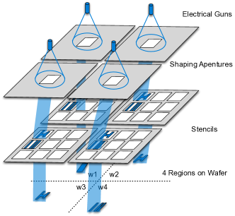
Even with decades of development, the key limitation of the EBL system has been and still is the low throughput. Recently, multi-column cell (MCC) system is proposed as an extension to CP technique [11, 12]. In MCC system, several independent character projections (CP) are used to further speed-up the writing process. Each CP is applied on one section of wafer, and all CPs can work parallelly to achieve better throughput. In morden MCC system, there are more than 1300 character projections (CPs) [13]. Since one CP is associated with one stencil, there are more than 1300 stencils in total. The manufacturing of stencil is similar to mask manufacturing. If each stencil is different, then the stencil preparation process would be very time consuming and expensive. Due to the design complexity and cost consideration, different CPs share one stencil design. One example of MCC printing process is illustrated in Fig. 1, where four CPs are bundled to generate an MCC system. In this example, the whole wafer is divided into four regions, and , and each region is printed through one CP. Note that the whole writing time of the MCC system is determined by the maximum one of the four regions. For modern design, because of the numerous distinct circuit patterns, only limited number of patterns can be employed on stencil. Since the area constraint of stencil is the bottleneck, the stencil should be carefully designed/manufactured to contain the most repeated cells or patterns.
Many previous works dealt with the design optimization for EBL system. [14, 15] considered EBL as a complementary lithography technique to print via/cut patterns. [16, 17] solved the subfield scheduling problem to reduce the critical dimension distortion. [18, 19, 20] proposed a set of layout/mask fracturing approaches to reduce the VSB shot number. Besides, several works solved the design challenges under CP technique. [21, 22] proposed several character design methods for both via layers and interconnect layers to achieve stencil area-efficiency.
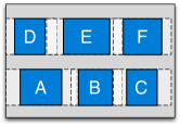
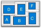
As one of the most challenges in CP mode, stencil planning has earned many attentions [23, 24, 25, 26, 27, 28]. When blank overlapping is not considered, the stencil planning equals to a character selection problem. [23] proposed an integer linear programming (ILP) formulation to select a group of characters for throughput maximization. When the characters can be overlapped to save more stencil space, the corresponding stencil planning is referred as overlapping-aware stencil planning (). [24, 25] investigated on problem to place more characters onto stencil. Recently, [26, 27] assumed that the pattern position in each character can be shifted, and integrated the character re-design into problem. As suggested in [24], the problem can be divided into two types: and . In , the standard cells with same height are selected into stencil. As shown in Fig. 2(a), each character implements one standard cell, and the enclosed circuit patterns of all the characters have the same height. Note that here we only show the horizontal blanks, and the vertical blanks are not represented because they are identical. In , the blank spaces of characters are non-uniform along both horizontal and vertical directions. By this way, stencil can contain both complex via patterns and regular wires. Fig. 2(b) illustrates a stencil design example for .
Compared with conventional EBL system, MCC system introduces two main challenges in problem. First, the objective is new: in MCC system the wafer is divided into several regions, and each region is written by one CP. Therefore the new should minimize the maximal writing times of all regions. However, in conventional EBL system the objective is simply minimize the wafer writing time. Besides, the stencil for an MCC system can contain more than 4000 characters, previous methodologies for EBL system may suffer from runtime penalty. However, no existing stencil planning work has been done toward the MCC system.
This paper presents E-BLOW, a comprehensive study to the MCC system and problems. Our main contributions are summarized as follows.
-
•
We provide the proof that both and problems are NP-hard.
-
•
We formulate integer linear programming (ILP) to co-optimizing characters selection and physical placements on stencil. To our best knowledge, this is the first mathematical formulation for both and .
-
•
We proposes a simplified formulation for .
-
•
We present a successive relaxation algorithm to find a near optimal solution.
-
•
We design a KD-Tree based clustering algorithm to speedup solution.
2 Preliminaries
In this section, we provide the preliminaries regarding overlapping aware stencil planning (). During character design, blank area is usually reserved around its boundaries. Note in this paper, the blank space refers to the blank around the character boundaries. The term “overlapping” means sharing blanks between adjacent characters. By this way, more characters can be placed on the stencil [24]. In this section, first we will provide the detailed problem formulation, then we will prove that both and are NP-hard.
2.1 Problem Formulation
In an MCC system with CPs, the whole wafer is divided into regions , and each region is written by one particular CP. We assume cell extraction [29] has been resolved first. In other words, a set of character candidates has already been given to the MCC system. For each character candidate , its writing time through VSB mode is denoted as , while its writing time through CP mode is .
The regions of wafer have different layout patterns, and the throughputs would be also different. Suppose character candidate repeats times on region . Let indicate the selection of character candidate as follows.
If is prepared on stencil, the total writing time of pattern on region is . Otherwise, should be printed through VSB. Since region comprises candidate , the writing time would be . Therefore, for region the total writing time is as follows:
where we denote , and . shows the writing time on when only VSB is applied, and represents the writing time reduction of candidate on region . In MCC system, for each region both and are constants. Therefore, the total writing time of the MCC system is formulated as follows:
| (1) |
Based on the notations above, we define the overlapping aware stencil planning () for MCC system as follows.
Problem 1.
OSP for MCC System: Given a set of character candidate , select a subset out of as characters, and place them on the stencil. The objective is to minimize the system writing time expressed by Eqn. (1), while the placement of is bounded by the outline of stencil. The width and height of stencil is and , respectively.
For convenience, we use the term to refer for MCC system in the rest of this paper.
2.2 NP-Hardness
In this subsection we will prove that both and are NP-hard. To facilitate the proof, we first define a Bounded Subset Sum () problem as follows.
Problem 2 (Bounded Subset Sum).
Given a list of numbers and a number , where , decide if there is a subset of the numbers that sums up to .
For example, given three numbers and , we can find a subset such that . Additionally, we can assumption that , where is some constant. Otherwise it be solved in time. Besides, without the bounded constraint , the problem becomes Subset sum problem, which is in NP-complete [30]. For simplicity of later explanation, let denote the set of numbers. Note that, we can assume that all the numbers are integer numbers.
Theorem 1.
problem is NP-complete.
The proof is in Appendix. In the following, we will show that even a simpler version of problem is NP-hard. In this simpler version, there is only one row in the stencil, and a set of characters is given. Besides, the blanks of each character are symmetric, and each character is with the same length .
Definition 1 (Minimum packing).
Given a subset of characters , its minimum packing is the packing with the minimum stencil length.
Lemma 1.
Given a set of character placed on a single row stencil. If for each character , both of its left and right blanks are , then the minimum packing is with the following stencil length
| (2) |
Proof.
Without loss of generality, we assume that . We prove by recursion that in an minimum length packing, the overlapping blank is . If there are only two characters, it is trivial that . We assume that when , the maximum overlapping blank . For the last character , the maximum sharing blank value is . Since for any , , we can simply insert it at either the left end or the right end, and find the incremental overlapping blank . Thus . Because the maximum overlapping blank for all characters is , we can see the minimum packing length is as in Eqn. (2). ∎
Lemma 2.
.
Proof.
Given an instance of with and , we construct a instance as follows:
-
•
The stencil length is set to , where .
-
•
For each , in there is a character , whose width is and both left and right blanks are . Since , the sum of left blank and right blank is less or equal to .
-
•
We introduce an additional character , whose width size is , and both left and right blanks are .
-
•
The VSB writing time of character is set to , while the VSB writing time for each character is set to . The CP writing times are set to 0 for all characters.
-
•
There is only one region, and each character repeats one time in the region.
For instance, given initial set and , the constructed instance is shown in Fig. 3.
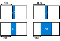
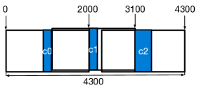
We will show the instance has a subset that adds up to if and only if the constructed instance has minimum packing length and total writing time smaller than .
( part) After solving the problem, a set of items are selected that they add up to . For each , character is also selected into the stencil. Besides, since the system writing time for is , it is trivial to see that in the instance the must be selected. Due to the Lemma 1, the minimum total packing length is
Meanwhile, the minimum total writing time in the is .
( part) We start from a instance with minimum packing length and total writing time smaller than , where a set of character are selected. Since the total total writing time must be smaller than , character . For all characters in set except , we select into the subset , which adds up to .
∎
Theorem 2.
is in NP-hard.
Theorem 3.
is in NP-hard.
3 E-BLOW for
When each character implements one standard cell, the enclosed circuit patterns of all the characters have the same height. The corresponding problem is called , which can be viewed as a combination of character selection and single row ordering problems [24]. Different from two-step heuristic proposed in [24], we show that these two problems can be solved simultaneously through a unified ILP formulation (3). For convenience, Table I lists the notations used in problem.
| width constraint of stencil or row | |
|---|---|
| number of characters | |
| number of rows | |
| x-position of character | |
| width of character | |
| horizontal overlap between and | |
| 0-1 variable, if is left of | |
| 0-1 variable, if is on th row |
In formulation (3), is the stencil width, is the number of rows. For each character , and are the width and the x-position, respectively. If and only if is assigned to -th row, . Otherwise, . Constraints (3) (3) are used to check position relationship between and . Here and , where is the overlapping when candidates and are packed together. Only when , i.e. both character and character are assigned to row , one of the two constraints (3) (3) will be active. Besides, for any three characters being assigned to row , i.e., , the and are self-consistent. That is, if is on the left of () and is on the left of (), then should be on the left of (). Similarly, if is on the right of () and is on the right of (), then should be on the right of () as well.
Since ILP is a well known NP-hard problem, directly solving it may suffer from long runtime penalty. One straightforward speedup method is to relax the ILP into the corresponding linear programming (LP) through replacing constraints (3) by the following:
It is obvious that the LP solution provides a lower bound to the ILP solution. However, we observe that the solution of relaxed LP could be like this: for each , and all the are assigned . Although the objective function is minimized and all the constraints are satisfied, this LP relaxation provides no useful information to guide future rounding, i.e., all the character candidates are selected and no ordering relationship is determined.
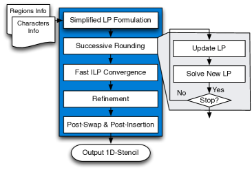
To overcome the limitation of above rounding, E-BLOW proposes a novel successive rounding framework to search near-optimal solution in reasonable runtime. As shown in Fig. 4, the overall flow includes several steps: Simplified ILP formulation, Successive Rounding, Fast ILP Convergence, Refinement, Post-swap and Post-Insertion. In section 3.1 the simplified formulation will be discussed, and its LP rounding lower bound will be proved. In section 3.2 the details of successive rounding would be introduced. In section 3.3 the Fast ILP convergence technique would be presented. In section 3.4 the refinement process is proposed. At last, to further improve the performance, in section 3.5 the post-swap and post-insertion techniques are discussed.
3.1 Simplified ILP Formulation
As discussed above, solving the ILP formulation (3) is very time consuming, and the related LP relaxation may be bad in performance. To overcome the limitations of (3), in this section we introduce a simplified ILP formulation, whose LP relaxation can provide good lower bound. The simplified formulation is based on a symmetrical blank (S-Blank) assumption: the blanks of each character are symmetric, i.e., left blank equals to right blank. is used to denote the blank of character . Note that for different characters and , their blanks and can be different.
At first glance the S-Blank assumption may lose optimality. However, it provides several practical and theoretical benefits. (1) In [24] the single row ordering problem was transferred into Hamilton Cycle problem, which is a well known NP-hard problem and even particular solver is quite expensive. In our work, instead of relying on expensive solver, under this assumption the problem can be optimally solved in . (2) Under S-Blank assumption, the ILP formulation can be effectively simplified to provide a reasonable rounding bound theoretically. Compared with previous heuristic framework [24], the proved rounding bound provides a better guideline for a global view search. (3) To compensate the inaccuracy in the asymmetrical blank cases, E-BLOW provides a refinement (see section 3.4).
The simplified ILP formulation is shown in Eqn. (4).
In the objective function of Eqn. (4), each character is associated with one profit value . The value is to evaluate the overall system writing time improvement if character is selected. Through assigning each character with one profit value, we can simplify the complex constraint (3). More details regarding the profit value setting would be discussed in Section 3.2. Besides, due to Lemma 1, constraint (4) and constraint (4) are for row width calculation, where (4) is to linearize operation. Here can be viewed as the maximum blank space of all the characters on row . Constraint (4) implies each character can be assigned into at most one row. It’s easy to see that the number of variables is , where is the number of characters, and is the number of rows. Generally speaking, single character number is much larger than row number . Thus compared with basic ILP formulation (3), the variable number in (4) can be reduced dramatically.
In our implementation, we set to , where and are ’s left blank and right blank, respectively. Note that here the ceiling function is used to make sure that under the S-Blank assumption, each blank is still integral. Although this setting may loss some optimality, E-BLOW provides post-stage to compensate the inaccuracy through incremental character insertion.
Now we will show that the LP relaxation of (4) has reasonable lower bound. To explain this, let us first look at a similar formulation (5) as follows:
| max | (5) | ||||
| s.t. | (5) | ||||
where is the maximum horizontal blank length of every character, i.e. . Program (5) is a multiple knapsack problem [31]. A multiple knapsack is similar to a knapsack problem, with the difference that there are multiple knapsacks. In formulation (5), each can be rephrased as .
Lemma 3.
If each is the same, the multiple knapsack problem (5) can find a approximation algorithm using LP rounding method.
For brevity we omit the proof, detailed explanations can be found in [32]. When all are the same, formulation (5) can be approximated to a max-flow problem. In addition, if we denote as /, we can achieve the following Lemma:
Proof.
First we introduce a modified formulation to program (5), where each is set to min. In other words, in the modified formulation, each is the same. Let and be the optimal values of (5) and the modified formulation, respectively. Let be the corresponding LP rounding result in the modified formulation. According to Lemma 3, . Since , we can get . In summary, . ∎
3.2 Successive Rounding
In this subsection we propose a successive rounding algorithm to solve program (4) iteratively. Successive rounding uses a simple iterative scheme in which fractional variables are rounded one after the other until an integral solution is found [33]. The ILP formulation (4) becomes an LP if we relax the discrete constraint to a continuous constraint as: .
The details of successive rounding is shown in Algorithm 1. At first we set all as unsolved since none of them is assigned to rows. The LP is updated and solved iteratively. For each new LP solution, we search the maximal , and store in (line 6). Then we find all that is closest to the maximum value , i.e., . In our implementation, is set to 0.9. For each selected variables , we try to pack into row , and set as solved. Note that when one character is assigned to one row, all would be set as solved. Therefore, the variable number in updated LP formulation would continue to decrease. This procedure repeats until no appropriate can be found. One key step of Algorithm 1 is the update (line 3). For each character , we set its as follows:
| (6) |
where is current writing time of region , and max . Through applying the , the region with longer writing time would be considered more during the LP formulation. During successive rounding, if is not assigned to any row, would continue to be updated, so that the total writing time of the whole MCC system can be minimized.
3.3 Fast ILP Convergence
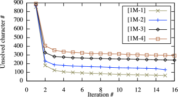
During successive rounding, for each LP iteration, we select some characters into rows, and set these characters as solved. In the next LP iteration, only unsolved characters would be considered in formulation. Thus the number of unsolved characters continues to decrease through the iterations. For four test cases (1M-1 to 1M-4), Fig. 5 illustrates the number of unsolved characters in each iteration. We observe that in early iterations, more characters would be assigned to rows. However, when the stencil is almost full, fewer of could be close to . Thus, in late iterations only few characters would be assigned into stencil, and the successive rounding requires more iterations.
To overcome this limitation so that the successive rounding iteration number can be reduced, we present a convergence technique based on fast ILP formulation. The basic idea is that when we observe only few characters are assigned into rows in one LP iteration, we stop successive rounding in advance, and call fast ILP convergence to assign all left characters. Note that in [25] an ILP formulation with similar idea was also applied. The details of the ILP convergence is shown in Algorithm 2. The input are the solutions of last LP rounding, and two parameters and . First we check each (lines 1-9). If , then we assume character would be not assigned to row , and set as solved. Similarly, if , we assign to row and set as solved. For those unsolved we build up ILP formulation (4) to assign final rows (lines 10-13).

At first glance the ILP formulation may be expensive to solve. However, we observe that in our convergence Algorithm 2, typically the variable number is small. Fig. 6 illustrates the solution distribution in last LP formulation. We can see that most of the values are close to 0. In our implementation and are set to 0.1 and 0.9, respectively. For this case, although the LP formulation contains more than 2500 variables, our fast ILP formulation results in only 101 binary variables.
3.4 Refinement
Refinement is a stage to solve the single row ordering problem [24], which adjusts the relative locations of input characters to minimize the total width. Under the S-Blank assumption, because of Lemma 1, this problem can be optimally solved through the following two-step greedy approach.
-
1.
All characters are sorted decreasingly by blanks;
-
2.
All characters are inserted one by one. Each one can be inserted at either left end or right end.


One example of the greedy approach is illustrated in Fig. 7, where four character candidates , , and are to be ordered. In Fig. 7(a), they are sorted decreasingly by blank space. Then all the candidates are inserted one by one. From the second candidate, each insertion has two options: left side or right side of the whole packed candidates. For example, if is inserted at the right of , has two insertion options: one is at the right side of (Fig. 7(b)), another is at the left side of (Fig. 7(d)). Given different choices of candidate , Fig. 7(c) and Fig. 7(e) give corresponding final solutions. Since from the second candidate each one has two choices, by this greedy approach candidates will generate possible solutions.
For the asymmetrical cases, the optimality does not hold anymore. To compensate the losing, E-BLOW consists of a refinement stage. For characters {}, single row ordering can have possible solutions. We avoid enumerating such huge solutions, and take advantage of the order in symmetrical blank assumption. That is, we pick up one best solution from the possible ones. Noted that although considering instead of options cannot guarantee optimal single row packing, our preliminary results show that the solution quality loss is negligible in practice.
The refinement is based on dynamic programming, and the details are shown in Algorithm 3. Refine(k) generates all possible order solutions for the first characters {}. Each order solution is represented as a set , where is the total length of the order, is the left blank of the left character, is the right blank of the right character, and is the character order. At the beginning, an empty solution set is initialized (line 1). If , then an initial solution would be generated (line 2). Here , and are width of first character , left blank of , and right blank of . If , then Refine(k) will recursively call Refine(k-1) to generate all old partial solutions. All these partial solutions will be updated by adding candidate (lines 5-9).
We propose pruning techniques to speed-up the dynamic programming process. Let us introduce the concept of inferior solutions. For any two solutions and , we say is inferior to if and only if , and . Those inferior solutions would be pruned during pruning section (lines 10-12). In our implementation, the is set to 20.
3.5 Post-Swap and Post-Insertion
After refinement, a post-swap stage is applied to further improve the performance. In each swap operation, an unselected character would be swapped with a character on stencil, if such swap can improve the writing time. The post-swap is implemented using a greedy flavor that consists of two steps. First, all the unselected characters are sorted. Second, the unselected characters would try to swap with the characters on stencils one by one.
After post-swap, a post-insertion stage is applied to further insert more characters into stencil. Different from the greedy insertion approach in [24] that new characters can be only inserted into one row’s right end. We consider to insert characters into the middle part of rows. Generally speaking, the character with higher profit value (6) would have a higher priority to be inserted into rows. We propose a character insertion algorithm to insert some additional characters into the rows. The insertion is formulated as a maximum weighted matching problem [34], under the constraint that for each row there is at most one character can be inserted. Although this assumption may loss some optimality, in practical it works quite well as usually the remaining space for a row is very limited.
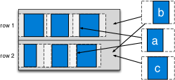

Fig. 8 illustrates one example of the character insertion. As shown in Fig. 8 (a), there are two rows (row 1, row 2) and three additional characters (). Characters and can be inserted into either row 1 or row 2, but character can only be inserted into row 2. It shall be noted that the insertion position is labeled by arrows. For example, two arrows from character mean that can be inserted into the middle of each row. We build up a bipartite graph to represent the relationships among characters and rows (see Fig. 8 (b)). Each edge is associated with a cost as character’s profit. By utilizing the bipartite graph, the best character insertion can be solved by finding a maximum weighted matching.
Given additional characters, we search the possible insertion positions under each row. The time complexity of searching all the possibilities is , where is the total row number and is the maximum character number on each row. We propose two heuristics to speed-up the search process. First, to reduce , we only consider those additional characters with high profits. Second, to reduce , we skip those rows with very little empty space.
4 E-BLOW for
Now we consider a more general case: the blank spaces of characters are non-uniform along both horizontal and vertical directions. This problem is referred to problem. In [24] the problem was transformed into a floorplanning problem. However, several key differences between traditional floorplanning and were ignored. (1) In there is no wirelength to be considered, while at floorplanning wirelength is a major optimization objective. (2) Compared with complex IP cores, lots of characters may have similar sizes. (3) Traditional floorplanner could not handle the problem size of modern MCC design.
4.1 ILP Formulation
| width (height) constraint of stencil | |
|---|---|
| width (height) of candidate | |
| horizontal (vertical) overlap between and | |
| , | |
| 0-1 variable, if is on stencil |
Here we will show that can be formulated as integer linear programming (ILP) as well. Compared with , is more general: the blank spaces of characters are non-uniform along both horizontal and vertical directions. The problem can be also formulated as an ILP formulation (7). For convenience, Table II lists some notations used in the ILP formulation. The formulation is motivated by [35], but the difference is that our formulation can optimize both placement constraints and character selection, simultaneously.
| min | (7) | ||||
| s.t. | (7) | ||||
| (7) | |||||
| (7) | |||||
| (7) | |||||
| (7) | |||||
| (7) | |||||
| (7) | |||||
where indicates whether candidate is on the stencil, and represent the location relationships between and . The number of variables is , where is number of characters. We can see that if , constraints (7) - (7) are not active. Besides, it is easy to see that when , for each of the four possible choices of , only one of the four inequalities (7) - (7) are active. For example, with () = (1,1,1,1), only the constraint (7) applies, which allows character to be anywhere above character . The other three constraints (7)-(7) are always satisfied for any permitted values of () and ().
Program (7) can be relaxed to linear programming (LP) by replacing constraint (7) as:
However, similar to the discussion in , the relaxed LP solution provides no information or guideline to the packing, i.e., every is set as , and every is set as . In other words, this LP relaxation provides no useful information to guide future rounding: all the character candidates are selected and no ordering relationship is determined. Therefore we can see that LP rounding method cannot be effectively applied to program (7).
4.2 Clustering based Simulated Annealing
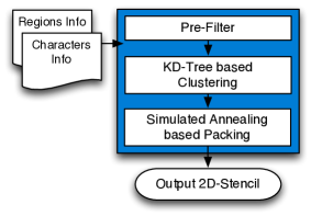
To deal with all these limitations of ILP formulation, an fast packing framework is proposed (see Fig. 9). Given the input character candidates, the pre-filter process is first applied to remove characters with bad profit (defined in (6)). Then the second step is a clustering algorithm to effectively speed-up the design process. Followed by the final floorplanner to pack all candidates.
Clustering is a well studied problem, and there are many of works and applications in VLSI [36] However, previous methodologies cannot be directly applied here. First, traditional clustering is based on netlist, which provides the all clustering options. Generally speaking, netlist is sparse, but in the connection relationships are so complex that any two characters can be clustered, and totally there are clustering options. Second, given two candidates and , there are several clustering options. For example, horizontal clustering and vertical clustering may have different overlapping blank space.
The main ideas of our clustering are iteratively search and group each character pair () with similar blank spaces, profits, and sizes. Character is said to be similar to , if the following condition is satisfied:
| (8) |
where and are the width and height of . and are the horizontal blank space and vertical blank space of , respectively. In our implementation, is set as 0.2. We can see that in clustering, all the size, blanks, and profits are considered.
The details of our clustering procedure are shown in Algorithm 4. First all the initial character candidates are sorted by (line 2), so those characters with more shot number reduction are tend to be clustered. Then all characters are labeled as unclustered (line 3). The clustering (lines 3-10) is repeated until no characters can be further merged. When cluster , the information of is modified to incorporate , and the is labeled as clustered.
For each candidate , finding available may need , and complexity of the horizontal clustering and vertical clustering are both . Then the complexity of the whole procedure is , where is the number of candidates.
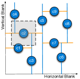
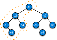
A KD-Tree [37] is used to speed-up the process of finding available pair . It provides fast region searching operations which keeping the time for insertion and deletion small: insertion, ; deletion of the root, ; deletion of a random node, . Using KD-Tree, the complexity of the Algorithm 4 can be reduced to . For instance, given nine character candidates {} as in Fig. 10 (a), the corresponding KD-Tree is shown in Fig. 10 (b). Note that KD-Tree can store multiple dimensional vertices, thus a single tree is enough to store all the information regarding width, height, blank spaces, and profits. For the sake of convenience, here characters are distributed only based on horizontal and vertical blank spaces. Thus only two dimensional space is illustrated in Fig. 10 (a). To search candidates with similar blank space with (see the shaded region of Fig. 10 (a)), it may need time to scan all candidates, where is the total candidate number. However, under the KD-Tree structure, this search procedure can be resolved in . All candidates scanned () are illustrated in Fig. 10 (b). Particularly, after scanning the , since is out of the search range, we can make sure the whole sub-tree rooted by is out of the search range as well.
In [24], the is transformed into a fixed-outline floorplanning problem. If a character candidate is outside the fixed-outline, then the character would not be prepared on stencil. Otherwise, the character candidate would be selected and packed on stencil. Parquet [38] was adopted as simulated annealing engine, and Sequence Pair [39] was used as a topology representation. In E-BLOW we apply a simulated annealing based framework similar to that in [24]. To demonstrate the effectiveness of our pre-filter and clustering methodologies, E-BLOW uses the same parameters.
5 Experimental Results
| char | CP | Greedy in [24] | [24] | [25] | E-BLOW | |||||||||
| # | # | T | char# | CPU(s) | T | char# | CPU(s) | T | char# | CPU(s) | T | char# | CPU(s) | |
| 1D-1 | 1000 | 1 | 64891 | 912 | 0.1 | 50809 | 926 | 13.5 | 19095 | 940 | 0.005 | 19479 | 940 | 2.1 |
| 1D-2 | 1000 | 1 | 99381 | 884 | 0.1 | 93465 | 854 | 11.8 | 35295 | 864 | 0.005 | 34974 | 866 | 1.7 |
| 1D-3 | 1000 | 1 | 165480 | 748 | 0.1 | 152376 | 749 | 9.13 | 69301 | 757 | 0.005 | 67209 | 766 | 1.7 |
| 1D-4 | 1000 | 1 | 193881 | 691 | 0.1 | 193494 | 687 | 7.7 | 92523 | 703 | 0.005 | 93816 | 703 | 4.5 |
| 1M-1 | 1000 | 10 | 63811 | 912 | 0.1 | 53333 | 926 | 13.5 | 39026 | 938 | 0.01 | 37848 | 944 | 3.8 |
| 1M-2 | 1000 | 10 | 104877 | 884 | 0.1 | 95963 | 854 | 11.8 | 77997 | 864 | 0.01 | 75303 | 874 | 3.5 |
| 1M-3 | 1000 | 10 | 172834 | 748 | 0.1 | 156700 | 749 | 9.2 | 138256 | 758 | 0.56 | 132773 | 774 | 9.3 |
| 1M-4 | 1000 | 10 | 200498 | 691 | 0.1 | 196686 | 687 | 7.7 | 176228 | 698 | 0.36 | 173193 | 711 | 7.4 |
| 1M-5 | 4000 | 10 | 274992 | 3604 | 1.0 | 255208 | 3629 | 1477.3 | 204114 | 3660 | 0.03 | 202401 | 3680 | 37.9 |
| 1M-6 | 4000 | 10 | 437088 | 3341 | 1.0 | 417456 | 3346 | 1182 | 357829 | 3382 | 0.03 | 348007 | 3420 | 48.4 |
| 1M-7 | 4000 | 10 | 650419 | 3000 | 1.0 | 644288 | 2986 | 876 | 568339 | 3016 | 0.59 | 563054 | 3064 | 54.0 |
| 1M-8 | 4000 | 10 | 820013 | 2756 | 1.0 | 809721 | 2734 | 730.7 | 731483 | 2760 | 0.42 | 721149 | 2818 | 54.7 |
| Avg. | - | - | 270680.4 | 1597.6 | 0.4 | 259958.3 | 1594.0 | 362.5 | 209123.8 | 1611.7 | 0.17 | 205767.2 | 1630.7 | 16.6 |
| Ratio | - | - | 1.32 | 0.98 | 0.02 | 1.26 | 0.98 | 19.01 | 1.02 | 0.99 | 0.01 | 1.0 | 1.0 | 1.0 |
E-BLOW is implemented in C++ programming language and executed on a Linux machine with two 3.0GHz CPU and 32GB Memory. GUROBI [40] is used to solve ILP/LP. The benchmark suite from [24] are tested (1D-1, , 1D-4, 2D-1, , 2D-4). To evaluate the algorithms for MCC system, eight benchmarks (1M-x) are generated for and the other eight (2M-x) are generated for the problem. In these new benchmarks, character projection (CP) number are all set to 10. For each small case (1M-1, , 1M-4, 2M-1, , 2M-4) the character candidate number is 1000, and the stencil size is set to . For each larger case (1M-5 , , 1M-8, 2M-5, , 2M-8) the character candidate number is 4000, and the stencil size is set to . The size and the blank width of each character are similar to those in [24]. It shall be noted that [24] is aimed for single CP system, for MCC system it is modified to optimize the total writing time of all the regions.
5.1 Comparison for
For , Table III compares E-BLOW with the greedy method in [24], the heuristic framework in [24], and the algorithms in [25]. We have obtained the programs of [24] and executed them in our machine. The results of [25] are directly from their paper. Column “char #” is number of character candidates, and column “CP#” is number of character projections. For each algorithm, we report “T”, “char#” and “CPU(s)”, where “T” is the writing time of the E-Beam system, “char#” is the character number on final stencil, and “CPU(s)” reports the runtime. From Table III we can see E-BLOW achieves better performance than both greedy method and heuristic method in [24]. Compared with E-BLOW, the greedy method has more system writing time, while [24] introduces more system writing time. One possible reason is that different from the greedy/heuristic methods, E-BLOW proposes mathematical formulations to provide global view. Additionally, due to the successive rounding scheme, E-BLOW is around 22 faster than the work in [24].
E-BLOW is further compared with one recent solver [25] in Table III. E-BLOW found stencil placements with best E-Beam system writing time for 10 out of 12 test cases. In addition, for all the MCC system cases (1M-1, , 1M-8) E-BLOW outperforms [25]. One possible reason is that to optimize the overall throughput of the MCC system, a global view is necessary to balance the throughputs among different regions. E-BLOW utilizes the mathematical formulations to provide such global optimization. Although the linear programming solvers are more expensive than the deterministic heuristics in [25], the runtime of E-BLOW is reasonable that each case can be finished in 20 seconds on average.
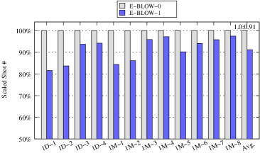
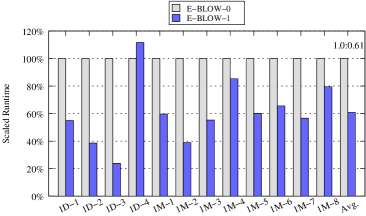
We further demonstrate the effectiveness of the fast ILP convergence (Section 3.3) and post-insertion (Section 3.5). We denote E-BLOW-0 as E-BLOW without these two techniques, and denote E-BLOW-1 as E-BLOW with these techniques. Fig. 11 and Fig. 12 compare E-BLOW-0 and E-BLOW-1, in terms of system writing time and runtime, respectively. From Fig. 11 we can see that applying fast ILP convergence and post-insertion can effectively E-Beam system throughput, that is, averagely 9% system writing time reduction can be achieved. In addition, Fig. 12 demonstrates the performance of the fast ILP convergence (see Section 3.3). We can see that in 11 out of 12 test cases, the fast ILP convergence can effectively reduce E-BLOW CPU time. The possible reason for the slow down in case 1D-4 is that when fast convergence is called, if there are still many unsolved variables, ILP solver may suffer from runtime overhead problem. However, if more successive rounding iterations are applied before ILP convergence, less runtime can be reported.
| char | CP | Greedy in [24] | [24] | E-BLOW | |||||||
| # | # | T | char # | CPU(s) | T | char # | CPU(s) | T | char # | CPU(s) | |
| 2D-1 | 1000 | 1 | 159654 | 734 | 2.1 | 107876 | 826 | 329.6 | 105723 | 789 | 65.5 |
| 2D-2 | 1000 | 1 | 269940 | 576 | 2.4 | 166524 | 741 | 278.1 | 170934 | 657 | 52.5 |
| 2D-3 | 1000 | 1 | 290068 | 551 | 2.6 | 210496 | 686 | 296.7 | 178777 | 663 | 56.4 |
| 2D-4 | 1000 | 1 | 327890 | 499 | 2.7 | 240971 | 632 | 301.7 | 179981 | 605 | 54.7 |
| 2M-1 | 1000 | 1 | 168279 | 734 | 2.1 | 122017 | 811 | 313.7 | 91193 | 777 | 58.6 |
| 2M-2 | 1000 | 1 | 283702 | 576 | 2.4 | 187235 | 728 | 286.1 | 163327 | 661 | 48.7 |
| 2M-3 | 1000 | 1 | 298813 | 551 | 2.6 | 235788 | 653 | 289.0 | 162648 | 659 | 52.3 |
| 2M-4 | 1000 | 1 | 338610 | 499 | 2.7 | 270384 | 605 | 285.6 | 195469 | 590 | 53.3 |
| 2M-5 | 4000 | 10 | 824060 | 2704 | 19.0 | 700414 | 2913 | 3891.0 | 687287 | 2853 | 59.0 |
| 2M-6 | 4000 | 10 | 1044161 | 2388 | 20.2 | 898530 | 2624 | 4245.0 | 717236 | 2721 | 60.7 |
| 2M-7 | 4000 | 10 | 1264748 | 2101 | 21.9 | 1064789 | 2410 | 3925.5 | 921867 | 2409 | 57.1 |
| 2M-8 | 4000 | 10 | 1331457 | 2011 | 22.8 | 1176700 | 2259 | 4550.0 | 1104724 | 2119 | 57.7 |
| Avg. | - | - | 550115 | 1218.1 | 8.3 | 448477 | 1324 | 1582.7 | 389930.5 | 1291.9 | 56.375 |
| Ratio | - | - | 1.41 | 0.94 | 0.15 | 1.15 | 1.02 | 28.1 | 1.0 | 1.0 | 1.0 |
5.2 Comparison for
For , Table IV gives the similar comparison. For each algorithm, we also record “T”, “char #” and “CPU(s)”, where the meanings are the same with that in Table III. Compared with E-BLOW, although the greedy algorithm is faster, its design results would introduce 41% more system writing time. Furthermore, compared with E-BLOW, although the framework in [24] puts 2% characters onto stencil, it gets 15% more system writing time. The possible reason is that in E-BLOW the characters with similar writing time are clustered together. The clustering method can help to speed-up the packaging, so E-BLOW is faster than [24]. In addition, after clustering the character number can be reduced. With smaller solution space, the simulated annealing engine is easier to achieve a better solution, in terms of system writing time.
From both tables we can see that compared with [24], E-BLOW can achieve a better tradeoff between runtime and system throughput.
| candidate# | ILP | E-BLOW | ||||||
| binary# | T | char# | CPU(s) | T | char# | CPU(s) | ||
| 1T-1 | 8 | 64 | 434 | 6 | 0.5 | 434 | 6 | 0.1 |
| 1T-2 | 10 | 100 | 1034 | 6 | 26.1 | 1034 | 6 | 0.2 |
| 1T-3 | 11 | 121 | 1222 | 6 | 58.3 | 1222 | 6 | 0.2 |
| 1T-4 | 12 | 144 | 1862 | 6 | 1510.4 | 1862 | 6 | 0.2 |
| 1T-5 | 14 | 196 | NA | NA | 3600 | 2758 | 6 | 0.1 |
| 2T-1 | 6 | 66 | 60 | 6 | 37.3 | 207 | 5 | 0.1 |
| 2T-2 | 8 | 120 | 354 | 6 | 40.2 | 653 | 7 | 0.1 |
| 2T-3 | 10 | 190 | 1050 | 6 | 436.8 | 4057 | 4 | 0.1 |
| 2T-4 | 12 | 276 | NA | NA | 3600 | 4208 | 5 | 0.2 |
5.3 E-BLOW vs. ILP
We further compare the E-BLOW with the ILP formulations (3) and (7). Although for both problems the ILP formulations can find optimal solutions theoretically, they may suffer from runtime overhead. Therefore, we randomly generate nine small benchmarks, five for (“1T-x”) and four for (“2T-x”). The sizes of all the character candidates are set to . For benchmarks, the row number is set to 1, and the row length is set to 200. The comparisons are listed in Table V, where column “candidate#” is the number of character candidates. “ILP” and “E-BLOW” represent the ILP formulation and our E-BLOW framework, respectively. In ILP formulation, column “binary#” gives the binary variable number. For each mode, we report “T”, “char#” and “CPU(s)”, where “T” is E-Beam system writing time, “char#” is character number on final stencil, and “CPU(s)” is the runtime. Note that in Table V the ILP solutions are optimal.
Let us compare E-BLOW with ILP formulation for 1D cases (1T-1, , 1T-5). E-BLOW can achieve the same results with ILP formulations, meanwhile it is very fast that all cases can be finished in 0.2 seconds. Although ILP formulation can achieve optimal results, it is very slow that a case with 14 character candidates (1T-5) can not be solved in one hour. Next, let us compare E-BLOW with ILP formulation for 2D cases (2T-1, , 2T-4). For 2D cases ILP formulations are slow that if the character candidate number is 12, it cannot finish in one hour. E-BLOW is fast, but with some solution quality penalty.
Although the integral variable number for each case is not huge, we find that in the ILP formulations, the solutions of corresponding LP relations are vague. Therefore, expensive search method may cause unacceptable runtimes. From these cases ILP formulations are impossible to be directly applied in problem, as in MCC system character number may be as large as .
6 Conclusion
In this paper, we have proposed E-BLOW, a tool to solve OSP problem in MCC system. For , a successive relaxation algorithm and a dynamic programming based refinement are proposed. For , a KD-Tree based clustering method is integrated into simulated annealing framework. Experimental results show that compared with previous works, E-BLOW can achieve better performance in terms of shot number and runtime, for both MCC system and traditional EBL system. Note that the extra cost for multiple stencils is mostly the cost of multiple stencil design, thus different regions tend to have specific stencils to improve the throughput. However, if a shared stencil is well-designed and optimized that such sharing can achieve very comparable throughput, we can even reduce the stencil design cost. In that situation, sharing stencil design could be attractive, especially for the companies that have limited design budget. As EBL, including MCC system, are widely used for mask making and also gaining momentum for direct wafer writing, we believe a lot more research can be done for not only stencil planning, but also EBL aware design.
Acknowledgment
This work is supported in part by NSF grants CCF-0644316 and CCF-1218906, SRC task 2414.001, NSFC grant 61128010, and IBM Scholarship. The authors would like to thank Prof. Shiyan Hu at Michigan Technological University and Zhao Song at University of Texas for helpful comments.
References
- [1] A. B. Kahng, C.-H. Park, X. Xu, and H. Yao, “Layout decomposition for double patterning lithography,” in IEEE/ACM International Conference on Computer-Aided Design (ICCAD), 2008, pp. 465–472.
- [2] H. Zhang, Y. Du, M. D. Wong, and R. Topaloglu, “Self-aligned double patterning decomposition for overlay minimization and hot spot detection,” in IEEE/ACM Design Automation Conference (DAC), 2011, pp. 71–76.
- [3] B. Yu, K. Yuan, B. Zhang, D. Ding, and D. Z. Pan, “Layout decomposition for triple patterning lithography,” in IEEE/ACM International Conference on Computer-Aided Design (ICCAD), 2011, pp. 1–8.
- [4] B. Yu and D. Z. Pan, “Layout decomposition for quadruple patterning lithography and beyond,” in IEEE/ACM Design Automation Conference (DAC), 2014, pp. 1–6.
- [5] D. Z. Pan, B. Yu, and J.-R. Gao, “Design for manufacturing with emerging nanolithography,” IEEE Transactions on Computer-Aided Design of Integrated Circuits and Systems (TCAD), vol. 32, no. 10, pp. 1453–1472, 2013.
- [6] Y. Arisawa, H. Aoyama, T. Uno, and T. Tanaka, “EUV flare correction for the half-pitch 22nm node,” in Proceedings of SPIE, vol. 7636, 2010.
- [7] L.-W. Chang, X. Bao, B. Chris, and H.-S. Philip Wong, “Experimental demonstration of aperiodic patterns of directed self-assembly by block copolymer lithography for random logic circuit layout,” in IEEE International Electron Devices Meeting (IEDM), 2010.
- [8] H. C. Pfeiffer, “New prospects for electron beams as tools for semiconductor lithography,” in Proceedings of SPIE, vol. 7378, 2009.
- [9] A. Fujimura, “Design for E-Beam: design insights for direct-write maskless lithography,” in Proceedings of SPIE, vol. 7823, 2010.
- [10] T. Maruyama, M. Takakuwa, Y. Kojima, Y. Takahashi, K. Yamada, J. Kon, M. Miyajima, A. Shimizu, Y. Machida, H. Hoshino, H. Takita, S. Sugatani, and H. Tsuchikawa, “EBDW technology for EB shuttle at 65nm node and beyond,” in Proceedings of SPIE, vol. 6921, 2008.
- [11] H. Yasuda, T. Haraguchi, and A. Yamada, “A proposal for an MCC (multi-column cell with lotus root lens) system to be used as a mask-making e-beam tool,” in Proceedings of SPIE, vol. 5567, 2004.
- [12] T. Maruyama, Y. Machida, S. Sugatani, H. Takita, H. Hoshino, T. Hino, M. Ito, A. Yamada, T. Iizuka, S. Komatsue, M. Ikeda, and K. Asada, “CP element based design for 14nm node EBDW high volume manufacturing,” in Proceedings of SPIE, vol. 8323, 2012.
- [13] M. Shoji, T. Inoue, and M. Yamabe, “Extraction and utilization of the repeating patterns for CP writing in mask making,” in Proceedings of SPIE, vol. 7748, 2010.
- [14] J.-R. Gao, B. Yu, and D. Z. Pan, “Self-aligned double patterning layout decomposition with complementary e-beam lithography,” in IEEE/ACM Asia and South Pacific Design Automation Conference (ASPDAC), Jan 2014, pp. 143–148.
- [15] Y. Du, H. Zhang, M. D. Wong, and K.-Y. Chao, “Hybrid lithography optimization with e-beam and immersion processes for 16nm 1D gridded design,” in IEEE/ACM Asia and South Pacific Design Automation Conference (ASPDAC), 2012, pp. 707–712.
- [16] S. Babin, A. B. Kahng, I. I. Mandoiu, and S. Muddu, “Resist heating dependence on subfield scheduling in 50kV electron beam maskmaking,” in Proceedings of SPIE, vol. 5130, 2003.
- [17] S.-Y. Fang, W.-Y. Chen, and Y.-W. Chang, “Graph-based subfield scheduling for electron-beam photomask fabrication,” IEEE Transactions on Computer-Aided Design of Integrated Circuits and Systems (TCAD), vol. 32, no. 2, pp. 189–201, 2013.
- [18] A. B. Kahng, X. Xu, and A. Zelikovsky, “Fast yield-driven fracture for variable shaped-beam mask writing,” in Proceedings of SPIE, vol. 6283, 2006.
- [19] X. Ma, S. Jiang, and A. Zakhor, “A cost-driven fracture heuristics to minimize sliver length,” in Proceedings of SPIE, vol. 7973, 2011.
- [20] B. Yu, J.-R. Gao, and D. Z. Pan, “L-Shape based layout fracturing for E-Beam lithography,” in IEEE/ACM Asia and South Pacific Design Automation Conference (ASPDAC), 2013, pp. 249–254.
- [21] P. Du, W. Zhao, S.-H. Weng, C.-K. Cheng, and R. Graham, “Character design and stamp algorithms for character projection electron-beam lithography,” in IEEE/ACM Asia and South Pacific Design Automation Conference (ASPDAC), 2012, pp. 725–730.
- [22] R. Ikeno, T. Maruyama, T. Iizuka, S. Komatsu, M. Ikeda, and K. Asada, “High-throughput electron beam direct writing of VIA layers by character projection using character sets based on one-dimensional VIA arrays with area-efficient stencil design.” in IEEE/ACM Asia and South Pacific Design Automation Conference (ASPDAC), 2013, pp. 255–260.
- [23] M. Sugihara, T. Takata, K. Nakamura, R. Inanami, H. Hayashi, K. Kishimoto, T. Hasebe, Y. Kawano, Y. Matsunaga, K. Murakami, and K. Okumura, “Cell library development methodology for throughput enhancement of character projection equipment,” IEICE Transactions on Electronics, vol. E89-C, pp. 377–383, 2006.
- [24] K. Yuan, B. Yu, and D. Z. Pan, “E-Beam lithography stencil planning and optimization with overlapped characters,” IEEE Transactions on Computer-Aided Design of Integrated Circuits and Systems (TCAD), vol. 31, no. 2, pp. 167–179, Feb. 2012.
- [25] J. Kuang and E. F. Young, “A highly-efficient row-structure stencil planning approach for E-Beam lithography with overlapped characters,” in ACM International Symposium on Physical Design (ISPD), 2014.
- [26] C. Chu and W.-K. Mak, “Flexible packed stencil design with multiple shaping apertures for e-beam lithography,” in IEEE/ACM Asia and South Pacific Design Automation Conference (ASPDAC), 2014, pp. 137–142.
- [27] W.-K. Mak and C. Chu, “E-Beam lithography character and stencil co-optimization,” IEEE Transactions on Computer-Aided Design of Integrated Circuits and Systems (TCAD), vol. 33, 2014.
- [28] D. Guo, Y. Du, and M. D. Wong, “Polynomial time optimal algorithm for stencil row planning in E-Beam lithography,” in IEEE/ACM Asia and South Pacific Design Automation Conference (ASPDAC), 2015.
- [29] S. Manakli, H. Komami, M. Takizawa, T.Mitsuhashi, and L. Pain, “Cell projection use in mask-less lithography for 45nm & 32nm logic nodes,” in Proceedings of SPIE, vol. 7271, 2009.
- [30] S. Arora and B. Barak, Computational Complexity: A Modern Approach. Cambridge University Press, 2009.
- [31] S. Martello and P. Toth, Knapsack Problems: Algorithms and Computer Implementations. John Wiley & Sons, Inc., 1990.
- [32] M. Dawande, J. Kalagnanam, P. Keskinocak, F. Salman, and R. Ravi, “Approximation algorithms for the multiple knapsack problem with assignment restrictions,” Journal of Combinatorial Optimization, vol. 4, pp. 171–186, 2000.
- [33] E. L. Johnson, G. L. Nemhauser, and M. W. Savelsbergh, “Progress in linear programming-based algorithms for integer programming: An exposition,” INFORMS Journal on Computing, vol. 12, no. 1, pp. 2–23, 2000.
- [34] Z. Galil, “Efficient algorithms for finding maximum matching in graphs,” ACM Computing Surveys, vol. 18, no. 1, pp. 23–38, Mar. 1986.
- [35] S. Sutanthavibul, E. Shragowitz, and J. Rosen, “An analytical approach to floorplan design and optimization,” IEEE Transactions on Computer-Aided Design of Integrated Circuits and Systems (TCAD), vol. 10, no. 6, pp. 761–769, jun 1991.
- [36] C. J. Alpert and A. B. Kahng, “Recent directions in netlist partitioning: a survey,” Integration, the VLSI Journal, vol. 19, pp. 1–81, August 1995.
- [37] J. L. Bentley, “Multidimensional binary search trees used for associative searching,” Communications of the ACM, vol. 18, pp. 509–517, September 1975.
- [38] S. N. Adya and I. L. Markov, “Fixed-outline floorplanning: Enabling hierarchical design,” IEEE Transactions on Very Large Scale Integration Systems (TVLSI), vol. 11, no. 6, pp. 1120–1135, 2003.
- [39] H. Murata, K. Fujiyoshi, S. Nakatake, and Y. Kajitani, “VLSI module placement based on rectangle-packing by the sequence-pair,” IEEE Transactions on Computer-Aided Design of Integrated Circuits and Systems (TCAD), vol. 12, pp. 1518–1524, 1996.
- [40] Gurobi Optimization Inc., “Gurobi optimizer reference manual,” http://www.gurobi.com, 2014.
PROOF OF THEOREM 1
Lemma 5.
problem is in NP.
Proof.
It is easy to see that problem is in NP. Given a subset of integer numbers , we can add them up and verify that their sum is in polynomial time. ∎
Lemma 6.
.
Proof.
In problem, we are given clauses over variables . Besides, there are three literals in each clause, which is the OR of some number of literals. Eqn. (9) gives one example of , where and .
| (9) |
Without loss of generality, we can have the following assumptions:
-
1.
No clause contains both variable and . Otherwise, any such clause is always true and we can just eliminate them from the formula.
-
2.
Each variable appears in at least one clause. Otherwise, we can just assign any arbitrary value to the variable .
To convert a instance to a instance, we create two integer numbers in set for each variable and three integer numbers in for each clause . All the numbers in set and are in base 10. Besides, , so that the bounded constraints are satisfied. All the details regarding and are defined as follows.
-
•
In the set , all integer numbers are with digits, and the first digit are always 1.
-
•
In the set , we construct two integer numbers and for the variable . For both of the values, the digits after the first ‘1’ serve to indicate the corresponding variable in . That is, the digit in these digits is set to 1 and all others are 0. For the next digits, the digit is set to 1 if the clause contains the respective literal. The last digits are always 0.
-
•
In the set , we also construct three integer numbers and for each clause . In where , the first digits after the first ‘1’ are 0, and in the next digits all are 0 except the index setting to . The last digits are all 0 except the index setting to 1.
-
•
, where is an integer number with digits. The first digits of are 1, in the next digits all are 4, and in the last digits all are 1.
Based on the above rules, given the instance in Eqn. (9) the constructed set and target are shown in Fig. 13. Note that the highest digit achievable is 9, meaning that no digit will carry over and interfere with other digits.
| = | 1 | 1 | 0 | 0 | 0 | 1 | 0 | 0 | 0 | |
|---|---|---|---|---|---|---|---|---|---|---|
| = | 1 | 1 | 0 | 0 | 0 | 0 | 1 | 0 | 0 | |
| = | 1 | 0 | 1 | 0 | 0 | 0 | 1 | 0 | 0 | |
| = | 1 | 0 | 1 | 0 | 0 | 0 | 0 | 0 | 0 | |
| = | 1 | 0 | 0 | 1 | 0 | 0 | 0 | 0 | 0 | |
| = | 1 | 0 | 0 | 1 | 0 | 1 | 0 | 0 | 0 | |
| = | 1 | 0 | 0 | 0 | 1 | 0 | 0 | 0 | 0 | |
| = | 1 | 0 | 0 | 0 | 1 | 1 | 1 | 0 | 0 | |
| = | 1 | 0 | 0 | 0 | 0 | 1 | 0 | 1 | 0 | |
| = | 1 | 0 | 0 | 0 | 0 | 2 | 0 | 1 | 0 | |
| = | 1 | 0 | 0 | 0 | 0 | 3 | 0 | 1 | 0 | |
| = | 1 | 0 | 0 | 0 | 0 | 0 | 1 | 0 | 1 | |
| = | 1 | 0 | 0 | 0 | 0 | 0 | 2 | 0 | 1 | |
| = | 1 | 0 | 0 | 0 | 0 | 0 | 3 | 0 | 1 | |
| = | 6 | 1 | 1 | 1 | 1 | 4 | 4 | 1 | 1 | |
| = | 1 | 1 | 1 | 1 | 4 | 4 | 1 | 1 |
Claim 1.
The instance has a satisfying truth assignment iff the constructed instance has a subset that adds up to .
Proof of part of Claim: If the instance has a satisfying assignment, we can pick a subset containing all for which is set to true and for which is set to false. We should then be able to achieve by picking the necessary to get 4’s in the . Due to the last ‘1’ in , for each only one would be selected from . Besides, we can see totally numbers would be selected from .
Proof of part of Claim: If there is a subset that adds up to , we will show that it corresponds to a satisfying assignment in the instance. must include exactly one of and , otherwise the th digit value of cannot be satisfied. If , in the we set to true; otherwise we set it to false. Similarly, must include exactly one of and , otherwise the last digits of cannot be satisfied. Therefore, all clauses in the are satisfied and has a satisfying assignment.
∎
For instance, given a satisfying assignment of Eqn. (9): , the corresponding subset is . We set , where , and then . We can see that .