Bicep2 III: Instrumental Systematics

Abstract

In a companion paper, we have reported a $>5\sigma$ detection of degree scale $B$-mode polarization at 150 GHz by the Bicep2 experiment. Here we provide a detailed study of potential instrumental systematic contamination to that measurement. We focus extensively on spurious polarization that can potentially arise from beam imperfections. We present a heuristic classification of beam imperfections according to their symmetries and uniformities, and discuss how resulting contamination adds or cancels in maps that combine observations made at multiple orientations of the telescope about its boresight axis. We introduce a technique, which we call “deprojection,” for filtering the leading order beam-induced contamination from time-ordered data, and show that it reduces power in Bicep2’s actual and null-test $BB$ spectra consistent with predictions using high signal-to-noise beam shape measurements. We detail the simulation pipeline that we use to directly simulate instrumental systematics and the calibration data used as input to that pipeline. Finally, we present the constraints on $BB$ contamination from individual sources of potential systematics. We find that systematics contribute $BB$ power that is a factor $\sim 10\times$ below Bicep2’s three-year statistical uncertainty, and negligible compared to the observed $BB$ signal. The contribution to the best-fit tensor/scalar ratio is at a level equivalent to $r=(3-6)\times 10^{-3}$.

1. Introduction

Since the the discovery of the $2.7$ K cosmic microwave background (CMB) by Penzias & Wilson (1965), rapid progress in instrumental sensitivity has permitted the detection of progressively subtler effects. The $\sim 100~{}\mu$K temperature anisotropies, measured to high precision by the WMAP and Planck satellites (Hinshaw et al., 2013; Planck Collaboration et al., 2014c) and by ground-based telescopes (Sievers et al., 2013; Story et al., 2013; Das et al., 2014; Hou et al., 2014), are $\sim 10^{-5}$ fluctuations in the 2.7 K background. The degree scale primary CMB temperature anisotropies are polarized at the $\sim 1\%$ level (Kovac et al., 2002), with fluctuations of the order of $1~{}\mu$K. This polarization, which arises as a natural consequence of the same acoustic oscillations that source the temperature anisotropies (Bond & Efstathiou, 1984), is curl-free ($E$-mode) and its angular power spectrum is uniquely predicted given the temperature ($T$) spectrum with the addition of no additional cosmological parameters. The agreement of the $E$-mode spectrum with the predictions given the best fitting $T$ spectrum is a striking, independent confirmation of $\Lambda$CDM, modern cosmology’s basic paradigm (Pryke et al., 2009; QUIET Collaboration et al., 2012; Barkats et al., 2014; Crites et al., 2014; Naess et al., 2014).

Fainter still is the divergence-free ($B$-mode) polarization of the CMB that would be caused by gravitational waves present in the Universe at the time of recombination (Polnarev, 1985; Kamionkowski et al., 1997; Seljak, 1997; Seljak & Zaldarriaga, 1997). Because the production of a stochastic background of gravitational waves is a generic prediction of inflationary models (Grishchuk, 1975; Starobinsky, 1979; Rubakov et al., 1982; Fabbri & Pollock, 1983; Abbott & Wise, 1984), the detection of the cosmological $B$-mode polarization would constitute direct evidence for an era of cosmic inflation. The amplitude of the cosmological $B$-mode spectrum is parametrized by the tensor/scalar ratio $r$. An $r=0.1$ $B$-mode signal has degree scale fluctuations of the order of $100~{}$nK, a factor $10$ smaller than the $E$-mode anisotropy, a factor $10^{3}$ smaller than the unpolarized anisotropy, and a factor $10^{8}$ smaller than the CMB monopole.

Measuring CMB polarization anisotropy is made difficult by its weakness relative to the unpolarized anisotropy and by the additional sources of systematic error specific to polarization measurements. Effects that convert CMB temperature anisotropy into a false polarization signal are of particular importance. This is especially true for $B$-mode measurements because both the temperature and the expected inflationary $B$-mode spectra peak at similar angular scales. Detecting and characterizing a $B$-mode polarization signal of this magnitude requires controlling systematics to a level to match the experiment’s unprecedentedly low instrumental noise.

In Bicep2 Collaboration I (2014), hereafter the Results Paper, we present a detection of $B$-mode power in $>5\sigma$ excess over the lensed-$\Lambda$CDM CMB expectation. In this paper, we present extensive studies of possible systematic contamination in this measurement using detailed calibration data that allow us to directly predict or place stringent upper limits on it. We find that systematics contribute power at a level subdominant to Bicep2’s statistical noise and negligible compared to the measured $B$-mode spectrum.

The structure of this paper is as follows. In Section 2 we briefly review the aspects of the Bicep2 instrument that are most important for an understanding of potential systematic contamination. In Section 3 we review the noise estimation procedure and show that our debiased auto spectrum procedure is equivalent to a cross spectral analysis. In Section 4 we review how Bicep2’s specific observing strategy modulates the contamination from beam systematics in the signal maps and in our internal consistency checks. In Section 5 we introduce the deprojection algorithm we use to mitigate contamination from beam imperfections. In Section 6 we review external beam shape measurements. In Section 7 we detail the simulation pipeline used to predict the level of spurious polarization due to imperfect beam shapes. In Section 8 we review Bicep2’s “jackknife” internal consistency null tests and discuss the classes of systematics to which each is sensitive. In Section 9 we check that deprojection of CMB data does indeed recover the known beam non-idealities within uncertainties, even in the presence of realistic template noise. In Section 10 we present the constraints on many potential sources of systematic contamination. We conclude in Section 11. In a series of four appendices we provide the formal definition of our elliptical Gaussian beam parametrization (Appendix A), an expanded discussion of beam shape mismatch (Appendix B), the mathematical and practical details of deprojection (Appendix C), and a discussion of the uncertainties in the beam mismatch simulations (Appendix D).

2. Instrument design and observational strategy

The Bicep2 instrument is discussed in depth in Bicep2 Collaboration II (2014), hereafter the Instrument Paper. Here we highlight the details most relevant to systematics, and in particular those that can cause false polarization. In this section we describe how effects can arise in the antennas (beam shape and pointing), in the bolometers (thermal mismatch), or in the readout (crosstalk). We also describe several aspects of the observing strategy that serve to suppress these systematics and/or to aid in identifying them.

2.1. Instrument Design

Each camera “pixel” in Bicep2’s focal plane consists of two orthogonally polarized beam-forming antennas (O’Brient et al., 2012; Bicep2 Collaboration et al., 2015) that couple incoming radiation to two bolometric detectors (each antenna is coupled to its own detector). We label the members of an antenna/detector pair (which we refer to simply as a “detector pair”) “A” and “B.” The A and B antennas within a pair are spatially coincident in the focal plane so they nominally observe the same location on the sky. The time-ordered data, or “timestreams,” from the A and B detectors are summed to measure the total intensity of the incoming radiation and differenced to measure its polarized component. Therefore, any mechanism other than the intrinsic polarization of the sky signal that produces a differential signal in the A and B detectors will produce spurious polarization if not properly accounted for.

The response of an antenna to incoming radiation as a function of angle is called its beam. One class of systematics that can cause a false polarization is a difference in the beam shape or beam center (“centroid’) of the A and B detectors. Beam shape imperfections or centroid offsets that are common to A and B do not cause a false polarization. We observe that Bicep2’s beams exhibit significant systematic centroid mismatch within a pair, which we call “differential pointing,” and which we have precisely characterized.

In the time-reversed sense, each antenna illuminates the telescope aperture with a nearly Gaussian pattern (Kuo et al., 2008). The illumination pattern (i.e. the “near-field beam”) is truncated on a $26.4$ cm cold aperture stop. The asymmetric truncation of the near-field beams will induce an expected far-field beam asymmetry. We observe an expected dependence of detectors’ beam ellipticity on the radial position in the focal plane. Because we treat beam shapes and centroids fully empirically, a precise understanding of the mechanisms governing them is not required for assessing systematic contamination. A brief review of the parametrization and measurements of Bicep2’s beams is given in Section 5.1 and Section 6, respectively. A fully detailed treatment is given in Bicep2 and Keck Array Collaborations IV (2015), hereafter the Beams Paper.

We have designed the telescope shielding system and our observation strategy to mitigate contamination from the ground and the Galaxy. A co-moving forebaffle and fixed ground shield ensure that at the lowest observing elevation rays originating from the ground must diffract twice before entering the telescope aperture. The brightest parts of the Galaxy are always well outside of the angle intersected by the co-moving forebaffle. The lowest galactic latitude of the observations is $b=-39^{\circ}$, and we have measured that for a typical detector $<0.1\%$ of the total integrated power is found outside of $25^{\circ}$ from the main beam with the co-moving forebaffle installed. Details are in the Beams Paper.

Bicep2’s bolometers are transition edge sensors (TESs). We measure the amount of incident radiation by tracking, as a function of time, the amount of electrical power (presumed to be in addition to the radiative power) required to maintain the TES at a fixed point in the superconducting/normal transition. Thermal drifts in the focal plane thus produce spurious signals in the detector timestreams. A false polarization signal arises if the responses of the A and B bolometers to these thermal fluctuations are different. We mitigate thermal drift using a combination of passive thermal filters and active thermal control (Kaufman, 2014). We then continuously measure any remaining thermal fluctuations to high precision using neutron transmutation doped (NTD) germanium thermistors located on the focal plane, allowing us to directly constrain spurious signal from thermal drift (see Section 10.8).

The bolometers are read out using multiplexed superconducting quantum interference devices (SQUIDs) (Irwin et al., 2002). The use of SQUID readouts introduces susceptibility to pickup from magnetic fields. Bicep2 employs a combination of high magnetic permeability and superconducting shielding to block external magnetic fields, and its scan strategy allows for nearly perfect filtering (“ground subtraction”) of pickup that is constant in time and a function of telescope pointing direction, as is expected of most magnetic fields. The multiplexing of detector timestreams (de Korte et al., 2003) creates crosstalk between channels in the cryogenic and room temperature readout hardware. Crosstalk, which we have measured in a variety of ways, can also produce false polarization.

Using calibration data we make detailed calculations of the impact of the above effects in Section 10 below.

2.2. Observational Strategy and Data Cuts

The Bicep2 telescope was situated on an azimuth/elevation mount that performed constant elevation scans at a fixed azimuth center. The scans spanned just over $60^{\circ}$ in azimuth and were re-centered on a new azimuth at approximately one hour intervals, during which time the sky moved in azimuth by $15^{\circ}$. Because the sky changed position with respect to the scan boundaries, we can differentiate between signals that are scan synchronous (ground-fixed signal), and signals that rotate with the sky. By subtracting the mean of all scans from each scan we exactly remove any contaminating signal that is a function of scan position and is constant over hour-long timescales. We refer to this filtering as “ground subtraction.” This method was used successfully by Bicep1 (Chiang et al., 2010; Barkats et al., 2014) and by the QUIET experiment (QUIET Collaboration et al., 2012).

The Bicep2 mount also allowed for a third axis of motion, the rotation of the entire telescope about the boresight. Bicep2 observed at four distinct boresight orientations, or “deck angles”: $68^{\circ}$, $113^{\circ}$, $248^{\circ}$, and $293^{\circ}$. (At $0^{\circ}$, the rows of Bicep2’s focal plane were roughly perpendicular to the horizon.) Because Bicep2’s detector polarization angles were all aligned in the focal plane, reconstructing maps of Stokes $Q$ and $U$ requires a minimum of two deck angles, optimally separated by $45^{\circ}$, $135^{\circ}$, or $225^{\circ}$. A valid deck angle pair cannot be separated by $180^{\circ}$. With Bicep2’s four deck angles, a map formed from one valid deck angle pair (e.g. $68^{\circ}$ and $113^{\circ}$) is complementary to the map made from the other deck angle pair (e.g. $248^{\circ}$ and $293^{\circ}$). The deck angle pair that is complementary to any of the four valid pairs is rotated $180^{\circ}$ from it.

We guard against systematics arising from unusually functioning detectors by removing them during map making. The map making process uses data from only a subset of the nominally functioning (i.e. optically responsive) detectors. We implement a series of channel cuts that exclude detector pairs having certain properties outside a pre-defined range. The details are discussed in Section  13.7 of the Instrument Paper. When we have a priori reason to believe that a systematic will contaminate a few detectors much more strongly than others, we can also perform a detector pair exclusion test in which we remake maps cutting the most contamination-prone pairs. For the test to be considered passed, we require that the change in the resulting maps and power spectra is consistent with the corresponding changes in systematics-free simulations.

2.3. Summary

We address systematics using a combination of five general strategies. Three strategies reduce contamination in the final maps.

1. Natural mitigation: Bicep2’s maps are built up from observations made with many detectors. A systematic that varies between detector pairs will thus statistically average down in the final map. Bicep2’s maps are also built from observations at four deck angles. Some systematics cancel with instrument rotation. This is discussed further in Section 4.

2. Time-domain filtering: We remove atmospheric $1/f$ noise by applying a third-order polynomial filter to the timestreams. Atmospheric noise is not a systematic because it averages down over time and is accounted for in the noise model, but such a filter also removes any large angular scale contamination that might not average down. In addition, we also exactly remove any remaining signal that is fixed with respect to the ground or scan (as opposed to the sky) by applying the ground subtraction filter discussed in Section 2.2.

3. Deprojection: We also filter out the map modes most contaminated by beam imperfections. If they are ignored, differences in beam shape between the two detectors of a detector pair will transform bright temperature anisotropies into false polarization anisotropies. We have developed a technique to explicitly filter the handful of map modes contaminated by several major types of beam mismatch, and to account for this removal in power spectrum estimation. This technique is described in Section 5 and in Appendices A-D.

Two strategies characterize the level of contamination remaining in the maps.

1. Jackknife maps: Many classes of systematics produce different contamination in different subsets of data. As part of our internal consistency checks, we split Bicep2’s data set into two halves, form $Q$ and $U$ maps from each of the halves, difference these maps, and test whether the resulting residuals are consistent with the difference of systematics-free, signal-plus-noise simulations. We refer to these null tests as “jackknives,” and they are discussed in more detail in Section 8. We refer to the un-differenced maps, made with the full data set, from which the science analysis in the Results Paper derives, as the “signal” maps. We refer to the angular power spectra of those maps as the signal spectra.

2. Time-domain simulations: Our analysis pipeline generates simulated realizations of time-ordered data (signal and noise) for each detector, which is then processed in exactly the same manner as our real data. We have extended our pipeline to optionally incorporate the effects of various instrumental systematics into these simulated data, which allows us to model their effects on the final power spectra and $r$ estimate. This pipeline is described in Section 7, with particular regard given to simulating beam mismatch effects. Measurements of beam mismatch are presented in Section 6. The results of these studies are presented in Section 10.

Generally speaking, time-domain simulations allow us to model the consequences of known systematic effects. Jackknife maps are useful for empirically constraining contamination from both known and unknown systematics.

3. Noise estimation

The Results Paper describes the construction of “noise pseudosimulations” that we use to estimate the noise bias and uncertainty of our measured auto spectrum. We construct these pseudosimulations by differencing the two maps made from two halves of a random permutation of $17,000$ temporal subsets of the full data set, which are long enough (approximately 1h each) to have minimal noise correlations. We impose a constraint that each half have the same total weight. Jackknife noise pseudosimulations are similarly constructed by randomly permuting the subsets within a jackknife half and differencing the two maps in each half separately. As described in the Results Paper, this noise estimation procedure has been checked against two alternative techniques and all are found to yield equivalent results.

More formally, the $j$th random permutation splits the full data set to define two half maps $M_{1j},M_{2j}$, which can be recombined by summing or differencing:

$$M = {\textstyle\frac{1}{2}}(M_{1j}+M_{2j})$$

$$N_{j} = {\textstyle\frac{1}{2}}(M_{1j}-M_{2j}).$$ (1)

$M$ is our standard full map and is the same for any split, while $N_{j}$ is the noise realization. The auto spectra of these two maps can be written

$$M\!\!\times\!\!M = {\textstyle\frac{1}{4}}[M_{1j}\!\!\times\!\!M_{1j}+2(M_{1j}\!\!\times\!\!M_{2j})+M_{2j}\!\!\times\!\!M_{2j}]$$ (2)

$$N_{j}\!\!\times\!\!N_{j} = {\textstyle\frac{1}{4}}[M_{1j}\!\!\times\!\!M_{1j}-2(M_{1j}\!\!\times\!\!M_{2j})+M_{2j}\!\!\times\!\!M_{2j}].$$ (3)

Subtracting these gives

$$M\!\!\times\!\!M-N_{j}\!\!\times\!\!N_{j}=M_{1j}\!\!\times\!\!M_{2j}.$$ (4)

We see that subtracting the auto spectrum of a single noise pseudosimulation $N_{j}$ from that of the full map is identical to taking the cross-spectrum of the two corresponding half maps.

Our actual noise bias and uncertainty estimation uses an ensemble of $N\sim 500$ noise pseudosimulations. We noise debias the auto spectrum of the full map by subtracting the mean of the auto spectra of the noise realizations,

$$M\!\!\times\!\!M-\left<N_{j}\!\!\times\!\!N_{j}\right>=\left<M\!\!\times\!\!M-N_{j}\!\!\times\!\!N_{j}\right>=\left<M_{1j}\!\!\times\!\!M_{2j}\right>.$$ (5)

where brackets represent mean over the $j=1...N$ realizations of the ensemble. This shows that our debiasing procedure is equivalent to computing the mean of cross-spectra between data subsets for a large number of splits. Similarly, the higher order statistics (variance, skewness, etc.) of the noise pseudosimulations are mathematically equivalent to the higher order statistics of the cross-spectra formed between the data subsets. One can go on to demonstrate that our procedure is also equivalent to taking the mean of cross-spectra between many smaller data split chunks (Fowler et al., 2010; Lueker et al., 2010; Story et al., 2013). As in any such cross-spectrum analysis, in the limit of uncorrelated noise between data subsets, there can be no residual noise bias from incorrect noise modeling, as our “noise model” is in fact not a model, but rather a linear combination of the data themselves.

The main effect that could possibly correlate noise among data subsets is anisotropic turbulent structure in the atmosphere. The spatial structure of the turbulence above the telescope averages down over time but persists on timescales of the order or the height of the turbulent layer divided by the wind speed at that altitude. (The timescale only becomes shorter if the turbulent structure is not assumed to be “frozen in” in the frame of the moving atmosphere but instead also evolves in time.) For a height of $5$ km and a wind speed of $5$ m s^-1, the timescale is $\sim 15$ minutes. The data subsets we use are approximately $1$ hr in duration, so even in the unpolarized pair sum timestreams, the noise properties of which are dominated by turbulent atmospheric emission, we expect very little noise correlation between data subsets. Furthermore, because the atmosphere is almost totally unpolarized, pair-differencing of detector pairs almost completely eliminates the noise due to atmospheric turbulence, leaving only the white noise of random photon arrival times. The cancellation of unpolarized atmospheric turbulent emission is apparent in Figure 22 of the Instrument Paper, which shows that the instantaneous temporal power spectrum of the unfiltered pair-difference timestreams is dominated by white noise, with a possible contribution from atmospheric turbulence at most a few percent at the lowest frequencies.

Lastly, any remaining polarization noise correlations are further suppressed by the time-domain filtering described in Section 2.3, which downweights the lowest frequency Fourier modes along the scan direction. These are the modes with the highest fractional contribution of atmospheric turbulence to the total noise.

4. Beam systematics in maps

Table 1Transformation of beam mismatch leakage under rotation

Rotation	Monopole (e.g. Diff. Gain, Beamwidth)	Dipole (e.g. Centroid Offset)	Quadrupole (e.g. Diff. Ellipticity)
$45^{\circ}$	$E\rightarrow B$, $B\rightarrow E$	$E\rightarrow(E+E^{\prime})/\sqrt{2}$, $B\rightarrow(B+B^{\prime})/\sqrt{2}$	$E\rightarrow E$, $B\rightarrow B$
$90^{\circ}$	$E\rightarrow-E$, $B\rightarrow-B$	$E\rightarrow E^{\prime}$, $B\rightarrow B^{\prime}$	$E\rightarrow E$, $B\rightarrow B$
$180^{\circ}$	$E\rightarrow E$, $B\rightarrow B$	$E\rightarrow-E$, $B\rightarrow-B$	$E\rightarrow E$, $B\rightarrow B$

Note. — In a map formed by a detector pair at one set of projected orientations on the sky, this table summarizes how the spurious signal from beam mismatch of the given symmetry is transformed in a second map made from the same detector pair at a second set of orientations rotated from the first by the given angle.

We refer to any differential response to incoming unpolarized radiation between the A and B members of a detector pair as “beam mismatch.” In the presence of beam mismatch, the pair-difference signal will, in general, be non-zero even when observing an unpolarized source. This signal directly enters polarization maps and so must be filtered out or otherwise accounted for. One can think of such potential contamination as the unpolarized temperature field “leaking” into the pair-difference signal of a given detector pair. We refer to this as temperature-to-polarization (T$\rightarrow$P) leakage. At high galactic latitude at $150$ GHz, CMB $T$ is much brighter than foregrounds and is the dominant unpolarized signal sourcing T$\rightarrow$P leakage.

The leaked signal, $d$, that enters the pair-difference data of a given detector pair is the convolution of the unpolarized sky with the difference of the pair’s A and B beams,

$$d_{T\rightarrow P} = T(\mathbf{\hat{n}})\ast\left[B_{A}(\mathbf{\hat{n}})-B_{B}(\mathbf{\hat{n}})\right]$$ (6)

$$\equiv T(\mathbf{\hat{n}})\ast B_{\delta}(\mathbf{\hat{n}})$$

where $T$ is the unpolarized temperature field, $B$ is the response of a detector, and $\mathbf{\hat{n}}$ is the sky coordinate. If the difference beam, $B_{\delta}$, is non-axially symmetric, then $d_{T\rightarrow P}$ is a function of both the pointing direction of the detector pair and the projected orientation of $B_{\delta}$ on the sky.

Given measurements of $T(\mathbf{\hat{n}})$ and $B_{\delta}(\mathbf{\hat{n}})$, Equation 6 is sufficient to predict the instantaneous T$\rightarrow$P leakage in a detector pair’s pair-difference timestream as a function of that pair’s pointing direction. Predicting how this timestream level contamination manifests in polarization maps requires knowledge of the observing strategy. In principle, timestream level simulations of beam mismatch that go all the way to final maps capture the map level contamination without the need for any heuristic understanding. Nonetheless, to gain confidence that these simulations accurately reflect reality, it is helpful to build intuition about the way in which different classes of beam mismatch interact with the observing strategy to produce the map level contamination. The remainder of this section attempts to develop this intuition.

We treat each detector pair’s difference beam as the linear combination of different components, or modes,

$$B_{\delta}(\mathbf{\hat{n}})=\sum_{k}a_{k}B_{\delta k}(\mathbf{\hat{n}})$$ (7)

Our map making procedure is a linear process. Thus, the contamination in the final maps is a linear combination of the contamination produced by each of these modes individually. How each mode contaminates the final map depends upon its amplitude $a_{k}$, its coherence across detector pairs in the focal plane, and its symmetry under rotation of the instrument with respect to the sky. Amplitude sets the magnitude of the systematic in time-ordered data, while coherence and symmetry determine the degree of cancellation in maps made from multiple detectors and at multiple deck angles.

4.1. Incoherence Across the Focal Plane

When combining data from multiple detector pairs to form a map, the T$\rightarrow$P leakage from a difference beam mode that randomly varies among detector pairs will average down if $\left<a_{k}\right>=0$, where the expectation value of the $k$th mode is over detector pairs. Since any map pixel is only sampled by a finite number of detectors, the averaging down is only partial. Nonetheless, because the contamination in maps made from different subsets of detector pairs will be different, the jackknife tests described in Section 8 that check for consistency between detector pairs will fail. In general, jackknife maps have the same noise level as the signal maps. Because a randomly varying beam systematic will contaminate the signal map as much as a pair selection jackknife, we expect pair selection jackknives to fail when the contamination in the signal map is comparable to Bicep2’s statistical uncertainty.

More worrisome are beam systematics that are correlated between detector pairs, the leakage from which does not necessarily average down and can potentially evade jackknives. Bicep2’s many pair selection jackknives test for consistency between subsets of detectors whose beam mismatch is expected to be different for various mechanisms, e.g. varying by position in the focal plane or by multiplex column.

4.2. Symmetry

A difference beam mode that is common to all detector pairs (i.e. fully coherent across the focal plane) will not produce any contamination of pair selection jackknives and will not average down when combining data from detector pairs. However, under an azimuthal rotation of the beam about its center, the leakage from modes of certain symmetries will change sign. When combining data from detectors at different projected orientations on the sky, the leakage from even fully coherent mismatch will sometimes nearly exactly cancel in the signal maps (O’Dea et al., 2007; Shimon et al., 2008; QUIET Collaboration et al., 2011). Whether or not this occurs depends on the azimuthal symmetry of the mode. Bicep2 heavily exploits this cancellation effect by performing deck angle rotation. When this cancellation occurs in the signal maps, the contaminating signals in both halves of the corresponding deck angle jackknife map are equal to each other but opposite in sign, so that the jackknife experiences no such cancellation. In this case, the deck angle jackknife will fail for levels of contamination that are negligible in the signal map. Appropriate deck angle jackknifes are thus highly sensitive probes of T$\rightarrow$P leakage from these beam systematics.

In analogy with the azimuthal symmetry of pure monopoles, dipoles, and quadrupoles, we classify difference beam modes as having monopolar symmetry (i.e. invariant under rotation, i.e. azimuthally symmetric), dipolar symmetry (reversing sign under $180^{\circ}$ rotation), or quadrupolar symmetry (reversing sign under $90^{\circ}$ rotation); other symmetries are possible for complex beam shapes, but are not modeled here. Table 1 summarizes how $d_{T\rightarrow P}$ from these modes is reconstructed as a false polarization signal in a polarization map depending on the mode’s projected orientation on the sky. The reconstructed leakage from a monopole symmetric mode changes sign under a $90^{\circ}$ rotation. (Thus, leakage to $+E$ and $+B$ at one orientation leaks to $-E$ and $-B$ at the second; adding these two maps results in cancellation of the leakage, and subtracting them to form a jackknife multiplies the contamination by two.) The reconstructed leakage from a dipole symmetric mode changes sign under a $180^{\circ}$ rotation. The reconstructed leakage from a quadrupole symmetric mode is invariant under rotation.

In a given map pixel, the cancellation of T$\rightarrow$P leakage from a monopole or dipole symmetric mode will occur if that pixel is sampled at appropriate orientations by the same detector pair. If the pixel is sampled by different detector pairs, then it is only the leakage from the common component that cancels due to the rotation. Full cancellation of the T$\rightarrow$P leakage from the monopole or dipole symmetric modes thus requires that one of two corresponding criteria be met: either (1) the sky coverage of any given detector pair is the same at all deck angles, or (2) the contribution to any final map pixel is from detector pairs with identical $a_{k}$.

Boresight rotation, in addition to rotating a detector pair’s beam, also changes its pointing direction. Because the instantaneous field of view of Bicep2’s focal plane is large compared to the overall map boundaries, the area of sky mapped by a given detector is different at different deck angles. This is illustrated in Figure 1, which shows the map regions sampled by two detector pairs, one located near the center of the focal plane and one located near the edge. The coverage of the detector pair located near the center of the focal plane is largely the same at different deck angles; the coverage of the detector pair located near the edge of the focal plane is very different at different deck angles. As a consequence, detector pairs near the center of the focal plane (and thus the central regions of the signal maps) satisfy criterion (1) and experience highly efficient cancellation. Detector pairs near the edge of the focal plane still experience cancellation, but only in so far as they satisfy criterion (2).

The remainder of this section considers in more detail the cancellation of leakage from difference beams of different symmetries.

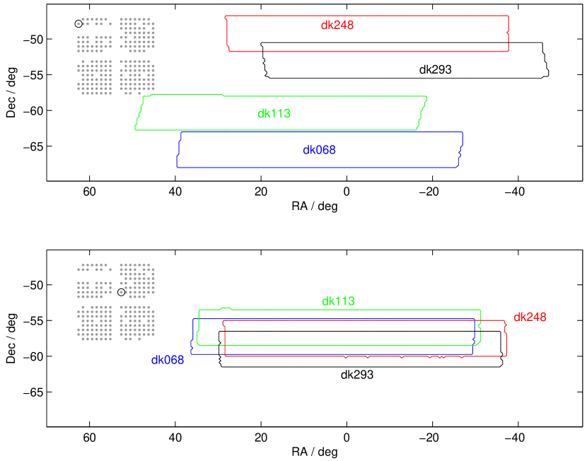
Figure 1.— Map coverage of a single Bicep2 detector pair located (top panel) near the edge of the focal plane and (bottom panel) near the center of the focal plane. The coverage at different deck angles overlaps significantly for central detectors but not at all for edge detectors. The inset (not drawn to scale) indicates the location of the detector pair in the focal plane.

Table 2Summary of Beam Mismatch Leakage Effects

Symmetry:	Monopole	Dipole	Quadrupole
Incoherent across focal plane
In signal map:	Averages down	Averages down	Averages down
In pair selection jackknife:	Potentially contaminates	Potentially contaminates	Potentially contaminates
Coherent across focal plane
In signal map:	Cancels under $90^{\circ}$ rot.	Cancels under $180^{\circ}$ rot.	Does not cancel
In deck angle jackknife:	Contaminates in $90^{\circ}$ jackknife	Contaminates in $180^{\circ}$ jackknife	Does not contaminate

Note. — In a map formed by many detector pairs at multiple projected focal plane orientations on the sky this table summarizes the behavior of T$\rightarrow$P beam systematics having various symmetries.

4.2.1 Monopole Symmetric Difference Beam

Examples of monopole symmetric difference beams are the difference of two circular Gaussians with different peak heights or widths, as illustrated in the upper and lower left panels of Figure 2. We focus on these particular modes because the calibration measurements presented in Section 6 indicate that they describe the majority of Bicep2’s monopole symmetric beam mismatch. However, we note that the discussion here is generally applicable to any monopole symmetric difference beam.

If $d_{T\rightarrow P}$ for a detector pair pointed at some location on the sky is from a monopole symmetric difference beam, it remains constant under rotation of the difference beam. However, because the polarization sensitivity of the pair (i.e. the interpretation of that signal under the assumption that it is not a systematic and “on the sky”) rotates as well, how $d_{T\rightarrow P}$ is reconstructed in the final map does change. If the leakage is reconstructed as a false polarization with some magnitude and direction at one orientation, rotating the detector pair $90^{\circ}$ causes it to be reconstructed as false polarization with equal magnitude but rotated $90^{\circ}$ from the first. Rotating a polarization vector by $90^{\circ}$ simply transforms $+Q\rightarrow-Q$ and $+U\rightarrow-U$, so combining the measurements cancels the T$\rightarrow$P leakage.

Bicep2’s scan strategy did not cancel leakage from monopole symmetric difference beams in this way. Bicep2’s observation strategy included only $180^{\circ}$ deck angle pair complements and no $90^{\circ}$ complements. In maps made from deck angle pairs separated by $180^{\circ}$, the T$\rightarrow$P leakage from monopole symmetric difference beams is reconstructed as $Q$ and $U$ identically. This leakage adds in the signal map and cancels in the deck jackknife, making the deck jackknives Bicep2 forms insensitive to this type of leakage.

Bicep2’s successor experiment, the Keck Array (Sheehy et al., 2010; Kernasovskiy et al., 2012), consists of five Bicep2-like receivers with common boresight pointing and oriented at $72^{\circ}$ increments to one another. This leads to an effective fivefold increase in the number of deck angles and thus a certain degree of cancellation of monopole symmetric beam mismatch in the final coadded map. Monopole symmetric mismatch that is common between the focal planes of the two experiments will thus be suppressed in cross-spectra taken between them. Beginning in 2013, the Keck Array added the additional four $90^{\circ}$ complementary deck angles necessary to fully cancel leakage from coherent monopole symmetric difference beams and to form deck jackknives that can test for it. Recently, Bicep2 and Keck Array Collaborations V (2015) demonstrated consistency between Bicep2 and Keck Array’s auto and cross spectra.

The predecessor experiment to Bicep2 was Bicep1 (Yoon et al., 2006). Bicep1 also observed at the same deck angle intervals as Bicep2, but because the polarization angles of Bicep1’s detector pairs were not uniformly oriented in the focal plane like Bicep2 and Keck Array’s, a monopole symmetric difference beam common to Bicep1 and Bicep2 will also be suppressed in a cross-spectrum.

In summary, even though monopole symmetric beam mismatch does not contaminate Bicep2’s deck jackknives, it will (1) contaminate the Keck Array’s $90^{\circ}$ deck angle jackknife, (2) contaminate Bicep1’s pair selection jackknives, and (3) not produce fully correlated power in cross-spectra formed between any of these experiments. Lastly, we expect the deprojection technique described in Section 5 to fully remove T$\rightarrow$P leakage from gain and beamwidth mismatch, both of which have monopole symmetric difference beams. We empirically test this last proposition via the beam map simulations described in Section 7.

4.2.2 Dipole Symmetric Difference Beam

An example of a difference beam having dipolar symmetry is the difference of two identical circular Gaussians with offset centroids, as illustrated in the top middle and right panels of Figure 2. As discussed in Section 6, this “differential pointing” is also Bicep2’s dominant source of T$\rightarrow$P leakage.

Dipole symmetric difference beam $d_{T\rightarrow P}$ changes sign under a $180^{\circ}$ rotation. Because the rotation of the detector polarization angles is also $180^{\circ}$, the reconstructed spurious polarization is equal in magnitude and opposite in sign. Again, averaging the maps cancels the leakage; subtracting the maps to form Bicep2’s deck jackknife boosts the contamination by a factor of two. Bicep2’s set of deck angles does include $180^{\circ}$ complements. The high degree of cancellation in the signal map relative to the deck jackknife makes the deck jackknife a powerful probe of dipole symmetric contamination. This is discussed in more detail in Section 9.

4.2.3 Quadrupole Symmetric Difference Beam

An example of a quadrupole symmetric difference beam is the difference of two elliptical Gaussians with mismatched magnitudes and/or directions of their elongations, and is illustrated in the bottom middle and right panels of Figure 2. In this case it is the difference between the pair polarization sensitivity angle and the orientation angle of the quadrupolar pattern which determines the nature of the leakage — $0^{\circ}$ and $90^{\circ}$ leak $T\rightarrow\pm E$ while $\pm 45^{\circ}$ leak $T\rightarrow\pm B$ (Shimon et al., 2008).

A quadrupole symmetric difference beam $d_{T\rightarrow P}$ changes sign under a $90^{\circ}$ rotation. This is the same periodicity as a real polarized sky signal, so no amount of boresight rotation can distinguish it from real polarization for a single pair. As explained in Section 4.1, leakage from incoherent beam mismatch with any symmetry averages down over pairs in the signal map and potentially contaminates pair selection jackknives. Coherent quadrupolar mismatch produces leakage that is indistinguishable from real sky polarization. No possible jackknife can test for this. For this reason, coherent quadrupole symmetric beam mismatch is especially pernicious and must be carefully controlled. In Section 10.1, we accurately simulate the real beam mismatch and correctly predict the effects of ellipticity mismatch in our data (this being the dominant quadrupole symmetric component).

4.3. Summary

Table 2 summarizes the situation. Any component of $B_{\delta}(\mathbf{\hat{n}})$ that varies randomly across the focal plane(s) averages down to at least some degree — even for quadrupolar effects so long as the orientations are random — and in general we expect residual contamination to be as strong in the jackknife maps as in the signal map. For a component of $B_{\delta}(\mathbf{\hat{n}})$ that is coherent across the focal plane(s), whether or not there is cancellation in the signal map under instrument rotation depends on the symmetry of the component, as does the jackknife split required to expose the systematic. A subtlety is the issue of whether each pair self-cancels under instrument rotation. This will be true in the limit that the focal plane field of view is small compared to the size of the map, and becomes less true as the field of view approaches the size of the map (as is the case for Bicep2).

5. Deprojection technique

As introduced in Section IV.F of the Results Paper, we have developed an analysis technique, which we call “deprojection,” to filter out T$\rightarrow$P leakage from beam mismatch (and potentially other effects). Such a filter renders our analysis immune to contamination from leading order beam imperfections. In this section, we describe the technique as we have implemented it for the Bicep2 analysis. Testing of the performance of the algorithm in our case is deferred to Section 9.

5.1. Beam Parametrization

We model $B_{\delta}(\mathbf{\hat{n}})$ as the difference of two elliptical Gaussians. In principle, we are free to choose any model with which to parametrize and mitigate T$\rightarrow$P leakage, but the elliptical Gaussian parametrization is convenient.

Six parameters define an elliptical Gaussian: one for peak height, two for the center of the ellipse (centroid), one for width, and two specifying ellipticity. The two parameters for ellipticity are often taken as a magnitude and orientation. We choose an alternate but equivalent basis — plus- and cross-ellipticity, denoted $p$ and $c$ — that describes an ellipse oriented either vertically/horizontally or at $\pm 45^{\circ}$ to the horizontal axis. The mathematical details of the parametrization are given in Appendix A.

We model intra-pair gain mismatch (differential gain) as a difference in Gaussian peak height; the difference beam mode for differential gain, $B_{\delta g}(\mathbf{\hat{n}})$, is therefore just a circular Gaussian. We model differential pointing as a centroid offset in an $x/y$ coordinate system fixed with respect to the focal plane and centered on the nominal beam center; the corresponding difference beam modes, $B_{\delta x}(\mathbf{\hat{n}})$ and $B_{\delta y}(\mathbf{\hat{n}})$, are the differences of circular Gaussians offset in either the $x$ or $y$ direction. (Bicep2’s beams are $\sim 0.5^{\circ}$ FWHM, so making the flat sky approximation and parametrizing the ellipse on a Cartesian coordinate system centered on each beam center is an adequate approximation.) Beamwidth mismatch is parametrized by a difference in Gaussian width $\sigma$. Differential plus- and cross-ellipticity are defined as the differences of purely plus-elliptical or purely cross-elliptical Gaussians whose orientations are defined with respect to the same focal plane fixed coordinate system in which differential pointing is described.

Figure 2 shows the differential elliptical Gaussian modes. We consider the total difference beam to be a linear combination of these modes in isolation, so that the sum in Equation 7 is over $k=\{g,x,y,\sigma,p,c\}$.

5.2. Algorithm

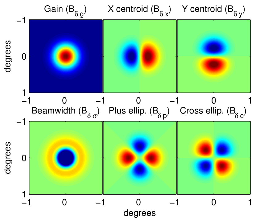
Figure 2.— Differences of elliptical Gaussian beams, which we choose for $B_{\delta k}(\mathbf{\hat{n}})$. The total difference beam, $B_{\delta}(\mathbf{\hat{n}})$, is a linear combination of these modes. Differential gain and beamwidth produce monopole symmetric difference beams, differential pointing a dipole symmetric difference beam, and differential ellipticity a quadrupole symmetric difference beam. These difference beams couple to different derivatives of the underlying CMB temperature field.

Because the T$\rightarrow$P leakage from beam mismatch is deterministic and beam shapes are constant in time, we can filter some of it out by constructing leakage templates corresponding to the differential modes of elliptical Gaussians, fitting them to our data, and subtracting them. Such a method prevents contamination arising from the component of Bicep2’s beams described by elliptical Gaussians from entering the maps. It requires no a priori knowledge of the actual magnitude of the mismatch (Aikin, 2013; Sheehy, 2013).

To second order, the individual modes of a differential elliptical Gaussian couple to distinct linear combinations of $T(\mathbf{\hat{n}})$ and its first and second derivatives (Hu et al., 2003). Appendix B provides a heuristic description of this coupling. Given maps of $T(\mathbf{\hat{n}})$ and its spatial derivatives (which we refer to as the “template maps”) and knowledge of the pointing of each of Bicep2’s detector pairs as a function of time (as required for map making), we sample the template maps along each detector pair’s pointing trajectory to create derivative timestreams. We use the chain rule for derivatives to express the derivatives with respect to the Bicep2 focal plane coordinate system as projected on the sky at each step in the time series. The derivative timestreams are given by

$$d_{i,j}(t)=\nabla^{i}_{j}\tilde{T}(t)$$ (8)

where the $i$th spatial derivative is defined with respect to the focal plane coordinate $j=\{x,y\}$,

$$\nabla^{i}_{j}\equiv\frac{\partial^{i}}{\partial j^{i}},$$ (9)

and the tilde denotes that the template map has been pre-convolved by a circular Gaussian beam of nominal width, $\sigma$.

We then form the linear combinations of $d_{i,j}(t)$ that correspond to leakage from differential elliptical Gaussian modes. We call these linear combinations the “leakage templates” and denote them $d_{\delta k}(t)$ for the $k$th mode.

The net leakage corresponding to mismatched elliptical Gaussians is then a linear combination of the leakage templates,

$$d_{\delta}(t)=\sum_{k=g,x,y,\sigma,p,c}a_{k}d_{\delta k}(t).$$ (10)

We fit the leakage templates to a detector pair’s timestreams to obtain $a_{k}$ and subtract the fitted templates to filter out the leakage. We also have the option to directly measure differential beam parameters from external calibration data, in which case we can fix $a_{k}$ at its measured value and subtract scaled leakage templates to remove leakage.

Table 3 summarizes the proportionality between the fit coefficients, $a_{k}$, and the differential beam parameters, $\delta k$, for the six modes of our elliptical Gaussian beam parametrization. Table 3 also summarizes the linear combinations of $d_{i,j}(t)$ that comprise the leakage templates, $d_{\delta k}(t)$. The derivation of the leakage templates and a discussion of the practical implementation of deprojection is given in Appendix C.

Table 3Deprojection templates and fit coefficients

Differential Mode	Symbol	Definition	Fit Coefficient	Template
Gain	$\delta g$	$g_{A}-g_{B}$	$\delta g$	$\tilde{T}$
Pointing, x	$\delta x$	$x_{A}-x_{B}$	$\delta x$	$\nabla_{x}\tilde{T}$
Pointing, y	$\delta y$	$y_{A}-y_{B}$	$\delta y$	$\nabla_{y}\tilde{T}$
Beamwidth	$\delta\sigma$	$\sigma_{A}-\sigma_{B}$	$\sigma\delta\sigma$	$(\nabla^{2}_{x}+\nabla^{2}_{y})\tilde{T}$
Ellipticity, +	$\delta p$	$p_{A}-p_{B}$	$(\sigma^{2}/2)\delta p$	$(\nabla^{2}_{x}-\nabla^{2}_{y})\tilde{T}$
Ellipticity, $\times$	$\delta c$	$c_{A}-c_{B}$	$(\sigma^{2}/2)\delta c$	$2\nabla_{x}\nabla_{y}\tilde{T}$

.

Note. — A qualitative description of the coupling of elliptical Gaussian beam mismatch to the first and second spatial derivatives of the nominal beam convolved temperature field, $\tilde{T}$, is given in Appendix B. The formal derivations of the templates are given in Appendix C

Like any filtering, deprojection removes non-leakage signal modes from the final map, and thus affects the inferred power spectra. In practice, only a tiny fraction of the $Q$ and $U$ maps are removed. However, along with timestream filtering and sky cut effects, deprojection does cause relevant mixing of $E$ into $B$. This can be corrected for in the mean using simulations, but instead we remove the contaminated spatial modes from the map using the “matrix purification” method described in Section VI.B of the Results Paper.

6. “External” beam measurements

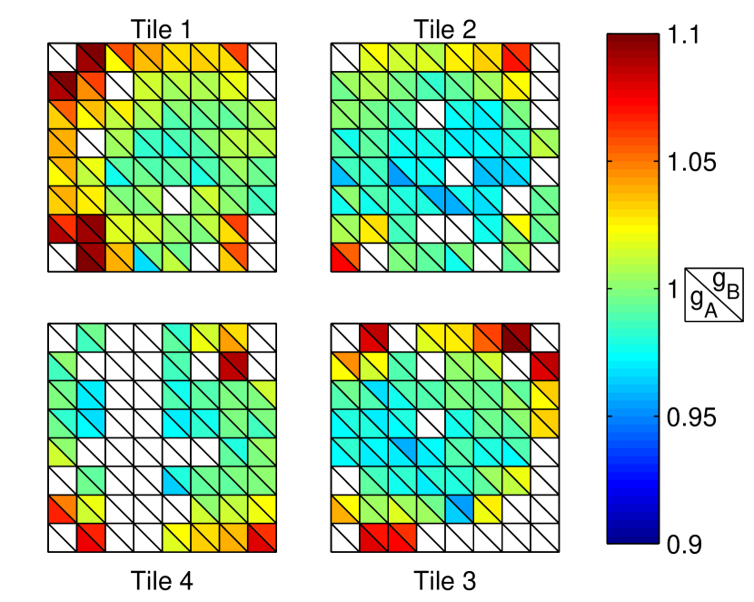
Figure 3.— Measured absolute gain for each detector included in Bicep2’s maps. The gains are normalized such that the median gain is one. The distribution within the focal plane is represented schematically. Each detector pair is depicted as a small square. The A (B) member of a detector pair is depicted as the lower (upper) triangle of the square.

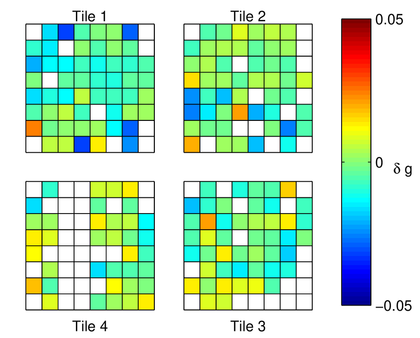
Figure 4.— Measured fractional differential gain, $(g_{A}-g_{B})/[g_{A}+g_{B})/2]$, for each detector pair included in Bicep2’s maps.

We emphasize that the deprojection algorithm described above does not require any external measurements of beam imperfections — the necessary coefficients, $a_{k}$, are fit for (marginalized over) from the CMB data itself. However, checking the operation of the technique and determining the residual contamination remaining after deprojection of any given set of modes requires external measurements of the actual instrument beams.

As summarized in Section 11.2 of the Instrument Paper, we have made high signal-to-noise beam maps of each detector by rastering the telescope over a chopped thermal source located $195$ m from the telescope’s aperture — for full details, see the Beams Paper. In this paper, we use these beam maps in two ways: (1) we fit elliptical Gaussians to them and cross check the fit parameters against those derived from the deprojection algorithm (Section 9.2), and (2) we use them as direct inputs to simulations to predict the T$\rightarrow$P leakage in the real data signal and jackknife maps while varying the set of modes deprojected (Section 10.1). Both offer highly robust checks that the beam maps correspond to reality.

During beam mapping, the instrument is put in a rather different state than that used for routine CMB observing, and the frequency spectrum of the source is not the same as that of the CMB. Beam shapes (especially differential beam shapes) and centroids are relatively insensitive to changes in the source spectrum, but differential gain — which typically arises from the coupling of intra-pair bandpass mismatch to the difference between the frequency spectrum of the atmosphere and the CMB — is not. Therefore, the differential gain measured in beam maps is not a reliable estimate of the CMB value. Instead we estimate it by cross-correlating single detector $T$ maps coadded over the full data set against the Planck 143 GHz map in a per-detector analog of the absolute gain calibration described in Section 13.3 of the Instrument Paper. Figure 3 shows the results, the measured absolute gain, $g$ for each of Bicep2’s detectors. Figure 4 shows the measured fractional differential gain for each of Bicep2’s detector pairs, $(g_{A}-g_{B})/[(g_{A}+g_{B})/2]$.

Differential pointing can be measured either from the beam maps or from the per-detector cross-correlation against the Planck 143 GHz maps described in Section 11.9 of the Instrument Paper. The results are very similar.

Figure 5 shows Bicep2’s differential pointing measured from per-detector cross-correlation, which shows a strong coherent component across the focal plane. The coherent part of the pattern will cancel in the final signal map and be enhanced in a $180^{\circ}$ split jackknife as described in Section 4.2.2. The incoherent part will average down in the signal map and also potentially cause jackknife failure.

Figure 6 shows Bicep2’s measured beam ellipticity and differential ellipticity. The differential ellipticity shows strong pair to pair variation in angle, so we expect some averaging down of leakage in the signal maps as described in Section 4.2.3. We also expect that jackknife tests that split the data according to pair will be sensitive to it.

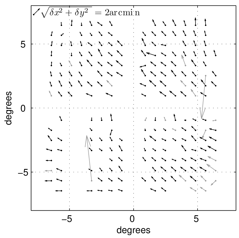
Figure 5.— Differential pointing in the Bicep2 focal plane as projected onto the sky at deck$=90^{\circ}$. As drawn, the vectors originate at the nominal beam center and point from detector B to detector A. Their magnitudes are drawn $\times 20$ for display purposes. All functioning pairs are plotted, but grayed out vectors indicate detector pairs that are excluded from the final maps.

Figure 6.— Top: per-detector beam ellipticity in the Bicep2 focal plane as projected onto the sky at deck$=90^{\circ}$. Ellipticity is exaggerated for clarity. Red and blue denote A and B members of a detector pair, respectively. All functioning pairs are plotted, but light colors indicate detectors that are excluded from the final map. Bottom: per-pair differential ellipticity, defined as $\sqrt{(\delta p)^{2}+(\delta c)^{2}}$. The orientation of the ellipse indicates the orientation of the difference beam quadrupole. Detector polarization angles are aligned with the horizontal and vertical axes.

7. Simulation pipeline

Bicep2’s power spectrum analysis is Monte-Carlo-based, requiring simulations of maps “as seen” by the experiment (Hivon et al., 2002). We simulate both noiseless (signal-only) and noise-only maps. The standard simulations introduced in Section V.A of the Results Paper include only differential pointing at the measured values shown in Figure 5. Here we extend the signal-only simulations to include many different types of systematics.

7.1. Input Maps and Interpolation

The simulation pipeline produces signal-only timestreams by sampling an input Healpix map along individual detectors’ trajectories. The simulated timestream data is then passed through the same map maker as the real data to produce simulated $T$, $Q$, and $U$ maps that are filtered identically to the data. Our pipeline extensions optionally introduce many different systematics at the timestream generation stage, allowing us to model their effects on the final maps.

Both the main simulations and our dedicated systematics simulations use input maps of Nside=2048. We perform the simulations of systematic T$\rightarrow$P using the Planck HFI 143 GHz $T$ map — pre-smoothed by Bicep2’s nominal, circular Gaussian beam as described in Appendix C.5 — as input. We use the downgraded resolution, Nside=512 version of the same map as the deprojection template. To predict T$\rightarrow$P, we set the input $Q$ and $U$ maps to zero so that any non-zero signal in the resulting polarization maps and spectra are due entirely to leakage. To simulate systematics that primarily leak E$\rightarrow$B we use as input maps synfast generated realizations of $\Lambda$CDM and do not set the $Q$ and $U$ maps to zero. We difference the spectra simulated with and without the systematic included and average over 10 realizations to estimate the E$\rightarrow$B leakage.

All the simulations except the beam map simulations described in Section 7.3 interpolate the input map to timestreams using a second order Taylor expansion around the $T$, $Q$, and $U$ pixel centers using the derivative maps that are a standard output of synfast. Assuming a polarization angle and efficiency, we combine a single detector’s $T$, $Q$, and $U$ timestream into a single timestream. Using simulated input maps of progressively higher resolution allows us to simulate timestreams to arbitrary accuracy. Doing this, we find that using an Nside=2048 map produces negligible fractional differences from a still higher resolution input map.

7.2. Elliptical Gaussian Beam Convolution

Leakage from differential pointing is naturally handled in all the simulations discussed above because each detector is allowed to have its own pointing trajectory on the pre-smoothed input maps.

In studies of systematics where we wish to vary the simulated elliptical Gaussian beam shape, we use multiple input maps which have each been pre-smoothed with circular Gaussians of different widths. Convolution on the sphere is fast and exact for any beam that is circularly symmetric (Wandelt & Górski, 2001).

To simulate beam widths that vary from detector to detector, we use a perturbative method in which two or more Healpix maps of bracketing widths are simultaneously read in and interpolated between at each time step to approximate the timestream from a beam of intermediate width. Using bracketing maps of closer and closer spacing allows simulation of differential beamwidth to arbitrarily high accuracy, which we use to verify that our choice of bracketing widths simulates leakage from beamwidth mismatch to sufficient accuracy.

Elliptical beam convolution is handled by approximating elliptical beams as the superposition of three or more circular sub-Gaussians of different widths, centers, and amplitudes, the choice of which is a function of $p$, $c$ and $\sigma$ and is predetermined from 2-d fits to elliptical Gaussians. Input maps pre-smoothed to different circular Gaussian widths are read in and each is interpolated along the sub-Gaussians’ trajectories. The individual timestreams are then combined to approximate the timestream from a detector with an elliptical Gaussian beam. The amplitudes, widths, and relative centers of the sub-Gaussians are fixed, but the orientation of the ellipse can vary along a scan trajectory according to the beam’s projected orientation. We have verified the accuracy of this approach with special simulations using intrinsically flat input maps and explicit 2D convolution. As with beamwidth, we can simulate elliptical beams to arbitrarily high accuracy using superpositions of greater numbers of circular Gaussians. Defining ellipticity $e=(\sigma_{maj}^{2}-\sigma_{min}^{2})/(\sigma_{maj}^{2}+\sigma_{min}^{2})$ we find that our procedure, which uses three Gaussians, produces timestreams from elliptical beams that are accurate for $e<0.15$.

7.3. Arbitrary Beam Shape Convolution

The preceding methods allow for nearly exact simulation of elliptical Gaussian beams. We also allow for arbitrary beam shape convolution.

We perform arbitrary beam shape convolution by forming a flat map projection of the input Healpix map, convolving this projection directly with a 2D kernel, and interpolating off the flat map to form simulated timestreams. We call these “beam map simulations.” Ordinarily, such a brute force algorithm would be very computationally expensive when simulating a large number of detectors observing over a long time period. For Bicep2 we have considerably reduced the expense by exploiting the fact that (1) the telescope’s deck angle remains fixed during CMB scans, (2) there is no sky rotation at the South Pole, and (3) Bicep2’s scan pattern is highly redundant. Thus, for a fixed deck angle, each detector observes a given location on the sky with only one orientation, and the convolution of the kernel with a flat sky map need only be performed once per detector per each of the four deck angles.

This method suffers from distortion away from the center of the projection. However, because the distortion is common to both members of a detector pair, the difference signal is still predicted with high accuracy. We test this by comparing the T$\rightarrow$P leakage simulated using the multiple Gaussian approach described in Section 7.2 (which, again, does not suffer from any flat sky distortion effects and which we perform to high accuracy) to beam map simulations that use as the convolution kernels elliptical Gaussians constructed to reflect identical beam parameters. Any difference in the T$\rightarrow$P leakage from the two methods is attributed to algorithmic limitations of the beam map simulation procedure. We have verified that the method of flat sky beam convolution is sufficient to accurately predict the level of leakage from all modes of an elliptical Gaussian, both before and after deprojection. These simulations make no assumptions of elliptical Gaussian beam structure, so this test verifies that beam map simulations will accurately predict T$\rightarrow$P leakage from arbitrary beam shape mismatch.

Deprojection is performed on these beam map simulations in the same way as in the standard simulations. Therefore, the leakage templates suffer from no corresponding distortion effects, and the main impact of projection distortion in beam map simulations is to slightly degrade the ability of deprojection to filter leaked power from the timestreams. This results in an artificial “floor” at $\simeq 10^{-5}~{}\mu$K² below which power due to the mismatch of elliptical Gaussians will not deproject in a beam map simulation. Beam map simulations thus always predict at least as much residual contamination as is present in the real data.

We have developed the beam map simulation procedure so that we can use measured beam maps as inputs. Because these empirical beam maps make no assumption of elliptical Gaussian structure, their ability to reproduce the behavior of real data spectra, both signal and jackknife, under different deprojection options is powerful evidence against residual, unmodeled, and undeprojected contamination from beam mismatch (see Section 10.1).

8. Jackknife tests

Bicep2’s most basic guard against systematics is jackknife tests (Pryke et al., 2009; Chiang et al., 2010). As already described in Section 2.3, we split the data into two subsets, form $T$, $Q$, and $U$ maps from each subset, and difference the maps. Under the hypothesis that the observed signal is real and “on the sky,” the difference map should be consistent with the distribution of systematics-free signal-plus-noise simulations. If some or all of the observed signal is from an instrumental systematic, then, depending on the type of hypothesized systematic, the different halves of a split will contain either different amplitudes or different spatial patterns of contamination. The Bicep2 jackknife tests were discussed in Section VII.C of the Results Paper. Here we review and give some fuller details.

Different jackknives probe for different classes of systematics. Some jackknives split the data according to the observing cycle, some according to detector pair selection, and one according to a combination of both. Detector pair selection jackknives are illustrated in Figure 7. Most systematics will produce different contamination in the two halves for at least one of the jackknife splits we form. The following is a description of Bicep2’s jackknives and the types of systematics that are expected to cause each to fail.

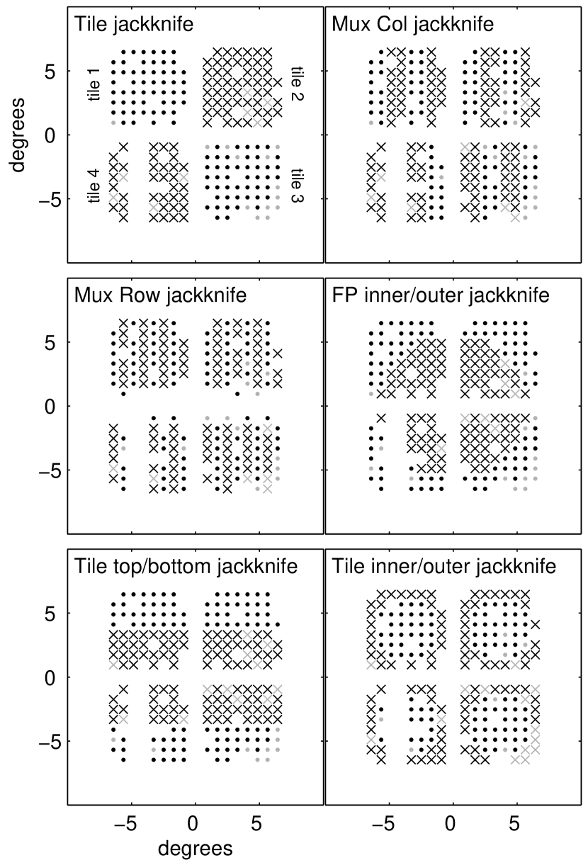
Figure 7.— Map of the Bicep2 focal plane projected onto the sky at deck$=90^{\circ}$ illustrating detector pair selection jackknife splits. Dots denote detector pairs that are coadded to form one half of the jackknife split; X’s denote detector pairs coadded to form the other half. All functioning pairs are shown. Light gray symbols indicate pairs that are excluded from the final map.

Deck angle:

Splits data according to boresight orientation, $68^{\circ}+113^{\circ}$ vs. $248^{\circ}+293^{\circ}$; highly sensitive to systematics that change sign under a rotation of the instrument, such as beam mismatch with dipolar symmetry (see Section 4.2.2). Because of this, Bicep2’s differential pointing contaminates the deck jackknife more strongly than the signal map (see Figure 8).

Alternative deck:

Same as deck, but $68^{\circ}+293^{\circ}$ vs. $113^{\circ}$ + $248^{\circ}$; similar to the deck jack, probes contamination that varies with boresight orientation.

Temporal split:

Splits data into equal weight halves by date; sensitive to any long-term drifting of instrument properties.

Scan direction:

Splits data according to the telescope scanning direction, left-going vs. right-going; sensitive to detector transfer function mismatch. T$\rightarrow$P leakage from transfer function mismatch contaminates the scan direction jackknife more strongly than the coadded map. Because it is the jackknife with the lowest predicted residuals, it is also the jackknife most sensitive to noise model errors.

Azimuth:

Splits data according to interleaved 10 hr blocks of time (phases) within the three-day observing cycle (phases B+E+H vs. C+F+I; see Section 12.3 or Table 6 of the Instrument Paper for details). Because these phase groups are offset from each other in azimuth, this jackknife probes azimuth fixed contamination, such as would be expected from polarized ground pickup.

Moon up/down:

Splits according to times when the moon is above vs. below the horizon; sensitive to contamination due to the moon.

Tile:

Splits data by detectors, tiles 1+3 vs. tiles 2+4; sensitive to differences in detector properties, e.g. bandpass.

Tile/deck:

Tiles 1/2 at deck $68^{\circ}$/$113^{\circ}$ + tiles 3/4 at deck $248^{\circ}$/$293^{\circ}$ vs. tiles 1/2 at deck $248^{\circ}$/$293^{\circ}$ + tiles 3/4 at deck $68^{\circ}$/$113^{\circ}$; sensitive to effects that are common between tiles. (Rotating the receiver by $180^{\circ}$ places new tiles at a given projected location on the sky. However, the physical orientations of tiles 1 and 2 as installed in the focal plane are rotated $180^{\circ}$ from tiles 3 and 4, so that the new tiles have the same projected orientation after rotation. Thus, the regular deck jackknife does not directly probe for tile fixed effects that are common among tiles.) Because Bicep2’s instantaneous field of view is large compared to the map area, this jackknife map has smaller useful coverage than the other jackknives.

Focal plane inner/outer:

Splits according to the inner 50% of detectors vs. the outer 50% of detectors in the focal plane; sensitive to beam shape mismatch that varies with distance from the center of the focal plane, as would be expected of ellipticity induced by variable beam truncation in the aperture plane.

Tile top/bottom:

Splits according to top of each tile vs. bottom of each tile, where the sense of top and bottom is defined with respect to the tile as fabricated, not globally within the focal plane; sensitive to effects that vary within an individual tile.

Tile inner/outer:

Splits according to the inner 50% vs. the outer 50% of detectors within a tile; sensitive to effects that vary within an individual tile.

Mux column:

Splits according to detector multiplexing column, even vs. odd; sensitive to crosstalk contamination.

Mux row:

Splits according to detector multiplexing row.

Differential pointing best/worst:

Splits according to the 50% of detector pairs with the smallest differential pointing and the 50% of detector pairs with the greatest differential pointing. Like the deck and alt deck jackknives, it is more sensitive to differential pointing contamination than the signal maps.

Table 1 of the Results Paper lists probability to exceed (PTE) values for four statistics, computed separately for the $EE$, $BB$, and $EB$ spectra, for each of the above 14 jackknife spectra. There are thus 168 PTE statistics but some of these are partially correlated. There is one $BB$ or $EB$ PTE with a value $\leq 0.01$, the mux row $BB$. Of the 499 $\Lambda$CDM signal + noise simulations used in the main analysis (which should reproduce the correlations), 306 realizations have one or more $BB$ or $EB$ PTE $\leq 0.01$ so this is unsurprising. The real data contain six $EE$ PTEs $\leq 0.01$. Of the 499 simulations, 2 have 6 or more $EE$ PTEs $\leq 0.01$.

The Results Paper offers an explanation for the apparently anomalous number of low $EE$ PTEs: because of the high signal-to-noise of Bicep2’s $EE$ measurements, variation in the mean gain from detector pair to detector pair results in failures of the detector selection jackknives shown in Figure 7. The $BB$ detection is, of course, highly significant as well, but the $EE$ signal-to-noise ratio, which is $\sim 500$ at $\ell=100$, makes even the smallest absolute calibration difference between jackknife halves impact the PTE, even though such absolute calibration errors do not imply systematic contamination of the signal map. We include this effect in 10 of the signal simulations by multiplying each detector pair’s data by the mean of its measured absolute gain, $(g_{A}+g_{B})/2$, shown in Figure 3 (see Section 10.3). The difference of the $EE$ spectra with and without gain variation is an estimate of the contaminating power, and is $\simeq 1\times 10^{-3}~{}\mu$K² at $\ell=100$. Including this contaminating power results in 9 of the 499 realizations having six or more $EE$ PTEs $\leq 0.01$. Gain variation is not important for jackknives of the comparatively low signal-to-noise $BB$ data.

9. Deprojection Performance

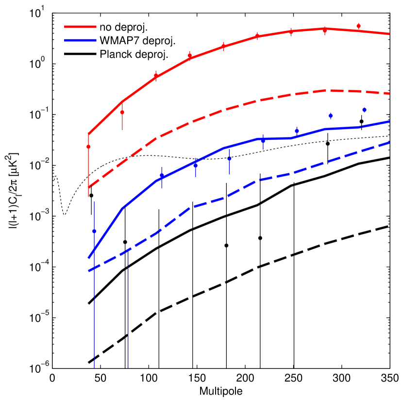
Figure 8.— Points with error bars are Bicep2’s deck jackknife bandpowers with (red) no deprojection, (blue) differential pointing deprojected with a WMAP7 V-band template, and (black) differential pointing deprojected with a Planck 143 GHz template, with error bars taken as the standard deviation of $\Lambda$CDM plus instrumental noise simulations that include Bicep2’s measured differential pointing. The solid lines are the corresponding simulated deck jackknife spectra, computed as the mean of 50 noiseless simulations of $\Lambda$CDM $T$ and Bicep2’s measured differential pointing, deprojected with templates containing simulated template noise. The dashed lines show the corresponding simulated non-jackknife, signal $BB$ leakage. The dotted line shows a lensed $\Lambda$CDM + $r=0.2$ spectrum for reference.

We characterize the performance of deprojection by specifying the residual spurious power remaining in Bicep2’s polarization power spectra after deprojection. We split this characterization into two parts. First, we approximate the beams as elliptical Gaussians and determine the residual contamination from various mismatch modes using the simulations introduced in Section 7.2. This serves as a test of deprojection’s fundamental limit. Second, we use the beam map simulations described in Section 7.3 to determine the actual residual contamination after deprojection, including that from the portion of Bicep2’s beams not described by elliptical Gaussians. In this section, we deal only with the first characterization. The second is described in Section 10.1.

9.1. Template Map Non-idealities

We first consider how non-idealities in the deprojection template map limit the efficacy of deprojection. By far, the most important non-ideality is simply statistical noise in the deprojection template. We have deprojected Bicep2 data with two different templates — a WMAP7 V-band (Jarosik et al., 2011) and a Planck HFI 143 GHz $T$ map (Planck Collaboration et al., 2014b) — which have different bandpasses and different noise properties. We have also performed timestream simulations using the measured elliptical Gaussian parameters discussed in Section 6 and deprojected them with templates containing simulated Planck and WMAP noise. (We describe the construction of simulated template maps in Appendix C.5.)

These simulations predict that Bicep2’s differential pointing is by far the dominant source of contamination in the deck jackknife, and the dominant source of contamination in the signal spectra prior to deprojection. Furthermore, as expected given the discussion in Section 4.2.2 and the substantially coherent measured differential pointing shown in Figure 5, the deck jackknife spectrum is far more contaminated by differential pointing than the signal spectrum.

We isolate the effect of differential pointing by simulating it separately from other difference beam modes. Because we want to investigate the impact of template map noise, we simulate T$\rightarrow$P leakage using noiseless realizations of $\Lambda$CDM $T$ as input and noise added versions of those same maps, downgraded to Nside=512, as the deprojection templates. Figure 8 shows the results as well as real data for Bicep2’s deck jackknife. In these simulations, the efficacy of deprojection is entirely determined by the level of noise in the template map. The predicted contamination in the signal spectrum after deprojection with either the WMAP7 or Planck template (dashed blue and black lines) is small compared to an $r=0.2$ IGW spectrum at $\ell<150$. However, when deprojecting with the noisier WMAP7 template, the T$\rightarrow$P leakage in the deck jackknife (solid blue line) is measurable and well predicted by simulation. Because the deck jackknife has much greater contamination than the signal spectrum, it is a highly stringent test of contamination. Our accurate prediction of residual contamination in the deck jackknife is strong evidence against significant unmodeled leakage in the signal maps. In Bicep2’s main results, deprojection is performed with a Planck 143 GHz template, and T$\rightarrow$P leakage from differential pointing is negligible and unmeasurable in even the deck jackknife.

We note that bandpass differences between Bicep2 and the deprojection template are not important. The WMAP V-band template is centered at 60 GHz while the Planck template is centered at 143 GHz, much closer to Bicep2’s central frequency. In principle, the T$\rightarrow$P leakage at different frequencies is not the same because of unpolarized foregrounds with non-CMB-like spectral dependencies. The agreement of the data points and the solid lines in Figure 8 indicates that for even significant bandpass differences, undeprojected leakage from foregrounds not present in the deprojection templates is negligible. Foregrounds present in the deprojection template that are fainter in Bicep2’s band would be a source of unmodeled template noise, which Figure 8 indicates is also not an issue. We have also simulated adding point sources to the template map that are not present in simulated Bicep2 maps, and this also has a negligible effect on deprojection.

9.2. Consistency With Beam Maps

We confirm that deprojection filters contamination consistent with our measured difference beams by comparing the differential beam parameters implied by the deprojection fit coefficients of Bicep2’s real data (calculated according to Table 3) to the independent measurements of the same parameters described in Section 6. Figure 9 shows the correlation of the deprojection derived differential beam parameters with the beam-map-derived differential beam parameters. (Note that $\delta x$ and $\delta y$ are measured from beam maps, not from correlation of per-detector $T$ maps with Planck maps, as in Figure 5, and are thus fully independent of the deprojection coefficients, if somewhat lower signal-to-noise.) The uncertainties of the beam-map-derived parameters are somewhat difficult to accurately estimate. However, the scatter in the observed relation is consistent with the scatter on the deprojection coefficients predicted from signal-plus-noise simulations, indicating that noise in the CMB data dominates the scatter in Figure 9.

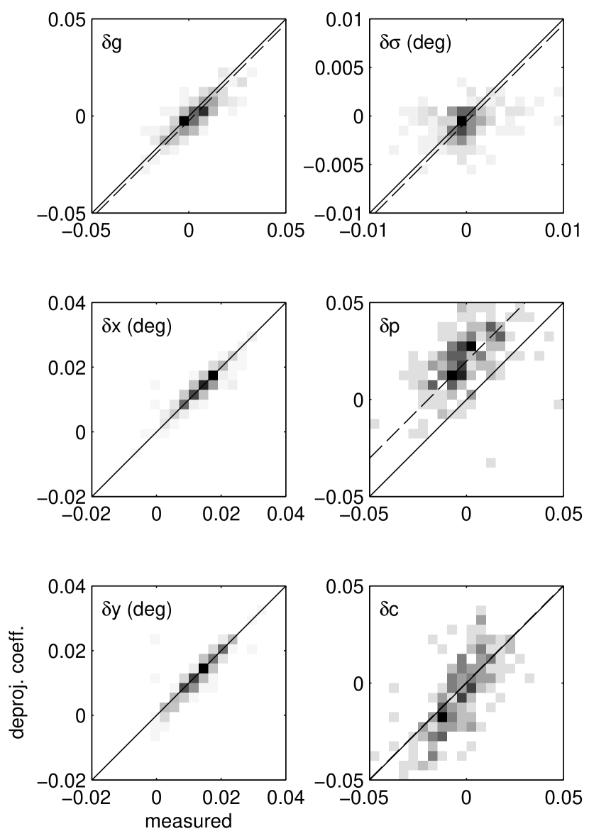
Figure 9.— Differential beam parameters measured from far-field beam maps (horizontal axis) and from template regression as used in deprojection (vertical axis), shown as 2D histograms over detector pairs. (Differential gains are determined from cross-correlation of individual detector T maps with Planck.) The solid line has a slope of 1 and a $y$-intercept of 0. The dashed line has slope of 1 but has been offset vertically by the bias in the recovered deprojection coefficients predicted from simulation. The scatter and bias in the observed relation is broadly consistent with that predicted from signal-plus-noise simulations.

The significant bias visible in the plus-ellipticity deprojection coefficient results from the inherent $TE$ correlation in $\Lambda$CDM cosmology, which ensures some correlation between the true CMB polarization signal and the deprojection templates. This bias does not impair the filtering of T$\rightarrow$P leakage, but it does cause additional filtering of cosmological $E$-modes (the effect on $B$-modes is negligible). The effect on both $E$-modes and $B$-modes is automatically accounted for in the filter/beam suppression factors derived from simulations that apply the same choice of deprojection (see Section  VI.C of the Results Paper). We have verified that the bias arises from $\Lambda$CDM $TE$ correlation by observing that the bias disappears in simulations with no $TE$ correlation.

Given good agreement between measured differential beam parameters and those inferred from deprojection, we can choose to either deproject a given differential mode or to subtract the contamination expected given our direct measurements. Differential gain can, in principle, have a significant time variable component, so we choose to deproject it. (We perform the deprojection regression on approximately 9 hr chunks of data; see Appendix C.5 for details.) Differential pointing is measured with high signal-to-noise in beam maps and is expected to be constant in time, but because it is Bicep2’s largest source of T$\rightarrow$P leakage we conservatively choose to deproject it to avoid any residual leakage arising from noise in the calibration measurements. Since differential ellipticity deprojection preferentially filters our $TE$ and $EE$ spectra, we choose to fix the deprojection coefficients to the beam-map-derived values and subtract the scaled deprojection templates from the data, rather than fitting the templates. In the results of the beam map simulations described in Section 10.1, we find this to be empirically equivalent to deprojecting ellipticity

The simulation of Bicep2’s best-fit elliptical Gaussian beam shapes that include all six differential modes demonstrates that T$\rightarrow$P leakage from pure elliptical Gaussian mismatch can be cleaned to the $r\sim 1\times 10^{-4}$ level with deprojection using a template with Planck 143 GHz noise levels. At this level, the component of Bicep2’s beam mismatch not fit by the difference of elliptical Gaussians is the dominant source of T$\rightarrow$P leakage.

10. Systematics error budget

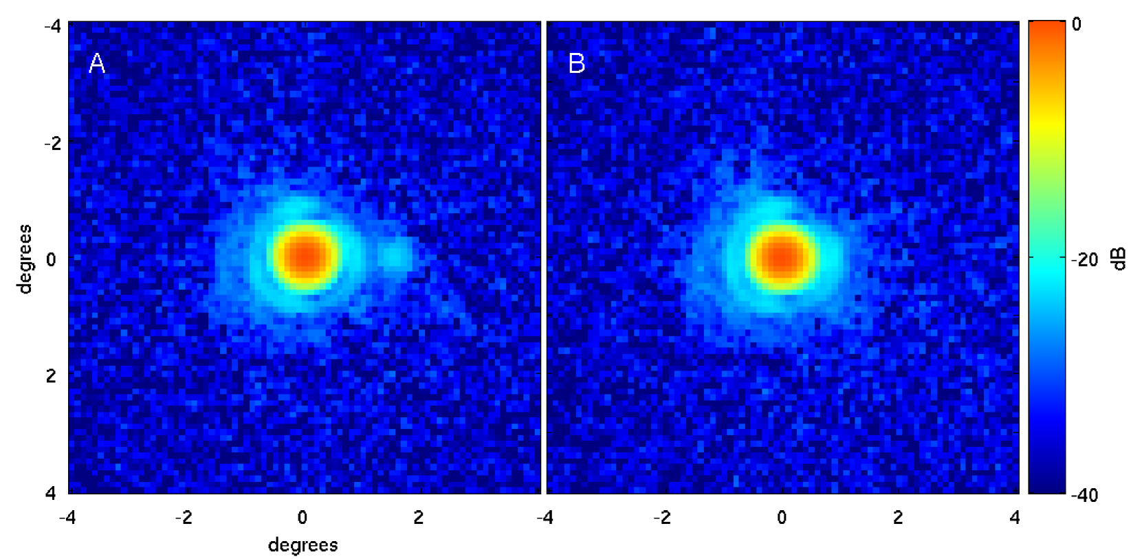
Figure 10.— Composite beam map for a representative detector pair, showing the A and B beams. ($1~{}\mbox{dB}=10\log_{10}$.) The coordinate system is centered on the mean pair centroid. The expected crosstalk feature with $\sim-25$ dB amplitude is visible in the A detector on the horizontal axis at a distance of $\sim+1.7^{\circ}$ from the beam center. The first Airy ring is visible at a radius of $\sim 1^{\circ}$. The difference beam (not shown) is dominated by a dipole structure.

Jackknife tests fail when the magnitude of contamination exceeds the noise in the jackknife maps, which, in general, is comparable to the noise in the signal maps. If the contamination is uncorrelated in the two halves of the jackknife split, then jackknife tests can place upper limits on possible contamination only as low as the level of Bicep2’s statistical uncertainty. We therefore rely on the jackknife tests described in Section 8 primarily as a safeguard against unknown and unmodeled systematics. Using special calibration data, we constrain known possible systematics to much lower levels.

In this section, we use a few approaches to either directly determine or place upper limits on the contamination from a given systematic. First, where a systematic is strong enough relative to the sensitivity of calibration data, we directly determine the $BB$ spectrum of the expected spurious signal using simulations of the effect. Many of the calibration measurements are described in the Instrument Paper, and are similar to those described in Takahashi et al. (2010). Second, where calibration data exist but the systematic effect in question is not large enough to directly measure, we place upper limits on the contamination given the sensitivity of the calibration data. Third, in the absence of robust calibration data, we can determine the level of a hypothesized systematic that would show an observable effect in Bicep2’s signal and jackknife spectra and set an upper limit this way.

We quote the level of contamination from individual sources of systematics by assigning a characteristic tensor/scalar ratio to the spurious $BB$ power they generate. We compute this characteristic $r$-value using the “direct likelihood” method developed in Barkats et al. (2014) and used in Section  XI.A of the Results Paper. We first compute a weighted sum of bandpowers of the predicted spurious signal. We use signal/variance weighting, with a signal equal to an $r=0.1$ IGW spectrum and variance equal to the variance of bandpowers from simulations of lensed-$\Lambda$CDM signal + instrument noise. The ratio of this weighted sum (multiplied by $0.1$) to the identically weighted sum of a pure $r=0.1$ IGW spectrum is the characteristic $r$-value of the contamination. (In practice, the choice of fiducial $r$ makes no difference.)

Because this procedure strongly de-weights bandpowers above $\ell\simeq 120$, contamination at these multipoles will not be reflected in the quoted $r$-values. Nonetheless, we plot systematics spectra at $\ell<350$ and can therefore verify that systematics are small at all scales presented in the main analysis.

10.1. Undeprojected Residual Beam Mismatch

In Section 5, we described the deprojection algorithm that allows us to filter out T$\rightarrow$P leakage from mismatched beams and in Section 9 demonstrated that for idealized elliptical beams the residual T$\rightarrow$P contamination after deprojection using the Planck 143 GHz template map is well below Bicep2’s noise. Because deprojection, as parametrized, filters only power corresponding to the modes of the difference of elliptical Gaussians, the portion of any detector pair’s difference beam not described by this model creates residual, undeprojected contamination.

As described in Section 6 and in the Beams Paper, we have obtained high signal-to-noise beam maps of every Bicep2 detector. The source was observed 3 times each at 4 deck angles to produce a total of 12 individual $8^{\circ}\times 8^{\circ}$ beam maps for each detector. The central region of each detector’s beam map, at radius $r\leq 1.2^{\circ}$, is covered by all 12 observations. This area contains $97\%$ of the total integrated beam power. The regions of the beams at $r>1.2^{\circ}$ are not fully covered by observations at a single deck angle. Beam map pixels at $r\leq 3^{\circ}$ from the beam center are observed at a minimum of two deck angles. Regions of the beam map at $r>3^{\circ}$ are generally observed at a single deck angle.

We combine the available observations to form one composite beam map for each detector. We do this in two ways: (1) we median filter the full beam maps to produce $8^{\circ}\times 8^{\circ}$ maps, and (2) we set to zero the portion of the beam maps at $r>1.2^{\circ}$ and mean filter the observations. We refer to these two composite maps as the (1) extended and (2) main beams. The median filter is necessary for the outer regions of the beam maps because of artifacts in some of the observations. The extended composite beam map for a representative detector pair is shown in Figure 10.

We apply a gain mismatch by normalizing each detector’s beam map to reflect the differential gain measurements shown in Figure 4. (We normalize each detector pair’s two beam maps such that the mean gain is one and the intra-pair ratio of the mean of the square root of the azimuthally averaged beam window functions, $B_{\ell}$, in the multipole range $100<\ell<300$ equals the ratio of the measured absolute gains. This procedure ensures we apply the differential gain in simulation to the same multipole range as in which it was measured.)

10.1.1 Undeprojected Residual in Signal Maps

We use these beam maps as inputs to the beam map simulation algorithm described in Section 7.3 and compare the resulting T$\rightarrow$P leakage to the real data.

The left panel of Figure 11 shows the predicted $BB$ contamination from the main beam map simulations using different deprojection options. The colored bands indicate the $\pm 1\sigma$ uncertainty of the predicted leakage, which is set by noise in the beam maps and the absolute gain measurement uncertainty. The top right panel of Figure 11 shows the change in simulated leakage when applying deprojection as colored bands, as well as the observed change in Bicep2’s bandpowers under different choices of deprojection as points. Again, the shaded bands indicate the $\pm 1\sigma$ uncertainty of the beam map simulations. The error bars on the points are the standard deviation of bandpower differences from simulations that include lensed-$\Lambda$CDM signal and instrumental noise. The details of the estimation of the leakage uncertainty are given in Appendix D.

Figure 11 shows that deprojection of differential pointing is absolutely necessary and differential gain is also important. Differential ellipticity is a smaller effect. Once these deprojections are in effect the residual contamination is seen to be very small.

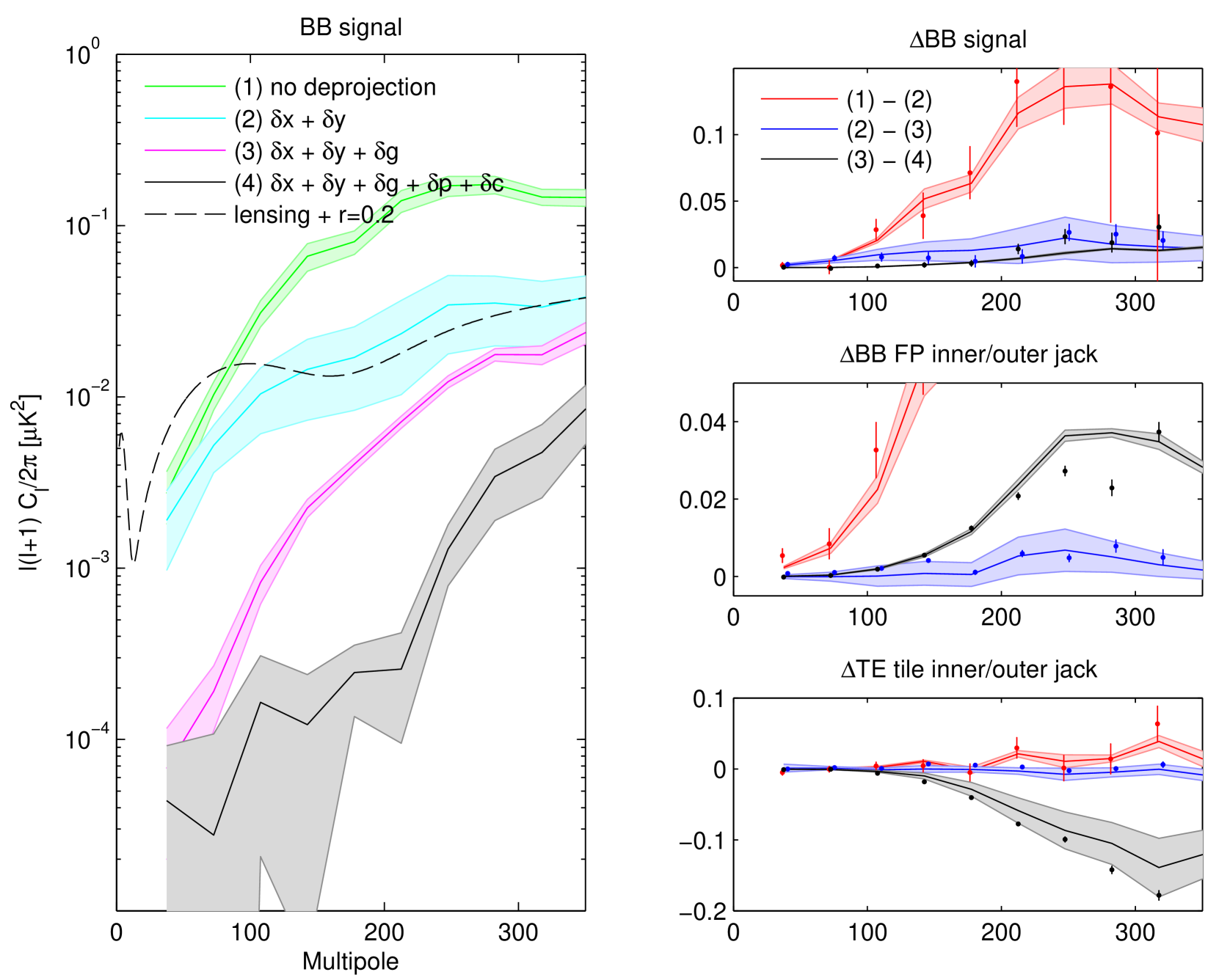
Figure 11.— Left panel: $BB$ contamination predicted from beam map simulations of Bicep2’s measured main beams (temperature only simulations using the Planck HFI 143 GHz $T$ map convolved with measured, per-detector beam maps). The shaded bands indicate the $1\sigma$ uncertainty of the contamination given the sensitivity of the beam maps and gain mismatch measurements. The colors correspond to different choices of deprojection: (1) no deprojection; (2) deprojection of differential pointing ($\delta x+\delta y$); (3) deprojection of differential pointing and differential gain ($\delta x+\delta y+\delta g$); and (4) deprojection of differential pointing, differential gain, and differential ellipticity ($\delta x+\delta y+\delta g+\delta p+\delta c$). Right panels: Changes in bandpowers with different deprojection choices for: (top) the $BB$ signal spectrum, (middle) the $BB$ focal plane inner/outer jackknife, and (bottom) the $TE$ tile inner/outer jackknife. The solid lines and shaded bands again indicate the mean and $1\sigma$ uncertainty of the predicted leakage given the sensitivity of the beam maps and gain mismatch measurements. The points with error bars are the real data bandpower differences, with error bars computed as the rms of Bicep2’s standard, lensed-$\Lambda$CDM signal plus instrumental noise simulation set.

10.1.2 Undeprojected Residual in Jackknife Maps

We can further compare the action of deprojection on real data and simulations for each of the jackknives described in Section 8. As described in Section 4, some beam systematics undergo considerably less averaging down due to incoherence across the focal plane and cancellation due to instrument rotation in certain jackknifes. In these cases, we can investigate the behavior of deprojection in circumstances where it has to “work harder” than in the full signal map.

Examples of this are the focal plane inner/outer and tile inner/outer splits illustrated in Figure 7. As seen in Figure 6 Bicep2’s beam ellipticities exhibit a dependence on distance from the focal plane center while the differential ellipticity is strongest around the edges of individual tiles. The right center panel of Figure 11 shows that the focal plane inner/outer jackknife has a much stronger response in $BB$ to differential ellipticity deprojection than the full signal map, and that the degree of this response matches between real data and simulations. Likewise, the bottom right panel shows that the tile inner/outer jackknife responds as predicted in the $TE$ spectrum.

In general the simulated jackknife residuals match the real data for all the jackknives, under all deprojection combinations. Even without differential ellipticity deprojection, the contamination of the $BB$ spectrum is negligible, yet we still detect it in the jackknives that ought to be most sensitive to it. These many additional tests build confidence that we understand T$\rightarrow$P leakage from beam shape mismatch to an accuracy and precision surpassing that required by our error budget.

10.1.3 Undeprojected Residual Correction

The simulated main beam leakage with differential gain, pointing and ellipticity deprojection is robustly measured and is shown as the black line in the left panel of Figure 11. This leakage corresponds to $r=1.1\times 10^{-3}$ and is subtracted from the $BB$ bandpowers prior to fitting $r$ in Section  VIII.A of the Results Paper. The expected main beam contamination in the final results is therefore zero.

The extended beam simulations are noisier than the main beam simulations and the median filter makes statistics derived from them less robust. The predicted extended beam leakage is consistent with zero and we adopt its $1\sigma$ uncertainty as the upper limit of possible remaining T$\rightarrow$P leakage from beam shape mismatch after the main beam residual correction. Because the extended beam maps include the main beam, this upper limit includes the uncertainty of the residual leakage correction. Moreover, because the extended beam maps include crosstalk beams, it includes T$\rightarrow$P leakage from multiplexer crosstalk. The upper limit is shown in Figure 13 and indicates that beam shape mismatch contributes T$\rightarrow$P leakage corresponding to $r<3.0\times 10^{-3}$.

10.2. Further Consideration of Gain Mismatch

Deprojection filters T$\rightarrow$P leakage from gain mismatch with such effectiveness that the subtle choices of multipole ranges and normalization constants described in Section 10.1 make virtually no difference. We have simulated up to three times the level of measured relative gain mismatch and found no change in the predicted residual contamination after deprojection. The “extended beam” upper limit in Figure 13 includes contamination from gain mismatch.

Other lines of evidence against systematic contamination by gain mismatch are the cross-spectrum of Bicep2 and Bicep1, and the passing of jackknives. Because we calibrate the relative response of our detectors hourly by executing elevation dips (the “el nods” described in Section  12.4 of the Instrument Paper) and observing the large response from changing atmospheric loading, we expect that a gain miscalibration will primarily be the result of intra-pair bandpass mismatch coupling to differences between the color spectrum of the CMB and the atmosphere at the South Pole (Bierman et al., 2011). As discussed in Section 4.2.1, it is only coherent gain mismatch that will evade Bicep2’s jackknife tests. Because Bicep1 and Bicep2’s bandpasses are physically defined in very different ways (horn and mesh filter vs. antenna and lumped-element filter), we expect that a coherent mismatch will not correlate between the two experiments.

Also as discussed in Section 4.2.1, while coherent differential gain will not contaminate jackknives in Bicep2, it will (1) contaminate jackknives in Bicep1, and (2) contaminate the signal map differently in Bicep1 because of the different layout of polarization angles. Thus, while the power spectrum of contamination from uniform gain mismatch could be similar in Bicep1 and Bicep2  correlation would not be expected. Thus, the consistency of the Bicep1$\times$Bicep2 cross-spectrum with the Bicep2 auto spectrum as presented in Figure 7 of the Results Paper is evidence against residual uniform gain mismatch. Incoherent gain mismatch is still expected to contaminate pair selection jackknives. Additionally, a coherent gain mismatch common to Bicep2 and to the Keck Array will not produce correlated power. In Keck Array maps from 2013 and after, a coherent gain mismatch will fully cancel in signal maps as well as contaminate $90^{\circ}$ split jackknives.

10.3. Gain Variation

Bicep2 applies a single absolute calibration to the final coadded maps. Because the map coverage region is not the same for all detector pairs, a variation of mean gain from pair to pair will cause E$\rightarrow$B leakage, even if the intra-pair differential gain is zero.

The matrix-based map purification discussed in Section  VI.B of the Results Paper ensures that the E$\rightarrow$B leakage from timestream filtering and map apodization is at a level corresponding to $r<10^{-4}$. We simulate E$\rightarrow$B leakage from gain variation within the focal plane by applying the per-pair mean of the absolute gains shown in Figure 3 to signal-only simulations containing unlensed $\Lambda$CDM $E$-mode power. The accuracy of this procedure is limited by the matrix purification, and so is an upper limit. We find that gain variation within the focal plane contributes E$\rightarrow$B leakage corresponding to $r<5.3\times 10^{-5}$.

A separate issue is temporal gain variation. Temporal gain variation per se is not a systematic (the full season coadded maps are calibrated against Planck), nor is static differential gain or temporal variation of differential gain on timescales longer than $\sim 9$ hr, the timescale over which we perform the fit of the deprojection templates to the data (see Appendix C.5). However, temporal variation of the differential gain on timescales shorter than the 9 hr deprojection timescale will produce T$\rightarrow$P leakage that does not fully deproject. We therefore reject $\sim 1$ hr blocks of data (“scansets”) from channels whose el-nod-derived gains change by more than $30\%$ as measured at the beginning and end of the scanset, and reject pairs whose ratio of gains changes by more than $10\%$ (see Section 13.7 of the Instrument Paper). As discussed in Appendix C.5 and in Section  IV.F of the Results Paper, the deprojection timescale was chosen as a compromise between the desire for robustness against temporal variation of sytematics (favoring shorter timescales) and the desire to minimize unnecessary filtering of signal (favoring longer timescales). We note that before this timescale was settled upon, the power spectrum results using deprojection performed on hour-long timescales were consistent with those using deprojection performed on 9 hr long timscales, modulo the additional E$\rightarrow$B variance resulting from the more aggressive filtering. We regard this as empirical evidence against the existence of leakage from unknown temporal differential gain variation at relevant levels.

10.4. Crosstalk

The leakage from the forms of crosstalk we expect in Bicep2 (Brevik, 2012) is easily incorporated into our simulation pipeline. The simulated timestreams from a detector’s multiplexer neighbors are simply multiplied by constants reflecting the level of crosstalk and added to the detector’s timestream. We have measured levels of crosstalk between channels in a variety of ways: first, we use cosmic ray hits on the focal plane that induce large changes in the signal on a given detector to map out the relative pickup on other detectors, yielding a non-symmetric $N_{\mathrm{detector}}\times N_{\mathrm{detector}}$ matrix of crosstalk coefficients. Second, we determine crosstalk coefficients for nearby detectors by cross-correlating individual detector CMB $T$ maps offset by the known angular distance to the channel next to it in the multiplexing ordering scheme. Third, we determine the crosstalk from nearby detectors by fitting a 2D Gaussian to the secondary beams that are seen with high signal-to-noise in individual detector beam maps, such as in Figure 10. Fourth, we have extended the deprojection algorithm to remove crosstalk leakage. (We do this by fitting the differential gain leakage template of a detector pair’s two multiplex neighbors to that detector pair; averaging the coefficients over three years is a measure of the crosstalk coefficient.)

Crosstalk T$\rightarrow$P leakage will partially cancel when coadding detectors within a multiplexing column into maps (Sheehy, 2013). Detector pairs that are nearest neighbors in the multiplexing ordering scheme are second nearest neighbors in the physical layout of the focal plane. Incrementing in multiplex samples, every other detector along a physical row is first sampled, then the interleaved detectors are sampled in the reverse physical direction. As a consequence, the crosstalk induced T$\rightarrow$P leakage on two physically adjacent detector pairs is equal in magnitude but opposite in sign when they are pointed at the same location on the sky. If the crosstalk coefficient is the same for all detectors, the leakage almost fully cancels when adding the data from adjacent pairs to form maps. Timestream simulations confirm that the cancellation mechanism is highly effective as long as the average crosstalk is similar between channels upstream in the multiplexing order and channels downstream in the multiplexing order, which our various measurements indicate is the case.

Direct simulations of crosstalk coefficients derived using all of the methods described above predict similarly small levels of T$\rightarrow$P leakage. The least noisy and most easily interpretable of these methods is the fitting to beam maps. Simulation of the measured per-pair crosstalk, which has a median of $\simeq 0.3\%$, predicts leakage corresponding to $r\simeq 3.2\times 10^{-3}$, which we adopt as the predicted systematic contamination.

10.5. Ghost Beams

In addition to the $8^{\circ}\times 8^{\circ}$ beam maps described in Section 10.1, we map the beam response out to radius $\sim 20^{\circ}$ using a bright non-thermal source. We observe a small-amplitude “ghost beam” for each detector located at the position of that detector’s beam reflected across the boresight axis. These likely result from reflections in the optics chain. The peak amplitude of these ghost beams is small, $\simeq 4\times 10^{-4}$ relative to the main beams. We can detect them because in the large beam maps we use a brighter microwave source than that used for the main and extended beam maps. We fit and measure the differential elliptical Gaussian parameters of these ghost beams, which are generally different from those of the corresponding main beam. We directly simulate the T$\rightarrow$P leakage from mismatched ghost beams by using the elliptical Gaussian convolution approach described in Section 7.2. The predicted leakage is small, corresponding to $r\simeq 7.2\times 10^{-6}$.

10.6. Polarization Angles

We divide the residual E$\rightarrow$B leakage from polarization angle miscalibration into a systematic (fully coherent) and a random component.

10.6.1 Systematic Polarization Angle Error

Section VIII.B of the Results Paper describes Bicep2’s procedure for self-calibrating the overall polarization angle orientation of the detectors, which removes the systematic component. Summarizing this procedure, we find that, prior to calibration, the high-$\ell$ $TB$ and $EB$ spectra are consistent with a coherent $-1.1^{\circ}$ polarization angle error and apply an equal and opposite rotation to the polarization maps prior to computing power spectra. Doing so filters the E$\rightarrow$B leakage from a systematic polarization angle error. Given the analytic expression for E$\rightarrow$B leakage found in Equation 5 of Keating et al. (2013) and assuming a $\Lambda$CDM $EE$ spectrum, we then calculate the maximum possible residual miscalibration by determining the coherent rotation at which Bicep2’s $TB$ and $EB$ spectra would show significant non-zero power. For coherent angle errors $\ll 1$ rad, the contamination of $BB$ scales quadratically with the angle error, while contamination of $TB$ and $EB$ scales linearly. The $TB$ and $EB$ spectra are therefore contaminated more strongly than $BB$ for a given angle error, and the resulting upper limit on $BB$ contamination is negligible. Given the sensitivity of Bicep2’s $TB$ and $EB$ spectra, a systematic polarization angle rotation of $0.20^{\circ}$ produces a failure of the $EB$ $\chi$ statistic, which tests for coherently positive or negative residuals (and is defined in Equation 8 of the Results paper) in $95\%$ of Bicep2’s signal-plus-noise simulations, which limits the possible E$\rightarrow$B leakage to $r<4.0\times 10^{-4}$.

10.6.2 Random Polarization Angle Error

Self-calibration removes the leakage from a systematic error in polarization angle, but errors in relative polarization angles between detectors still produce additional E$\rightarrow$B leakage. We measure detector polarization angles with a dielectric sheet calibrator (Takahashi et al., 2010). The measurements are described in detail in Section  11.4 of the Instrument Paper. After accounting for the $-1.1^{\circ}$ systematic rotation, the difference between the measured and nominal polarization angles is small. The distribution is approximately Gaussian, with an rms of $0.14^{\circ}$. We have estimated that the precision of these measurements is $\sim 0.2^{\circ}$ (Aikin, 2013), so the relative misalignment of individual detector polarization angles is not measured with high significance.

Leakage from random polarization angle errors is easily simulated. We simply assume one set of per-detector polarization angles in the simulation stage and use another in the map making stage. The resulting $Q$ and $U$ maps contain $\Lambda$CDM $E$-mode power that has been rotated into $B$-mode power. The difference between spectra estimated from maps made with the “wrong” polarization angles and the known, “correct” polarization angles is the E$\rightarrow$B leakage from polarization angle error. Simulation of the E$\rightarrow$B leakage from a random polarization angle error of $0.2^{\circ}$ rms predicts contamination corresponding to $r\lesssim 5.0\times 10^{-5}$.

10.7. Cross-polar Response

In addition to the miscalibration of the polarization angle, there can be higher order cross-polar response terms in the beam that give rise to E$\rightarrow$B leakage. If a pair that is analyzed assuming it responds only to $Q$ polarization actually has some response to $U$, there will be polarization rotation leading to E$\rightarrow$B leakage. Any $U$ response that is uniform across the beam (i.e. a monopole) will be included in the polarization angle calibration. However, non-uniform $U$ response cannot be fully removed by polarization angle calibration. We have measured the beam patterns of response to $Q$ and $U$ for Bicep2 with a rotating polarized source in the far field. After pair-differencing, the response to $U$ at any location is $\lesssim 0.8\%$ of the response to $Q$ at the peak. The corresponding E$\rightarrow$B leakage is at the level of $r\lesssim 10^{-3}$. Boresight rotation and variation among detectors would further reduce this effect, so this level is a conservative upper limit. See the Beams Paper for further details.

10.8. Thermal Instability

As mentioned in Section 2.1 fluctuations in the focal plane temperature will produce spurious polarization if the response of detectors to a change in focal plane temperature differs within a detector pair. Two NTD thermistors are located on the Bicep2 focal plane and are read out at the same rate as the detectors. Using the heaters on the focal plane normally used for active thermal control, we directly measured individual detector’s response to a change in focal plane temperature by varying the focal plane temperature over a range $\sim 10$ mK.

We estimate the leakage from thermal fluctuations by replacing each detector’s timestream with the measured focal plane temperature multiplied by that detector’s thermal response. We then make maps exactly as for the real data, but using these timestreams substituted for the real ones. (We co-add focal plane temperature data from only the 2011 and 2012 seasons because the NTD thermistor biases rendered focal plane temperature data from 2010 noisy.) This procedure naturally includes the mitigation of leakage from ground subtraction and averaging down across detectors. The polarization maps produced in this manner are consistent with the readout noise of the NTD thermistors. The $BB$ spectrum of these maps is a directly measured upper limit on leakage from thermal drift in the focal plane and corresponds to $r<1.2\times 10^{-5}$.

10.9. Detector Transfer Functions

The temporal response of Bicep2’s detectors is very fast. Typical detector time constants are $\tau\sim 1$ ms, with a few detectors having $\tau=5-8$ ms. We therefore do not deconvolve the detector response function from the time ordered data. In principle, a mismatch of detector response results in T$\rightarrow$P leakage.

We have measured each detector’s transfer function (the Fourier transform of the temporal response) with high signal-to-noise — details are in Section 10.6 of the Instrument Paper. We simulate a conservative upper limit of the T$\rightarrow$P leakage from transfer function mismatch by convolving simulated detector timestreams with exponential response functions having $10\times$ the measured time constants. This simulation predicts T$\rightarrow$P leakage at a level corresponding to $r\simeq 5.7\times 10^{-4}$. We also verify from simulation that the scan direction jackknife is contaminated by transfer function mismatch more strongly than the signal spectra, making it a robust additional check against leakage.

10.10. Magnetic Pickup

We do not attempt to directly simulate magnetic pickup in the SQUIDs. We nonetheless have multiple lines of evidence disfavoring significant magnetic contamination. First, and most importantly, the magnetic shielding employed by Bicep2 was found to suppress magnetic pickup from external sources by a factor $\sim 10^{6}$ (see Section 5.3 of the Instrument Paper for details).

Second, ground subtraction filtering exactly removes any signal that is constant over hour-long timescales and fixed with respect to the telescope scan or to the ground. Ground subtraction is performed on individual channels separately, so detector to detector differences in magnetic response are accounted for. Such a scan- or ground-fixed signal includes the Earth’s magnetic field or any other magnetic field that is fixed with respect to the telescope superstructure. Only the slight misalignment in azimuth of the time-ordered points of corresponding telescope scans would cause imperfect subtraction. Simulation of this effect shows that ground subtraction filters scan synchronous signals to below $r\lesssim 1\times 10^{-8}$.

Third, magnetic pickup varies from channel to channel (especially across multiplexing columns) due to differences in shielding environment. Investigation of channels with deliberately severed TES-SQUID links (dark SQUIDS) and special calibration runs with detectors in the normal state do show column-to-column differences in magnetic pickup. We therefore expect the Mux column jackknife to be a moderately sensitive probe of magnetic contamination. (Within a given column, multiplex neighbors show highly correlated magnetic sensitivity, so that the Mux row jackknife, which splits the data within a column by interleaved channels, is a very weak test of magnetic pickup.)

Lastly, we note that Bicep1 did not use SQUID readouts and thus had no sensitivity to magnetic fields, so that a Bicep1$\times$Bicep2 cross-spectrum will show no contamination from magnetic pickup.

10.11. Electromagnetic Interference

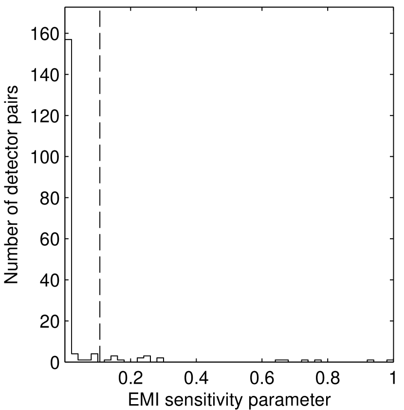
Figure 12.— EMI sensitivity parameter for all detector pairs included in Bicep2’s maps. The parameter is proportional to the contribution of possible EMI from a given detector pair to Bicep2’s polarization power spectra. The dashed line indicates the cut threshold used in constructing the EMI sensitivity pair exclusion test.

After the completion of Bicep2 observations, analysis of non-ground-subtracted galactic maps revealed clear contamination during specific temporal periods resulting from a satellite transmitter operating at the Amundsen-Scott South Pole research station. The transmitter uplink operates in the S-band (2 GHz) for approximately 7 hr per sidereal day. Details are given in Section 11.8 of the Instrument Paper.

A few factors limit the impact of electromagnetic interference (EMI) in CMB observations. One, because the satellite uplink schedule is locked to sidereal time, it so happened that the CMB field mapped by Bicep2 was always in the opposite direction from the transmitter when it was on. The opposite was true for the galactic field mapped by Bicep2. Second, a small subset of detector pairs shows much stronger differential sensitivity to the EMI than others, indicating that pair selection jackknives should fail if EMI were contributing significant power. Third, the EMI in these few pairs is visible in raw pair-difference timestreams prior to ground subtraction so that we can study its phenomenology. We find that the EMI is fixed in azimuth and constant in time, and that ground subtraction filters it nearly perfectly. The only contamination that occurs is when the transmitter turns on or off during a scanset, causing imperfect ground subtraction.

We have performed a pair exclusion test to test for EMI. Figure 12 shows an EMI sensitivity parameter for all Bicep2 detector pairs used in the final maps. The parameter is proportional to the square of the level of EMI pickup seen in non-ground-subtracted pair-difference maps of the Galactic field. The contribution of a given pair’s contamination to power spectra should thus scale with this parameter.

Because a few pairs dominate possible contamination from EMI, a pair exclusion test is more sensitive than a jackknife that splits based on the EMI statistic. We performed the test by re-coadding the real data maps and 50 signal-plus-noise simulations, excluding the 18 most sensitive pairs. The change in the resulting $BB$ bandpowers, $\Delta C_{\ell}^{BB}=C_{\ell}^{BB,\mathrm{cut}}-C_{\ell}^{BB}$, is consistent with the slightly altered noise and weighting of the new map and is statistically insignificant. In fact the first five bandpowers shift slightly up when making the cut. The $\chi$ statistic (also used in Section 10.6.1) has PTE $\simeq 0.05$. The ratio of the mean EMI sensitivity parameter with and without the pair cut implies that the cut reduces any EMI contamination that is present by $\simeq 90\%$ in the polarization power spectra. Taking this into account, we place an upper limit on contamination from EMI at $r\lesssim 1.7\times 10^{-3}$ with 95% confidence. At contamination greater than this, the pair exclusion test we performed would have a $95\%$ likelihood of producing statistically significant negative $\Delta C_{\ell}^{BB}$’s.

We also note that while the coupling of EMI is not fully known, it did not appear to involve the detector antennas, most likely coupling directly to the TES islands. The mechanism should therefore manifest differently or not at all in Bicep1, which did not use TES technology. The contaminating power will therefore not be present in a Bicep1$\times$Bicep2 cross-spectrum.

Table 4Instrumental systematics

Systematic	Characteristic $r$
Crosstalk	$\simeq 3.2\times 10^{-3}$
Beams (including gain mismatch)	$<3.0\times 10^{-3}$
EMI	$\lesssim 1.7\times 10^{-3}$
Cross polar response	$\lesssim 10^{-3}$
Eetector transfer functions	$<5.7\times 10^{-4}$
Systematic polarization angle error	$<4.0\times 10^{-4}$
Gain variation E$\rightarrow$B	$<5.3\times 10^{-5}$
Random polarization angle error	$\lesssim 5.0\times 10^{-5}$
Thermal fluctuations	$<1.2\times 10^{-5}$
Ghost beams	$\simeq 7.2\times 10^{-6}$
Scan synchronous contamination	$\lesssim 1\times 10^{-8}$
Total	$\simeq(3.2-6.5)\times 10^{-3}$

Note. — The comparable characteristic $r$ of Bicep2’s statistical uncertainty is $r=3.1\times 10^{-2}$.

10.12. Overall Achieved Systematics Level

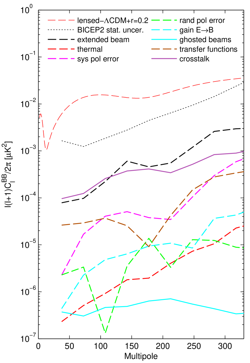
Figure 13.— Estimated levels of systematics as compared to a lensed-$\Lambda$CDM+$r=0.2$ spectrum. Solid lines indicate expected contamination. Dashed lines indicate upper limits. All systematics are comparable to or smaller than the extended beam mismatch upper limit, which is smaller than Bicep2’s statistical uncertainty.

Figure 13 shows the expected $BB$ contamination or upper limits on contamination from the individual sources of systematics considered in this section. Table 4 summarizes the $r$-values quoted for them above. To obtain a final constraint on instrumental systematics, we add the values for systematics quoted as predicted values and add the upper limits in quadrature — or the upper limit divided by two for those that are $95\%$ confidence upper limits (EMI and systematic polarization angle error). We note that magnetic pickup, which is expected to be negligible, has not been included. The total contamination and its uncertainty is almost completely dominated by the expected T$\rightarrow$P leakage from crosstalk and the uncertainty on the residual T$\rightarrow$P leakage from beam shape mismatch.

11. Conclusions

Bicep2’s systematic control demonstrates the validity of our experimental approach for high signal-to-noise CMB polarimetry. Instrumental systematics are a negligible contributor to Bicep2’s $BB$ auto spectrum. They are also small compared to Bicep2’s instrumental noise. Deprojection mitigates T$\rightarrow$P leakage from beam mismatch to a level at least sufficient to detect $r\simeq 0.003$. Other calibration measurements allow us to limit additional systematics to $r\lesssim 0.006$. For comparison, Bischoff et al. (2013) claimed a limit on instrumental systematics of $r<0.01$.

Cosmic variance limited measurements of CMB polarization promise to constrain $\Lambda$CDM cosmology with greater precision than temperature data alone (Feng et al., 2014; Galli et al., 2014). They will require control of systematics similar to Bicep2’s. Leakage from constant fractional beam mismatch (not including differential gain) scales with beam size, with leakage peaking near the beam scale. Telescopes with larger apertures than Bicep2 but similar fractional mismatch will have T$\rightarrow$P leakage that peaks at correspondingly smaller angular scales. We expect deprojection to be equally effective at filtering T$\rightarrow$P leakage at higher multipoles, as the Planck temperature maps should be sufficiently low-noise. Even if they were not, it is possible to deproject using an experiment’s own temperature map, which should always have sufficient sensitivity at the angular scales required. We do not take this approach out of simplicity to avoid complications involved with map filtering.

In summary, Bicep2’s proven systematics control demonstrates the power of scanning, small aperture, pair differencing bolometric polarimeters that do not use rotating half-wave plates or other polarization modulators. Our experimental approach will maintain its usefulness as we continue characterizing the detected $B$-mode signal.

Appendix A Parametrization of beam shapes

We define an elliptical Gaussian beam with respect to a coordinate system, $(x,y)$, that is fixed with respect to the focal plane as projected onto the sky. The parametrization of the beams is thus independent of the telescope orientation. The axes of the coordinate system are orthogonal great circles intersecting at each detector’s beam center. A detailed treatment is given in the Beams Paper. However, for the discussion below, we note that, to a very good approximation over the extent of Bicep2’s focal plane, the axes point along the rows and columns of Bicep2’s pixels.

In general, all parametrizations of elliptical Gaussians in Cartesian coordinates are of the form

$$B(\mathbf{x})=\frac{1}{\Omega}\exp\left[-(\vec{\mathbf{x}}-\vec{\boldsymbol{\mu}})^{T}\boldsymbol{\Sigma}^{-1}(\vec{\mathbf{x}}-\vec{\boldsymbol{\mu}})/2\right]$$ (A1)

where $\vec{\mathbf{x}}$ is a 2D position vector, $\vec{\boldsymbol{\mu}}$ is coordinate of the peak, $\Omega$ is a normalization constant, and $\boldsymbol{\Sigma}$ is a covariance matrix.

Differences in parametrization arise in the specification of $\boldsymbol{\Sigma}$. One common way of parametrizing an elliptical Gaussian is by specifying its major and minor widths, $\sigma_{maj}$ and $\sigma_{min}$, and the rotation $\theta$ of its major axis. In this parametrization,

$$\boldsymbol{\Sigma}=\mathbf{R}^{-1}\mathbf{C}\mathbf{R}$$ (A2)

with a covariance matrix $\mathbf{C}$ given by

$$\mathbf{C}=\left(\begin{array}[]{cc}\sigma_{maj}^{2}&0\\ 0&\sigma_{min}^{2}\end{array}\right)$$ (A3)

and a rotation matrix given by

$$\mathbf{R}=\left(\begin{array}[]{cc}\cos\theta&\sin\theta\\ -\sin\theta&\cos\theta\end{array}\right).$$ (A4)

We choose an alternate specification of the covariance matrix, given by

$$\boldsymbol{\Sigma}=\left(\begin{array}[]{cc}\sigma^{2}(1+p)&c\sigma^{2}\\ c\sigma^{2}&\sigma^{2}(1-p)\end{array}\right),$$ (A5)

where $|p|<1$, $|c|<1$, and $(p^{2}+c^{2})<1$. An elliptical Gaussian with a horizontally oriented major axis has $+p$, and an elliptical Gaussian with a vertically oriented major axis has $-p$. We refer to both as having “plus-ellipticity,” which we denote with $+$. An elliptical Gaussian with a major axis oriented $\pm 45^{\circ}$ with respect to the x-axis has $\pm c$, which we refer to as “cross-ellipticity” and denote with $\times$.

Expressed in the more familiar terms of $\sigma_{maj}$, $\sigma_{min}$ and $\theta$, we can write

$$\sigma^{2} = \left(\sigma_{maj}^{2}+\sigma_{min}^{2}\right)/2$$ (A6)

$$p = e\cos 2\theta$$ (A7)

$$c = e\sin 2\theta$$ (A8)

where we have defined the total ellipticity to be

$$e=\sqrt{p^{2}+c^{2}}=\left(\frac{\sigma_{maj}^{2}-\sigma_{min}^{2}}{\sigma_{maj}^{2}+\sigma_{min}^{2}}\right).$$ (A9)

Appendix B Heuristic description of leakage from beam mismatch

In this appendix, we discuss qualitatively how the differences of elliptical Gaussians, illustrated in Figure 2, couple to the spatial derivatives of the temperature field, $T(\mathbf{\hat{n}})$.

B.1. Gain

We model detector gain mismatch as a simple difference in normalization of circular Gaussians of nominal width given by $\delta g=g_{A}-g_{B}$ and $(g_{A}+g_{B})/2=1$. Because the difference beam, $B_{\delta g}(\mathbf{\hat{n}})$, is simply a scaled version of the nominal beam, the resulting spurious signal is a scaled version of the nominal beam-smoothed temperature, $\tilde{T}(\mathbf{\hat{n}})$ (where the tilde denotes convolution by the nominal beam). Put another way and dropping the explicit dependence on $\mathbf{\hat{n}}$, the zeroth derivative of $\tilde{T}$ multiplied by $\delta g$ is added (“leaks”) to the pair-difference timestream, $d_{T\rightarrow P}$.

B.2. Differential Pointing

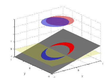
(a)

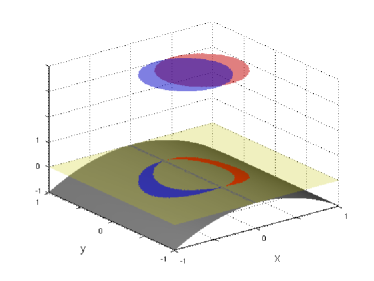
(b)

Figure 14.— Illustration of T$\rightarrow$P leakage resulting from differential pointing. The gray plane represents a $T$ sky with (a) $\nabla_{x}T>0$, $\nabla^{2}_{x}T=0$, and (b) $\nabla_{x}T=0$, $\nabla^{2}_{x}T<0$. The red and blue circles represent contour slices through the circular Gaussian beams of the A and B members of a detector pair, respectively. The non-overlapping area is projected onto the $T$ plane. The transparent green plane at $z=0$ is simply for reference. The scenario in (a) leaks T$\rightarrow$P while (b) does not.

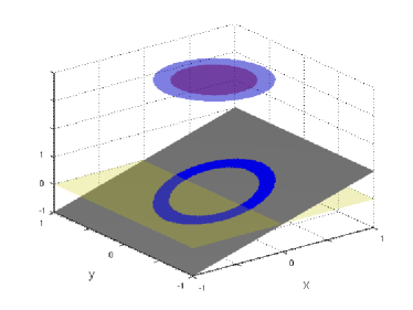
(a)

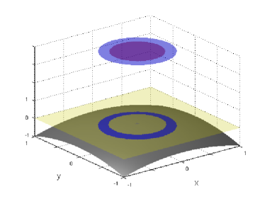
(b)

Figure 15.— Illustration of T$\rightarrow$P resulting from differential beamwidth. The gray plane represents a $T$ sky with (a) $\nabla_{x}T>0$, $\nabla^{2}_{x}T=\nabla^{2}_{y}T=0$, and (b) $\nabla_{x}T=0$, $\nabla^{2}_{x}T=\nabla^{2}_{y}T<0$. The scenario in (b) leaks T$\rightarrow$P while (a) does not.

We model differential pointing as the difference of two circular Gaussians of nominal width offset from each other in either the $x$-direction by an angular distance $\delta x=x_{A}-x_{B}$ or the $y$-direction by a distance $\delta y=y_{A}-y_{B}$. The leakage from beams offset along arbitrary directions is a linear combination of the leakage from these two orthogonal modes.

Differential pointing couples to the first derivative of $\tilde{T}$ in the direction of the pointing offset. If the first derivative of $\tilde{T}$ is zero, then regardless of where the A and B detectors are pointed, they both observe the same temperature. (If $T$ were unpolarized, the resulting pair-difference signal would be zero.) It is only if the first derivative of $\tilde{T}$ in the direction of the centroid offset is non-zero that the pair-difference timestream has contribution from $T$.

Figure 14 illustrates the coupling of differential pointing to the first derivative of $\tilde{T}$. Because, in this scenario, $\partial\tilde{T}/\partial x\equiv\nabla_{x}\tilde{T}>0$ and the centroid offset is in the $x$-direction, the A detector measures a value for temperature that is slightly larger than the value at the mean A/B beam center (pair centroid). The B detector measures a value that is slightly smaller. The pair-difference signal, A$-$B, is therefore positive. In Figure 14b, the first derivative at the pair centroid is zero while the second derivative is non-zero. In this case, both A and B measure equally negatively offset signals and the pair-difference signal is zero. Neither a non-zero first derivative in the direction perpendicular to the centroid offset nor a non-zero second derivative in any direction produces T$\rightarrow$P leakage.

An equivalent way of thinking about T$\rightarrow$P leakage resulting from beam mismatch is to describe the leaked signal as that which results from the convolution of $T$ with the difference beam, $B_{\delta}$ (Equation 6). For differential pointing the difference beam, illustrated in Figure 2, is a dipole. (Alternatively, in Figure 14, we could have shown the dipole difference beam from Figure 2 projected onto the $T$ plane.) Convolving $T$ with a dipole naturally produces a beam-smoothed map of its first derivative. (The first derivative approximation breaks down when $\delta x$ or $\delta y$ is much greater than the beamwidth.)

B.3. Beamwidth

We model differential beamwidth as the difference of two circular Gaussians with common beam centers but differing width given by $\delta\sigma=\sigma_{A}-\sigma_{B}$. Differential beamwidth couples only to the second derivatives of $T$, as illustrated in Figure 15. In Figure 15a, where the first derivative of $T$ is non-zero and the second derivative zero, neither the A nor B detector measures a signal that is offset from the value of $T$ at the pair centroid. There is no resulting T$\rightarrow$P leakage. In Figure 15b, where the first derivative of $T$ at the pair centroid is zero but the second derivatives are non-zero, both detectors measure a signal that is offset negatively. However, the B detector, which has a larger width than the A detector, measures a signal that is more negatively offset. The pair-difference signal is thus non-zero. Also apparent from Figure 15b is that a non-zero second derivative in either the $x$ or $y$ direction will produce T$\rightarrow$P leakage, which explains why the net leakage couples to the sum of the orthogonal derivatives.

B.4. Ellipticity

We model differential ellipticity as the difference of two elliptical Gaussians with either differing plus-ellipticity, given by $\delta p=p_{A}-p_{B}$, or differing cross-ellipticity, given by $\delta c=c_{A}-c_{B}$.

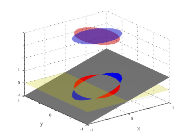
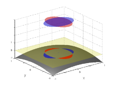
(a)	(b)
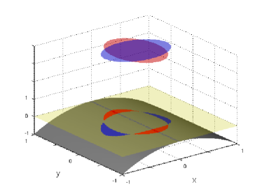
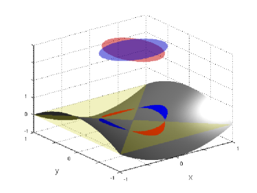
(c)	(d)
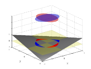
(e)

Figure 16.— Illustration of T$\rightarrow$P leakage resulting from differential plus-ellipticity. The gray plane represents a $T$ sky with (a) $\nabla_{x}T>0$, $\nabla^{2}_{x}T=\nabla^{2}_{y}T=\nabla_{x}\nabla_{y}T=0$; (b) $\nabla_{x}T=\nabla_{x}\nabla_{y}T=0$, $\nabla^{2}_{x}T=\nabla^{2}_{y}T<0$; (c) $\nabla_{x}T=\nabla_{x}\nabla_{y}T=\nabla^{2}_{y}T=0$, $\nabla^{2}_{x}T<0$; (d) $\nabla_{x}T=\nabla_{x}\nabla_{y}T=0$, $\nabla^{2}_{y}T<0<\nabla^{2}_{x}T$; (e) $\nabla_{x}T=\nabla^{2}_{x}T=\nabla^{2}_{y}T=0$, $\nabla_{x}\nabla_{y}\neq 0$. Only the scenarios in (c) and (d), which have a non-zero difference of orthogonal second derivatives, leak T$\rightarrow$P.

For differential plus-ellipticity it is only a difference in the orthogonal second derivatives of $T$ that results in T$\rightarrow$P leakage. The coupling of differential plus-ellipticity to the second derivatives of $T$ is illustrated in Figure 16. In Figure 16a, neither the A nor B detector measures a signal that is offset from the value of $T$ at the pair centroid. In Figure 16b, both detectors measure an equally negatively offset signal. In Figure 16c, both the A and B detectors measure a negatively offset signal, but the B detector measures a more negatively offset signal, and the resulting pair-difference is non-zero. In Figure 16d, the A detector measures a negatively offset signal and the B detector measures a positively offset signal, and the resulting pair-difference is also non-zero. In Figure 16e, which has zero first and second derivatives at the pair centroid but a non-zero cross derivative, neither detector measures an offset signal, and the pair-difference is zero.

A figure depicting differential cross-ellipticity analogous to Figure 16 is not shown. It would be identical to Figure 16 with the beams (or $T$) rotated by $45^{\circ}$. After doing this, only Figure 16e, which has a non-zero cross-derivative, would leak T$\rightarrow$P. Thus for differential cross-ellipticity, only a non-zero cross-derivative of $T$ produces T$\rightarrow$P leakage.

B.5. Crosstalk and Ghost Beams

Non-main-beam systematics can also be described by mismatches of elliptical Gaussians. Crosstalk and internal reflections in the optics produce secondary beams of smaller amplitude offset from the main beam. Again, it is only an A/B mismatch of these secondary beams that results in T$\rightarrow$P leakage. The secondary beams can, in general, exhibit their own mismatch, independent of the main beam mismatch. They couple to the derivatives of $T$ not at the main beam centroid but at their own centroid. The leakage is still entirely deterministic and analyzable in terms of mismatched elliptical Gaussians.

Appendix C Mathematical Description of Deprojection

This section formally derives the leakage templates and fit coefficients listed in Table 3. A similar description of this formalism is given in Aikin 2013.

In all cases other than differential gain, we proceed by Taylor expanding an elliptical Gaussian about the differential parameter, then expressing the difference of perturbed beams as a linear combination of spatial derivatives of the nominal Gaussian beam. We then express the leaked signal as the convolution of the temperature field with the Taylor expanded difference beam.

C.1. Differential Gain

We start by again noting that the T$\rightarrow$P leakage from beam mismatch is simply $T$ convolved with a detector pair’s $A-B$ difference beam, $B_{\delta}$, as expressed in Equation 6, and where we have dropped the explicit dependence on $\mathbf{\hat{n}}$.

A gain mismatch between two Gaussian beams is parametrized as a difference in the peak heights of the A and B beams,

$$B_{\delta g}(r) = B_{A}(r)-B_{B}(r)$$ (C1)

$$= \frac{g_{A}}{2\pi\sigma^{2}}\exp(-r^{2}/2\sigma^{2})-\frac{g_{B}}{2\pi\sigma^{2}}\exp(-r^{2}/2\sigma^{2})$$

$$= \delta g\frac{\exp(-r^{2}/2\sigma^{2})}{2\pi\sigma^{2}}$$

$$= \delta gB(r)$$

where $\delta g=g_{A}-g_{B}$ and $B(r)$ without a subscript denotes the nominal, un-differenced, circular Gaussian beam, and is a function of 1-dimensional radius $r$ instead of a 2D position vector $\mathbf{n}$. Note that here, the gain $g$ is defined so that the mean gain, $(g_{A}+g_{B})/2=1$. The resulting leaked signal is

$$d_{\delta g} = T\ast B_{\delta g}(r)$$ (C2)

$$= \delta g\tilde{T}$$

where $\tilde{T}=T\ast B(r)$ is just $T$ convolved with the nominal, circular Gaussian beam.

As discussed in Section 5.2, the method of deprojecting gain mismatch is then as follows: first, in the map making stage, after computing the R.A./decl. trajectories of detector pairs, we create a leakage template timestream, $\tilde{T}(t)$, for each detector pair by sampling a Healpix temperature map along the pair’s trajectory. (The Healpix map is pre-smoothed to Bicep2’s nominal circular Gaussian beam.) Second, we filter $\tilde{T}(t)$ exactly as is done to the real data timestreams. Lastly, we regress the pair-difference data against $\tilde{T}(t)$ and subtract the best-fit template. The fit coefficient is proportional to $\delta g$. Alternately, if we know each detector pair’s differential gain a priori, we can simply scale and subtract the template.

C.2. Differential Pointing

To describe a Gaussian whose centroid is displaced in the focal plane $x$-direction by a small fraction of the beamwidth, we express the nominal circular Gaussian beam $B(r)$ in terms of $x$ and $y$ and Taylor expand about $x$, so that

$$B(x+\delta x,y) = B(x,y)+\left.\frac{\partial B(x^{\prime},y)}{\partial x^{\prime}}\right|_{x}\delta x+$$ (C3)

$$\left.\frac{1}{2}\frac{\partial^{2}B(x^{\prime},y)}{\partial x^{\prime 2}}\right|_{x}(\delta x)^{2}+...$$

where $\delta x$ is the displacement in $x$ and, as before,

$$B(x,y)=B(r)=\exp[-(x^{2}+y^{2})/2\sigma^{2}]/2\pi\sigma^{2}$$ (C4)

is the unperturbed, un-differenced, circular Gaussian beam. Then, calculating the difference beam that results from displacing the A beam by $+\delta x/2$ and the B beam by $-\delta x/2$ (and noting that the first and third terms in Equation C3, and indeed any term that is an even power of $\delta x$, cancel),

$$B_{\delta x}(x,y) = B(x+\delta x/2,y)-B(x-\delta x/2,y)$$ (C5)

$$= \left.\frac{\partial B(x^{\prime},y)}{\partial x^{\prime}}\right|_{x}\delta x+\mathcal{O}[(\delta x)^{3}]$$

$$\simeq \delta x\nabla_{x}B(x,y),$$

where we have defined the partial derivative with respect to focal plane coordinate $x$

$$\nabla_{x}\equiv\frac{\partial}{\partial x}.$$ (C6)

The leaked signal resulting from differential pointing in the focal plane $x$-direction is then

$$d_{\delta x} = T\ast B_{\delta x}$$ (C7)

$$\simeq \delta x(T\ast\nabla_{x}B)$$

$$= \delta x\nabla_{x}(T\ast B)$$

$$= \delta x\nabla_{x}\tilde{T}.$$

Similarly, for a pointing displacement in the focal plane $y$-direction, the leaked signal is

$$d_{\delta y}=\delta y\nabla_{y}\tilde{T}.$$ (C8)

A differential pointing offset in any arbitrary direction can be expressed as the linear combination of equations C7 and C8. These equations then tell us how to construct the leakage templates for differential pointing. Synfast can produce sky maps of the first derivatives of the circular Gaussian-smoothed temperature map expressed in the Healpix latitude/longitude coordinate system, $\nabla_{\theta}\tilde{T}(\mathbf{\hat{n}})$ and $\nabla_{\phi}\tilde{T}(\mathbf{\hat{n}})$. We sample the Gaussian-smoothed derivative maps along a detector pair’s pointing trajectory as a function of time to create two template timestreams, $\nabla_{\theta}\tilde{T}(t)$ and $\nabla_{\phi}\tilde{T}(t)$. Then, knowing the focal plane’s orientation on the sky at each point in the timestream, we apply the chain rule for derivatives to transform the derivative timestreams from the Healpix coordinate system to the focal plane $(x,y)$ coordinate system.

Once $\nabla_{x}\tilde{T}(t)$ and $\nabla_{y}\tilde{T}(t)$ have been constructed and filtered like the real data, they are simultaneously fit to the pair-difference data. The fit coefficients are $\delta x$ and $\delta y$.

C.3. Differential Beamwidth

The derivation of the templates for differential beamwidth (and differential ellipticity) proceeds similarly to that for differential pointing. Taylor expanding the nominal beam about the parameter to be perturbed, in this case $\sigma$, we have

$$B(x,y,\sigma+\delta\sigma) = B(x,y,\sigma)+\left.\frac{\partial B(x,y,\sigma^{\prime})}{\partial\sigma^{\prime}}\right|_{\sigma}\delta\sigma$$ (C9)

$$+\left.\frac{1}{2}\frac{\partial^{2}B(x,y,\sigma^{\prime})}{\partial\sigma^{\prime 2}}\right|_{\sigma}(\delta\sigma)^{2}+...$$

Again noting that even powers of $\delta\sigma$ cancel, the difference beam is

$$B_{\delta\sigma}(x,y) = B(x,y,\sigma+\delta\sigma/2)-B(x,y,\sigma-\delta\sigma/2)$$ (C10)

$$\simeq \left.\frac{\partial B(x,y,\sigma^{\prime})}{\partial\sigma^{\prime}}\right|_{\sigma}\delta\sigma+\mathcal{O}[(\delta\sigma)^{3}].$$

One can write

$$\frac{\partial B(x,y,\sigma)}{\partial\sigma}=\left(\frac{x^{2}+y^{2}}{\sigma^{3}}-\frac{2}{\sigma}\right)B(x,y,\sigma).$$ (C11)

One can also can write

$$\nabla^{2}_{x}B(x,y) = \left(\frac{x^{2}}{\sigma^{4}}-\frac{1}{\sigma^{2}}\right)B(x,y)$$ (C12)

$$\nabla^{2}_{y}B(x,y) = \left(\frac{y^{2}}{\sigma^{4}}-\frac{1}{\sigma^{2}}\right)B(x,y)$$ (C13)

$$(\nabla^{2}_{x}+\nabla^{2}_{y})B(x,y) = \left(\frac{x^{2}+y^{2}}{\sigma^{2}}-2\right)\frac{B(x,y)}{\sigma^{2}}$$ (C14)

where we have defined the second partial derivatives with respect to focal plane coordinates $x$ and $y$

$$\nabla^{2}_{x}\equiv\frac{\partial^{2}}{\partial x^{2}},\nabla^{2}_{y}\equiv\frac{\partial^{2}}{\partial y^{2}}.$$ (C15)

Equation C11 can then be written as

$$\frac{\partial B(x,y,\sigma)}{\partial\sigma}=\sigma(\nabla^{2}_{x}+\nabla^{2}_{y})B(x,y)$$ (C16)

and Equation C10 becomes

$$B_{\delta\sigma}\simeq\sigma\delta\sigma(\nabla^{2}_{x}+\nabla^{2}_{y})B(x,y)$$ (C17)

The T$\rightarrow$P leakage from differential beamwidth is then

$$d_{\delta\sigma} = B_{\delta\sigma}\ast T$$ (C18)

$$\simeq \sigma\delta\sigma(\nabla^{2}_{x}+\nabla^{2}_{y})B\ast T$$

$$\simeq \sigma\delta\sigma(\nabla^{2}_{x}+\nabla^{2}_{y})\tilde{T}.$$

Because differential beamwidth is monopole symmetric, only one template needs to be constructed for deprojection. To construct the template, we sample $\nabla_{\theta\theta}\tilde{T}(\mathbf{\hat{n}})$, $\nabla_{\phi\phi}\tilde{T}(\mathbf{\hat{n}})$ and $\nabla_{\theta\phi}\tilde{T}(\mathbf{\hat{n}})$ along each detector pair’s pointing trajectory, apply the chain rule for derivatives to construct $\nabla^{2}_{x}\tilde{T}(t)$ and $\nabla^{2}_{y}\tilde{T}(t)$ (though the monopole symmetry makes this step unnecessary), add them together, filter the sum like the real data, and fit the resulting template to the pair-difference timestream. The fit coefficient is $\sigma\delta\sigma$.

C.4. Differential Ellipticity

The difference beam corresponding to mismatched beam ellipticity is a quadrupole. The orientation of the quadrupole is arbitrary, but can be approximated as the linear combination of two orthogonal quadrupoles, chosen as the plus and cross orientations.

An elliptical Gaussian with pure plus-ellipticity is written as

$$B(x,y,p)=\frac{1}{2\pi\sigma^{2}}\exp\left[-\frac{1}{2\sigma^{2}}\left(\frac{x^{2}}{1+p}+\frac{y^{2}}{1-p}\right)\right].$$ (C19)

Taylor expanding the plus-ellipticity beam about $p=0$ yields

$$B(x,y,p)\simeq B(p=0)+\left.\frac{\partial B(x,y,p^{\prime})}{\partial p^{\prime}}\right|_{0}p+\frac{1}{2}\left.\frac{\partial^{2}B(x,y,p^{\prime})}{\partial p^{\prime 2}}\right|_{0}p^{2}+...~{}.$$ (C20)

Then, noting that we can write

$$\left.\frac{\partial B(x,y,p^{\prime})}{\partial p^{\prime}}\right|_{0}=\left(\frac{x^{2}-y^{2}}{2\sigma^{2}}\right)B(x,y),$$ (C21)

where again, $B(x,y)=B(x,y,p=0)$ is the nominal, circular Gaussian beam, and using Equations C12 and C13 to write

$$(\nabla^{2}_{x}-\nabla^{2}_{y})B(x,y)=\left(\frac{x^{2}-y^{2}}{\sigma^{4}}\right)B(x,y)$$ (C22)

the difference beam is

$$B_{\delta p}(x,y) = B(x,y,p_{A})-B(x,y,p_{B})$$ (C23)

$$= \delta p\left(\frac{x^{2}-y^{2}}{2\sigma^{2}}\right)B(x,y)+\mathcal{O}(p_{A}^{2}-p_{B}^{2})+...$$

$$\simeq \frac{\sigma^{2}}{2}\delta p(\nabla^{2}_{x}-\nabla^{2}_{y})B(x,y),$$

where $\delta p=p_{A}-p_{B}$. Note that the ellipticity difference beam is accurate only to first order rather than second order like the other Gaussian modes. Also note that the difference beam is accurate to order $p_{A}^{2}-p_{B}^{2}$ rather than $(\delta p)^{2}$. Thus, large enough ellipticities can cause a breakdown of deprojection even if the differential ellipticity is small. The T$\rightarrow$P leakage resulting from differential plus-ellipticity is

$$d_{\delta p} = B_{\delta p}\ast T$$ (C24)

$$\simeq \frac{\sigma^{2}}{2}\delta p(\nabla^{2}_{x}-\nabla^{2}_{y})\tilde{T}.$$

Now we consider cross-ellipticity. An elliptical Gaussian with pure cross-ellipticity can be written as

$$B(x,y,c)=\frac{1}{2\pi\sigma^{2}}\exp\left[-\frac{1}{2(1-c^{2})\sigma^{2}}(x^{2}+y^{2}-2cxy)\right],$$ (C25)

We work to linear order in $c$ and set $(1-c^{2})\simeq 1$. Proceeding as above, and noting that

$$\nabla_{x}\nabla_{y}B(x,y)=\frac{1}{\sigma^{4}}xyB(x,y),$$ (C26)

where we have defined the cross-derivative with respect to focal plane coordinates

$$\nabla_{x}\nabla_{y}\equiv\frac{\partial^{2}}{\partial x\partial y},$$ (C27)

we can write

$$\left.\frac{\partial B(x,y,c^{\prime})}{\partial c^{\prime}}\right|_{0} = \frac{1}{\sigma^{2}}xyB(x,y)$$ (C28)

$$= \sigma^{2}\nabla_{x}\nabla_{y}B(x,y).$$

The difference beam resulting from differential cross-ellipticity is then

$$B_{\delta c} = B(x,y,c_{A})-B(x,y,c_{B})$$ (C29)

$$= \sigma^{2}\delta c\nabla_{x}\nabla_{y}B(x,y)+\mathcal{O}(c_{A}^{2}-c_{B}^{2})+...~{}.$$

where $\delta c=c_{A}-c_{B}$. The T$\rightarrow$P leakage resulting from differential cross-ellipticity is

$$d_{\delta c}\simeq\sigma^{2}\delta c\nabla_{x}\nabla_{y}\tilde{T}.$$ (C30)

C.5. Practical Implementation

In the map making stage, we construct deprojection template timestreams for each detector pair in the same manner as we construct simulated timestreams — by interpolating off a suitably pre-smoothed deprojection template map along the pointing trajectory of a detector pair’s mean centroid. The deprojection template maps are simply a $T$ map and its first, second, and cross-derivatives, all smoothed by Bicep2’s measured mean, azimuthally averaged beam profile.

We interpolate off the deprojection $T$ map using the first and second derivative $T$ maps to perform a second order Taylor expansion around the nearest neighbor pixel center. This is identical to the interpolation used in the forward simulation pipeline. We interpolate off the first derivative maps using the second derivative maps to perform a first order Taylor expansion around the nearest neighbor pixel centers. We interpolate off the second derivative maps using nearest neighbor interpolation, which we find to have adequate accuracy for deprojection.

The interpolation scheme introduces the possibility that certain simulations of beam mismatch might be deprojected to artificially high accuracy and indeed we can simulate differential pointing in such a way that it deprojects to numerical precision. However, this is not an issue in practice as (i) we perform simulations with an Nside=2048 input map but use an Nside=512 map for deprojection, (ii) noise in the template map, which we account for, sets the primary limitation on deprojection, (iii) our multiple Gaussian convolution scheme simulates differential beamwidth and ellipticity with higher accuracy than the leakage templates and, most importantly, (iv) the special beam map simulations on which we ultimately rely to characterize residual contamination from beam mismatch after deprojection do not use the same interpolation scheme as the computation of the leakage template timestreams at all.

The template map used for deprojection of the main results is the Planck HFI 143 GHz map, re-smoothed to Bicep2’s measured mean beam profile and downgraded to Nside=512. We do not use derived data products meant to contain only CMB with no foregrounds (i.e. SMICA) because Bicep2’s T$\rightarrow$P leakage does, in principle, include foreground $T$ at some very low level and we expect the Planck 143 GHz bandpass to most closely match Bicep2’s. We smooth the Planck map to match Bicep2’s beamwidth by computing the Planck map’s $a_{\ell m}$s using anafast and multiplying them by the ratio of Bicep2’s mean azimuthally symmetric beam window function (as measured from beam maps) to Planck’s published 143 GHz beam window function, $B_{\ell}^{B2}/B_{\ell}^{Pl}$, as presented in Planck Collaboration et al. (2014a). We then convert back to map space with synfast.

We simulate template map noise by using publicly available Planck noise maps to generate simulated realizations of uncorrelated, white noise temperature maps. We then apply the same resmoothing procedure to the noise realizations as the real template map (convert to $a_{\ell m}$s and multiply by $B_{\ell}^{B2}/B_{\ell}^{Pl}$), and use synfast to produce derivatives of the noise realizations. We add these noise realizations to noiseless simulated maps containing lensed-$\Lambda$CDM signal. We use the same procedure to simulate WMAP template map noise.

In general, prior to fitting, the leakage template timestreams must be subjected to any filtering or manipulation beyond pair differencing to which the data timestreams themselves are subjected. For Bicep2 this involves third-order polynomial filtering of half scans and ground subtraction.

At this point, we could fit the deprojection templates directly to the timestreams. However, because we co-add the data from each detector pair into intermediate maps (the “pair maps” described in §IV.D of the Results Paper) on approximately one hour timescales (a “scanset”) we choose to bin the deprojection template timestreams into map pixels on the same timescale. When coadding the pair maps into final $T$, $Q$ and $U$ maps, we can choose the timescale in multiples of one hour over which to co-add the leakage templates prior to performing deprojection.

As discussed, deprojection, like all filtering operations, removes information and produces some amount of E$\rightarrow$B mixing. In general, this mixing and mode removal becomes worse when coadding the templates over shorter durations due to the decreased coverage of the intermediate map, which results in more degrees of freedom being removed from the final map. While coadding over all three years of Bicep2 data would produce the minimum possible mode removal, because the telescope scan pattern repeats every 72 hr, coadding over timescales longer than this makes no practical difference. Coadding over shorter timescales allows time variable systematics to be filtered out. We fully expect beam shape mismatch to remain constant in time, but, as discussed in Section 10.3, gain mismatch could presumably have a time variable component. We therefore choose to co-add the data and deprojection templates over approximately 9 hr timescales (1 “phase,” equivalent to 10 scansets) prior to performing deprojection. Using the matrix purification power spectrum estimator discussed in §VI.B of the Results Paper, we find that this does not significantly increase the uncertainty of our final bandpowers. In any case, the E$\rightarrow$B leakage and mode removal caused by deprojection is the same as that from any filtering operation and is fully captured by our simulation-based analysis.

Appendix D Beam map simulation uncertainty

We estimate the uncertainty of the contamination predicted from beam map simulations and shown in Figures 11 and 13 using a standard resampling method known as a delete-one jackknife, not to be confused with the jackknife tests described in Section 8 and throughout the paper. The method is as follows: the composite beam maps described in Section 10.1 are the mean of 12 independent measurements. (For the extended composite beam, they are the median of the measurements.) We remake the composite beam maps 12 times, excluding in turn 1 of the 12 measurements prior to taking the mean. This generates 12 additional sets of simulated spectra. The standard deviation of the 12 bandpowers in each $\ell$ bin, multiplied by $\sqrt{N-1}$, where $N=12$ is the number of independent measurements, provides an estimate of the standard error in each bin. The difference of the mean of the 12 bandpowers and the bandpower from the main simulation, multiplied by $(N-1)$, provides an estimate of the bias in each bin. The bias and standard error of the predicted contamination from beam mismatch at $r<1.2^{\circ}$ is robust because the beam maps are mean filtered in this region and because each beam map pixel is covered by all 12 observations. (For the extended beam map an effective number of observations, $N_{eff}<12$, must be used.)

We apply identical differential gain normalization to the composite beam maps in each of the $12$ delete-one jackknife realizations. Uncertanties in the differential gain measurements are therefore not accounted for. From the standard deviation of these measurements made from different temporal subsets of Bicep2 data, and from simulations that include the effect of $\Lambda$CDM $TE$ correlation in our absolute calibration procedure, we estimate that their uncertainty is $\sigma_{\delta g}\simeq 0.02$. We perform noiseless, temperature-only simulations using the Planck 143 GHz map as an input to the standard simulation pipeline described in Section 7.1. In each multipole bin, we compute the standard deviation of $50$ realizations of a random 2% gain mismatch ($\overline{\delta g}=0$, $\langle\delta g^{2}\rangle^{1/2}=0.02$) and add this to the uncertainties predicted from the delete-one jackknife. (The sum as opposed to the quadrature sum is appropriate for bandpowers.)

We make a correction to the simulated main beam leakage spectra by subtracting the predicted bias, which is $\sim 3-10\times$ smaller than the simulated leakage after deprojection. The corrected leakage, shown in Figure 11, is statistically significant compared to its estimated uncertainty. The extended beam maps are observed with less redundancy and are thus noisier than the main beam maps. The bias corrected leakage from the extended beam simulations is consistent with zero. Its estimated uncertainty is plotted as the “extended beams” line in Figure 13.

References

- Abbott & Wise (1984) Abbott, L. F., & Wise, M. B. 1984, Nuclear Physics B, 244, 541
- Aikin (2013) Aikin, R. W. 2013, PhD thesis, California Institute of Technology
- Barkats et al. (2014) Barkats, D., Aikin, R., Bischoff, C., et al. 2014, Astrophys. J. , 783, 67
- Bicep2 and Keck Array Collaborations IV (2015) Bicep2 and Keck Array Collaborations IV. 2015, Astrophys. J. , 806, 206
- Bicep2 and Keck Array Collaborations V (2015) Bicep2 and Keck Array Collaborations V. 2015, Astrophys. J. , 811, 126
- Bicep2 Collaboration et al. (2015) Bicep2 Collaboration, Keck Array Collaboration, SPIDER Collaboration, et al. 2015, Astrophys. J. , 812, 176
- Bicep2 Collaboration I (2014) Bicep2 Collaboration I. 2014, Phys. Rev. Lett., 112, 241101
- Bicep2 Collaboration II (2014) Bicep2 Collaboration II. 2014, The Astrophysical Journal, 792, 62
- Bierman et al. (2011) Bierman, E. M., Matsumura, T., Dowell, C. D., et al. 2011, Astrophys. J. , 741, 81
- Bischoff et al. (2013) Bischoff, C., Brizius, A., Buder, I., et al. 2013, Astrophys. J. , 768, 9
- Bond & Efstathiou (1984) Bond, J. R., & Efstathiou, G. 1984, Astrophys. J. Lett. , 285, L45
- Brevik (2012) Brevik, J. A. 2012, PhD thesis, California Institude of Technology
- Chiang et al. (2010) Chiang, H. C., Ade, P. A. R., Barkats, D., et al. 2010, Astrophys. J. , 711, 1123
- Crites et al. (2014) Crites, A. T., Henning, J. W., Ade, P. A. R., et al. 2014, ArXiv e-prints, arXiv:1411.1042
- Das et al. (2014) Das, S., Louis, T., Nolta, M. R., et al. 2014, JCAP , 4, 14
- de Korte et al. (2003) de Korte, P. A. J., Beyer, J., Deiker, S., et al. 2003, Review of Scientific Instruments, 74, 3807
- Fabbri & Pollock (1983) Fabbri, R., & Pollock, M. D. 1983, Physics Letters B, 125, 445
- Feng et al. (2014) Feng, J. L., Ritz, S., Beatty, J. J., et al. 2014, ArXiv e-prints, arXiv:1401.6085
- Fowler et al. (2010) Fowler, J. W., Acquaviva, V., Ade, P. A. R., et al. 2010, Astrophys. J. , 722, 1148
- Galli et al. (2014) Galli, S., Benabed, K., Bouchet, F., et al. 2014, Phys. Rev. D , 90, 063504
- Grishchuk (1975) Grishchuk, L. P. 1975, Soviet Journal of Experimental and Theoretical Physics, 40, 409
- Hinshaw et al. (2013) Hinshaw, G., Larson, D., Komatsu, E., et al. 2013, Astrophys. J. Suppl. , 208, 19
- Hivon et al. (2002) Hivon, E., Górski, K. M., Netterfield, C. B., et al. 2002, Astrophys. J. , 567, 2
- Hou et al. (2014) Hou, Z., Reichardt, C. L., Story, K. T., et al. 2014, Astrophys. J. , 782, 74
- Hu et al. (2003) Hu, W., Hedman, M. M., & Zaldarriaga, M. 2003, Phys. Rev. D , 67, 043004
- Irwin et al. (2002) Irwin, K. D., Vale, L. R., Bergren, N. E., et al. 2002, Low Temperature Detectors, 605, 301
- Jarosik et al. (2011) Jarosik, N., Bennett, C. L., Dunkley, J., et al. 2011, Astrophys. J. Suppl. , 192, 14
- Kamionkowski et al. (1997) Kamionkowski, M., Kosowsky, A., & Stebbins, A. 1997, Phys. Rev. Lett., 78, 2058
- Kaufman (2014) Kaufman, J. P. 2014, PhD thesis, University of California, San Diego
- Keating et al. (2013) Keating, B. G., Shimon, M., & Yadav, A. P. S. 2013, Astrophys. J. Lett. , 762, L23
- Kernasovskiy et al. (2012) Kernasovskiy, S., Ade, P. A. R., Aikin, R. W., et al. 2012, in Society of Photo-Optical Instrumentation Engineers (SPIE) Conference Series, Vol. 8452, Society of Photo-Optical Instrumentation Engineers (SPIE) Conference Series, 84521B
- Kovac et al. (2002) Kovac, J. M., Leitch, E. M., Pryke, C., et al. 2002, Nature, 420, 772
- Kuo et al. (2008) Kuo, C. L., Bock, J. J., Bonetti, J. A., et al. 2008, in Society of Photo-Optical Instrumentation Engineers (SPIE) Conference Series, Vol. 7020, Society of Photo-Optical Instrumentation Engineers (SPIE) Conference Series, 70201I
- Lueker et al. (2010) Lueker, M., Reichardt, C. L., Schaffer, K. K., et al. 2010, Astrophys. J. , 719, 1045
- Naess et al. (2014) Naess, S., Hasselfield, M., McMahon, J., et al. 2014, JCAP , 10, 7
- O’Brient et al. (2012) O’Brient, R., Ade, P. A. R., Ahmed, Z., et al. 2012, in Society of Photo-Optical Instrumentation Engineers (SPIE) Conference Series, Vol. 8452, Society of Photo-Optical Instrumentation Engineers (SPIE) Conference Series, 84521G
- O’Dea et al. (2007) O’Dea, D., Challinor, A., & Johnson, B. R. 2007, Mon. Not. Roy. Astron. Soc. , 376, 1767
- Penzias & Wilson (1965) Penzias, A. A., & Wilson, R. W. 1965, Astrophys. J. , 142, 419
- Planck Collaboration et al. (2014a) Planck Collaboration, Ade, P. A. R., Aghanim, N., et al. 2014a, Astr. & Astroph. , 571, A7
- Planck Collaboration et al. (2014b) —. 2014b, Astr. & Astroph. , 571, A8
- Planck Collaboration et al. (2014c) —. 2014c, Astr. & Astroph. , 571, A16
- Polnarev (1985) Polnarev, A. G. 1985, Sov. Ast. , 29, 607
- Pryke et al. (2009) Pryke, C., Ade, P., Bock, J., et al. 2009, Astrophys. J. , 692, 1247
- QUIET Collaboration et al. (2011) QUIET Collaboration, Bischoff, C., Brizius, A., et al. 2011, Astrophys. J. , 741, 111
- QUIET Collaboration et al. (2012) QUIET Collaboration, Araujo, D., Bischoff, C., et al. 2012, Astrophys. J. , 760, 145
- Rubakov et al. (1982) Rubakov, V. A., Sazhin, M. V., & Veryaskin, A. V. 1982, Physics Letters B, 115, 189
- Seljak (1997) Seljak, U. 1997, Astrophys. J. , 482, 6
- Seljak & Zaldarriaga (1997) Seljak, U., & Zaldarriaga, M. 1997, Phys. Rev. Lett., 78, 2054
- Sheehy (2013) Sheehy, C. D. 2013, PhD thesis, University of Chicago
- Sheehy et al. (2010) Sheehy, C. D., Ade, P. A. R., Aikin, R. W., et al. 2010, Proc. SPIE, 7741, 77411R
- Shimon et al. (2008) Shimon, M., Keating, B., Ponthieu, N., & Hivon, E. 2008, Phys. Rev. D , 77, 083003
- Sievers et al. (2013) Sievers, J. L., Hlozek, R. A., Nolta, M. R., et al. 2013, Journal of Cosmology and Astroparticle Physics, 10, 60
- Starobinsky (1979) Starobinsky, A. A. 1979, Soviet Journal of Experimental and Theoretical Physics Letters, 30, 682
- Story et al. (2013) Story, K. T., Reichardt, C. L., Hou, Z., et al. 2013, Astrophys. J. , 779, 86
- Takahashi et al. (2010) Takahashi, Y. D., Ade, P. A. R., Barkats, D., et al. 2010, Astrophys. J. , 711, 1141
- Wandelt & Górski (2001) Wandelt, B. D., & Górski, K. M. 2001, Phys. Rev. D , 63, 123002
- Yoon et al. (2006) Yoon, K. W., et al. 2006, in Presented at the Society of Photo-Optical Instrumentation Engineers (SPIE) Conference, Vol. 6275, Society of Photo-Optical Instrumentation Engineers (SPIE) Conference Series, 62751K