A Class of DCT Approximations Based on the Feig-Winograd Algorithm

Abstract

A new class of matrices based on a parametrization of the Feig-Winograd factorization of $8$-point DCT is proposed. Such parametrization induces a matrix subspace, which unifies a number of existing methods for DCT approximation. By solving a comprehensive multicriteria optimization problem, we identified several new DCT approximations. Obtained solutions were sought to possess the following properties: (i) low multiplierless computational complexity, (ii) orthogonality or near orthogonality, (iii) low complexity invertibility, and (iv) close proximity and performance to the exact DCT. Proposed approximations were submitted to assessment in terms of proximity to the DCT, coding performance, and suitability for image compression. Considering Pareto efficiency, particular new proposed approximations could outperform various existing methods archived in literature.

Keywords
DCT approximation, Feig-Winograd algorithm, Low-complexity transforms, Image compression

1 Introduction

The discrete cosine transform (DCT) is an essential tool in digital signal processing [1, 2]. This is mainly because the DCT is asymptotically equivalent to the Karhunen-Loève transform (KLT), which possesses optimal decorrelation and energy compaction properties [3, 4, 1, 2, 5, 6]. Such good characteristics are attained when high correlated first-order Markov signals are considered [1, 2]. Importantly natural images belong to this particular class of signals [5].

In particular, the DCT has been adopted in several image and video coding schemes [7], such as JPEG [8], MPEG-1 [9], MPEG-2 [10], H.261 [11], H.263 [12], ACV/H.264 [13], and the recent HEVC/H.265 [14]. In particular, H.264 and HEVC standards employ 8-point DCT algorithms [15, 16, 17, 18, 19, 14, 20, 21] among other different blocklenghts, such as 4, 16, and 32 points [22, 23]. In [24], the 8-point DCT stage of the HEVC was optimized. Because of this increasing demand, several algorithms for the efficient computation of the 8-point DCT have been proposed [25, 26]. In [1, 2], comprehensive surveys on DCT algorithms are detailed.

Noteworthy DCT methods include the following procedures: Wang factorization [27], Lee DCT for power-of-two block lengths [28], Arai DCT scheme [29], Loeffler algorithm [30], and Feig-Winograd factorization [31]. All these algorithms are classical results in the field and have been considered for practical applications [9, 32, 33]. For instance, the Arai DCT scheme was employed in various recent hardware implementations of the DCT [34, 35, 36].

Indeed, after the introduction of the DCT by Ahmed et al. [3] in 1974, designing efficient DCT algorithms has been a major scientific effort in the circuits, systems, and signal processing community. Because of such intense research in the field, the current exact methods are very close to the theoretical DCT complexity [5, 37, 38, 30, 29]. Therefore, it may be unrealistic to expect that new exact algorithms could offer dramatic computational gains for such a fundamental and deeply investigated mathematical operation.

In this scenario, approximate methods offer an alternative way to further reduce the computational complexity of the DCT [2, 6, 39, 40, 41, 42]. While not computing the DCT exactly, such approximations can provide meaningful estimations at very low-complexity computational requirements. In this sense, literature has been populated with approximate methods for the efficient computation of the DCT. For example, the AVC/H.264 and HEVC/H.265 standards employ integer approximate DCT in order to reduce the computational cost of the transform stage. A comprehensive list of approximate methods for the DCT is found in [2]. Prominent methods include the signed DCT (SDCT) [6], the level 1 approximation by Lengwehasatit-Ortega [43], the Bouguezel-Ahmad-Swamy (BAS) series of algorithms [41, 44, 45, 46, 42, 47], the DCT round-off approximation [48], the modified DCT round-off approximation [40], and the multiplier-free DCT approximation for radio-frequency (RF) multi-beam digital aperture-array space imaging [49].

Although several other types of approximations are available, in general, very low-complexity approximation matrices have their elements defined on the set $\{0,\pm 1/2,\pm 1,\pm 2\}$ [40, 48, 6, 42, 47]. Thus, such transformations possess null multiplicative complexity, because the required arithmetic operations can be implemented exclusively by means of binary additions and bit-shifting operations. Indeed, DCT approximations can replace the exact DCT in hardware implementation and high-speed computation/processing [2], while having low hardware costs and low power demands [36]. Effectively, DCT approximations have been considered for applications in real-time video transmission and processing [50, 51], satellite communication systems [2], portable computing applications [2], radio-frequency smart antenna array [49], and wireless image sensor networks [52].

The proposed methods archived in literature for generating very low complexity approximations include: (i) crude approximations [6, 48, 47]; (ii) inspection [41, 45, 46]; (iii) variations of previous approximations via a single-parameter matrix [42]; and (iv) optimization procedures based on the DCT structure [49]. Thus, the existing approximations appear as isolate cases without a unifying mathematical formalism.

The aim of this paper is two-fold. Our first goal is to introduce a new class of DCT approximations. For such end, we consider a parametrization of the Feig-Winograd factorization of the 8-point DCT matrix [31]. Such parametrization allows the constructions of a specific matrix subspace. Second, over the introduced subspace, we solve a constrained multicriteria optimization problem to identifying optimal DCT approximations according to several figures of merit for image compression. Both orthogonal and non-orthogonal approximations are sought.

The paper unfolds as follows. In Section 2, we describe the mathematical structure of the proposed class of transforms, including fast algorithms for the direct and inverse transformations. Section 3 discusses the desirable properties that approximate $8$-point DCTs are expected to satisfy, such as low computational complexity, orthogonality, invertibility, and proximity to the exact DCT. In Section 4, we formalize a multicriteria optimization problem based on a comprehensive set of performance measures in order to identify efficient solutions and new transformations over the proposed class of matrices. The resulting approximations are subject to assessment and extensive comparison with competing methods. In Section 5, we perform a comprehensive image compression analysis considering the obtained optimal transforms. using image quality measures as figures of merit. Section 6 concludes the paper.

2 Feig-Winograd Approximate DCT

2.1 Preliminaries

The DCT is algebraically represented by the $N\times N$ transformation matrix $\mathbf{C}_{N}$ whose elements are given by [1, 2]:

$$c_{m,n}=\sqrt{\frac{2}{N}}\,\beta_{m-1}\cos\left(\frac{\pi(m-1)(2n-1)}{2N}\right),$$

where $m,n=1,2,\ldots,N$, $\beta_{0}=1/\sqrt{2}$, and $\beta_{k}=1$, for $k\neq 0$. Let $\mathbf{x}=\begin{bmatrix}x_{0}&x_{1}&\cdots&x_{N-1}\end{bmatrix}^{\top}$ be an input vector, where the superscript ^⊤ denotes the transposition operation. The one-dimensional (1-D) DCT transform of $\mathbf{x}$ is the $N$-point vector $\mathbf{X}=\begin{bmatrix}X_{0}&X_{1}&\cdots&X_{N-1}\end{bmatrix}^{\top}$ given by $\mathbf{X}=\mathbf{C}_{N}\cdot\mathbf{x}$. Because $\mathbf{C}_{N}$ is an orthogonal matrix, the inverse transformation can be written according to $\mathbf{x}=\mathbf{C}_{N}^{\top}\cdot\mathbf{X}$.

Let $\mathbf{A}_{N}$ and $\mathbf{B}_{N}$ be square matrices of order $N$. For two-dimensional (2-D) signals, we have the following relationships. The forward and inverse 2-D DCT operations are expressed by

$$\mathbf{B}_{N}=\mathbf{C}_{N}\cdot\mathbf{A}_{N}\cdot\mathbf{C}_{N}^{\top}\quad\text{and}\quad\mathbf{A}_{N}=\mathbf{C}_{N}^{\top}\cdot\mathbf{B}_{N}\cdot\mathbf{C}_{N},$$

respectively.

Although the procedures described in this work can be applied to any blocklength, we focus exclusively on the 8-point DCT which is denoted as $\mathbf{C}_{8}$ and is given by:

$$\mathbf{C}_{8}=\frac{1}{2}\cdot\begin{bmatrix}\begin{smallmatrix}\gamma_{3}&\phantom{-}\gamma_{3}&\phantom{-}\gamma_{3}&\phantom{-}\gamma_{3}&\phantom{-}\gamma_{3}&\phantom{-}\gamma_{3}&\phantom{-}\gamma_{3}&\phantom{-}\gamma_{3}\\ \gamma_{0}&\phantom{-}\gamma_{2}&\phantom{-}\gamma_{4}&\phantom{-}\gamma_{6}&-\gamma_{6}&-\gamma_{4}&-\gamma_{2}&-\gamma_{0}\\ \gamma_{1}&\phantom{-}\gamma_{5}&-\gamma_{5}&-\gamma_{1}&-\gamma_{1}&-\gamma_{5}&\phantom{-}\gamma_{5}&\phantom{-}\gamma_{1}\\ \gamma_{2}&-\gamma_{6}&-\gamma_{0}&-\gamma_{4}&\phantom{-}\gamma_{4}&\phantom{-}\gamma_{0}&\phantom{-}\gamma_{6}&-\gamma_{2}\\ \gamma_{3}&-\gamma_{3}&-\gamma_{3}&\phantom{-}\gamma_{3}&\phantom{-}\gamma_{3}&-\gamma_{3}&-\gamma_{3}&\phantom{-}\gamma_{3}\\ \gamma_{4}&-\gamma_{0}&\phantom{-}\gamma_{6}&\phantom{-}\gamma_{2}&-\gamma_{2}&-\gamma_{6}&\phantom{-}\gamma_{0}&-\gamma_{4}\\ \gamma_{5}&-\gamma_{1}&\phantom{-}\gamma_{1}&-\gamma_{5}&-\gamma_{5}&\phantom{-}\gamma_{1}&-\gamma_{1}&\phantom{-}\gamma_{5}\\ \gamma_{6}&-\gamma_{4}&\phantom{-}\gamma_{2}&-\gamma_{0}&\phantom{-}\gamma_{0}&-\gamma_{2}&\phantom{-}\gamma_{4}&-\gamma_{6}\end{smallmatrix}\end{bmatrix},$$

where $\gamma_{k}=\cos(2\pi(k+1)/32)$.

2.2 Feig-Winograd DCT Factorization

In [31] Feig and Winograd introduced a fast algorithm for the 1-D 8-point DCT, whose factorization can be given by:

$$\mathbf{C}_{8}=\frac{1}{2}\cdot\mathbf{P}_{8}\cdot\mathbf{K}_{8}\cdot\mathbf{B}^{(1)}_{8}\cdot\mathbf{B}^{(2)}_{8}\cdot\mathbf{B}^{(3)}_{8},$$

where $\mathbf{P}_{8}$ is a signed permutation matrix, $\mathbf{K}_{8}$ is a multiplicative matrix, and $\mathbf{B}^{(1)}_{8}$, $\mathbf{B}^{(2)}_{8}$, and $\mathbf{B}^{(3)}_{8}$ are symmetric additive matrices. These matrices are given by:

$$\mathbf{B}^{(1)}_{8}=\operatorname{bdiag}\left(\left[\begin{smallmatrix}1&\phantom{-}1\\ 1&-1\end{smallmatrix}\right],\mathbf{I}_{6}\right),\quad\mathbf{B}^{(2)}_{8}=\operatorname{bdiag}\left(\left[\begin{smallmatrix}1&\phantom{-}0&\phantom{-}0&\phantom{-}1\\ 0&\phantom{-}1&\phantom{-}1&\phantom{-}0\\ 0&\phantom{-}1&-1&\phantom{-}0\\ 1&\phantom{-}0&\phantom{-}0&-1\end{smallmatrix}\right],\mathbf{I}_{4}\right),$$

$$\mathbf{B}^{(3)}_{8}=\begin{bmatrix}\mathbf{I}_{4}&\phantom{-}\bar{\mathbf{I}}_{4}\\ \bar{\mathbf{I}}_{4}&-\mathbf{I}_{4}\end{bmatrix},\quad\mathbf{P}_{8} =\begin{bmatrix}\begin{smallmatrix}1&\phantom{-}0&\phantom{-}0&\phantom{-}0&\phantom{-}0&\phantom{-}0&\phantom{-}0&\phantom{-}0\\ 0&\phantom{-}0&\phantom{-}0&\phantom{-}0&-1&\phantom{-}0&\phantom{-}0&\phantom{-}0\\ 0&\phantom{-}0&\phantom{-}1&\phantom{-}0&\phantom{-}0&\phantom{-}0&\phantom{-}0&\phantom{-}0\\ 0&\phantom{-}0&\phantom{-}0&\phantom{-}0&\phantom{-}0&-1&\phantom{-}0&\phantom{-}0\\ 0&\phantom{-}1&\phantom{-}0&\phantom{-}0&\phantom{-}0&\phantom{-}0&\phantom{-}0&\phantom{-}0\\ 0&\phantom{-}0&\phantom{-}0&\phantom{-}0&\phantom{-}0&\phantom{-}0&\phantom{-}0&-1\\ 0&\phantom{-}0&\phantom{-}0&\phantom{-}1&\phantom{-}0&\phantom{-}0&\phantom{-}0&\phantom{-}0\\ 0&\phantom{-}0&\phantom{-}0&\phantom{-}0&\phantom{-}0&\phantom{-}0&\phantom{-}1&\phantom{-}0\end{smallmatrix}\end{bmatrix},$$

and

$$\mathbf{K}_{8} =\begin{bmatrix}\begin{smallmatrix}\gamma_{3}&\phantom{-}0&\phantom{-}0&\phantom{-}0&\phantom{-}0&\phantom{-}0&\phantom{-}0&\phantom{-}0\\ 0&\gamma_{3}&\phantom{-}0&\phantom{-}0&\phantom{-}0&\phantom{-}0&\phantom{-}0&\phantom{-}0\\ 0&\phantom{-}0&\phantom{-}\gamma_{5}&\phantom{-}\gamma_{1}&\phantom{-}0&\phantom{-}0&\phantom{-}0&\phantom{-}0\\ 0&\phantom{-}0&-\gamma_{1}&\phantom{-}\gamma_{5}&\phantom{-}0&\phantom{-}0&\phantom{-}0&\phantom{-}0\\ 0&\phantom{-}0&\phantom{-}0&\phantom{-}0&-\gamma_{6}&-\gamma_{4}&-\gamma_{2}&-\gamma_{0}\\ 0&\phantom{-}0&\phantom{-}0&\phantom{-}0&\phantom{-}\gamma_{4}&\phantom{-}\gamma_{0}&\phantom{-}\gamma_{6}&-\gamma_{2}\\ 0&\phantom{-}0&\phantom{-}0&\phantom{-}0&-\gamma_{0}&\phantom{-}\gamma_{2}&-\gamma_{4}&\phantom{-}\gamma_{6}\\ 0&\phantom{-}0&\phantom{-}0&\phantom{-}0&-\gamma_{2}&-\gamma_{6}&\phantom{-}\gamma_{0}&-\gamma_{4}\\ \end{smallmatrix}\end{bmatrix},$$

where $\mathbf{I}_{l}$ and $\bar{\mathbf{I}}_{l}$ denote the identity and counter-identity matrices of order $l$, respectively, and $\operatorname{bdiag}(\cdot)$ is the block diagonal operator.

Above factorization circumscribes the entire multiplicative complexity of the DCT into the block diagonal matrix $\mathbf{K}_{8}$. Indeed, the seven distinct non-null elements of $\mathbf{K}_{8}$, namely $\gamma_{i}$, $i=0,1,\ldots,6$, are the only non-trivial quantities in Feig-Winograd algorithm.

2.3 Feig-Winograd Matrix Mapping

The Feig-Winograd factorization paves the way for defining a class of 8$\times$8 matrices generated according to the following mapping:

$$\operatorname{FW}:\mathbb{R}^{7} \longrightarrow\mathcal{M}(8)$$

$$\bm{\alpha} \longmapsto\mathbf{P}_{8}\cdot\mathbf{K}^{(\bm{\alpha})}_{8}\cdot\mathbf{B}^{(1)}_{8}\cdot\mathbf{B}^{(2)}_{8}\cdot\mathbf{B}^{(3)}_{8},$$ (1)

where $\bm{\alpha}=\begin{bmatrix}\alpha_{0}&\alpha_{1}&\cdots&\alpha_{6}\end{bmatrix}^{\top}$ is a 7-point parameter vector, $\mathcal{M}(8)$ is the 8$\times$8 matrix space over the real numbers, and

$$\mathbf{K}^{(\bm{\alpha})}_{8} =\begin{bmatrix}\begin{smallmatrix}\alpha_{3}&\phantom{-}0&\phantom{-}0&\phantom{-}0&\phantom{-}0&\phantom{-}0&\phantom{-}0&\phantom{-}0\\ 0&\alpha_{3}&\phantom{-}0&\phantom{-}0&\phantom{-}0&\phantom{-}0&\phantom{-}0&\phantom{-}0\\ 0&\phantom{-}0&\phantom{-}\alpha_{5}&\phantom{-}\alpha_{1}&\phantom{-}0&\phantom{-}0&\phantom{-}0&\phantom{-}0\\ 0&\phantom{-}0&-\alpha_{1}&\phantom{-}\alpha_{5}&\phantom{-}0&\phantom{-}0&\phantom{-}0&\phantom{-}0\\ 0&\phantom{-}0&\phantom{-}0&\phantom{-}0&-\alpha_{6}&-\alpha_{4}&-\alpha_{2}&-\alpha_{0}\\ 0&\phantom{-}0&\phantom{-}0&\phantom{-}0&\phantom{-}\alpha_{4}&\phantom{-}\alpha_{0}&\phantom{-}\alpha_{6}&-\alpha_{2}\\ 0&\phantom{-}0&\phantom{-}0&\phantom{-}0&-\alpha_{0}&\phantom{-}\alpha_{2}&-\alpha_{4}&\phantom{-}\alpha_{6}\\ 0&\phantom{-}0&\phantom{-}0&\phantom{-}0&-\alpha_{2}&-\alpha_{6}&\phantom{-}\alpha_{0}&-\alpha_{4}\\ \end{smallmatrix}\end{bmatrix}.$$ (2)

The image of the multivariate function $\operatorname{FW}(\cdot)$ is a subset of $\mathcal{M}(8)$. It is straightforward to verify that such subset is also closed under the operations of addition and scalar multiplication. Therefore, this subset is a matrix subspace, which we refer to as the Feig-Winograd matrix subspace.

Mathematically, the Feig-Winograd factorization induces a matrix subspace by allowing its multiplicative constants to be treated as parameters. Thus, an appropriate parameter selection may result in suitable approximations. Our ultimate goal is to identify in this subspace matrices that could adequately approximate the DCT matrix. Hereafter we adopt the following notation $\mathbf{T}^{(\bm{\alpha})}_{8}=\operatorname{FW}(\bm{\alpha})$.

Considering the mapping described in (1), for any choice of $\bm{\alpha}$, $\mathbf{T}^{(\bm{\alpha})}_{8}$ satisfies the Feig-Winograd factorization. Thus, all matrices in this particular subspace possess the same general fast algorithm structure, which is shown in Fig. 1.

(a) Full diagram of the $\mathbf{T}^{(\bm{\alpha})}_{8}$

(b) Block A

Figure 1: Signal flow graph for the transformations defined on the Feig-Winograd matrix space. Input data $x_{n}$, $n=0,1,\ldots,7$, relates to output $X_{m}$, $m=0,1,\ldots,7$, according to $\mathbf{X}=\mathbf{T}^{(\bm{\alpha})}_{8}\cdot\mathbf{x}$. Dashed arrows represent multiplications by $-1$.

2.4 Inverse Transformation

Assuming the existence of the inverse of $\mathbf{T}^{(\bm{\alpha})}_{8}$, by direct computation, we obtain the following expression:

$$(\mathbf{T}^{(\bm{\alpha})}_{8})^{-1} =(\mathbf{B}^{(3)}_{8})^{-1}\cdot(\mathbf{B}^{(2)}_{8})^{-1}\cdot(\mathbf{B}^{(1)}_{8})^{-1}\cdot(\mathbf{K}^{(\bm{\alpha})}_{8})^{-1}\cdot\mathbf{P}_{8}^{-1}.$$

However, we notice that the following relationships hold true:

$$\mathbf{P}_{8}^{-1} =\mathbf{P}_{8}^{\top},\quad(\mathbf{B}^{(1)}_{8})^{-1}=\operatorname{diag}\left(\frac{1}{2}\cdot\mathbf{I}_{2},\mathbf{I}_{6}\right)\cdot\mathbf{B}^{(1)}_{8},$$

$$(\mathbf{B}^{(2)}_{8})^{-1} =\operatorname{diag}\left(\frac{1}{2}\cdot\mathbf{I}_{4},\mathbf{I}_{4}\right)\cdot\mathbf{B}^{(2)}_{8},\quad(\mathbf{B}^{(3)}_{8})^{-1}=\frac{1}{2}\cdot\mathbf{B}^{(3)}_{8}.$$

Thus, straightforward matrix manipulation yields:

$$(\mathbf{T}^{(\bm{\alpha})}_{8})^{-1} =\mathbf{B}^{(3)}_{8}\cdot\mathbf{B}^{(2)}_{8}\cdot\mathbf{B}^{(1)}_{8}\cdot(\mathbf{K}^{(\bm{\alpha})}_{8})^{-1}\cdot\mathbf{P}_{8}^{\top}\cdot\mathbf{D}^{(0)}_{8},$$ (3)

where $\mathbf{D}^{(0)}_{8}=\operatorname{diag}\left(\frac{1}{8},\frac{1}{2},\frac{1}{4},\frac{1}{2},\frac{1}{8},\frac{1}{2},\frac{1}{4},\frac{1}{2}\right)$.

Matrices $\mathbf{B}^{(1)}_{8}$, $\mathbf{B}^{(2)}_{8}$, and $\mathbf{B}^{(3)}_{8}$ represent butterfly operations. Matrix $\mathbf{P}_{8}^{\top}$ is a simple permutation. Being $\mathbf{K}^{(\bm{\alpha})}_{8}$ a block diagonal matrix, its inverse is also a block diagonal. In fact, $(\mathbf{K}^{(\bm{\alpha})}_{8})^{-1}$ is closely related to $\mathbf{K}^{(\bm{\alpha})}_{8}$; both possessing a very similar structure. By means of symbolic computation [53], we obtain that:

$$(\mathbf{K}^{(\bm{\alpha})}_{8})^{-1}=(\mathbf{K}^{(\bm{\alpha^{\prime}})}_{8})^{\top},$$ (4)

where $\mathbf{K}^{(\bm{\alpha^{\prime}})}_{8}$ has the structure shown in (2) with parameter vector

$$\bm{\alpha^{\prime}}=\begin{bmatrix}\alpha_{0}^{\prime}&\alpha_{1}^{\prime}&\alpha_{2}^{\prime}&\alpha_{3}^{\prime}&\alpha_{4}^{\prime}&\alpha_{5}^{\prime}&\alpha_{6}^{\prime}\end{bmatrix}^{\top}$$ (5)

given by

$$\begin{split}\alpha_{0}^{\prime}&=[\alpha_{0}\,{\alpha_{6}}^{2}+\left({\alpha_{2}}^{2}-{\alpha_{4}}^{2}\right)\,\alpha_{6}+2\,\alpha_{0}\,\alpha_{2}\,\alpha_{4}+{\alpha_{0}}^{3}]/\lambda,\\ \alpha_{1}^{\prime}&={\alpha_{1}}/[\alpha_{1}^{2}+\alpha_{5}^{2}],\\ \alpha_{2}^{\prime}&=[\alpha_{2}\,{\alpha_{4}}^{2}+\left({\alpha_{0}}^{2}-{\alpha_{6}}^{2}\right)\,\alpha_{4}+2\,\alpha_{0}\,\alpha_{2}\,\alpha_{6}+{\alpha_{2}}^{3}]/\lambda,\\ \alpha_{3}^{\prime}&=1/\alpha_{3},\\ \alpha_{4}^{\prime}&=[\alpha_{4}\,{\alpha_{2}}^{2}+\left({\alpha_{0}}^{2}-{\alpha_{6}}^{2}\right)\,\alpha_{2}-2\,\alpha_{0}\,\alpha_{4}\,\alpha_{6}+{\alpha_{4}}^{3}]/\lambda,\\ \alpha_{5}^{\prime}&=\alpha_{5}/[\alpha_{1}^{2}+\alpha_{5}^{2}],\\ \alpha_{6}^{\prime}&=[\alpha_{6}\,{\alpha_{0}}^{2}+\left({\alpha_{2}}^{2}-{\alpha_{4}}^{2}\right)\,\alpha_{0}-2\,\alpha_{2}\,\alpha_{4}\,\alpha_{6}+{\alpha_{6}}^{3}]/\lambda,\end{split}$$ (6)

and $\lambda=\left({\alpha_{0}}^{2}+{\alpha_{6}}^{2}\right)^{2}+\left({\alpha_{2}}^{2}+{\alpha_{4}}^{2}\right)^{2}+4\,\left(\alpha_{0}\alpha_{2}-\alpha_{4}\alpha_{6}\right)\left(\alpha_{2}\alpha_{6}+\alpha_{0}\alpha_{4}\right)$.

The inverse of $\mathbf{T}^{(\bm{\alpha})}_{8}$ does exist as long as $(\mathbf{K}^{(\bm{\alpha})}_{8})^{-1}$ is also well-defined. From the set of equations (6), the following conditions are necessary for the existence of $(\mathbf{K}^{(\bm{\alpha})}_{8})^{-1}$:

1. $\alpha_{3}\neq 0$,

2. ${\alpha_{1}}^{2}+{\alpha_{5}}^{2}\neq 0$,

3. ${\alpha_{0}}^{2}+{\alpha_{2}}^{2}+{\alpha_{4}}^{2}+{\alpha_{6}}^{2}\neq 0$.

Applying (4) in (3) and using (1), we directly obtain that:

$$(\mathbf{T}^{(\bm{\alpha})}_{8})^{-\top} =\mathbf{D}^{(0)}_{8}\cdot\mathbf{P}_{8}\cdot\mathbf{K}^{(\bm{\alpha}^{\prime})}_{8}\cdot\mathbf{B}^{(1)}_{8}\cdot\mathbf{B}^{(2)}_{8}\cdot\mathbf{B}^{(3)}_{8}$$

$$=\mathbf{P}_{8}\cdot\mathbf{D}^{(1)}_{8}\cdot\mathbf{K}^{(\bm{\alpha^{\prime}})}_{8}\cdot\mathbf{B}^{(1)}_{8}\cdot\mathbf{B}^{(2)}_{8}\cdot\mathbf{B}^{(3)}_{8},$$ (7)

where $\mathbf{D}^{(1)}_{8}=\operatorname{diag}\left(\frac{1}{8},\frac{1}{8},\frac{1}{4},\frac{1}{4},\frac{1}{2},\frac{1}{2},\frac{1}{2},\frac{1}{2}\right)$ and $(\mathbf{T}^{(\bm{\alpha})}_{8})^{-\top}$ is the transpose inverse of $\mathbf{T}^{(\bm{\alpha})}_{8}$. However, notice that $\mathbf{D}^{(1)}_{8}\cdot\mathbf{K}^{(\bm{\alpha^{\prime}})}_{8}$ is shaped as (2). As a consequence, from (2.4) we can conclude that the fast algorithm for the inverse transformation is obtained by simply replacing $\bm{\alpha}$ of the direct transform by $\bm{\alpha^{\prime}}$ (as described in (5)) and then applying the transposition operation. Thus, the hardware implementation of the inverse transformation is facilitated.

2.5 Particular Known Matrices

Based on different values of the parameter vector $\bm{\alpha}$, possibly distinct Feig-Winograd approximation matrices can be obtained. In this subsection, we furnish a list of several transforms archived in literature, which are particular cases encompassed in the proposed Feig-Winograd formalism. Various well-known approximations of DCT matrix $\mathbf{C}_{8}$ are among these identified cases, as shown below:

2.5.1 Exact DCT

Notice that for $\bm{\alpha}_{0}=\begin{bmatrix}\gamma_{1}&\gamma_{2}&\cdots&\gamma_{7}\end{bmatrix}^{\top}$, we have that $\operatorname{FW}(\bm{\alpha}_{0}/2)=\mathbf{C}_{8}$.

2.5.2 Signed DCT

Let $\operatorname{sign}(\cdot)$ be the signum function [6]. For $\bm{\alpha}_{1}=\operatorname{sign}(\bm{\alpha}_{0})=\begin{bmatrix}1&1&1&1&1&1&1\end{bmatrix}^{\top}$, matrix $\operatorname{FW}(\bm{\alpha}_{1})$ is the low-complexity matrix associated to the $8$-point SDCT [6].

2.5.3 Level 1 approximation

For $\bm{\alpha}_{2}=\begin{bmatrix}1&1&1&1&1&1/2&0\end{bmatrix}^{\top}$, according to (1) we have that $\operatorname{FW}(\bm{\alpha}_{2})$ is the low-complexity matrix of the level 1 approximation by Lengwehasatit-Ortega [43].

2.5.4 Rounded DCT

Let $\operatorname{round}(\cdot)$ be the round-off function as implemented in C or Matlab language [53]. Considering $\bm{\alpha}_{3}=\operatorname{round}(\bm{\alpha}_{0})=\begin{bmatrix}1&1&1&1&1&0&0\end{bmatrix}^{\top}$, $\operatorname{FW}(\bm{\alpha}_{3})$ is the approximate $8$-point DCT introduced in [48].

2.5.5 Modified rounded DCT

If $\bm{\alpha}_{4}=\begin{bmatrix}1&1&0&1&0&0&0\end{bmatrix}^{\top}$, then $\operatorname{FW}(\bm{\alpha}_{4})$ results in the modified rounded $8$-point DCT introduced in [40].

2.5.6 DCT approximation for RF imaging

If $\bm{\alpha}_{5}=\begin{bmatrix}2&2&1&1&1&1&0\end{bmatrix}^{\top}$, then $\operatorname{FW}(\bm{\alpha}_{5})$ is the multiplier-free $8$-point DCT approximation for RF imaging proposed in [49].

2.5.7 Haar matrix

Let $\mathbf{H}_{8}$ be the non-normalized Haar matrix of order 8 [54, p. 159]. For $\bm{\alpha}_{6}=\begin{bmatrix}0&0&0&1&1&1&0\end{bmatrix}^{\top}$, we have that $\mathbf{H}_{8}=\mathbf{P}^{(1)}_{8}\cdot\operatorname{FW}(\bm{\alpha}_{6})\cdot\mathbf{P}^{(2)}_{8}$, where $\mathbf{P}^{(1)}_{8}=(1)(8\ 2\ 5\ 6\ 4\ 3\ 7)$, $\mathbf{P}^{(2)}_{8}=(1)(8\ 2\ 6)(5\ 3\ 7)(4)$ are permutation matrices denoted in cyclic notation [55, p. 64].

2.5.8 8-point transform employed in AVC/H.264

If $\bm{\alpha}_{7}=\begin{bmatrix}12&8&10&8&6&4&3\end{bmatrix}^{\top}$, then $\operatorname{FW}(\bm{\alpha}_{7})$ is the integer DCT employed in AVC/H.264 [56].

2.5.9 8-point transform employed in HEVC/H.265

If $\bm{\alpha}_{8}=\begin{bmatrix}89&83&75&64&50&36&18\end{bmatrix}^{\top}$, then $\operatorname{FW}(\bm{\alpha}_{8})$ is the 8-point transform employed used in HEVC/H.265 [14, 57, 20].

3 Approximation Criteria in the Feig-Winograd Matrix Space

We aim at investigating conditions under which $\mathbf{T}^{(\bm{\alpha})}_{8}$ could provide adequate approximations for the $8$-point DCT. To guide our search we adopt the following general criteria related to $\mathbf{T}^{(\bm{\alpha})}_{8}$:

1. it must possess low computational complexity;

2. it must satisfy orthogonality or nearly orthogonality [58];

3. its inverse transformation must possess low computational complexity;

4. it must be a close approximation to the exact DCT matrix according to meaningful proximity measures.

3.1 Computational Complexity

The computational complexity of the Feig-Winograd structure is essentially quantified by its arithmetic complexity, which is furnished by the number of multiplications, additions, and bit-shifting operations required for its calculation [38, 59]. The multiplicative count is due to the elements $\alpha_{k}$, $k=0,1,\ldots,6$ in matrix $\mathbf{K}^{(\bm{\alpha})}_{8}$. However, for judiciously selected values of $\bm{\alpha}$, the resulting multiplicative count can be lower. One possibility is to restrict the elements $\alpha_{k}$, $k=0,1,\ldots,6$ to the set of dyadic rationals [2].

Although this representation may lead to good approximations, it implies an increase in the additive complexity as well as in the number of required bit-shifting operations [2, 60]. A more effective approach is to consider only zero adder representation quantities [2]. In other words, numbers whose binary representation requires no extra adders. This is true for powers of two. Aiming at the full computational complexity minimization, we further restricted the choice of $\alpha_{k}$, $k=0,1,\ldots,6$, to the following set of numbers: $\mathcal{P}=\{0,\pm 1/2,\pm 1,\pm 2\}$. In terms of digital arithmetic circuits the multiplication by such elements requires no additions and only minimal bit-shifting operations. This implies null multiplicative complexity in considered DCT approximations.

Over the set $\mathcal{P}$, the worst case scenario in terms of computational complexity is to select non-null parameters in $\{\pm 1/2,\pm 2\}$. This would imply 28 additions and 22 bit-shifting operations. Considering the already identified DCT approximations in the Feig-Winograd matrix space, the expected complexity for good approximations may be typically lower. For example, the $8$-point SDCT and the rounded DCT—both in the Feig-Winograd matrix subspace—require 24/0 and 22/0 additions/bit-shifting operations, respectively [6, 48].

Expressions (1) and (2) as well as Fig. 1 suggests that the additive complexity of the Feig-Winograd transformations is equal to 14 plus the additions confined in matrix $\mathbf{K}^{(\bm{\alpha})}_{8}$. Similarly, the number of bit-shifting operations is fully determined by the elements of $\mathbf{K}^{(\bm{\alpha})}_{8}$. Let $\theta(\cdot)$ and $\phi(\cdot)$ be the functions that return, respectively, the number of non-null elements and the number of elements in $\{\pm 1/2,\pm 2\}$ of their vector arguments. For $\bm{\alpha}\in\mathcal{P}^{7}$, the addition and bit-shifting counts, respectively denoted by $\mathcal{A}(\bm{\alpha})$ and $\mathcal{S}(\bm{\alpha})$ are given by:

$$\mathcal{A}(\bm{\alpha})= 14+2\cdot\max\left\{1,\theta\left(\begin{bmatrix}\alpha_{1}&\alpha_{5}\end{bmatrix}^{\top}\right)\right\}+4\cdot\max\left\{1,\theta\left(\begin{bmatrix}\alpha_{0}&\alpha_{2}&\alpha_{4}&\alpha_{6}\end{bmatrix}^{\top}\right)\right\}-6,$$ (8)

$$\mathcal{S}(\bm{\alpha})= 2\cdot\phi\left(\begin{bmatrix}\alpha_{3}\end{bmatrix}\right)+2\cdot\phi\left(\begin{bmatrix}\alpha_{1}&\alpha_{5}\end{bmatrix}^{\top}\right)+4\cdot\phi\left(\begin{bmatrix}\alpha_{0}&\alpha_{2}&\alpha_{4}&\alpha_{6}\end{bmatrix}^{\top}\right),$$ (9)

By inspecting above expressions, we notice $14\leq\mathcal{A}(\bm{\alpha})\leq 28$ and $0\leq\mathcal{S}(\bm{\alpha})\leq 22$, for $\bm{\alpha}\in\mathcal{P}^{7}$. Thus, the theoretical lower-bound for the complexity of the Feig-Winograd matrices is 14 additions. Table 1 summarizes the operation counts discussed above.

Table 1: Arithmetic complexity of the Feig-Winograd fast algorithm according to the employed number representation

Number representation	Mult.	Add.	Bit-shifting
Float point	22	28	0
8-bit dyadic rationals	0	42	21
Zero adder rationals	0	at most 28	at most 22

3.2 Orthogonality or Near Orthogonality

Orthogonality is often a desirable property sought in a DCT approximation matrix [2, 43]. Among several orthogonalization methods [61, 62], we separate the one based on the polar decomposition [63, 64]. To orthogonalize $\mathbf{T}^{(\bm{\alpha})}_{8}$, such procedure requires only one matrix given by [65]:

$$\mathbf{S}_{8} =\sqrt{[\mathbf{T}^{(\bm{\alpha})}_{8}\cdot(\mathbf{T}^{(\bm{\alpha})}_{8})^{\top}]^{-1}},$$

where $\sqrt{\cdot}$ denotes the matrix square root operation [66, 53]. The resulting orthogonal DCT approximation is furnished by [65, 48, 40, 49]:

$$\hat{\mathbf{C}}_{8}=\mathbf{S}_{8}\cdot\mathbf{T}^{(\bm{\alpha})}_{8}.$$ (10)

Importantly, this method preserves the structure and low-complexity of $\mathbf{T}^{(\bm{\alpha})}_{8}$ [67, 41, 43, 48, 45] and allow lossless transformation.

In the context of image compression, if $\mathbf{S}_{8}$ is a diagonal matrix, then it does not introduce any additional computational overhead. In this case, matrix $\mathbf{S}_{8}$ can be merged into the quantization step of JPEG-like compression schemes [43, 41, 45, 42, 48, 40, 68].

For matrix $\mathbf{S}_{8}$ to be diagonal, it is sufficient that [65]:

$$\mathbf{T}^{(\bm{\alpha})}_{8}\cdot(\mathbf{T}^{(\bm{\alpha})}_{8})^{\top}=[\text{diagonal matrix}].$$ (11)

By explicitly calculating $\mathbf{T}^{(\bm{\alpha})}_{8}\cdot(\mathbf{T}^{(\bm{\alpha})}_{8})^{\top}$ and using symbolic computation [53], we obtain that a sufficient condition for (11) to hold true is:

$$\alpha_{0}\cdot(\alpha_{2}-\alpha_{4})=\alpha_{6}\cdot(\alpha_{2}+\alpha_{4}).$$ (12)

If $\mathbf{T}^{(\bm{\alpha})}_{8}$ satisfies (11) or (12), then we have that

$$\mathbf{S}_{8}=\operatorname{diag}(s_{0},s_{1},s_{2},s_{1},s_{0},s_{1},s_{2},s_{1}),$$

where $s_{0}=1/(2^{3/2}\alpha_{3})$, $s_{1}=1/\sqrt{2(\alpha_{6}^{2}+\alpha_{4}^{2}+\alpha_{2}^{2}+\alpha_{0}^{2})}$, and $s_{2}=1/(2\sqrt{\alpha_{5}^{2}+\alpha_{1}^{2}})$.

If matrix $\mathbf{T}^{(\bm{\alpha})}_{8}$ does not satisfy (11), but $\mathbf{T}^{(\bm{\alpha})}_{8}\cdot(\mathbf{T}^{(\bm{\alpha})}_{8})^{\top}$ is a nearly diagonal matrix [58], then $\mathbf{S}_{8}$ is also nearly diagonal. Thus, the following approximation for the orthogonalization matrix can be taken into consideration:

$$\hat{\mathbf{S}}_{8}=\sqrt{\big{\{}\operatorname{diag}[\mathbf{T}^{(\bm{\alpha})}_{8}\cdot(\mathbf{T}^{(\bm{\alpha})}_{8})^{\top}]\big{\}}^{-1}},$$ (13)

where $\operatorname{diag}(\cdot)$ returns a diagonal matrix with the same diagonal elements of its matrix argument [69, p. 2]; i.e., $\operatorname{diag}(\cdot)$ operates consistently with Matlab usage [53]. Consequently, the obtained nearly orthogonal approximation is given by

$$\hat{\mathbf{C}}_{8}=\hat{\mathbf{S}}_{8}\cdot\mathbf{T}^{(\bm{\alpha})}_{8}.$$ (14)

To quantify how close a matrix is to the diagonal form, we adopt the deviation from diagonality measure [58], which is described as follows. Let $\mathbf{M}$ be a square matrix. The deviation from diagonality measure of $\mathbf{M}$ is given by:

$$\operatorname{\delta}(\mathbf{M})=1-\frac{\|\operatorname{diag}(\mathbf{M})\|_{\text{F}}^{2}}{\|\mathbf{M}\|_{\text{F}}^{2}},$$ (15)

where $\|\cdot\|_{\text{F}}$ denotes the Frobenius norm [61, p. 115]. For diagonal matrices, function $\delta(\cdot)$ returns zero. Both the $8$-point SDCT [6] and the BAS approximation proposed in [44] are nonorthogonal and good DCT approximations. Their orthogonalization matrices have deviation from diagonality equal to 0.20 and 0.1774, respectively. Thus we adopt these particular measurements as reference values for identifying nearly diagonal orthogonalization matrices in the context of DCT approximation.

3.3 Structure and Complexity of Inverse Transformation

Not only it is important to identify low-complexity approximations but also to guarantee that the associated inverse transformations also possess low computational complexity.

For orthogonalizable approximations, the following holds true: $\hat{\mathbf{C}}_{8}^{-1}=\hat{\mathbf{C}}_{8}^{\top}=(\mathbf{T}^{(\bm{\alpha})}_{8})^{\top}\cdot\mathbf{S}_{8}^{\top}$. Therefore, in this case, the inverse transformation inherits the low-complexity properties of $\mathbf{T}^{(\bm{\alpha})}_{8}$. Moreover, for image compression purposes, matrix $\mathbf{S}_{8}^{\top}$ can also be absorbed in quantization step.

For the nonorthogonal case, let us assume that $\mathbf{T}^{(\bm{\alpha})}_{8}$ is a low-complexity transformation. The set of equations (6) furnishes closed-form expressions for the multiplicative elements $\alpha^{\prime}_{k}$, $k=0,1,\ldots,6,$ of $(\mathbf{T}^{(\bm{\alpha})}_{8})^{-1}$. Thus, for the inverse transformation to possess null multiplicative complexity, it is sufficient to ensure that $\alpha^{\prime}_{k}\in\mathcal{P}$, for $k=0,1,\ldots,6$.

As an illustration, we consider the $8$-point SDCT, which is a nonorthogonal transform. The SDCT low-complexity matrix is defined on the Feig-Winograd space with parameter vector given by $\bm{\alpha}_{1}=\begin{bmatrix}1&1&1&1&1&1&1\end{bmatrix}^{\top}$. We notice that $\operatorname{FW}(\bm{\alpha}_{1})\cdot\operatorname{FW}(\bm{\alpha}_{1}^{\prime})=8\cdot\mathbf{I}_{8}$, where $\bm{\alpha}_{1}^{\prime}=\begin{bmatrix}2&1&2&1&0&1&0\end{bmatrix}^{\top}$ satisfies the set of equations (6).

3.4 Proximity Measures

In order to evaluate candidate DCT approximations, we consider the following figures of merit: (i) the total error energy [48]; (ii) the mean square error (MSE) [70]; (iii) the unified coding gain [71, 2, 72]; and (iv) the transform efficiency [2]. The total error energy and MSE are employed to quantify how close a given DCT approximation $\hat{\mathbf{C}}_{N}$ is to the exact DCT matrix $\mathbf{C}_{N}$. The coding gain and transform efficiency capture the coding performance of a given transformation [2].

For coding performance evaluation, we assume that the data are modeled as a first-order Gaussian Markov process with zero-mean, unit variance, and correlation coefficient $\rho=0.95$ [5, 2, 71]. Then, the $(m,n)$-th element of the covariance matrix $\mathbf{R}_{\mathbf{x}}$ of the input signal $\mathbf{x}$ is given by $r^{(\mathbf{x})}_{m,n}=\rho^{|m-n|}$ [2]. Natural images satisfy above assumptions [5]. Below we briefly describe the selected figures of merit.

3.4.1 Total Error Energy

Each row of a given transform matrix can be understood as finite impulse response filter with associate transfer functions [65, 73]. Based on [6], the magnitude of the difference between the transfer functions of the DCT and the SDCT was advanced in [48] as a similarity measure. Such measure, termed total error energy, was further employed as a proximity measure between several other approximations [48, 68]. Although originally defined on the spectral domain [6], the total error energy can be given a simple matrix form by means of the Parseval theorem [54, p. 18]. The total error energy $\epsilon$ for a given DCT approximation matrix $\hat{\mathbf{C}}_{N}$ is furnished by $\epsilon=\pi\cdot\|\mathbf{C}_{N}-\hat{\mathbf{C}}_{N}\|_{\text{F}}^{2}$.

3.4.2 Mean Square Error

The mean square error (MSE) for an approximation matrix $\hat{\mathbf{C}}_{N}$ is defined as [5, 2]

$$\operatorname{MSE}=\frac{1}{N}\cdot\operatorname{tr}\left((\mathbf{C}_{N}-\hat{\mathbf{C}}_{N})\cdot\mathbf{R}_{\mathbf{x}}\cdot(\mathbf{C}_{N}-\hat{\mathbf{C}}_{N})^{\top}\right),$$

where $\operatorname{tr}(\cdot)$ is the trace function [74].

To maintain the compatibility between the approximation and the exact DCT outputs, the MSE between the DCT and the approximation coefficients should be minimized [5, 2].

3.4.3 Unified Transform Coding Gain

We adopt the unified coding gain, which generalizes the usual coding gain [71]. Let $\mathbf{h}_{k}$ and $\mathbf{g}_{k}$ be the $k$th row of $\hat{\mathbf{C}}_{N}$ and $\hat{\mathbf{C}}_{N}^{-1}$, respectively. Thus, the coding gain of $\hat{\mathbf{C}}_{N}$ is given by:

$$C_{g}=10\cdot\log_{10}\!\left[\prod_{k=1}^{N}\frac{1}{(A_{k}\cdot B_{k})^{1/N}}\right]\quad(\text{in dB}),$$

where $A_{k}=\operatorname{su}[(\mathbf{h}_{k}^{\top}\cdot\mathbf{h}_{k})\circ\mathbf{R}_{\mathbf{x}}]$, $\operatorname{su}(\cdot)$ returns the sum of the elements of its matrix argument [74], operator $\circ$ is the element-wise matrix product [69], $B_{k}=\|\mathbf{g}_{k}\|_{2}^{2}$, and $\|\cdot\|_{2}$ is the Euclidean norm.

Approximations exhibiting high transform coding gains can compact more energy into few coefficients [5]. The transform coding gain for the KLT and $8$-point DCT are 8.8462 and 8.8259, respectively [2].

3.4.4 Transform Efficiency

Let $r^{(\mathbf{X})}_{m,n}$ be the $(m,n)$-th entry of the covariance matrix of the transformed signal $\mathbf{X}$, which is given by $\mathbf{R}_{\mathbf{X}}=\hat{\mathbf{C}}_{N}\cdot\mathbf{R}_{\mathbf{x}}\cdot\hat{\mathbf{C}}_{N}^{\top}$. The transform efficiency is defined as [75, 2]

$$\eta=\frac{\sum_{m=1}^{N}|r^{(\mathbf{X})}_{m,m}|}{\sum_{m=1}^{N}\sum_{n=1}^{N}|r^{(\mathbf{X})}_{m,n}|}\cdot 100.$$

The transform efficiency $\eta$ measures the decorrelation ability of the transform [2]. The optimal KLT converts signals into completely uncorrelated coefficients and has a transform efficiency equal to 100, for any value of $\rho$.

4 Optimization over the Feig-Winograd Space and new transformations

4.1 Multicriteria Optimization

In this section, we propose and solve an optimization problem considering the discussed criteria in the previous section. More formally, we aim at solving the following multicriteria optimization problem [76, 77]:

$$\arg\min_{\bm{\alpha}}\left(\epsilon(\bm{\alpha}),\operatorname{MSE}(\bm{\alpha}),-C_{g}(\bm{\alpha}),-\eta(\bm{\alpha}),\mathcal{A}(\bm{\alpha}),\mathcal{S}(\bm{\alpha})\right).$$ (16)

In (16), the dependence of the proximity measures on the parameter vector $\bm{\alpha}$ is emphasized. Since $C_{g}(\bm{\alpha})$ and $\eta(\bm{\alpha})$ are to be maximized, we considered them in negative form. We emphasize that all the objective functions are equally relevant and therefore no ranking over themselves is considered. This procedure is widely used in different optimization problems that consider several objective functions [78].

To address above optimization problem, we must identify the search space, the set of constraints, and the solving method. As we require the candidate solutions $\bm{\alpha}$ to generate low-complexity matrices $\operatorname{FW}(\bm{\alpha})$, we have that $\alpha_{k}\in\mathcal{P}$, $k=0,1,\ldots,6$. Thus the search space for (16) is the set $\mathcal{P}^{7}$. Additionally, we notice that (16) is a constrained problem. In fact, we only consider candidate solutions whose inverse transform possesses low arithmetic complexity. In other words, both direct and inverse transformations require only numerical values defined on the set $\mathcal{P}=\{0,\pm 1/2,\pm 1,\pm 2\}$.

In view of the above restriction, we recognize that (16) is not an analytically tractable problem. However, because the search space $\mathcal{P}^{7}$ contains only $7^{7}=823543$ elements, exhaustive computational search is practical. Exhaustive search is guaranteed to find solutions and could indeed identify the efficient solutions of (16) [76, p. 24]. Let $\mathcal{F}=\left\{\epsilon(\cdot),\operatorname{MSE}(\cdot),-C_{g}(\cdot),-\eta(\cdot),\mathcal{A}(\cdot),\mathcal{S}(\cdot)\right\}$ be the set objective functions considered in (16). Each of the six values given by these objective functions provide a vector in $\mathbb{R}^{6}$. Since there is no canonical order in $\mathbb{R}^{6}$, is considered the Pareto ordering to find the values $\bm{\alpha}$ that are solutions of (16), which define the set of efficient solutions [76]:

$$\Big{\{}\bm{\alpha}^{\ast}\in\mathcal{P}^{7}\colon\text{there is no $\bm{\alpha}\in\mathcal{P}^{7}$ such that }\text{$f(\bm{\alpha})\leq f(\bm{\alpha}^{\ast})$ for all $f\in\mathcal{F}$ and }\text{$f_{0}(\bm{\alpha})<f_{0}(\bm{\alpha}^{\ast})$ for some $f_{0}\in\mathcal{F}$}\Big{\}}.$$

4.2 Efficient Solutions and New Transformations

As a result of the computational search, we obtained 16 distinct efficient solutions referred to as $\bm{\alpha}^{\ast}_{i}$, $i=1,2,\ldots,16$, as shown in Table 2. Each efficient solution implies an approximate DCT matrix given by $\bm{\mathsf{T}}^{(i)}_{8}=\operatorname{FW}(\bm{\alpha}^{\ast}_{i})$. The explicit form of $\bm{\mathsf{T}}^{(i)}_{8}$, $i=1,2,\ldots,16$, is directly obtained from (1).

Table 2: Efficients solutions in the Feig-Winograd space

$i$	Efficient solution ($\bm{\alpha}^{\ast}_{i}$)
1	$\begin{bmatrix}1&1&1&1&1&1/2&0\end{bmatrix}^{\top}$
2	$\begin{bmatrix}1&1&1&1&1&0&0\end{bmatrix}^{\top}$
3	$\begin{bmatrix}1&1&0&1&0&0&0\end{bmatrix}^{\top}$
4	$\begin{bmatrix}1&2&0&1&0&1&0\end{bmatrix}^{\top}$
5	$\begin{bmatrix}0&1&1&1&1&0&0\end{bmatrix}^{\top}$
6	$\begin{bmatrix}0&2&1&1&1&1&0\end{bmatrix}^{\top}$
7	$\begin{bmatrix}0&2&2&1&1&1&0\end{bmatrix}^{\top}$
8	$\begin{bmatrix}2&2&0&1&0&1&1/2\end{bmatrix}^{\top}$
9	$\begin{bmatrix}1&2&1&1&1&1&0\end{bmatrix}^{\top}$
10	$\begin{bmatrix}1&1&0&1&0&1/2&0\end{bmatrix}^{\top}$
11	$\begin{bmatrix}0&1&1&1&1&1/2&0\end{bmatrix}^{\top}$
12	$\begin{bmatrix}0&1&2&1&1&1/2&0\end{bmatrix}^{\top}$
13	$\begin{bmatrix}0&2&1&1&1/2&1&0\end{bmatrix}^{\top}$
14	$\begin{bmatrix}0&1&1&1&1/2&1/2&0\end{bmatrix}^{\top}$
15	$\begin{bmatrix}2&1&0&1&0&1/2&1/2\end{bmatrix}^{\top}$
16	$\begin{bmatrix}1&1&1&1&0&0&0\end{bmatrix}^{\top}$

We notice that among the obtained efficient solutions, some of them can be linked to orthogonal approximations already archived in literature. In particular, we have that (i) $\bm{\mathsf{T}}^{(1)}_{8}$ is the level 1 approximation suggested by Lengwehasatit-Ortega [43], (ii) $\bm{\mathsf{T}}^{(2)}_{8}$ is the rounded DCT introduced in [48], and (iii) $\bm{\mathsf{T}}^{(3)}_{8}$ is the low-complexity DCT approximate proposed in [40].

On the other hand, matrices $\bm{\mathsf{T}}^{(4)}_{8}$, $\bm{\mathsf{T}}^{(5)}_{8}$, …, $\bm{\mathsf{T}}^{(16)}_{8}$ are new transformations. Except for $\bm{\mathsf{T}}^{(16)}_{8}$, all of them satisfy (11) and consequently lead to orthogonal approximations.

4.2.1 Orthogonal approximations

A careful examination reveals the following relationships among the orthogonalizable approximations:

$$\bm{\mathsf{T}}^{(9)}_{8} =\mathbf{D}^{(1)}_{8}\cdot\bm{\mathsf{T}}^{(1)}_{8},\quad\bm{\mathsf{T}}^{(10)}_{8}=\mathbf{D}^{(2)}_{8}\cdot\bm{\mathsf{T}}^{(4)}_{8},\quad\bm{\mathsf{T}}^{(11)}_{8}=\mathbf{D}^{(2)}_{8}\cdot\bm{\mathsf{T}}^{(6)}_{8},\quad$$

$$\bm{\mathsf{T}}^{(12)}_{8} =\mathbf{D}^{(2)}_{8}\cdot\bm{\mathsf{T}}^{(7)}_{8},\quad\bm{\mathsf{T}}^{(13)}_{8}=\mathbf{D}^{(3)}_{8}\cdot\bm{\mathsf{T}}^{(7)}_{8},\quad\bm{\mathsf{T}}^{(14)}_{8}=\mathbf{D}^{(4)}_{8}\cdot\bm{\mathsf{T}}^{(7)}_{8},$$

$$\bm{\mathsf{T}}^{(15)}_{8} =\mathbf{D}^{(3)}_{8}\cdot\bm{\mathsf{T}}^{(8)}_{8},$$

where $\mathbf{D}^{(1)}_{8}=\operatorname{diag}(1,1,2,1,1,1,2,1)$, $\mathbf{D}^{(2)}_{8}=\operatorname{diag}\left(1,1,\frac{1}{2},1,1,1,\frac{1}{2},1\right)$, $\mathbf{D}^{(3)}_{8}=\operatorname{diag}\left(1,\frac{1}{2},1,\frac{1}{2},1,\frac{1}{2},1,\frac{1}{2}\right)$, and $\mathbf{D}^{(4)}_{8}=\operatorname{diag}\left(1,\frac{1}{2},\frac{1}{2},\frac{1}{2},1,\frac{1}{2},\frac{1}{2},\frac{1}{2}\right)$.

As a consequence, although these transformations are pair-wise different, the resulting orthogonal approximations (cf. (10)) derived from them may not be. This is because the orthogonalization operation described in (10) is not affected by the left multiplication of a diagonal matrix of positive elements.

Therefore, in this sense, each of the following sets contains equivalent solutions [79, p. 332] with respect to the DCT approximation procedure based on the polar decomposition:

$$\begin{split}\big{\{}\bm{\mathsf{T}}^{(1)}_{8},\bm{\mathsf{T}}^{(9)}_{8}\big{\}},&\big{\{}\bm{\mathsf{T}}^{(4)}_{8},\bm{\mathsf{T}}^{(10)}_{8}\big{\}},\big{\{}\bm{\mathsf{T}}^{(6)}_{8},\bm{\mathsf{T}}^{(11)}_{8}\big{\}},\big{\{}\bm{\mathsf{T}}^{(8)}_{8},\bm{\mathsf{T}}^{(15)}_{8}\big{\}},\\ &\big{\{}\bm{\mathsf{T}}^{(7)}_{8},\bm{\mathsf{T}}^{(12)}_{8},\bm{\mathsf{T}}^{(13)}_{8},\bm{\mathsf{T}}^{(14)}_{8}\big{\}}.\end{split}$$ (17)

Thus, for instance, although the new matrix $\bm{\mathsf{T}}^{(9)}_{8}$ is not explicitly listed in literature, it is equivalent to the Lengwehasatit-Ortega approximation $\bm{\mathsf{T}}^{(1)}_{8}$ [43]. The remaining matrices found no equivalence to any approximation listed in literature, being structurally new. Therefore, we separate $\bm{\mathsf{T}}^{(4)}_{8}$, $\bm{\mathsf{T}}^{(5)}_{8}$, $\bm{\mathsf{T}}^{(6)}_{8}$, $\bm{\mathsf{T}}^{(7)}_{8}$, and $\bm{\mathsf{T}}^{(8)}_{8}$ as genuinely new transformations.

4.2.2 Nonorthogonal approximation

Among the efficient solutions, we obtained only one transformation that leads to a nonorthogonal DCT approximation. This particular solution, referred to as $\bm{\mathsf{T}}^{(16)}_{8}$, is a new transformation and is given by

$$\bm{\mathsf{T}}^{(16)}_{8}=\begin{bmatrix}\begin{smallmatrix}1&\phantom{-}1&\phantom{-}1&\phantom{-}1&\phantom{-}1&\phantom{-}1&\phantom{-}1&\phantom{-}1\\ 1&\phantom{-}1&\phantom{-}0&\phantom{-}0&\phantom{-}0&\phantom{-}0&-1&-1\\ 1&\phantom{-}0&\phantom{-}0&-1&-1&\phantom{-}0&\phantom{-}0&\phantom{-}1\\ 1&\phantom{-}0&-1&\phantom{-}0&\phantom{-}0&\phantom{-}1&\phantom{-}0&-1\\ 1&-1&-1&\phantom{-}1&\phantom{-}1&-1&-1&\phantom{-}1\\ 0&-1&\phantom{-}0&\phantom{-}1&-1&\phantom{-}0&\phantom{-}1&\phantom{-}0\\ 0&-1&\phantom{-}1&\phantom{-}0&\phantom{-}0&\phantom{-}1&-1&\phantom{-}0\\ 0&\phantom{-}0&\phantom{-}1&-1&\phantom{-}1&-1&\phantom{-}0&\phantom{-}0\end{smallmatrix}\end{bmatrix}.$$

Notice that $\bm{\mathsf{T}}^{(16)}_{8}$ does not satisfy conditions (11)–(12). Considering the deviation from diagonality measure discussed in [58] (cf. (15)), we have $\operatorname{\delta}\left(\bm{\mathsf{T}}^{(16)}_{8}\cdot(\bm{\mathsf{T}}^{(16)}_{8})^{\top}\right)=0.125$. For comparison, the well-known $8$-point SDCT also furnishes a near diagonal matrix [6], whose deviation from diagonality is 0.20. In a sense, matrix $\bm{\mathsf{T}}^{(16)}_{8}$ is “more orthogonal” than the SDCT low-complexity matrix. Thus, we accept $\bm{\mathsf{T}}^{(16)}_{8}$ as a near orthogonal matrix adequate for DCT approximation. Consequently, the associate nonorthogonal approximation is derived from (14) and is given by $\hat{\mathbf{S}}^{(16)}_{8}\cdot\bm{\mathsf{T}}^{(16)}_{8}$, where $\hat{\mathbf{S}}^{(16)}_{8}=\mathrm{diag}\left(\frac{1}{\sqrt{8}},\frac{1}{2},\frac{1}{2},\frac{1}{2},\frac{1}{\sqrt{8}},\frac{1}{2},\frac{1}{2},\frac{1}{2}\right)$ is obtained from (13).

Table 3 summarizes above discussion on the new approximations and their relationships. Notice that all proposed approximations allow perfect reconstruction. Most of them allow orthogonal approximation; thus they are lossless transforms [80, p. xi]. Although $\bm{\mathsf{T}}^{(16)}_{8}$ is a nonorthogonal transform, it permits perfect reconstruction, because it possesses a well-defined invertible matrix.

Table 3: Efficient Feig-Winograd DCT approximations

Transform	Orthogonalizable?	Description
$\bm{\mathsf{T}}^{(1)}_{8}$	Yes	Proposed in [43]
$\bm{\mathsf{T}}^{(2)}_{8}$	Yes	Proposed in [48]
$\bm{\mathsf{T}}^{(3)}_{8}$	Yes	Proposed in [40]
$\bm{\mathsf{T}}^{(4)}_{8}$	Yes	New transformation
$\bm{\mathsf{T}}^{(5)}_{8}$	Yes	New transformation
$\bm{\mathsf{T}}^{(6)}_{8}$	Yes	New transformation
$\bm{\mathsf{T}}^{(7)}_{8}$	Yes	New transformation
$\bm{\mathsf{T}}^{(8)}_{8}$	Yes	New transformation
$\bm{\mathsf{T}}^{(9)}_{8}$	Yes	New, but equivalent to $\bm{\mathsf{T}}^{(1)}_{8}$
$\bm{\mathsf{T}}^{(10)}_{8}$	Yes	New, but equivalent to $\bm{\mathsf{T}}^{(4)}_{8}$
$\bm{\mathsf{T}}^{(11)}_{8}$	Yes	New, but equivalent to $\bm{\mathsf{T}}^{(6)}_{8}$
$\bm{\mathsf{T}}^{(12)}_{8}$	Yes	New, but equivalent to $\bm{\mathsf{T}}^{(7)}_{8}$
$\bm{\mathsf{T}}^{(13)}_{8}$	Yes	New, but equivalent to $\bm{\mathsf{T}}^{(7)}_{8}$
$\bm{\mathsf{T}}^{(14)}_{8}$	Yes	New, but equivalent to $\bm{\mathsf{T}}^{(7)}_{8}$
$\bm{\mathsf{T}}^{(15)}_{8}$	Yes	New, but equivalent to $\bm{\mathsf{T}}^{(8)}_{8}$
$\bm{\mathsf{T}}^{(16)}_{8}$	No	New transformation

4.3 Assessment of the New Approximations

We submitted all obtained efficient solutions to the approximation procedure described in (10) and (14), depending on whether a given solution satisfies (11) or not. The derived approximations were assessed by means of (i) arithmetic complexity evaluation and (ii) proximity measures with respect to the exact DCT.

Only non-equivalent transformations were considered, as discussed in (17). We also notice that equivalent transformations possess exactly the same computational complexity. Thus, we only considered the following transformations: $\bm{\mathsf{T}}^{(1)}_{8}$, $\bm{\mathsf{T}}^{(2)}_{8}$, $\bm{\mathsf{T}}^{(3)}_{8}$, $\bm{\mathsf{T}}^{(4)}_{8}$, $\bm{\mathsf{T}}^{(5)}_{8}$, $\bm{\mathsf{T}}^{(6)}_{8}$, $\bm{\mathsf{T}}^{(7)}_{8}$, $\bm{\mathsf{T}}^{(8)}_{8}$, and $\bm{\mathsf{T}}^{(16)}_{8}$. Table 4 displays the obtained measures. For comparison, result values corresponding to the following transformations were also included: the 8-point exact DCT, the 8-point transforms employed in AVC/H.264 [56] and HEVC/H.265 [14, 20], the 8-point SDCT [6], and the approximation described in [49]. Although these additional transforms are in the Feig-Winograd subspace, they are not a result of the proposed optimization problem detailed in Section 4.

Table 4: Assessment of Feig-Winograd matrices

Transform​​​​	$\epsilon(\bm{\alpha})$ ​​​​​​	​​$\operatorname{MSE}(\bm{\alpha})$ ​​​​​​​​	$C_{g}(\bm{\alpha})$ ​​​​​​	$\eta(\bm{\alpha})$	​​​​ $\mathcal{A}(\bm{\alpha})$ ​​​​	​​​​ $\mathcal{S}(\bm{\alpha})$ ​​​​	Mult.
Optimal transforms
$\bm{\mathsf{T}}^{(1)}_{8}$ [43]	0.870	0.006	8.39	88.70	24	2	0
$\bm{\mathsf{T}}^{(2)}_{8}$ [48]	1.794	0.010	8.18	87.43	22	0	0
$\bm{\mathsf{T}}^{(3)}_{8}$ [40]	8.659	0.059	7.33	80.90	14	0	0
$\bm{\mathsf{T}}^{(4)}_{8}$	7.734	0.056	7.54	81.99	16	2	0
$\bm{\mathsf{T}}^{(5)}_{8}$	8.659	0.059	7.37	81.18	18	0	0
$\bm{\mathsf{T}}^{(6)}_{8}$	7.734	0.055	7.58	82.27	20	2	0
$\bm{\mathsf{T}}^{(7)}_{8}$	7.532	0.054	7.56	82.70	20	6	0
$\bm{\mathsf{T}}^{(8)}_{8}$	7.414	0.053	7.58	83.08	20	10	0
$\bm{\mathsf{T}}^{(16)}_{8}$	3.316	0.021	6.05	83.08	18	0	0
Non-optimal transforms
SDCT [6]	3.316	0.021	6.03	82.62	24	0	0
Approximation in [49]	0.870	0.006	8.34	88.06	24	6	0
AVC [56]	0.072	0.000	8.78	92.46	32	10	0
HEVC [57, 81]	0.002	0.000	8.82	93.82	28	0	22
DCT	0	0	8.83	93.99	28	0	22

4.4 Discussion and Comparison

Measurements shown in Table 4 revealed that, among the optimal Feig-Winograd matrices, the transform $\bm{\mathsf{T}}^{(1)}_{8}$ presents superior performance according to all proximity measures. We recall that $\bm{\mathsf{T}}^{(1)}_{8}$ coincides with DCT approximation proposed by Lengwehasatit-Ortega which is well-known for being a very good approximation [43]. Nevertheless, it is also recognized for its comparatively high computational complexity, which makes it less attractive a tool when other approximations are considered. Approximation $\bm{\mathsf{T}}^{(2)}_{8}$, identified as the rounded DCT [48], also displays close mathematical proximity to the DCT, while demanding lower computational effort in comparison to $\bm{\mathsf{T}}^{(1)}_{8}$. Previously described in [40], matrix $\bm{\mathsf{T}}^{(3)}_{8}$ has the distinction of requiring only 14 additions and no bit-shifting operation, achieving the minimal possible arithmetic complexity among all considered Feig-Winograd matrices (cf. (8), (9)).

Regarding the new proposed approximations, matrix $\bm{\mathsf{T}}^{(4)}_{8}$ possesses good performance in terms of proximity measures, while requiring only 16 additions. New matrices $\bm{\mathsf{T}}^{(5)}_{8}$ and $\bm{\mathsf{T}}^{(16)}_{8}$ require only 18 additions and can be more closely compared. While $\bm{\mathsf{T}}^{(5)}_{8}$ leads to an orthogonal approximation, $\bm{\mathsf{T}}^{(16)}_{8}$ furnishes an nonorthogonal one. Matrix $\bm{\mathsf{T}}^{(16)}_{8}$ has the smallest total error energy and mean square error among all new transformations. In terms of unified coding gain, the orthogonal transform $\bm{\mathsf{T}}^{(5)}_{8}$ outperforms $\bm{\mathsf{T}}^{(16)}_{8}$; on the other hand, when transform efficiency is considered, the nonorthogonal approximation excels.

New efficient transforms $\bm{\mathsf{T}}^{(6)}_{8}$, $\bm{\mathsf{T}}^{(7)}_{8}$, and $\bm{\mathsf{T}}^{(8)}_{8}$ exhibit good coding-related figures, whereas they impose higher computational complexity requirements. At the same time, their additive complexity is not as large as the one required by the Lengwehasatit-Ortega ($\bm{\mathsf{T}}^{(1)}_{8}$) approximation.

Additionally, Table 4 informs that a trade-off between computational cost and performance is observed in some rough sense. To further our analysis, we also examined the following low-complexity transformations which are not encompassed in the Feig-Winograd matrix space: the Walsh-Hadamard transform (WHT) [82] and the series of DCT approximations introduced by Bouguezel-Ahmad-Swamy labeled as $\mbox{BAS}^{(1)}$ [44], $\mbox{BAS}^{(2)}$ [41], $\mbox{BAS}^{(3)}$ [45], $\mbox{BAS}^{(4)}$ [46], $\mbox{BAS}^{(5)}$ [42] (for $a=1$), $\mbox{BAS}^{(6)}$ [42] (for $a=0$), $\mbox{BAS}^{(7)}$ [42] (for $a=0.5$), and $\mbox{BAS}^{(8)}$ [47]. Table 5 lists the assessment measurements for the above-mentioned approximations. The new proposed matrix $\bm{\mathsf{T}}^{(16)}_{8}$ outperforms the BAS series approximations in terms of total error energy and MSE.

Table 5: Assessment of selected non-Feig-Winograd Transforms

​​​​​Transform​​​	​​​​Orthogonalizable?​​​​​	​​​​​$\epsilon(\bm{\alpha})$ ​​​​​​	​​​​​$\operatorname{MSE}(\bm{\alpha})$ ​​​​​	​​​​$C_{g}(\bm{\alpha})$ ​​​​​​	​​​​​$\eta(\bm{\alpha})$​​​​​	​​​​​​ $\mathcal{A}(\bm{\alpha})$​​​​	​​​$\mathcal{S}(\bm{\alpha})$​​​​​
$\mbox{BAS}^{(1)}$	No	4.188	0.019	6.27	83.17	21	0
$\mbox{BAS}^{(2)}$	Yes	5.929	0.024	8.12	86.86	18	2
$\mbox{BAS}^{(3)}$	Yes	6.854	0.028	7.91	85.38	18	0
$\mbox{BAS}^{(4)}$	Yes	4.093	0.021	8.33	88.22	24	4
$\mbox{BAS}^{(5)}$	Yes	26.864	0.071	7.91	85.38	18	0
$\mbox{BAS}^{(6)}$	Yes	26.864	0.071	7.91	85.64	16	0
$\mbox{BAS}^{(7)}$	Yes	26.402	0.068	8.12	86.86	18	2
$\mbox{BAS}^{(8)}$	Yes	35.064	0.102	7.95	85.31	24	0
WHT	Yes	5.049	0.025	7.95	85.31	24	0

To better visualize such balance, we devised scatter plots relating to computational cost with the discussed performance measures. Fig. 2 displays the resulting scatter plots where each transform corresponds to a labeled point. Orthogonal transforms are denoted by circle marks and nonorthogonal transforms are indicated by cross marks. Approximations $\mbox{BAS}^{(5)}$, $\mbox{BAS}^{(6)}$, $\mbox{BAS}^{(7)}$, and $\mbox{BAS}^{(8)}$ were not included in Fig. 2(a) because their measurements were exceedingly large. Similarly, $\mbox{BAS}^{(8)}$ transform was also excluded from Fig. 2(b).

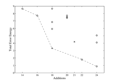
(a) $\epsilon(\bm{\alpha})\,\times\,\mathcal{A}(\bm{\alpha})$

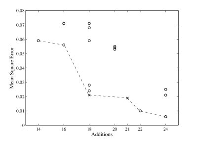
(b) $\operatorname{MSE}(\bm{\alpha})\,\times\,\mathcal{A}(\bm{\alpha})$

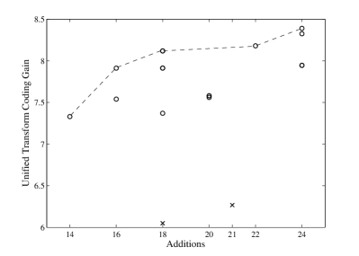
(c) $C_{g}(\bm{\alpha})\,\times\,\mathcal{A}(\bm{\alpha})$

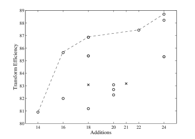
(d) $\eta(\bm{\alpha})\,\times\,\mathcal{A}(\bm{\alpha})$

Figure 2: Assessment plots for the proposed efficient approximations; competing methods were included for comparison.

Fig. 2(a)–(b) indicates that the Feig-Winograd approximations excel in terms of proximity to the original DCT transforms as measured by the total error energy and MSE. Additionally, the Feig-Winograd transforms presented better coding-related figures, except for transformations that require 16 and 18 additions.

In particular, considering transformations that required only 16 additions, we notice that the proposed approximation $\bm{\mathsf{T}}^{(4)}_{8}$ outperformed $\mbox{BAS}^{(6)}$ in terms of total error energy and MSE. However, $\mbox{BAS}^{(6)}$ shows better coding gain performance than $\bm{\mathsf{T}}^{(4)}_{8}$. Now considering transformations demanding 18 additions, we have that approximations $\mbox{BAS}^{(2)}$, $\mbox{BAS}^{(3)}$, $\mbox{BAS}^{(5)}$, and $\mbox{BAS}^{(7)}$ showed better coding gain performance than the proposed transformations $\bm{\mathsf{T}}^{(5)}_{8}$ and $\bm{\mathsf{T}}^{(6)}_{8}$. As expected, the approximation $\bm{\mathsf{T}}^{(1)}_{8}$ has the best coding performance among all considered transforms in Fig. 2. Suggested approximation $\bm{\mathsf{T}}^{(2)}_{8}$ could outperform non-Feig-Winograd transform in all metrics.

In terms of the nonorthogonal transforms $\bm{\mathsf{T}}^{(16)}_{8}$ and $\mbox{BAS}^{(1)}$, we report that $\bm{\mathsf{T}}^{(16)}_{8}$ possesses the smaller total error energy when compared to $\mbox{BAS}^{(1)}$, while presenting a similar performance. However, $\bm{\mathsf{T}}^{(16)}_{8}$ is 14.3% less computationally complex. Also, as discussed in [71], it is generally expected that nonorthogonal transforms present lower values of coding gain compared with orthogonal transforms (cf. Fig. 2(c)). This is expected since coding gain measures are optimized for the KLT [72], which is orthogonal.

We also notice that Figs. 2(a)–2(d) can be interpreted as results of four different bi-objective optimization problems [77, p. 245], where the trade-off between computational cost and performance measures are emphasized. The optimal solutions of the bi-objective optimization problems are situated on the boundary of set of feasible solutions [76, p. 28]. Such boundaries are shown in Fig. 2 and roughly represent the Pareto frontiers for each problem [77, p. 11]. Thus, in this sense, we separate the transforms situated on each Pareto frontier as optimal transformations. Such transforms were: $\bm{\mathsf{T}}^{(1)}_{8}$, $\bm{\mathsf{T}}^{(2)}_{8}$, $\bm{\mathsf{T}}^{(3)}_{8}$, $\bm{\mathsf{T}}^{(4)}_{8}$, $\bm{\mathsf{T}}^{(16)}_{8}$, $\mbox{BAS}^{(1)}$, $\mbox{BAS}^{(2)}$, $\mbox{BAS}^{(6)}$, and $\mbox{BAS}^{(7)}$. This reduced set of transforms was submitted to subsequent image compression analysis.

However, notice that although the remaining transforms $\bm{\mathsf{T}}^{(5)}_{8}$, $\bm{\mathsf{T}}^{(6)}_{8}$, …, $\bm{\mathsf{T}}^{(15)}_{8}$ were outperformed, the performance of a DCT approximation is highly dependent on the envisioned task. Thus, these transforms may be adequate in other contexts, as suggested in [47].

In terms of comparisons with other methods, we notice that current video standards AVC/H.264 [13, 56] and HEVC/H.265 [14, 57, 81] employ integer DCT approximations, which are indeed encompassed in the Feig-Winograd matrix subspace. However, these integer matrices do not satisfy the low-complexity restriction on the matrix elements—namely having its parameter vector defined over the set $\mathcal{P}=\{0,\pm 1/2,\pm 1,\pm 2\}$, as shown in Section 2.5. Possessing large elements, the implementation of such matrices requires more sophisticate operation schemes which make them more computationally expensive [56, 57, 81] when compared to the extremely low-complexity approximations discussed here. For instance, in terms of additive complexity, the AVC requires from 50.00% to 128.57% more operations in comparison with the optimal transformations, as showed in Table 4. On its turn, HEVC requires multiplication operations, which are much more expensive than simple additions [83]. For a fair comparison, we restricted our subsequent analyses to the set of very low-complexity matrices whose elements are in $\mathcal{P}$.

5 Image Compression

In order to evaluate the performance of the selected approximations in image compression, we adopted a JPEG-like computational simulation [8, 84, 41, 44, 45, 46, 42, 47, 48, 40, 49, 68, 21, 24] based on a set of 45 512$\times$512 8-bit greyscale standard images obtained from a public image bank [85]. Images were split into 8$\times$8 sub-blocks, which were submitted to a given 2-D transformation [8, 86] depending on the considered DCT approximation. The 2-D transform operation depends on whether the considered transform is orthogonal or not. Let $\mathbf{A}$ be a 8$\times$8 sub-block of the considered image. In general, the 2-D approximate DCT of $\mathbf{A}$ be written as [86]:

$$\mathbf{B} =\begin{cases}\hat{\mathbf{C}}_{8}\cdot\mathbf{A}\cdot\hat{\mathbf{C}}_{8}^{\top},&\text{if $\mathbf{T}^{(\bm{\alpha})}_{8}$ satisfies~{}\eqref{equation-condition-1},}\\ \hat{\mathbf{C}}_{8}\cdot\mathbf{A}\cdot\hat{\mathbf{C}}_{8}^{-1},&\text{otherwise.}\end{cases}$$

This computation furnished 64 coefficients in the approximate transform domain for each sub-block. According to the standard zigzag sequence [8], only the $r$ initial coefficients in each block were retained and employed to reconstruct the image [48]. All the remaining coefficients were set to zero. We adopted $1\leq r\leq 45$. Based on 8-bit images, this approach implies in the fixed bitrate equals to $r/8$ bpp. After compression, the inverse 2-D transform was applied to reconstruct the processed data. Subsequently, image quality was evaluated.

Above outlined methodology is also described in [6] and supported in [41, 44, 45, 46, 42]. However, in contrast to the JPEG-based image compression experiments described in [6, 41, 44, 45, 46, 42], we adopted average image quality measures from the entire image set [48, 40, 68] instead of the results obtained from particular selected images. Thus, our approach is less prone to variance effects and fortuitous input data, being more robust a methodology [87].

Image degradation was assessed by means of the peak signal-to-noise ratio (PSNR) [88] and the structural similarity index (SSIM) [89]. The PSNR is a quality measure widely used in image processing [88] and the SSIM is regarded as a complementary method for image quality assessment [89]. In fact, the SSIM considers luminance, contrast, and image structure to quantify image degradation, being consistent with subjective quality measurements [90].

Figs. 3(a)–(b) show the obtained quality measures for the transforms identified as optimal according to the discussion at the end of the preceding section. This type of performance curves is commonly employed as a comparison tool in approximate DCT literature [44, 45, 42, 48, 40]. For an improved visualization of the performance curves, we considered the absolute percentage error (APE) relative to the DCT of both the PSNR and SSIM measurements. The resulting values are plotted in Figs. 3(c)–(d). To further validate our methodology, we also computed additional descriptive statistical measures of the results. In particular, the coefficient of variation [91] was found to be consistently less than $16\%$, for all data sample. This fact suggests that adopting average values for the metrics is indeed an adequate approach, as supported in [92, p. 155] and [93, p. 387].

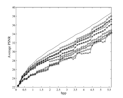
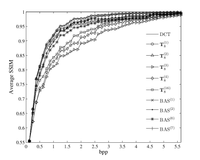
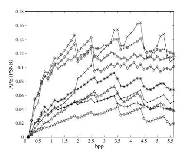
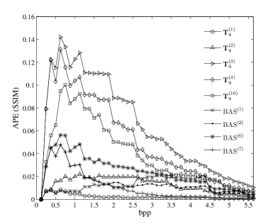
Figure 3: Quality measures of selected optimal approximations for several values of bpp according to the following figures of merit: 3 Average PSNR, 3 Average PSNR absolute percentage error relative to the DCT, 3 Average SSIM, and 3 Average SSIM absolute percentage error relative to the DCT.

As expected, among all considered methods, $\bm{\mathsf{T}}^{(1)}_{8}$ possesses the best performance in terms of image quality at the cost of the highest computational complexity [44, 45, 46]. Feig-Winograd approximation $\bm{\mathsf{T}}^{(2)}_{8}$ could outperform transformations $\bm{\mathsf{T}}^{(3)}_{8}$, $\bm{\mathsf{T}}^{(4)}_{8}$, $\bm{\mathsf{T}}^{(16)}_{8}$, and $\mbox{BAS}^{(6)}$, while exhibiting similar performance to $\mbox{BAS}^{(2)}$ and $\mbox{BAS}^{(7)}$. Transformations $\bm{\mathsf{T}}^{(3)}_{8}$, $\bm{\mathsf{T}}^{(4)}_{8}$, and $\bm{\mathsf{T}}^{(16)}_{8}$ also performed better than $\mbox{BAS}^{(1)}$ in terms of PSNR, for $r>25$ (bitrate larger than 3.125 bpp), and of SSIM, for all values of $r$. The new nonorthogonal $\bm{\mathsf{T}}^{(16)}_{8}$ outperformed $\bm{\mathsf{T}}^{(3)}_{8}$ and $\bm{\mathsf{T}}^{(4)}_{8}$. However, transformation $\bm{\mathsf{T}}^{(16)}_{8}$ showed a lower arithmetic complexity when compared to the also nonorthogonal $\mbox{BAS}^{(1)}$. Proposed approximation $\bm{\mathsf{T}}^{(4)}_{8}$ surpassed $\bm{\mathsf{T}}^{(3)}_{8}$ in both PSNR and SSIM measurements for all compression ratio, requiring only two extra additions for its computation.

Fig. 4 shows 512$\times$512 Lena image after being submitted to the described JPEG-like compression, which provides a qualitative comparison for $r=25$ (3.125 bpp). This corresponds to discarding $60\%$ of the approximate DCT coefficients. PSNR and SSIM measurements are included for comparison.

(a) $\bm{\mathsf{T}}^{(1)}_{8}$ (PSNR=35.176, SSIM=0.995)

(b) $\bm{\mathsf{T}}^{(2)}_{8}$ (PSNR=34.138, SSIM=0.989)

(c) $\bm{\mathsf{T}}^{(3)}_{8}$ (PSNR=31.838, SSIM=0.970)

(d) $\bm{\mathsf{T}}^{(4)}_{8}$ (PSNR=32.299, SSIM=0.977)

(e) $\bm{\mathsf{T}}^{(16)}_{8}$ (PSNR=31.602, SSIM=0.985)

(f) $\mbox{BAS}^{(1)}$ (PSNR=31.452, SSIM=0.980)

(g) $\mbox{BAS}^{(2)}$ (PSNR=34.794, SSIM=0.991)

(h) $\mbox{BAS}^{(6)}$ (PSNR=33.819, SSIM=0.986)

(i) $\mbox{BAS}^{(7)}$ (PSNR=35.433, SSIM=0.995)

(j) DCT (PSNR=37.886, SSIM=0.997)

Figure 4: Compressed Lena image using 4(a) $\bm{\mathsf{T}}^{(1)}_{8}$, 4(b) $\bm{\mathsf{T}}^{(2)}_{8}$, 4(c) $\bm{\mathsf{T}}^{(3)}_{8}$, 4(d) $\bm{\mathsf{T}}^{(4)}_{8}$, 4(e) $\bm{\mathsf{T}}^{(16)}_{8}$, 4(f) $\mbox{BAS}^{(1)}$, 4(g) $\mbox{BAS}^{(2)}$, 4(h) $\mbox{BAS}^{(6)}$, 4(i) $\mbox{BAS}^{(7)}$, and 4(j) DCT, for $r=25$ (3.125 bpp).

6 Conclusion and final remarks

We introduced a new class of matrices based on a parametrization of the Feig-Winograd DCT factorization. By solving a constrained multicriteria optimization problem, several low-complexity DCT approximations were obtained. Among the obtained solutions, we identified DCT approximations already reported in literature. Thus our procedure furnishes a mathematical framework that mathematically unifies them. Moreover, we derived novel DCT approximations. The new transformations were assessed in terms of computational complexity, DCT matrix proximity, coding gain, and performance in JPEG-like compression. The DCT approximations in the Feig-Winograd matrix subspace exhibited roughly a trade-off between cost and performance. The computational complexity of the proposed transforms ranged from 14 to 24 additions and from 0 to 2 bit-shifting operations. It is worth to note that all transforms in the Feig-Winograd class possess the same algorithm structure. Furthermore, the associated inverse transforms share similar mathematical formalism and possess simple fast algorithms. Thus, in terms of circuitry design, one can interchange transforms with minimal hardware modifications. In emerging reconfigurable systems, it may be possible to switch modus operandi based on the demanded picture quality and required energy consumption. Thus, the proposed class of approximations may be a candidate suite of fast algorithms in such context. Besides the image compression context, the Feig-Winograd class of DCT approximations can be applied for data encryption following the scheme introduced in [94, 95]. Finally, we remark that the proposed method is sufficiently flexible to be extended to large blocklengths that are powers of two, according to the Feig-Winograd general theory for DCT factorizaton [31, p. 2188].

References

- [1] K. R. Rao and P. Yip, Discrete Cosine Transform: Algorithms, Advantages, Applications. San Diego, CA: Academic Press, 1990.
- [2] V. Britanak, P. Yip, and K. R. Rao, Discrete Cosine and Sine Transforms. Academic Press, 2007.
- [3] N. Ahmed, T. Natarajan, and K. R. Rao, “Discrete cosine transform,” IEEE Transactions on Computers, vol. C-23, no. 1, pp. 90–93, Jan. 1974.
- [4] R. J. Clarke, “Relation between the Karhunen-Loève and cosine transforms,” IEEE Proceedings F Communications, Radar and Signal Processing, vol. 128, no. 6, pp. 359–360, Nov. 1981.
- [5] J. Liang and T. D. Tran, “Fast multiplierless approximation of the DCT with the lifting scheme,” IEEE Transactions on Signal Processing, vol. 49, pp. 3032–3044, 2001.
- [6] T. I. Haweel, “A new square wave transform based on the DCT,” Signal Processing, vol. 82, pp. 2309–2319, 2001.
- [7] V. Bhaskaran and K. Konstantinides, Image and Video Compression Standards. Boston: Kluwer Academic Publishers, 1997.
- [8] G. Wallace, “The JPEG still picture compression standard,” IEEE Transactions on Consumer Electronics, vol. 38, no. 1, pp. xviii–xxxiv, 1992.
- [9] N. Roma and L. Sousa, “Efficient hybrid DCT-domain algorithm for video spatial downscaling,” EURASIP Journal on Advances in Signal Processing, vol. 2007, no. 2, pp. 1–16, 2007.
- [10] International Organisation for Standardisation, “Generic coding of moving pictures and associated audio information – Part 2: Video,” ISO, ISO/IEC JTC1/SC29/WG11 - Coding of Moving Pictures and Audio, 1994.
- [11] International Telecommunication Union, “ITU-T recommendation H.261 version 1: Video codec for audiovisual services at kbits,” ITU-T, Tech. Rep., 1990.
- [12] ——, “ITU-T recommendation H.263 version 1: Video coding for low bit rate communication,” ITU-T, Tech. Rep., 1995.
- [13] T. Wiegand, G. J. Sullivan, G. Bjontegaard, and A. Luthra, “Overview of the H.264/AVC video coding standard,” IEEE Transactions on Circuits and Systems for Video Technology, vol. 13, no. 7, pp. 560–576, Jul. 2003.
- [14] M. T. Pourazad, C. Doutre, M. Azimi, and P. Nasiopoulos, “HEVC: The new gold standard for video compression: How does HEVC compare with H.264/AVC?” IEEE Consumer Electronics Magazine, vol. 1, no. 3, pp. 36–46, Jul. 2012.
- [15] I. E. Richardson, The H.264 Advanced Video Compression Standard. John Wiley & Sons, 2011.
- [16] J.-B. Lee and H. Kalva, The VC-1 and H.264 Video Compression Standards for Broadband Video Services. Springer, 2008.
- [17] M. Mehrabi, F. Zargari, and M. Ghanbari, “Fast and low complexity method for content accessing and extracting DC-pictures from H.264 coded videos,” IEEE Transactions on Consumer Electronics, vol. 56, no. 3, pp. 1801–1808, 2010.
- [18] Z. He and M. Bystrom, “Improved conversion from DCT blocks to integer cosine transform blocks in H.264/AVC,” IEEE Transactions on Circuits and Systems for Video Technology, vol. 18, no. 6, pp. 851–857, 2008.
- [19] J. M. Moon and J.-H. Kim, “A new low-complexity integer distortion estimation method for H.264/AVC encoder,” IEEE Transactions on Circuits and Systems for Video Technology, vol. 20, no. 2, pp. 207–212, 2010.
- [20] G. J. Sullivan, J.-R. Ohm, W.-J. Han, and T. Wiegand, “Overview of the high efficiency video coding (HEVC) standard,” IEEE Transactions on Circuits and Systems for Video Technology, vol. 22, no. 12, pp. 1649–1668, Dec. 2012.
- [21] A. Edirisuriya, A. Madanayake, R. J. Cintra, and F. M. Bayer, “A multiplication-free digital architecture for 2-D DCT/DST transform for HEVC,” in IEEE 27th Convention of Electrical Electronics Engineers in Israel (IEEEI), 2012, pp. 1–5.
- [22] J.-S. Park, W.-J. Nam, S.-M. Han, and S. Lee, “2-D large inverse transform (1616, 3232) for HEVC (High Efficiency Video Coding),” Journal of Semiconductor Technology and Science, vol. 2, pp. 203–211, 2012.
- [23] S. Y. Park and P. Meher, “Flexible integer DCT architectures for HEVC,” in Circuits and Systems (ISCAS), 2013 IEEE International Symposium on, 2013, pp. 1376–1379.
- [24] U. S. Potluri, A. Madanayake, R. J. Cintra, F. M. Bayer, S. Kulasekera, and A. Edirisuriya, “Improved 8-point approximate DCT for image and video compression requiring only 14 additions,” IEEE Transactions on Circuits and Systems I, vol. 61, no. 6, pp. 1727–1740, 2014.
- [25] M. Vetterli and H. Nussbaumer, “Simple FFT and DCT algorithms with reduced number of operations,” Signal Processing, vol. 6, pp. 267–278, Aug. 1984.
- [26] H. S. Hou, “A fast recursive algorithm for computing the discrete cosine transform,” IEEE Transactions on Acoustic, Signal, and Speech Processing, vol. 6, no. 10, pp. 1455–1461, 1987.
- [27] Z. Wang, “Fast algorithms for the discrete W transform and for the discrete Fourier transform,” IEEE Transactions on Acoustics, Speech and Signal Processing, vol. ASSP-32, pp. 803–816, Aug. 1984.
- [28] B. G. Lee, “A new algorithm for computing the discrete cosine transform,” IEEE Transactions on Acoustics, Speech and Signal Processing, vol. ASSP-32, pp. 1243–1245, Dec. 1984.
- [29] Y. Arai, T. Agui, and M. Nakajima, “A fast DCT-SQ scheme for images,” Transactions of the IEICE, vol. E-71, no. 11, pp. 1095–1097, Nov. 1988.
- [30] C. Loeffler, A. Ligtenberg, and G. Moschytz, “Practical fast 1D DCT algorithms with 11 multiplications,” in Proceedings of the International Conference on Acoustics, Speech, and Signal Processing, 1989, pp. 988–991.
- [31] E. Feig and S. Winograd, “Fast algorithms for the discrete cosine transform,” IEEE Transactions on Signal Processing, vol. 40, no. 9, pp. 2174–2193, 1992.
- [32] B. Vasudev and N. Merhav, “DCT mode conversions for field/frame coded MPEG video,” in IEEE Second Workshop on Multimedia Signal Processing, Dec. 1998, pp. 605–610.
- [33] M. C. Lin, L. R. Dung, and P. K. Weng, “An ultra-low-power image compressor for capsule endoscope,” BioMedical Engineering OnLine, vol. 5, no. 1, pp. 1–8, Feb. 2006. [Online]. Available: http://dx.doi.org/10.1186/1475-925X-5-14
- [34] H. P. L. Arjuna Madanayake, R. J. Cintra, D. Onen, V. S. Dimitrov, and L. Bruton, “Algebraic integer based 88 2-D DCT architecture for digital video processing,” in Proceedings of the IEEE International Symposium on Circuits and Systems (ISCAS), Rio de Janeiro, RJ, 2011, pp. 1247–1250. [Online]. Available: http://ieeexplore.ieee.org/xpl/freeabs˙all.jsp?arnumber=5937796
- [35] N. Rajapaksha, A. Edirisuriya, A. Madanayake, R. J. Cintra, D. Onen, I. Amer, and V. S. Dimitrov, “Asynchronous realization of algebraic integer-based 2D DCT using Achronix Speedster SPD60 FPGA,” Journal of Electrical and Computer Engineering, vol. 2013, pp. 1–9, 2013. [Online]. Available: http://www.hindawi.com/journals/jece/2013/834793/
- [36] A. Edirisuriya, A. Madanayake, V. Dimitrov, R. J. Cintra, and J. Adikari, “VLSI architecture for 8-point AI-based Arai DCT having low area-time complexity and power at improved accuracy,” Journal of Low Power Electronics and Applications, vol. 2, no. 2, pp. 127–142, 2012. [Online]. Available: http://www.mdpi.com/2079-9268/2/2/127/
- [37] A. Madanayake, A. Edirisuriya, R. J. Cintra, V. S. Dimitrov, and N. T. Rajapaksha, “A single-channel architecture for algebraic integer based 88 2-D DCT computation,” IEEE Transactions on Circuits and Systems for Video Technology, vol. PP, no. 99, pp. 2083–2089, 2013.
- [38] M. T. Heideman and C. S. Burrus, Multiplicative complexity, convolution, and the DFT, ser. Signal Processing and Digital Filtering. Springer-Verlag, 1988. [Online]. Available: http://books.google.com.br/books?id=QxWoAAAAIAAJ
- [39] Y.-J. Chen, S. Oraintara, T. Tran, K. Amaratunga, and T. Nguyen, “Multiplierless approximation of transforms with adder constraint,” IEEE Signal Processing Letters, vol. 9, no. 11, pp. 344–347, Nov 2002.
- [40] F. M. Bayer and R. J. Cintra, “DCT-like transform for image compression requires 14 additions only,” Electronics Letters, vol. 48, no. 15, pp. 919–921, 19 2012.
- [41] S. Bouguezel, M. O. Ahmad, and M. N. S. Swamy, “Low-complexity 88 transform for image compression,” Electronics Letters, vol. 44, no. 21, pp. 1249–1250, Sep. 2008.
- [42] ——, “A low-complexity parametric transform for image compression,” in Proceedings of the 2011 IEEE International Symposium on Circuits and Systems, 2011.
- [43] K. Lengwehasatit and A. Ortega, “Scalable variable complexity approximate forward DCT,” IEEE Transactions on Circuits and Systems for Video Technology, vol. 14, no. 11, pp. 1236–1248, Nov. 2004.
- [44] S. Bouguezel, M. O. Ahmad, and M. N. S. Swamy, “A multiplication-free transform for image compression,” in 2nd International Conference on Signals, Circuits and Systems (SCS), Nov. 2008, pp. 1–4.
- [45] ——, “A fast 88 transform for image compression,” in 2009 International Conference on Microelectronics (ICM), Dec. 2009, pp. 74–77.
- [46] ——, “A novel transform for image compression,” in 53rd IEEE International Midwest Symposium on Circuits and Systems (MWSCAS), Aug. 2010, pp. 509–512.
- [47] ——, “Binary discrete cosine and Hartley transforms,” IEEE Transactions on Circuits and Systems I: Regular Papers, vol. 60, no. 4, pp. 989–1002, 2013.
- [48] R. J. Cintra and F. M. Bayer, “A DCT approximation for image compression,” IEEE Signal Processing Letters, vol. 18, no. 10, pp. 579–582, Oct. 2011.
- [49] U. S. Potluri, A. Madanayake, R. J. Cintra, F. M. Bayer, and N. Rajapaksha, “Multiplier-free DCT approximations for RF multi-beam digital aperture-array space imaging and directional sensing,” Measurement Science and Technology, vol. 23, no. 11, p. 114003, 2012. [Online]. Available: http://stacks.iop.org/0957-0233/23/i=11/a=114003
- [50] W.-K. Kuo and K.-W. Wu, “Traffic prediction and QoS transmission of real-time live VBR videos in WLANs,” ACM Transactions on Multimedia Computing, Communications and Applications, vol. 7, no. 4, pp. 36:1–36:21, Dec. 2011. [Online]. Available: http://doi.acm.org/10.1145/2043612.2043614
- [51] S. Saponara, “Real-time and low-power processing of 3D direct/inverse discrete cosine transform for low-complexity video codec,” Journal of Real-Time Image Processing, vol. 7, pp. 43–53, 2012. [Online]. Available: http://dx.doi.org/10.1007/s11554-010-0174-5
- [52] V. Lecuire, L. Makkaoui, and J.-M. Moureaux, “Fast zonal DCT for energy conservation in wireless image sensor networks,” Electronics Letters, vol. 48, no. 2, pp. 125–127, 2012.
- [53] MATLAB, version 8.1 (R2013a) Documentation. Natick, Massachusetts: The MathWorks Inc., 2013.
- [54] A. K. Jain, Fundamentals of digital image processing. Upper Saddle River, N. J., USA: Prentice-Hall, Inc., 1989. [Online]. Available: http://www.amazon.com/Fundamentals-Digital-Image-Processing-Anil/dp/0133361659
- [55] I. N. Herstein, Topics in algebra, 2nd ed. Wiley India Pvt. Limited, 2006. [Online]. Available: http://books.google.com.br/books?id=6N2aoMYbYQMC
- [56] S. Gordon, D. Marpe, and T. Wiegand, “Simplified use of 88 transform – updated proposal and results,” Joint Video Team (JVT) of ISO/IEC MPEG and ITU-T VCEG, doc. JVT–K028, Munich, Germany, Mar 2004.
- [57] A. Fuldseth, G. Bjøntegaard, M. Budagavi, and V. Sze, “CE10: Core transform design for HEVC,” Joint Collaborative Team on Video Coding (JCT-VC), November 2011.
- [58] B. N. Flury and W. Gautschi, “An algorithm for simultaneous orthogonal transformation of several positive definite symmetric matrices to nearly diagonal form,” SIAM Journal on Scientific and Statistical Computing, vol. 7, no. 1, pp. 169–184, Jan. 1986. [Online]. Available: http://dx.doi.org/10.1137/0907013
- [59] W. L. Briggs and V. E. Henson, The DFT: An Owners’ Manual for the Discrete Fourier Transform, ser. Miscellaneous Bks. Society for Industrial and Applied Mathematics, 1995. [Online]. Available: http://books.google.com.br/books?id=coq49“˙LRURUC
- [60] K. Cheung and K. Tong, “Proposed data compression schemes for the Galileo S-Band contingency mission,” in Space and Earth Science Data Compression Workshop Proceedings, Snowbird, Utah, 1993, pp. 99–109.
- [61] D. S. Watkins, Fundamentals of Matrix Computations, ser. Pure and Applied Mathematics: A Wiley Series of Texts, Monographs and Tracts. Wiley, 2004. [Online]. Available: http://books.google.es/books?id=xi5omWiQ-3kC
- [62] N. J. Higham, Functions of Matrices: Theory and Computation, ser. SIAM e-books. Society for Industrial and Applied Mathematics (SIAM, 3600 Market Street, Floor 6, Philadelphia, PA 19104), 2008. [Online]. Available: http://books.google.com.br/books?id=S6gpNn1JmbgC
- [63] ——, “Computing the polar decomposition—with applications,” SIAM Journal on Scientific and Statistical Computing, vol. 7, no. 4, pp. 1160–1174, Oct. 1986.
- [64] N. J. Higham and R. S. Schreiber, “Fast polar decomposition of an arbitrary matrix,” Ithaca, NY, USA, Tech. Rep., 1988.
- [65] R. J. Cintra, “An integer approximation method for discrete sinusoidal transforms,” Journal of Circuits, Systems, and Signal Processing, vol. 30, no. 6, pp. 1481–1501, 2011. [Online]. Available: http://www.springerlink.com/content/nw5u0267254t3683/
- [66] N. J. Higham, “Computing real square roots of a real matrix,” Linear Algebra and its Applications, vol. 88–89, pp. 405–430, 1987. [Online]. Available: http://www.sciencedirect.com/science/article/pii/0024379587901182
- [67] N. J. Higham, D. S. Mackey, N. Mackey, and F. Tisseur, “Computing the polar decomposition and the matrix sign decomposition in matrix groups.” SIAM J. Matrix Analysis Applications, vol. 25, no. 4, pp. 1178–1192, 2004. [Online]. Available: http://dblp.uni-trier.de/db/journals/siammax/siammax25.html#HighamMMT04
- [68] F. M. Bayer, R. J. Cintra, A. Edirisuriya, and A. Madanayake, “A digital hardware fast algorithm and FPGA-based prototype for a novel 16-point approximate DCT for image compression applications,” Measurement Science and Technology, vol. 23, no. 8, p. 114010, 2012.
- [69] G. A. F. Seber, A Matrix Handbook for Statisticians. John Wiley & Sons, Inc, 2008.
- [70] Z. Wang and A. C. Bovik, “Mean squared error: Love it or leave it? A new look at signal fidelity measures,” IEEE Signal Processing Magazine, vol. 26, no. 1, pp. 98–117, Jan. 2009.
- [71] J. Katto and Y. Yasuda, “Performance evaluation of subband coding and optimization of its filter coefficients,” Journal of Visual Communication and Image Representation, vol. 2, no. 4, pp. 303–313, 1991. [Online]. Available: http://www.sciencedirect.com/science/article/pii/1047320391900114
- [72] V. K. Goyal, “Theoretical foundations of transform coding,” IEEE Signal Processing Magazine, vol. 18, no. 5, pp. 9–21, 2001.
- [73] G. Strang, “The discrete cosine transform,” SIAM Rev., vol. 41, no. 1, pp. 135–147, Mar. 1999. [Online]. Available: http://dx.doi.org/10.1137/S0036144598336745
- [74] J. K. Merikoski, “On the trace and the sum of elements of a matrix,” Linear Algebra and its Applications, vol. 60, pp. 177–185, 1984. [Online]. Available: http://www.sciencedirect.com/science/article/pii/0024379584900788
- [75] W. K. Cham, “Development of integer cosine transforms by the principle of dyadic symmetry,” in IEE Proceedings I Communications, Speech and Vision, vol. 136, no. 4, 1989, pp. 276–282.
- [76] M. Ehrgott, Multicriteria Optimization, ser. Lecture Notes in Economics and Mathematical Systems. Springer-Verlag GmbH, 2000. [Online]. Available: http://books.google.com.br/books?id=au6PMgEACAAJ
- [77] K. Miettinen, Nonlinear Multiobjective Optimization, ser. International series in operations research and management science. Kluwer Academic Publishers, 1999. [Online]. Available: http://books.google.com.br/books?id=ha“˙zLdNtXSMC
- [78] L. S. Oliveira and S. F. P. Saramago, “Multiobjective optimization techniques applied to engineering problems,” Journal of the Brazilian Society of Mechanical Sciences and Engineering, vol. 32, pp. 94 – 105, 03 2010. [Online]. Available: http://www.scielo.br/scielo.php?script=sci˙arttext&pid=S1678-58782010000100012&nrm=iso
- [79] T. W. Hungerford, Algebra, ser. Graduate Texts in Mathematics. Springer, 1974. [Online]. Available: http://books.google.com.br/books?id=t6N“˙tOQhafoC
- [80] G. Strang and T. Nguyen, Wavelets and Filter Banks. Wellesley-Cambridge Press, 1996.
- [81] P. K. Meher, S. Y. Park, B. K. Mohanty, K. S. Lim, and C. Yeo, “Efficient integer DCT architectures for HEVC,” IEEE Transactions on Circuits and Systems For Video Technology, vol. 24, no. 1, pp. 168–178, January 2014.
- [82] K. J. Horadam, Hadamard Matrices and Their Applications. Princeton University Press, 2007. [Online]. Available: http://books.google.com.br/books?id=fZ3quix-ifMC
- [83] R. E. Blahut, Fast Algorithms for Signal Processing. Cambridge University Press, 2010.
- [84] W. B. Pennebaker and J. L. Mitchell, JPEG Still Image Data Compression Standard. New York, NY: Van Nostrand Reinhold, 1992.
- [85] “The USC-SIPI image database,” http://sipi.usc.edu/database/, 2011, University of Southern California, Signal and Image Processing Institute.
- [86] T. Suzuki and M. Ikehara, “Integer DCT based on direct-lifting of DCT-IDCT for lossless-to-lossy image coding,” IEEE Transactions on Image Processing, vol. 19, no. 11, pp. 2958–2965, Nov. 2010.
- [87] S. M. Kay, Fundamentals of Statistical Signal Processing, Volume I: Estimation Theory, ser. Prentie Hall Signal Processing Series, A. V. Oppenheim, Ed. Upper Saddle River, NJ: Prentice Hall, 1993, vol. 1.
- [88] Q. Huynh-Thu and M. Ghanbari, “Scope of validity of PSNR in image/video quality assessment,” Electronics Letters, vol. 44, no. 13, pp. 800–801, Jun. 2008.
- [89] Z. Wang, A. C. Bovik, H. R. Sheikh, and E. P. Simoncelli, “Image quality assessment: from error visibility to structural similarity,” IEEE Transactions on Image Processing, vol. 13, no. 4, pp. 600–612, Apr. 2004.
- [90] Z. Wang and A. C. Bovik, “Reduced- and no-reference image quality assessment,” IEEE Signal Processing Magazine, vol. 28, no. 6, pp. 29–40, 2011.
- [91] H. Abdi, “Coefficient of variation,” Encyclopedia of Research Design. SAGE Publications, Inc., Thousand Oaks, CA, pp. 169–171, 2010.
- [92] C. Brown, Applied Multivariate Statistics in Geohydrology and Related Sciences. Springer, 1998. [Online]. Available: http://books.google.com.br/books?id=Y8gPAQAAIAAJ
- [93] D. Wackerly, W. Mendenhall, and R. Scheaffer, Mathematical Statistics with Applications. Cengage Learning, 2007. [Online]. Available: http://books.google.es/books?id=ZvPKTemPsY4C
- [94] L. Chen and D. Zhao, “Optical image encryption with Hartley transforms,” Optics Letters, vol. 31, no. 23, pp. 3438–3440, Dec 2006.
- [95] S. Bouguezel, M. O. Ahmad, and M. N. S. Swamy, “Image encryption using the reciprocal-orthogonal parametric transform,” in Proceedings of 2010 IEEE International Symposium on Circuits and Systems (ISCAS), 2010, pp. 2542–2545.