Near-infrared light curves of Type Ia supernovae: Studying properties of the second maximum

Abstract

Type Ia supernovae have been proposed to be much better distance indicators at near-infrared compared to optical wavelengths – the effect of dust extinction is expected to be lower and it has been shown that SNe Ia behave more like ‘standard candles’ at NIR wavelengths. To better understand the physical processes behind this increased uniformity, we have studied the $Y$, $J$ and $H$-filter light curves of 91 SNe Ia from the literature. We show that the phases and luminosities of the first maximum in the NIR light curves are extremely uniform for our sample. The phase of the second maximum, the late-phase NIR luminosity and the optical light curve shape are found to be strongly correlated, in particular more luminous SNe Ia reach the second maximum in the NIR filters at a later phase compared to fainter objects. We also find a strong correlation between the phase of the second maximum and the epoch at which the SN enters the Lira law phase in its optical colour curve (epochs $\sim$ 15 to 30 days after $B$ band maximum). The decline rate after the second maximum is very uniform in all NIR filters. We suggest that these observational parameters are linked to the nickel and iron mass in the explosion, providing evidence that the amount of nickel synthesised in the explosion is the dominating factor shaping the optical and NIR appearance of SNe Ia.

1 Introduction

The uniformity of Type Ia supernovae (SNe Ia) has led to their use, after calibration, as distance indicators [reviewed in:][]Goobar2011 and they provided the first evidence for the accelerated expansion of the Universe Riess1998,Perlmutter1999.

Observations of large SN Ia samples show that the peak luminosity in the optical is not uniform but can be normalised following a variety of calibration techniques, most notably the correlation between light curve shape and peak luminosity, and between light curve colour and peak luminosity [e.g.][]Phillips1993, Riess1996, Guy2005, Guy2007, Guy2010, Jha2007. The variation in bolometric luminosity for the objects Contardo2000 implies variations in the physical parameters of the explosion, in particular the synthesised Ni mass and the total ejected mass Stritzinger2006, Scalzo2014.

At near-infrared (NIR) wavelengths (900nm $>\lambda>$ 2000nm), SNe Ia have a very uniform brightness distribution without any prior normalisation Elias1981, Meikle2000, K04a, K07. The scatter in the peak luminosity in these studies is $\sim$0.2 mag, which when combined with the lower sensitivity of the NIR to extinction by dust, has sparked interest in the use of this wavelength region. Following large observational campaigns, statistically significant samples of SN Ia light curves have been made public WV08, Contreras2010, Stritzinger2011, BN12, and have been used to construct the first rest-frame NIR Hubble diagrams Nobili2005,Freedman2009, Kattner2012, Weyant2014.

Dust extinction in the NIR is significantly reduced compared to the optical leading to smaller corrections and uncertainties. In addition to the photometric calibration systematics [see][]Conley2011 the dust extinction for SNe Ia is one of the major sources of systematics in SN Ia cosmology measurements [e.g.][]Peacock2006, Goobar2011. In particular, extinction law measurements for galaxies remains uncertain [see discussions in][]Phillips2013, Scolnic2014. The recent SN 2014J is a case in point with derived dust properties very different from local interstellar dust Amanullah2014, Foley2014. Strongly reddened SNe Ia may also exhibit variations in their light curve shapes Leibundgut1988, Amanullah2014.

The light-curve morphology in the NIR is markedly different from that in the optical with a pronounced second maximum in $IYJHK$ filters for ‘normal’ SNe Ia Elias1981, Elias1985, Leibundgut1988, Leibundgut2000, Meikle2000, WV08, Folatelli2010. The formation of the NIR spectrum in SNe Ia is highly sensitive to the opacity variations Spyr1994, Wheeler1998 as the spectrum is dominated by line blanketing opacity making the evolution of the NIR light a sensitive probe of the structure of the ejecta. [Kasen2006] in a detailed study suggested that the second maximum is a result of a decrease in opacity due to the ionisation change of Fe group elements from doubly to singly ionised atoms, which preferentially radiate the energy at near-IR wavelengths. A direct prediction of Kasen2006 is that a larger iron mass leads to a later NIR second maximum.

Studies of the $i$ band light curve find a relation between the phase of the second maximum and the optical light curve shape [e.g. $\Delta m_{15}(B)$, ][]Folatelli2010, Hamuy1996. The strength of the second maximum in $i$ does not show such a correlation.

In this paper, we investigate the properties of SN Ia NIR light curves ($YJH$) and establish correlations with other observational characteristics. Connections to possible physical properties in the explosions are explored. The structure of this paper is as follows: after a presentation of the input data in Section 2, we analyse the NIR light curve properties (Section 3) along with a description of NIR colours. Correlations with optical light curve parameters and their interpretations are given in §4 followed by a discussion in §5. The conclusions are presented in Section 6.

2 Data

Table 1: SN sample

SN name	Phase range			$N_{i}$	$N_{Y}$	$N_{J}$	$N_{H}$	$N_{K}$	Reference
	(days)
SN1980N	$5.7$	$\cdots$	$99.7$	…	…	11	13	…	M00
SN1981B	$2.7$	$\cdots$	$120.5$	…	…	17	17	…	M00
SN1986G	$-6.1$	$\cdots$	$101.0$	…	…	28	29	…	M00
SN1998bu	$-8.5$	$\cdots$	$31.5$	…	…	23	23	…	M00
SN1999ac	$-13.1$	$\cdots$	$63.8$	…	…	30	30	…	Ph06
SN1999ee	$-7.5$	$\cdots$	$27.5$	…	17	18	20	…	K04a
SN1999ek	$-8.0$	$\cdots$	$23.0$	…	…	14	15	…	K04a
SN2000E	$-7.7$	$\cdots$	$126.6$	…	…	18	18	…	V03
SN2000bh	$-5.5$	$\cdots$	$39.0$	…	6	21	22	…	K04a
SN2001ba	$-6.0$	$\cdots$	$34.9$	…	…	14	15	…	K04a
SN2001bt	$-1.6$	$\cdots$	$65.3$	…	…	21	21	…	K04a
SN2001cn	$4.2$	$\cdots$	$59.1$	…	…	19	19	…	K04b
SN2001cz	$-2.4$	$\cdots$	$47.6$	…	…	12	12	…	K04b
SN2001el	$-10.6$	$\cdots$	$64.3$	…	…	33	32	…	K03
SN2002bo	$-11.0$	$\cdots$	$44.0$	…	…	17	17	17	K04b, ESC
SN2002dj	$-11.0$	$\cdots$	$67.0$	…	…	21	21	…	P08, ESC
SN2002fk	$-12.2$	$\cdots$	$102.1$	…	…	24	23	23	C13
SN2003cg	$-6.4$	$\cdots$	$413.5$	…	…	13	13	…	ER06, ESC
SN2003hv	$1.2$	$\cdots$	$62.0$	…	16	16	16	…	L09, ESC
SN2004ef	$-8.7$	$\cdots$	$65.2$	46	4	3	4	3	CSP
SN2004eo	$-12.0$	$\cdots$	$63.0$	39	8	9	9	8	CSP, P07, ESC
SN2004ey	$-8.9$	$\cdots$	$48.1$	32	7	9	9	8	CSP
SN2004gs	$-3.6$	$\cdots$	$99.1$	50	12	11	10	…	CSP
SN2004gu	$-0.4$	$\cdots$	$48.6$	27	8	7	7	…	CSP
SN2005A	$-3.5$	$\cdots$	$30.4$	35	10	10	10	…	CSP
SN2005M	$-8.0$	$\cdots$	$74.7$	56	17	17	14	12	CSP
SN2005ag	$-1.7$	$\cdots$	$66.3$	44	9	9	9	…	CSP
SN2005al	$-1.0$	$\cdots$	$82.0$	35	7	8	8	7	CSP
SN2005am	$-4.6$	$\cdots$	$75.3$	36	6	6	6	6	CSP
SN2005el	$-7.3$	$\cdots$	$83.6$	25	21	22	15	3	CSP
SN2005eq	$-3.6$	$\cdots$	$97.3$	27	15	15	10	1	CSP
SN2005hc	$-4.5$	$\cdots$	$84.4$	22	13	11	9	…	CSP
SN2005hj	$-2.3$	$\cdots$	$87.6$	16	11	12	10	1	CSP
SN2005iq	$-5.3$	$\cdots$	$67.7$	19	11	11	11	1	CSP
SN2005kc	$-10.4$	$\cdots$	$30.6$	13	9	9	8	…	CSP
SN2005ki	$-9.9$	$\cdots$	$155.8$	47	12	11	10	…	CSP
SN2005na	$-1.8$	$\cdots$	$94.0$	27	14	11	12	…	CSP
SN2006D	$-6.0$	$\cdots$	$112.8$	42	17	16	16	6	CSP
SN2006X	$-11.0$	$\cdots$	$119.8$	39	32	33	32	9	CSP, ESC
SN2006ax	$-11.7$	$\cdots$	$71.2$	26	19	18	16	3	CSP
SN2006bh	$-4.9$	$\cdots$	$60.0$	24	12	11	10	…	CSP
SN2006br	$5.8$	$\cdots$	$37.7$	9	5	5	5	…	CSP
SN2006ej	$4.4$	$\cdots$	$69.4$	13	3	3	3	…	CSP
SN2006eq	$0.2$	$\cdots$	$43.0$	18	10	7	8	…	CSP
SN2006et	$-7.2$	$\cdots$	$105.7$	23	18	12	13	…	CSP
SN2006ev	$4.2$	$\cdots$	$48.1$	12	10	8	8	…	CSP
SN2006gj	$-1.8$	$\cdots$	$96.0$	19	13	10	4	…	CSP
SN2006gt	$-2.1$	$\cdots$	$62.8$	13	10	8	6	…	CSP
SN2006hb	$7.2$	$\cdots$	$136.9$	25	10	10	9	…	CSP
SN2006hx	$-9.3$	$\cdots$	$30.7$	8	7	6	5	…	CSP
SN2006is	$6.4$	$\cdots$	$118.2$	24	8	8	7	…	CSP
SN2006kf	$-4.8$	$\cdots$	$86.0$	20	17	14	11	3	CSP
SN2006lu	$5.1$	$\cdots$	$90.1$	21	6	4	3	…	CSP
SN2006ob	$-2.6$	$\cdots$	$58.3$	13	12	9	5	…	CSP
SN2006os	$2.4$	$\cdots$	$57.3$	14	10	6	5	…	CSP
SN2007A	$-4.7$	$\cdots$	$18.3$	9	9	5	3	…	CSP
SN2007S	$-10.5$	$\cdots$	$102.2$	19	12	17	18	7	CSP
SN2007af	$-8.8$	$\cdots$	$82.1$	28	26	25	24	5	CSP
SN2007ai	$-0.4$	$\cdots$	$86.4$	17	7	7	6	3	CSP
SN2007as	$-0.0$	$\cdots$	$77.7$	19	11	10	10	…	CSP
SN2007bc	$-3.0$	$\cdots$	$58.8$	10	11	8	6	…	CSP
SN2007bd	$-9.5$	$\cdots$	$215.8$	14	12	9	7	…	CSP
SN2007bm	$-0.2$	$\cdots$	$34.7$	10	10	9	7	…	CSP
SN2007ca	$-8.8$	$\cdots$	$32.1$	12	10	8	7	2	CSP
SN2007if	$14.4$	$\cdots$	$100.2$	16	8	7	5	…	CSP
SN2007jg	$-3.1$	$\cdots$	$58.8$	18	8	6	5	…	CSP
SN2007le	$-11.5$	$\cdots$	$71.2$	26	17	17	16	…	CSP
SN2007nq	$-1.4$	$\cdots$	$77.5$	25	19	10	4	…	CSP
SN2007on	$-8.6$	$\cdots$	$88.2$	38	29	28	25	7	CSP
SN2008C	$2.9$	$\cdots$	$85.6$	19	15	13	18	1	CSP
SN2008R	$-1.3$	$\cdots$	$32.6$	12	8	7	5	…	CSP
SN2008bc	$-9.3$	$\cdots$	$96.6$	32	7	12	11	…	CSP
SN2008bq	$-0.8$	$\cdots$	$43.1$	16	4	4	4	…	CSP
SN2008fp	$-6.0$	$\cdots$	$89.9$	28	22	20	20	7	CSP
SN2008gp	$-10.5$	$\cdots$	$34.4$	19	10	11	9	…	CSP
SN2008hv	$-10.5$	$\cdots$	$78.3$	25	18	16	16	…	CSP
SN2008ia	$-3.5$	$\cdots$	$43.5$	15	16	15	14	…	CSP
PTF09dlc	$-5.56$	$\cdots$	$19.5$	…	…	4	4	…	BN12
PTF10hdv	$-3.9$	$\cdots$	$10.3$	…	…	4	4	…	BN12
PTF10hmv	$-10.1$	$\cdots$	$7.9$	…	…	…	5	…	BN12
PTF10mwb	$-12.3$	$\cdots$	$5.7$	…	…	5	5	…	BN12
PTF10ndc	$-3.9$	$\cdots$	$5.1$	…	…	4	4	…	BN12
PTF10nlg	$-5.1$	$\cdots$	$3.9$	…	…	3	5	…	BN12
PTF10qyx	$-3.5$	$\cdots$	$7.5$	…	…	4	4	…	BN12
PTF10tce	$-6.6$	$\cdots$	$6.5$	…	…	4	4	…	BN12
PTF10ufj	$-9.0$	$\cdots$	$4.1$	…	…	4	4	…	BN12
PTF10wnm	$-7.1$	$\cdots$	$4.8$	…	…	4	4	…	BN12
PTF10wof	$-3.9$	$\cdots$	$9.1$	…	…	4	4	…	BN12
PTF10xyt	$-4.6$	$\cdots$	$7.3$	…	…	2	5	…	BN12
SN2011fe	$-16.0$	$\cdots$	$45.9$	…	…	32	35	32	M12
SN2014J	$-10.0$	$\cdots$	$72.4$	…	…	24	24	24	F14

We investigate a large sample of nearby objects with well-sampled optical and NIR data (Table 1). The main data source of NIR SN Ia photometry is the Carnegie SN Project [CSP;][]Contreras2010, Burns2011, Stritzinger2011, Phillips2012, Burns2014. The low-redshift CSP provides a sample of SNe Ia with optical and NIR light curves in a homogeneous and well-defined photometric system (in Vega magnitude system) and thus forms an ideal basis for the evaluation of light curve properties. CSP relies primarily on SN discoveries from the Lick Observatory SN Search [LOSS;][]Leaman2011. The CSP has published light curves on a total of 82 SNe Ia of which 70 have photometry in $YJHK$ bands.

From the CSP NIR dataset, we removed spectroscopically peculiar objects such as SN2006bt and SN2006ot. We also rejected SNe Ia with spectra similar to the peculiar SN 1991bg Filippenko1992, Leibundgut1993, Mazzali1997 and objects that do not exhibit a second maximum (SNe 2005bl, 2005ke, 2005ku, 2006bd, 2006mr, 2007N, 2007ax, 2007ba, 2009F).

We have included in our sample near-IR SN Ia photometry from [Meikle2000] and several SNe Ia observed by the European SN Consortium [ESC;][]Benetti2004, Pignata2008, ER06, Pastorello2007, Krisciunas2009. Twelve SNe Ia have been discussed by BN12 and have data only near the first maximum. We also included NIR photometry from two recent nearby explosions, SN2011fe Matheson2012 and SN2014J Foley2014.

The 91 objects used in this work are listed in Table 1, where the phase range of observations (first and last observation), total number of observations in each filter and the reference for each data set are tabulated. The sample is dominated by SNe Ia from the CSP and we show the results separately for the CSP and non-CSP objects. It is worth noting that there are 15 SNe Ia with observed NIR light curves beyond 100 days.

As can be seen in Table 1 and displayed in Fig. 1, the $K$-band light curves are sparsely sampled and not enough objects are available for detailed analysis. Therefore, we exclude the K-band light curves from further analysis.

3 NIR Light Curve Morphology

In parameterising the NIR light curves we follow the nomenclature introduced by Biscardi2012. The first maximum in filter $X$, $M_{1}(X)$ is reached at a phase, $t_{1}(X)$ relative to the phase of the $B$ maximum ($t^{max}_{B}$=0 d). The light curves dip to a minimum $M_{0}(X)$ at $t_{0}(X)$ before reaching a second maximum, $M_{2}(X)$ at time, $t_{2}(X)$. These three prominent features are shown in Fig. 1. The light curves are plotted without normalisation for phase or corrections for possible differences in photometric systems or absorption.

3.1 Light curve fitting

We fit the optical light curves using the programme SNooPy Burns2011 to determine the peak of the $B$-band light curve through cubic-spline fitting and determine the phase, $t^{max}_{B}$ used throughout this work and the peak brightness $m^{max}_{B}$. SNooPY also determines the $\Delta m_{15}$ parameter commonly used to characterise the SN light curve shape and provides an estimate of the extinction in the host galaxy. The SNooPy light curve fit parameters and distance moduli for the SNe Ia in our sample are given in Table 2. We used the published values of the distance modulus, $\mu$, for non-CSP objects, (references in Table 2). The distance moduli for CSP SNe Ia not in the Hubble flow are taken from Contreras2010 and Stritzinger2011, and the individual references are listed in Table  2. The distance moduli for the rest of the SNe are based on the host galaxy redshift from the NASA/IPAC Extragalactic Database adopting a Hubble constant of $H_{0}$=70 km s^-1 Mpc^-1.

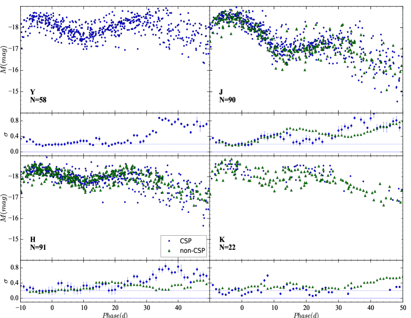
Figure 1: The $Y$, $J$, $H$ and $K$ absolute magnitude light curves of SNe Ia. The CSP sample is shown as blue pentagons. The green triangles indicate the non-CSP sample (see Table 1 for the references). The root-mean-square (RMS) scatter for each day is shown in the lower panels. For guidance a line at a scatter of 0.2 magnitudes is drawn in each panel. The luminosities are based on the literature distances (cf. Table 2) and no correction has been applied. The steady increase of the scatter after the first maximum is evident.

Table 2: Timing of $B_{max}$, $\Delta m_{15}$, distance modulus for the SN in our sample. References for the published distance moduli are provided in the footnote.

SN Name	$t(B_{max})$	err	$\Delta m_{15}$	err	$\mu$	err
	(MJD)		(mag)		(mag)
SN1980N	44585.8	0.5	1.28	0.04	31.59	0.10
SN1981B	44672.0	0.2	1.10	0.04	30.95	0.07
SN1986G	46561.0	0.1	1.76	0.10	28.01	0.12
SN1998bu	50953.3	0.5	1.01	0.02	30.20	0.10
SN1999ac	51251.0	0.5	1.34	0.02	33.50	0.30
SN1999ee	51469.1	0.5	1.09	0.02	33.20	0.20
SN1999ek	51481.8	0.1	1.17	0.03	34.40	0.30
SN2000E	51557.0	0.5	0.99	0.02	31.90	0.40
SN2000bh	51635.2	0.5	1.16	0.01	34.60	0.30
SN2001ba	52034.5	0.5	0.97	0.05	35.40	0.50
SN2001bt	52063.4	0.5	1.18	0.02	34.10	0.40
SN2001cn	52071.6	0.2	1.15	0.02	34.10	0.30
SN2001cz	52103.9	0.1	1.05	0.07	33.50	0.10
SN2001el	52182.5	0.5	1.13	0.04	31.30	0.20
SN2002bo	52356.5	0.2	1.12	0.02	31.80	0.20
SN2002dj	52450.0	0.7	1.08	0.02	32.90	0.30
SN2002fk	52547.9	0.3	1.02	0.04	32.59	0.15
SN2003cg	52729.4	0.5	1.12	0.04	31.28	0.20
SN2003hv	52891.2	0.3	1.09	0.02	31.40	0.30
SN2004ef	53264.4	0.1	1.45	0.01	35.57	0.07
SN2004eo	53278.4	0.1	1.32	0.01	34.03	0.10
SN2004ey	53304.3	0.1	1.02	0.01	34.01	0.12
SN2004gs	53356.2	0.1	1.53	0.01	35.40	0.08
SN2004gu	53362.2	0.2	0.80	0.01	36.59	0.04
SN2005A	53379.7	0.2	1.08	0.02	34.51	0.11
SN2005M	53405.4	0.1	0.80	0.04	35.01	0.09
SN2005ag	53413.7	0.2	0.87	0.01	37.80	0.03
SN2005al	53430.5	0.1	1.30	0.01	33.79	0.15
SN2005am	53436.9	0.1	1.48	0.01	32.85	0.20
SN2005el	53647.0	0.1	1.40	0.01	34.04	0.14
SN2005eq	53654.4	0.1	0.82	0.01	35.46	0.07
SN2005hc	53666.7	0.1	0.80	0.01	36.50	0.05
SN2005hj	53673.8	0.2	0.80	0.02	37.03	0.04
SN2005iq	53687.7	0.1	1.28	0.01	35.80	0.15
SN2005kc	53697.7	0.1	1.12	0.02	33.89	0.15
SN2005ki	53705.5	0.1	1.36	0.01	34.73	0.10
SN2005na	53740.2	0.1	1.03	0.01	35.34	0.08
SN2006D	53757.7	0.1	1.47	0.01	33.00	0.15
SN2006X	53786.3	0.1	1.09	0.03	30.91	0.08
SN2006ax	53827.2	0.1	1.04	0.01	34.46	0.11
SN2006bh	53833.6	0.1	1.42	0.01	33.28	0.20
SN2006br	53853.7	0.6	1.45	0.05	35.23	0.08
SN2006ej	53976.4	0.2	1.37	0.01	34.62	0.11
SN2006eq	53975.9	0.4	1.88	0.04	36.66	0.04
SN2006et	53993.7	0.1	0.88	0.01	34.82	0.10
SN2006ev	53990.1	0.3	1.34	0.01	35.40	0.08
SN2006gj	54000.3	0.2	1.56	0.04	35.42	0.08
SN2006gt	54003.1	0.3	1.71	0.03	36.43	0.05
SN2006hb	54006.0	0.3	1.69	0.02	34.11	0.13
SN2006hx	54021.9	0.2	1.07	0.05	36.47	0.05
SN2006is	54007.5	0.4	0.80	0.01	35.69	0.07
SN2006kf	54041.3	0.1	1.51	0.01	34.78	0.10
SN2006lu	54034.4	0.2	0.92	0.01	36.92	0.04
SN2006ob	54063.4	0.1	1.51	0.01	37.08	0.04
SN2006os	54063.9	0.2	1.08	0.02	35.70	0.07
SN2007A	54113.1	0.2	1.06	0.04	34.26	0.13
SN2007S	54143.8	0.1	0.81	0.01	34.06	0.14
SN2007af	54174.4	0.1	1.11	0.01	32.10	0.10
SN2007ai	54173.5	0.3	0.84	0.02	35.73	0.07
SN2007as	54181.3	0.4	1.27	0.03	34.45	0.12
SN2007bc	54200.3	0.2	1.27	0.02	34.89	0.10
SN2007bd	54206.9	0.1	1.27	0.01	35.73	0.07
SN2007bm	54224.1	0.2	1.11	0.02	32.30	0.07
SN2007ca	54227.7	0.2	1.05	0.03	34.04	0.14
SN2007if	54343.1	0.6	1.07	0.03	37.59	0.03
SN2007jg	54366.1	0.3	1.09	0.04	36.03	0.06
SN2007le	54399.3	0.1	1.03	0.02	32.34	0.08
SN2007nq	54398.8	0.1	1.49	0.01	36.44	0.05
SN2007on	54419.8	0.4	1.65	0.04	31.45	0.08
SN2008C	54466.1	0.2	1.08	0.02	34.34	0.12
SN2008R	54494.5	0.1	1.77	0.04	33.73	0.16
SN2008bc	54550.0	0.1	1.04	0.02	34.16	0.13
SN2008bq	54562.1	0.2	0.78	0.02	35.79	0.06
SN2008fp	54730.9	0.1	1.05	0.01	31.79	0.05
SN2008gp	54779.1	0.1	1.01	0.01	35.79	0.06
SN2008hv	54817.1	0.1	1.30	0.01	33.84	0.15
SN2008ia	54813.2	0.1	1.34	0.01	34.96	0.09
SN2011fe	55815.0	0.3	1.20	0.02	28.91	0.20
SN2014J	56689.7	0.3	1.10	0.02	27.64	0.10

While the extinction is much reduced in the NIR it is not entirely negligible. Using the Cardelli extinction law Cardelli1989, the extinction in the $H$-band is $\sim$18% of that in $V$-band. We have also included some heavily-extinguished SNe Ia like SNe 1986G, 2005A, 2006X, 2006br and 2014J without an extinction correction in our sample. Therefore, the observed scatter is larger than the intrinsic variation among SNe Ia. We have chosen not to apply a correction for the host galaxy extinction as the reddening law remains under debate [e.g.][]Phillips2013.

We fit a spline interpolation to the data to derive the phase and magnitude at maximum, the minimum and the second maximum in each filter. In order for a measurement of the minimum and second maximum to be made, we require $\geq$4 observations at late phases ($>$7 d for the minimum and $>$15 d for the second maximum). We also require that observations at least 4 d before $t_{max}$ were available. The uncertainties for each derived parameter were calculated by repeating the fits to 1000 Monte Carlo realisations of light curves generated using the errors on the photometry.

The NIR light curves are very uniform up to the time of the $B$-band maximum, $\sim$3–4 d after the maximum is reached in the NIR light curves. In the lower panels in Fig. 1, we show the RMS scatter for each epoch.

The scatter remains small for $\sim$1 week around maximum in the different bands independent of the sample (CSP or non-CSP). The two samples show very consistent scatter out to a phase of $\sim$10 d in $J$ and $\sim$25 d in $H$, after which they start to deviate. With only 14 objects in the non-CSP sample in this phase range compared to 25 from the CSP, we consider the differences not statistically significant. The scatter continues to increase beyond 35 d, which we attribute to the colour evolution (see §3.6 below).

3.2 The first maximum

[Elias et al.1981] showed, in a small sample of SNe Ia, that the $JHK$ light curves of SNe Ia peak earlier than the optical light curves. We confirm this for our sample (Fig. 2).

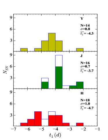
Figure 2: Distribution of $t_{1}$ for the $Y$, $J$, and $H$ light curves relative to the $B$-band maximum. The filled histograms are for SNe Ia from the CSP sample while the open histograms show the combined CSP and non-CSP sample. In the $Y$ band, we only use the objects observed by the CSP. The NIR light curves peak at within $-2$ to $-7$ d relative to the $B$ maximum.

The NIR light curves peak within $-2$ to $-7$ d of the $B$-band peak confirming the result of Folatelli2010 for SNe Ia with $\Delta m_{15}(B)$$<$1.8. There is no obvious difference between our full sample and the CSP sample as seen in the scatter. The distribution of $t_{1}$ is remarkably tight (less than one day dispersion) for all filters. This indicates a close relationship between $t^{max}_{B}$ and the NIR $t_{1}$ values for the SNe Ia in our sample.

Table 3 gives the phase of lowest scatter measured in each filter. Without any attempt to normalise the light curves, we find the smallest scatter in all NIR light curves near $t_{1}$. The dispersion remains very low for $\sim$1 week, before increasing to $>$0.2 mag at later phases.

3.3 The minimum

The minimum in $J$ occurs $\sim$2 weeks after $t^{max}_{B}$ (Fig. 3). The $Y$ light curves dip about 3 d earlier at $t_{0}=+11$ d. The minimum in $H$ is reached on average about 2 d before $J$ at $t_{0}=+12$ d. The phase range is still relatively narrow with the minima all occurring within roughly $\pm 2$ d. While $Y$ and $H$ display a tight distribution of t₀, the $J$ distribution exhibits a tail of late minima.

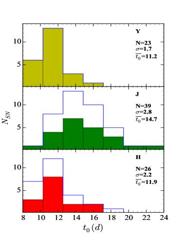
Figure 3: Distribution of $t_{0}$ in $Y$, $J$, and $H$ light curves. The $Y$ and $H$ minimum is reached a few days before the $J$ light curve dips, which occurs $\sim$2 weeks after $B$-band maximum.

Table 3: Magnitude scatter in NIR light curves. The second column indicates the time of minimum magnitude scatter in each filter, while the third column gives the scatter at this phase. The fourth column gives the phase range for which the scatter stays below 0.2 mag.

Filter	$t$	$\sigma(M)$	Phase range	SN sample
	(days)	(mag)	($\sigma(M)<0.2$ mag)
Y	$-4.4$	0.15	[$-4$ , +1]	CSP
J	$-3.6$	0.16	[$-4$ , +3]	CSP
J	$-3.8$	0.17	[$-6$ , +1]	non-CSP
H	$-5.1$	0.17	[$-5$ , +1]	CSP
H	$-4.7$	0.14	[$-7$ , +2]	non-CSP

No significant difference between the CSP and the literature samples can be seen in the distributions. The scatter among $M_{0}$ is fairly small for the three NIR bands although about 2 to 3 times larger than at t₁. In the $Y$-band, the scatter is low ($<$0.2 mag) immediately after t₀, while the $J$ and $H$ light curves display a larger dispersion at this point.

3.4 The second maximum

Figure 4 shows that t₂ occurs over a wide range of phases and can vary by as much as 20 d from one SN Ia to another. This diversity had been observed before for the $i$ light curves [e.g.][]Hamuy1996, Folatelli2010 and for $JHK$ Mandel2009, Biscardi2012. In Figure 4, we show that the mean t₂ is later in $Y$- and $J$-bands, with the $H$-band light curves reaching t₂, on average, a few days earlier. The scatter in the luminosity starts to increase slowly after t₀, and is seen to increase significantly ($>$0.5 mag) around the time of t₂ (Fig. 1).

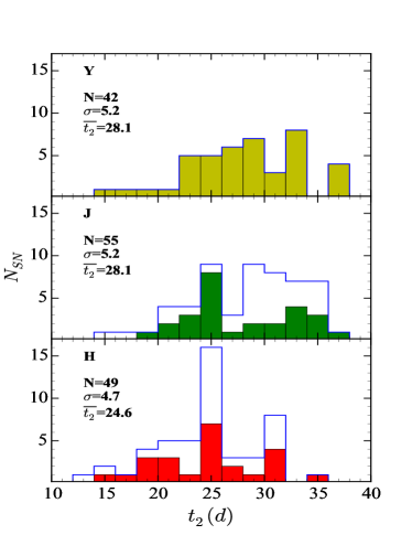
Figure 4: Distribution of t₂ in the $Y$, $J$ and $H$ light curves. Note the expanded scale on the abscissa compared to the phase ranges in Figs. 2 and 3.

3.5 The late decline

After the second maximum, the light curves steadily decline. In Fig. 5 we show the distribution of slopes calculated for SNe Ia with at least three observations in phases 40$<$$t$$<$90 d. This choice of phase range ensures that the measurements are not influenced by the second maximum. All the SNe Ia in our sample with data at these late phases come from the CSP.

There is a tight distribution of decline rates in the $Y$- and $H$-bands, with the notable exception of SN 2005M in $H$, which declined twice as fast as the other SNe Ia. The scatter in the $H$-band decline rate, when excluding SN 2005M, is only 0.004 mag per day, similar to the scatter in the $Y$ filter. The same SN is also one of the two fast declining objects in $J$ (in the fastest bin, middle panel), where the scatter in the decline rates is significantly larger than for the other two bands.

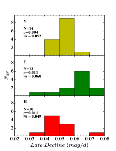
Figure 5: Distribution of decline rates after t₂.

3.6 NIR colours

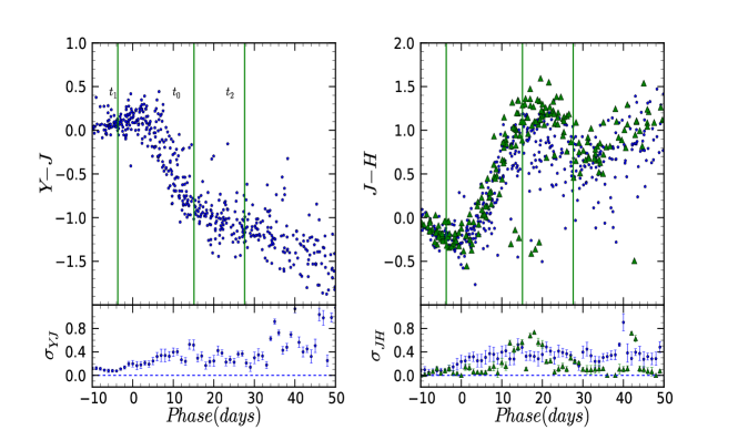
Figure 6: Left: $Y-J$ colour curve. The mean $t_{1}$, $t_{0}$ and $t_{2}$ in the $Y$ filter are plotted as green lines. The scatter plot in the lower panel only contains information from the CSP objects since the non-CSP sample does not have $Y$-filter observations. The blue points are the objects in the CSP sample, whereas the green points are the non-CSP objects. Right: $J-H$ colour curve. The epoch of minimum scatter in $J$, the average value of $t_{0}$ and $t_{2}$ in $J$ are overplotted in green. The lower panel shows the evolution of the scatter around the mean in the colour curve.

[Elias et al.1985] showed that the early $J-H$ colour evolution is rather uniform for SNe Ia. In Fig. 6, we show the colour curves ($Y-J$ and $J-H$) for the CSP and non-CSP objects. The scatter at each epoch is plotted in the lower panels. Similar to the light curves, the early colour evolution is similar for most SNe Ia in our sample.

At the first maximum the scatter is minimal in $Y-J$ ($\sigma(Y-J)=0.07$ mag) and in $J-H$ ($\sigma(J-H)=0.05$ mag). The scatter stays $<$0.1 mag between $-7$ and $-3$ d for $Y-J$ and between $-10$ and $-3$ d for $J-H$. At early times, we find that the samples display the same scatter. Immediately after the first maximum, the colour curves start to deviate like the light curves. By the time of the minimum the colours display a wide spread which continues to increase into the late decline.

The $Y-J$ colour remains fairly constant until about one week after maximum when the $Y-J$ colour starts a monotonic evolution towards bluer colours. For the $J-H$ colour, SNe Ia evolve to redder colours after maximum. Then after the light curve minimum, the $J-H$ colour tends towards slightly bluer colours until $\sim$30 d.

4 Correlations

The uniformity of the NIR light curves at maximum light suggests that the size of the surface of last scattering at these wavelengths is independent of the details of the explosion and progenitor.

A diversity in the NIR only becomes visible at later phases as the lines contributing to the line blanketing opacity arise from deeper in the ejecta. The phase and magnitude the minimum and in particular the second maximum of the NIR light curves display large variations. Correlating these changes with other SN parameters should shed light on the physical processes underlying the explosions and the release of the radiation.

In Fig. 7 we show example NIR light curves extending to late times for 10 SNe Ia in our sample. It should be noted that among these 10 SNe are two where the extinction has been determined to be high (SN 2006X and SN 2008fp). Therefore, some of the scatter can be attributed to uncorrected host galaxy extinction.

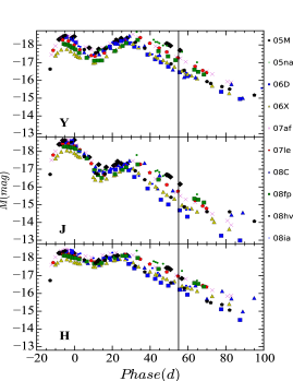
Figure 7: Complete absolute magnitude light curves in $YJH$ for the 10 objects for which a late decline is measured in all three filters. The figure illustrates that the decline rates at late times are uniform, whereas there is a large scatter in the absolute magnitude at +55 d indicated by the vertical line.

In the following sections, we note that correlations reported with $r>0.4$ are significant, and those with $r>0.65$ are termed as strong.

4.1 NIR light curve properties

In the previous section, we found a large diversity in the NIR light curve properties at post-maximum epochs. In this section, we investigate correlations between these properties in more detail. We find a correlation between $t_{0}$ and $t_{2}$ in $JH$ filters (Pearson parameter $r\sim 0.5$) suggesting that a later minimum is followed by a later second maximum. We also find a correlation between $M_{2}$ and $M_{0}$ in $Y$ and $J$ filters, with $r=0.59$ and $r=0.50$ respectively. This implies that SNe Ia with a more luminous minimum also display a more luminous second maximum.

Interestingly, the $M_{2}$ and $t_{2}$ do not correlate ($r<0.4$) in any filter. However, there we do find a significant correlation across different filters between $M_{2}$ and $t_{2}$ (e.g. $M_{2}$ in $Y$ band correlates with $t_{2}$ in $J$ band with $r=0.61$). Mandel2009 found that the rate of luminosity increase (rise rate $r/\beta$ in the Mandel2009 nomenclature) to the second maximum correlated with the luminosity of the first peak. We cannot confirm this at any significance with our data.

Comparison of Figs. 3 and 4 reveals that the light curve evolution in the $Y$-band is slowest amongst the NIR filters. SNe Ia on average reach t₀ in $Y$ earlier than in $J$ and $H$, but reach t₂ later in the $Y$ compared to the other filters. The rise time in $Y$ is nearly 4 d longer than in $J$ and nearly 7 d longer than in $H$.

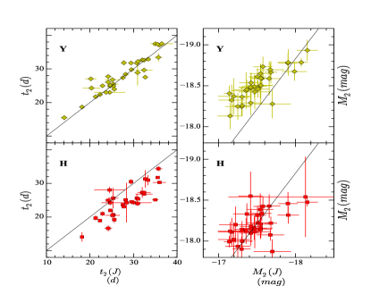
Figure 8: Phases (left) and luminosity (right) of the second maximum in NIR filters. There are clear correlations between the filters with the weakest trend in the $H$ versus $J$ luminosities. The black line is a one-to-one relation.

The phase and luminosity of the second maximum strongly correlate between the NIR filters (Fig. 8). SNe Ia with a later t₂ display a higher luminosity during the late decline. The luminosity at 55 d past the $B$ maximum, hereafter referred to as $M|_{55}$ was chosen to ensure all SNe Ia have entered the late decline well past t₂. A choice of a later phase may be more representative of the decline but would result in a smaller SN sample as not many objects are observed at these epochs and the decreasing flux results in larger uncertainties.

In Figure 9 we plot $M|_{55}$ against $t_{2}$ and $M_{2}$. A clear trend between $M|_{55}$ and $t_{2}$ is present in all filters (Pearson coefficients $r$ of 0.78, 0.92, 0.68 in the $YJH$, respectively; Fig. 9, left panels). At this phase SNe Ia are on average most luminous in $Y$ followed by $H$ and $J$, a trend that is already present at $M_{2}$. This is also reflected in the NIR colour evolution (see section §3.6).

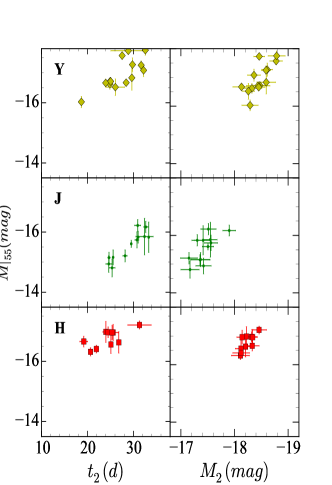
Figure 9: (Left:) Absolute magnitude at $t=55$ d in $YJH$ vs. $t_{2}$. (Right:) $M|_{55}$ compared to the absolute magnitude of the second maximum $M_{2}$.

The dispersion in $M|_{55}$ is large with $\sigma(M|_{55})=0.48$ mag, 0.51 mag and 0.30 mag in $Y$, $J$ and $H$, respectively. This is not unexpected as it continues the trend to larger (luminosity) differences in the NIR light curves with increasing phase.

4.2 Correlations with optical light curve shape parameters

It is interesting to see whether the NIR light curve parameters correlate with some of the well known optical light curve shape features [$\Delta m_{15}$;][]Burns2011.

Folatelli2010 have shown that the value of $t_{2}$ in $i$ correlated with $\Delta m_{15}(B)$. Since the dispersion increases with phase we concentrate on the second maximum and explore whether the timing and the strength correlate with the optical light curve shape.

The second maximum in the NIR is a result of an ionization transition of the Fe-group elements from doubly to singly ionized states. Models predict that $t_{2}$ depends on the amount of Ni ($M_{Ni}$) synthesized in the explosion Kasen2006. Since $M_{Ni}$ is known to correlate with $m^{max}_{B}$, which itself is a function of the light curve shape Arnett1982, Stritzinger2006, Mazzali2007, Scalzo2014, we explored the relation between $t_{2}$ and $\Delta m_{15}$ (Tab. 2).

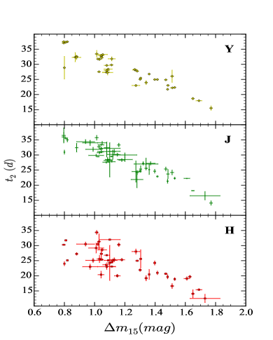
Figure 10: Comparison of t₂ in the NIR light curves with $\Delta m_{15}(B)$.

Figure 10 confirms a strong correlation between $t_{2}$ and $\Delta m_{15}$. The Pearson coefficients are 0.91, 0.93 and 0.75 for the $Y$, $J$, and $H$-bands, respectively. The weaker correlation in $H$ may be due to a low dependency on t₂ for objects with $\Delta m_{15}$ $<$ 1.2, where $t_{2}$ appears independent of $\Delta m_{15}$. This applies only to SNe Ia with a slow optical decline. For higher $\Delta m_{15}$, the trend is as strong as in the other filters.

A linear regression yields equation 1 for each filter. The RMS scatter is 2.1 d, 1.8 d and 3.0 d in the $YJH$ filters.

$$t_{2}(Y)=(-20.6\pm 1.0)\Delta m_{15}+(53.6\pm 1.2)$$ (1a)

$$t_{2}(J)=(-20.3\pm 0.9)\Delta m_{15}+(51.7\pm 1.1)$$ (1b)

$$t_{2}(H)=(-16.0\pm 2.7)\Delta m_{15}+(42.3\pm 2.8)$$ (1c)

Since the phase of the second maximum ($t_{2}$) in NIR bands is strongly correlated with $\Delta m_{15}$ and thereby the optical maximum luminosity, $t_{2}$ could also serve as an indicator of the luminosity of SNe Ia. It is noteworthy that even extreme cases, like SN 2007if, which have been associated with super-Chandrasekhar mass progenitors Scalzo2010, Scalzo2012 are fully consistent with the derived relations.

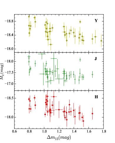
Figure 11: $M_{2}$ versus $\Delta m_{15}$ is shown and a weak correlation is observed.

There is a weak correlation between $M_{2}$ and $\Delta m_{15}$ as shown in Fig. 11, with very little difference between objects. We find $r$ values of 0.59, 0.50 and 0.63 for the $Y$, $J$, and $H$ filters, respectively.

5 Discussion

As has been shown earlier in this paper and in a number of other publications Meikle2000,WV08,BN12,Weyant2014, SN Ia NIR light curves show remarkable uniformity around maximum light, compared to at optical wavelengths. This uniformity, combined with reduced effects of extinction, holds great promise for the use of SNe Ia as distance indicators in the NIR. Kattner2012 proposed to further reduce the scatter in the luminosity of the first maximum in the NIR by a decline rate correction similar to the procedure in the optical.

The spread in optical luminosity is attributed to different masses, or distributions, of ⁵⁶Ni within the ejecta Arnett1982, Stritzinger2006, Scalzo2014. The indifference of the NIR maximum light to the nickel mass suggests that it is intermediate-mass elements that dominate the opacity in these bands at maximum light.

The NIR light curves showed an increased dispersion at later times. We attribute this increased scatter to differences in the speed of the evolution of the SNe Ia. The phase of the second maximum depends on the mass and distribution of ⁵⁶Ni, the change in opacity, the ionisation and the dominant species setting the emission.

Not all SNe Ia display a second maximum [e.g.][]Krisciunas2009 and we restricted our analysis only to objects in which the second maximum is defined well enough to be fit. This translates into a sample including only SNe Ia with $\Delta m_{15}(B)<1.8$ mag. Events without a second maximum tend to be of low luminosity, often similar to SN 1991bg, and with large $\Delta m_{15}(B)$.

The strength of the second peak in the $iJHK$ light curves does not correlate with $\Delta m_{15}$, but the phase does Folatelli2010,Biscardi2012.

As presented in the previous section, we confirm this relation between $t_{2}$ and $\Delta m_{15}$ for the $YJH$ filters. The correlation of $M_{2}$ with $\Delta m_{15}$ is rather weak (Fig. 11) although it appears somewhat stronger than in Biscardi2012 (the Pearson coefficients in our data are 0.5 and 0.63 for $J$ and $H$ compared to 0.12 and 0.08 in Biscardi2012).

5.1 A possible physical picture

The various features of the NIR light curves can be assembled into a physical picture of the explosions. The striking similarities of the late decline rates, when the SN becomes increasingly transparent to the $\gamma-$rays generated by the radioactive decays, indicate that the internal structure of the explosions is probably similar for all SNe Ia considered here. The uniform decline rates are consistent with the predictions of Woosley2007 for a range of Chandrasekhar-mass models, with different $M_{Ni}$ but similar radial distribution of iron-group elements. We find that the late-time decline rate in $J$ is faster than in $Y$ and $H$, a trend also seen between the simulated $J$ and $H$ light curves in Dessart2014. The NIR light curves depend very little on the explosion geometry Kromer2009. The DDC15 models of Blondin2013 show that the $YHK$ decline rates are similar to the pseudo-bolometric decline rate (S. Blondin, private communication). The $J$ band shows a faster decline due to a lack of emission features Spyr1994. This also explains the evolution of the $J-H$ colour curve to redder colours at late times.

At the these late times $M|_{55}$ shows a large scatter (cf. Fig. 9). If the similar late decline rates ( cf. Fig.  5) indicate a similarity in the evolution of the $\gamma$-ray escape fraction for different SNe Ia,then, a higher luminosity would translate into a higher energy input at late phases, i.e. a larger mass of Fe-group elements.

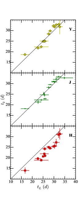
Figure 12: The phase of the second maximum versus $t_{L}$. The black line is the one-to-one relation.

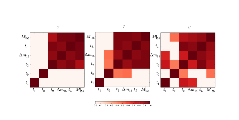
Figure 13: A summary of the correlations between the timing parameters ($t_{1}$, $t_{0}$ and $t_{2}$), $\Delta m_{15}$ , $t_{L}$ and the late time luminosity ($M|_{55}$), in each filter There is a strong correlation amongst the $t_{2}$, $\Delta m_{15}$, $t_{L}$ and $M|_{55}$ ($r>0.65$). The colorbar scales from white to red in ascending order of correlation strength. Correlations with $r<0.4$ have been set to white

Kasen2006 predicted that the second maximum should be delayed for larger Fe masses, which is exactly what is observed in the NIR [see also][]Jack2012. According to Kasen2007, the faster decline in the $B$-band light curve is mostly due to line blanketing through Fe and Co lines, which shifts the emission into the NIR and shapes the NIR light curves after maximum. The optical colour evolution post $B$-maximum is suggested to be more rapid for explosions with lower Ni masses. If this is true then the onset of the uniform $B-V$ colour evolution [referred to as the ’Lira law’ and originally defined as the uniformity of the slope of the colour curve from 30 to 90 days, although the onset is generally at earlier phase;][]Phillips1999 marks the beginning of the nebular phase. At these epochs, the SN Ia spectrum is dominated by emission lines from Fe-group elements and the emission line strength depends on the Fe mass in the explosion. We measure the time at which the SN enters the Lira law, hereafter $t_{L}$, as the epoch of inflection in the $(B-V)$ colour curve, at late times. The procedure for measuring $t_{L}$ is identical to the measurement of $t_{2}$ described in §3.4.

Figure 12 shows that $t_{2}$ coincides nearly exactly with $t_{L}$ for the $Y$ and $J$ bands. While the $H$ light curve peaks 3–4 d earlier. The reason for this is not entirely clear, but both $Y$ and $J$-bands are expected to be strongly influenced by Fe lines, while $H$ is dominated by Co lines [e.g.][]Marion2009, Jack2012. The striking coincidence of $t_{2}$ and $t_{L}$ in the NIR light curves is further evidence that $t_{2}$ directly depends on the Ni mass in the explosion.

Scalzo2014 found that the Ni mass depends on $\Delta m_{15}(B)$ and the bolometric peak luminosity. All these parameters ($m^{max}_{B}$, $\Delta m_{15}(B)$, $t_{2}$ and $t_{L}$, and NIR late-phase luminosity) can be tied to the Ni (and/or Fe) mass in the explosion. We provide a summary of the important correlations analysed in this work for the three NIR filters in Figure 13, where we correlate the timing parameters ($t_{1}$, $t_{0}$, $t_{2}$), $\Delta m_{15}$, $t_{L}$ and NIR late phase luminosity ($M|_{55}$). With most of the Fe synthesised in the explosion, we propose that all light curve parameters point to the Ni as the dominant factor in shaping the light curves. We find a consistent picture that the properties of second maximum in the NIR light curves are strongly influenced by the amount of Ni produced in the explosion followed by a more luminous decline.

The NIR colours show a pronounced evolution after t₁, the flux in the $J$ band decreases significantly with respect to both $Y$ and $H$ shortly after t₁ (Fig. 6). The reason for this depression is most likely the lack of transitions providing the required channel for radiation to emerge around 1.2 $\mu$m Spyr1994, Hoeflich1995, Wheeler1998. This persists until t₂ when the [Fe II] (1.25 $\mu$m) emission line forms and the $J$-band magnitude recovers relative to $H$, although not compared with $Y$, which is also dominated by Fe lines Marion2009. The $H$ filter is dominated by Co II lines [e.g.][]Kasen2006, Jack2012. After the second maximum $J-H$ turns redder again due to the faster decline rate in the $J$ filter.

We investigated whether the (optically) fast-declining SNe Ia can be grouped within our analysis. These SNe have very low ⁵⁶Ni mass which is almost certainly centrally located [low velocities of Fe III in the optical at late times in SN 1991bg;][]Mazzali1998 and transition so rapidly that a second maximum barely has time to form. Thus, we could not include them directly in our study. However, a comparison of $M|_{55}$ with $\Delta m_{15}(B)$ can be made for four objects of this class (SNe 2005ke, 2006mr, 2007N and 2007ax). The trend of these objects showing a fainter $M|_{55}$ luminosity with larger $\Delta m_{15}(B)$ is followed, but it is unclear whether these SN 1991bg-like SNe Ia follow the same relation as their brighter counterparts. The result remains inconclusive as the scatter remains currently too large. We note that the decline rates in the NIR at late times for these objects do not differ significantly from our sample. They follow the same distribution as in Fig 5.

5.2 Improved Distance Measurements?

The uniformity of the NIR light curves is in use for cosmological projects BN12, Weyant2014. Krisciunas2009 finds no correlation of the maximum luminosity with other light curve parameters, but identified the (optically) fast-declining SNe Ia as subluminous in the NIR compared to the other SNe Ia in their sample. In Kattner2012, the authors find a weak trend between the NIR first maximum luminosity and $\Delta m_{15}$.

We looked for NIR light curve properties to further improve SNe Ia as distance indicators. In Fig. 14 we find no significant evidence for a correlation between $M_{1}$ and $t_{2}$ for objects in our sample. The faintness of SN 2006X in this diagram is probably due to the strong absorption towards this SN.

The scatter in Fig. 1 falls to around 0.2 mag at later NIR phases. Between t₀ and t₂ all NIR light curves reach comparable luminosities. These phases are between 10 and 20 d in $Y$, near 15 and 20 d in $J$ and $H$ when SNe Ia are only about 1 (0.5) magnitude fainter than at the first maximum in $Y$ ($H$). The decline in the $J$ light curves is quite steep after the first maximum and the SNe have already faded by nearly 2 magnitudes. At least for $Y$ and $H$, it might be worthwhile to investigate whether good distances can be determined at later phases (between +10 and +15 days). The advantage would be a distance measurement with a reduced extinction component, i.e. mostly independent of the exact reddening law, and the possibility of targeted NIR observations even when the first maximum had been missed.

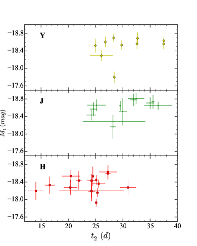
Figure 14: The magnitude of the first maximum in the $YJH$ bands is plotted against the phase of the second maximum in $J$ band. The underluminous object in $Y$ and $J$ bands is the heavily extinguished SN 2006X. In the $J$ band SN 2014J also appears fainter.

6 Conclusions

The cosmological interest in SNe Ia in the NIR stems from the small observed scatter in the peak magnitudes. We confirm this with our extended literature sample despite our simple assumptions on distances and neglect of host galaxy absorption. The phase of the first maximum in the $YJH$ light curves shows a narrow distribution. The uniformity of the SNe Ia in the NIR lasts until about one week past $B$ maximum. The NIR light curves diverge showing a large scatter by the time of the second maximum and thereafter. The IR colour curves are uniform at early phases with increasing scatter after 20 days.

These findings corroborate the use of only few IR observations near the first maximum to obtain good cosmological distances BN12, Weyant2014. The small scatter prevails for nearly a week around the first maximum and potentially another window opens near the second maximum, where the scatter again appears rather small. A condition for these measurements is accurate phase information to be able to use sparse NIR observations to derive the distances. The phase information could come from accurate optical light curves, as used here, or through spectra. The latter are needed for redshifts and classification in any case.

The information contained in the NIR light curves points towards the nickel/iron mass as the reason for the variations. The absolute magnitude 55 d past maximum together with the very uniform decline rate of the light curves in all bands, including the optical Barbon1973, Phillips1999, Leibundgut2000, points towards differences of the energy input into the ejecta with a rather uniform density structure. This is also found in theoretical studies Kasen2007,Kromer2009,Dessart2014, although most of these models employ Chandrasekhar-mass explosions and a wider range of ejecta mass models may need to be explored to confirm the similarities in the structure of the ejecta. A higher luminosity at a fixed phase in the nebular phase points towards a larger iron core and hence a higher nickel production in the explosion. A corollary is the phase of the second maximum which also occurs later for larger iron cores Kasen2006.

The strong correlation of the phase of the second IR maximum with the optical light curve shape parameter $\Delta m_{15}$ and the onset of the uniform $(B-V)$ colour evolution (‘Lira law’) point towards SNe Ia as an ordered family and nickel mass as the dominating factor in shaping the appearance of SNe Ia. With a higher nickel mass a larger Fe core is expected. This would result in higher expansion velocities observed at late phases Mazzali1998. It is worth checking whether this prediction holds true in future observations.

The phase of the second maximum should provide a handle to determining the nickel masses in SN Ia explosions, in particular for SNe Ia where absorption is significant. In cases like SN 2014J the NIR light curve can yield an independent check on the nickel mass and a direct comparison to the direct measurements of the $\gamma-$rays from the nickel decay Churazov2014, Diehl2014. A calibration of a fair set of (preferably bolometric) peak luminosities and the derived nickel masses with our parameter $t_{2}$ should lead to the corresponding relation.

We attempted to improve the IR first maximum for distance measurements and looked for a possible correlation of $M_{1}$ with the phase of the second maximum. There is a slight improvement in the $J$ band and none in $Y$ and $H$. The resulting scatter after correction in $J$ band is 0.16 mag. This is comparable to the observed value from previous studies Mandel2009, Kattner2012, Weyant2014. It remains to be seen whether larger samples will provide a better handle in the future.

Since we specifically studied the second maximum in the NIR light curves, we excluded SNe Ia, which do not display this feature. These are objects similar to either SN 1991bg, SN 2000cx or SN 2002cx and are typically faint and peculiar SNe Filippenko1992, Leibundgut1993, Li2001, Li2003, Foley2013. They appear to also display a fainter first maximum in the NIR Krisciunas2009. It would be interesting to check whether the uniform decline rate observed in the near-IR also applies to SNe Ia which do not show the second maximum. This could be used to check whether these explosions share some physical characteristics with the ones discussed here. There are only very few SNe Ia of this type and we do not find a conclusive answer. Increasing the number of SNe Ia with this information is important to assess the physical differences among the different SN Ia groups. The recent CFAIR2 catalogue Friedman2014 will provide some of these data.

The NIR light curves display a decline rate after the second maximum, which is significantly larger than the optical light curves at the same phase [e.g.][]Leibundgut2000. At very late phases ($\geq 200$ days) the near-IR light curves become nearly flat as observed for SN 2001el, while there is no observable change in the optical decline rates Stritzinger2007. It would be interesting to observe the change in decline rate between 100 and 300 days. Presumably, the internal structure of the explosions sets the transition towards the positron decays as the dominant energy source, when the ejecta have thinned enough that the $\gamma-$rays escape freely. This phase might be correlated with other physical parameters, like the nickel and ejecta mass, determined through early light curves.

A possible extension of this photometric study with detailed spectroscopic observations and theoretical spectral synthesis calculations might be worthwhile to check on the emergence of the various emission lines, trace the exact transition to the flatter IR light curves and determine whether it indicates any differences in the structure of the SNe, e.g. transition to positron channel.

Finally, Euclid will discover many SNe at near-NIR wavelengths out to cosmologically interesting redshifts [e.g.][]Astier2014. With the small scatter of the peak luminosity, these observations will provide distances with largely reduced uncertainties due to reddening. Our study confirms the promise the NIR observations of SNe Ia offer.

Appendix A Parameter Tables for the Correlations

Table 4: $Y$ filter apparent Magnitude and phase of the two maxima and the minimum for the complete sample. The phases are given in days relative to the $B$ maximum. . The full table is available online

SN	$t_{1}$	$m_{1}$	$t_{0}$	$m_{0}$	$t_{2}$	$m_{2}$
	(days)		(days)		(days)
2004eo	$-4.48\pm 0.82$	$15.90\pm 0.03$	…	…	…	…
2004ey	…	…	…	…	$31.77\pm 0.20$	$15.51\pm 0.01$
2004gs	…	…	$8.10\pm 0.76$	$17.69\pm 0.02$	$22.35\pm 0.07$	$17.16\pm 0.03$
2004gu	…	…	…	…	$37.04\pm 0.13$	$17.67\pm 0.03$
2005A	…	…	$13.70\pm 1.61$	$17.69\pm 0.41$	$27.39\pm 0.07$	$16.00\pm 0.11$

Table 5: $J$ filter apparent magnitude and phase of the two maxima and the minimum for the complete sample. The phases are given in days relative to the $B$ maximum. The full table is available online

SN	$t_{1}$	$m_{1}$	$t_{0}$	$m_{0}$	$t_{2}$	$m_{2}$
	(days)		(days)		(days)
1980N	…	…	…	…	$21.86\pm 2.70$	…
1981B	…	…	…	…	$32.19\pm 0.10$	…
1986G	…	…	…	…	$16.40\pm 1.40$	…
1998bu	…	…	…	…	$29.84\pm 0.40$	…
1999ac	…	…	…	…	$27.00\pm 2.00$	$15.61\pm 0.50$

Table 6: $H$ filter apparent magnitudes and phases of the two maxima and the minimum for the complete sample. The phases are given in days relative to the $B$ maximum. The full table is available online

SN	$t_{1}$	$m_{1}$	$t_{0}$	$m_{0}$	$t_{2}$	$m_{2}$
	(days)		(days)		(days)
1981B	…	…	…	…	$31.98\pm 0.50$	…
1986G	…	…	…	…	$12.70\pm 1.30$	$10.01\pm 0.10$
1998bu	…	…	…	…	$29.18\pm 1.65$	…
1999ee	…	…	…	…	$30.50\pm 0.70$	$15.11\pm 0.03$
2000E	…	…	…	…	$25.10\pm 0.70$	$13.85\pm 0.10$

Table 7: Late time decline rate and luminosity at +55days in $YJH$. The full table is available online

SN	slope	err	$M|_{55}$	err
	(mag/day)
Y filter
2005M	0.054	0.002	$-17.73$	0.08
2005el	0.056	0.002	$-16.72$	0.11
2005na	0.052	0.003	$-17.57$	0.13
2006D	0.050	0.001	$-16.62$	0.17
2006X	0.054	0.003	$-16.67$	0.10

Table 8: $t_{2}$ and epoch at which SN enters Lira law. The full table is available online

SN	$t_{2}$	err	$t_{L}$	err
	(days)		(days)
Y filter
2004gs	22.34	0.07	24.17	3.21
2005am	21.73	0.12	22.69	1.26
2005el	24.96	0.11	25.78	1.00
2005na	31.77	3.46	32.69	1.26
2006D	24.88	0.02	25.00	0.26

References

- [\citeauthoryearAjhar et al.2001] Ajhar E. A., Tonry J. L., Blakeslee J. P., Riess A. G., Schmidt B. P., 2001, ApJ, 559, 584
- [\citeauthoryearAmanullah et al.2014] Amanullah R., et al., 2014, ApJ, 788, 21
- [\citeauthoryearArnett1982] Arnett W. D., 1982, ApJ, 253, 785
- [\citeauthoryearAstier et al.2014] Astier P., et al., 2014, arXiv, arXiv:1409.8562
- [\citeauthoryearBarbon, Ciatti, & Rosino1973] Barbon R., Ciatti F., Rosino L., 1973, A&A, 25, 241
- [\citeauthoryearBarone-Nugent et al.2012] Barone-Nugent R. L., et al., 2012, MNRAS, 425, 1007
- [\citeauthoryearBenetti et al.2004] Benetti S., et al., 2004, MNRAS, 348, 261
- [\citeauthoryearBetoule et al.2014] Betoule M., et al., 2014, A&A, 568, 22
- [\citeauthoryearBiscardi et al.2012] Biscardi I., et al., 2012, A&A, 537, A57
- [\citeauthoryearBlondin et al.2013] Blondin S., Dessart L., Hillier D. J., Khokhlov A. M., 2013, MNRAS, 429, 2127
- [\citeauthoryearBranch & Tammann1992] Branch D., Tammann G. A., 1992, ARA&A, 30, 359
- [\citeauthoryearBurns et al.2011] Burns C. R., et al., 2011, AJ, 141, 19
- [\citeauthoryearBurns et al.2014] Burns C. R., et al., 2014, ApJ, 789, 32
- [\citeauthoryearCardelli, Clayton & Mathis1989] Cardelli J. A., Clayton G. C., Mathis J. S., 1989, ApJ, 345, 245
- [\citeauthoryearCartier et al.2014] Cartier R., et al., 2014, ApJ, 789, 89
- [\citeauthoryearChurazov et al.2014] Churazov E., et al., 2014, Natur, 512, 406
- [\citeauthoryearConley et al.2011] Conley A., et al., 2011, ApJS, 192, 1
- [\citeauthoryearContardo, Leibundgut & Vacca2000] Contardo G., Leibundgut B., Vacca W. D., 2000, A&A, 359, 876
- [\citeauthoryearContreras et al.2010] Contreras C., et al., 2010, AJ, 139, 519
- [\citeauthoryearDessart et al.2014] Dessart L., Hillier D. J., Blondin S., Khokhlov A., 2014, MNRAS, 441, 3249
- [\citeauthoryearDiehl et al.2014] Diehl R., et al., 2014, A&A, submitted (arXiv:1409.5477)
- [\citeauthoryearElias et al.1981] Elias J. H., Frogel J. A., Hackwell J. A., Persson S. E., 1981, ApJ, 251, L13
- [\citeauthoryearElias & Frogel1983] Elias J. H., Frogel J. A., 1983, ApJ, 268, 718
- [\citeauthoryearElias et al.1985] Elias J. H., Matthews K., Neugebauer G., Persson S. E., 1985, ApJ, 296, 379
- [\citeauthoryearElias-Rosa et al.2006] Elias-Rosa N., et al., 2006, MNRAS, 369, 1880
- [\citeauthoryearFilippenko et al.1992] Filippenko A. V., et al., 1992, AJ, 104, 1543
- [\citeauthoryearFolatelli et al.2010] Folatelli G., et al., 2010, AJ, 139, 120
- [\citeauthoryearFoley et al.2013] Foley R. J., et al., 2013, ApJ, 767, 57
- [\citeauthoryearFoley et al.2014] Foley R. J., et al., 2014, MNRAS, 443, 2887
- [\citeauthoryearFreedman et al.2001] Freedman W. L., et al., 2001, ApJ, 553, 47
- [\citeauthoryearFreedman et al.2009] Freedman W. L., et al., 2009, ApJ, 704, 1036
- [\citeauthoryearFriedman et al.2014] Friedman A. S., et al., 2014, arXiv, arXiv:1408.0465
- [\citeauthoryearGoobar & Leibundgut2011] Goobar A., Leibundgut B., 2011, ARNPS, 61, 251
- [\citeauthoryearGoobar et al.2014] Goobar A., et al., 2014, ApJ, 784, L12
- [\citeauthoryearGuy et al.2010] Guy J., et al., 2010, A&A, 523, A7
- [\citeauthoryearGuy et al.2007] Guy J., et al., 2007, A&A, 466, 11
- [\citeauthoryearGuy et al.2005] Guy J., Astier P., Nobili S., Regnault N., Pain R., 2005, A&A, 443, 781
- [\citeauthoryearHamuy et al.1996] Hamuy M., Phillips M. M., Suntzeff N. B., Schommer R. A., Maza J., Smith R. C., Lira P., Aviles R., 1996, AJ, 112, 2438
- [\citeauthoryearHöflich, Khokhlov & Wheeler1995] Höflich P., Khokhlov A., Wheeler C., 1995, ASPC, 73, 441
- [\citeauthoryearJack, Hauschildt, & Baron2012] Jack D., Hauschildt P. H., Baron E., 2012, A&A, 538, A132
- [\citeauthoryearJensen et al.2003] Jensen J. B., Tonry J. L., Barris B. J., Thompson R. I., Liu M. C., Rieke M. J., Ajhar E. A., Blakeslee J. P., 2003, ApJ, 583, 712
- [\citeauthoryearJha, Riess, & Kirshner2007] Jha S., Riess A. G., Kirshner R. P., 2007, ApJ, 659, 122
- [\citeauthoryearKasen2006] Kasen D., 2006, ApJ, 649, 939
- [\citeauthoryearKasen & Woosley2007] Kasen D., Woosley S. E., 2007, ApJ, 656, 661
- [\citeauthoryearKattner et al.2012] Kattner S., et al., 2012, PASP, 124, 114
- [\citeauthoryearKrisciunas et al.2001] Krisciunas K., et al., 2001, AJ, 122, 1616
- [\citeauthoryearKrisciunas et al.2003] Krisciunas K., et al., 2003, AJ, 125, 166
- [\citeauthoryearKrisciunas et al.2004] Krisciunas K., et al., 2004a, AJ, 127, 1664
- [\citeauthoryearKrisciunas et al.2004] Krisciunas K., et al., 2004b, AJ, 128, 3034
- [\citeauthoryearKrisciunas et al.2007] Krisciunas K., et al., 2007, AJ, 133, 58
- [\citeauthoryearKrisciunas et al.2009] Krisciunas K., et al., 2009, AJ, 138, 1584
- [\citeauthoryearKromer & Sim2009] Kromer M., Sim S. A., 2009, MNRAS, 398, 1809
- [\citeauthoryearLeaman et al.2011] Leaman J., Li W., Chornock R., Filippenko A. V., 2011, MNRAS, 412, 1419
- [\citeauthoryearLeibundgut1988] Leibundgut B., 1988, PhD thesis, University of Basel
- [\citeauthoryearLeibundgut2000] Leibundgut B., 2000, A&ARv, 10, 179
- [\citeauthoryearLeibundgut et al.1993] Leibundgut B., et al., 1993, AJ, 105, 301
- [\citeauthoryearLeloudas et al.2009] Leloudas G., et al., 2009, A&A, 505, 265
- [\citeauthoryearLi et al.2001] Li W., et al., 2001, PASP, 113, 1178
- [\citeauthoryearLi et al.2003] Li W., et al., 2003, PASP, 115, 453
- [\citeauthoryearLira1996] Lira P., 1996, MsT, 3
- [\citeauthoryearMaeda et al.2010] Maeda K., Taubenberger S., Sollerman J., Mazzali P. A., Leloudas G., Nomoto K., Motohara K., 2010, ApJ, 708, 1703
- [\citeauthoryearMaeda et al.2011] Maeda K., et al., 2011, MNRAS, 413, 3075
- [\citeauthoryearMaguire et al.2012] Maguire K., et al., 2012, MNRAS, 426, 2359
- [\citeauthoryearMarion et al.2009] Marion G. H., Höflich P., Gerardy C. L., Vacca W. D., Wheeler J. C., Robinson E. L., 2009, AJ, 138, 727
- [\citeauthoryearMandel et al.2009] Mandel K. S., Wood-Vasey W. M., Friedman A. S., Kirshner R. P., 2009, ApJ, 704, 629
- [\citeauthoryearMargutti et al.2014] Margutti R., Parrent J., Kamble A., Soderberg A. M., Foley R. J., Milisavljevic D., Drout M. R., Kirshner R., 2014, ApJ, 790, 52
- [\citeauthoryearMazzali et al.1997] Mazzali P. A., Chugai N., Turatto M., Lucy L. B., Danziger I. J., Cappellaro E., della Valle M., Benetti S., 1997, MNRAS, 284, 151
- [\citeauthoryearMazzali et al.1998] Mazzali P. A., Cappellaro E., Danziger I. J., Turatto M., Benetti S., 1998, ApJ, 499, L49
- [\citeauthoryearMazzali et al.2007] Mazzali P. A., Röpke F. K., Benetti S., Hillebrandt W., 2007, Sci, 315, 825
- [\citeauthoryearMatheson et al.2012] Matheson T., et al., 2012, ApJ, 754, 19
- [\citeauthoryearMeikle2000] Meikle W. P. S., 2000, MNRAS, 314, 782
- [\citeauthoryearNobili et al.2005] Nobili S., et al., 2005, A&A, 437, 789
- [\citeauthoryearNobili & Goobar2008] Nobili S., Goobar A., 2008, A&A, 487, 19
- [\citeauthoryearPastorello et al.2007] Pastorello A., et al., 2007, MNRAS, 377, 1531
- [\citeauthoryearPeacock et al.2006] Peacock J. A., Schneider P., Efstathiou G., Ellis J. R., Leibundgut B., Lilly S. J., Mellier Y., 2006, ESA and ESO, Report on the ESA-ESO Working Group on Fundamental Cosmology (arXiv:astro-ph/0610906)
- [\citeauthoryearPerlmutter et al.1999] Perlmutter S., et al., 1999, ApJ, 517, 565
- [\citeauthoryearPhillips1993] Phillips M. M., 1993, ApJ, 413, L105
- [\citeauthoryearPhillips2012] Phillips M. M., 2012, PASA, 29, 434
- [\citeauthoryearPhillips et al.1999] Phillips M. M., Lira P., Suntzeff N. B., Schommer R. A., Hamuy M., Maza J., 1999, AJ, 118, 1766
- [\citeauthoryearPhillips et al.2006] Phillips M. M., et al., 2006, AJ, 131, 2615
- [\citeauthoryearPhillips et al.2013] Phillips M. M., et al., 2013, ApJ, 779, 38
- [\citeauthoryearPignata et al.2008] Pignata G., et al., 2008, MNRAS, 388, 971
- [\citeauthoryearPinto & Eastman2000] Pinto P. A., Eastman R. G., 2000, ApJ, 530, 757
- [\citeauthoryearRiess, Press, & Kirshner1996] Riess A. G., Press W. H., Kirshner R. P., 1996, ApJ, 473, 88
- [\citeauthoryearRiess et al.1998] Riess A. G., et al., 1998, AJ, 116, 1009
- [\citeauthoryearScalzo et al.2010] Scalzo R., et al., 2010, ApJ, 713, 1073
- [\citeauthoryearScalzo et al.2012] Scalzo R., et al., 2012, ApJ, 757, 12
- [\citeauthoryearScalzo et al.2014] Scalzo R., et al., 2014, MNRAS, 560
- [\citeauthoryearScolnic et al.2014] Scolnic D. M., Riess A. G., Foley R. J., Rest A., Rodney S. A., Brout D. J., Jones D. O., 2014, ApJ, 780, 37
- [\citeauthoryearSpyromilio, Pinto, & Eastman1994] Spyromilio J., Pinto P. A., Eastman R. G., 1994, MNRAS, 266, L17
- [\citeauthoryearStritzinger & Sollerman2007] Stritzinger M., Sollerman J., 2007, A&A, 470, L1
- [\citeauthoryearStritzinger et al.2006] Stritzinger M., Leibundgut B., Walch S., Contardo G., 2006, A&A, 450, 241
- [\citeauthoryearStritzinger et al.2011] Stritzinger M. D., et al., 2011, AJ, 142, 156
- [\citeauthoryearTonry et al.2001] Tonry J. L., Dressler A., Blakeslee J. P., Ajhar E. A., Fletcher A. B., Luppino G. A., Metzger M. R., Moore C. B., 2001, ApJ, 546, 681
- [\citeauthoryearTripp1998] Tripp R., 1998, A&A, 331, 815
- [\citeauthoryearTully1988] Tully R. B., 1988, Nearby Galaxies Catalog, Cambridge: University Press
- [\citeauthoryearValentini et al.2003] Valentini G., et al., 2003, ApJ, 595, 779
- [\citeauthoryearWeyant et al.2014] Weyant A., Wood-Vasey W. M., Allen L., Garnavich P. M., Jha S. W., Joyce R., Matheson T., 2014, ApJ, 784, 105
- [\citeauthoryearWheeler et al.1998] Wheeler J. C., Höflich P., Harkness R. P., Spyromilio J., 1998, ApJ, 496, 908
- [\citeauthoryearWillick et al.1997] Willick J. A., Courteau S., Faber S. M., Burstein D., Dekel A., Strauss M. A., 1997, ApJS, 109, 333
- [\citeauthoryearWood-Vasey et al.2008] Wood-Vasey W. M., et al., 2008, ApJ, 689, 377
- [\citeauthoryearWoosley et al.2007] Woosley S. E., Kasen D., Blinnikov S., Sorokina E., 2007, ApJ, 662, 487
- [\citeauthoryearWoosley & Weaver1986] Woosley S. E., Weaver T. A., 1986, ARA&A, 24, 205