Impact of microphysics on the growth of one-dimensional breath figures

Abstract

Droplet patterns condensing on solid substrates (breath figures) tend to evolve into a self-similar regime, characterized by a bimodal droplet size distribution. The distributions comprise a bell-shaped peak of monodisperse large droplets, and a broad range of smaller droplets. The size distribution of the latter follows a scaling law characterized by a non-trivial polydispersity exponent. We present here a numerical model for three-dimensional droplets on a one-dimensional substrate (fiber) that accounts for droplet nucleation, growth and merging. The polydispersity exponent retrieved using this model is not universal. Rather it depends on the microscopic details of droplet nucleation and merging. In addition, its values consistently differ from the theoretical prediction by Blackman (Phys. Rev. Lett., 2000). Possible causes of this discrepancy are pointed out.

I Introduction

When a flux of supersaturated vapor gets into contact with a solid substrate, a condensation process can originate, leading to the formation of droplets patterns on the substrate (“breath figures” Rayleigh (1911)). The interest for breath figures is both theoretical and practical. From the theoretical point of view, they can be used as a test ground for scaling concepts in a well-posed non-equilibrium setting. From the practical point of view, they appear in many natural phenomena, e.g. dew deposition on a spider net or on a leaf. They can also be exploited for technological applications: water collection from dew harvesting Nikolayev et al. (1996); Clus et al. (2008); Lekouch et al. (2011), biological sterilization Beysens (2006), manufacturing of surface structures and patterns for nano-technologies Böker et al. (2004); Haupt et al. (2004); Wang et al. (2007); Rykaczewski et al. (2011), fabrication of efficient heat-exchangers and cooling devices Sikarwar et al. (2011); Rose (2002); Leach et al. (2006). For such applications, understanding and controlling the droplets formation, growth and coalescence is crucial.

The formation of breath figures undergoes several phases Beysens et al. (1991). First, the droplets nucleate on the substrate; then they grow and coalesce, creating a roughly monodisperse distribution. Eventually the space released by merging is sufficient for the nucleation of new droplets. As the evolution continues, self-similar droplet patterns appear Viovy et al. (1988); Family and Meakin (1988); Kolb (1989); Brilliantov et al. (1998).

In this phase, bimodal droplet size distributions emerge in experiments Beysens and Knobler (1986); Viovy et al. (1988); Carlow et al. (1997); Haderbache et al. (1998); Blaschke et al. (2012), as well as in simulations Family and Meakin (1989a); Ulrich et al. (2004); Blaschke et al. (2012). The size distributions feature a monodisperse bell-shaped peak for the largest droplets, and a power-law distribution for the smaller droplets, characterized by a non-trivial polydispersity exponent. Scaling descriptions for the droplet number density have been largely adopted in the classical theory for breath figures Viovy et al. (1988); Family and Meakin (1988, 1989a, 1989b); Meakin and Family (1988); Meakin (1991, 1992). Such a theory relates the polydispersity exponent to the exponents for the time decay of the droplet number and the porosity, i.e. the fraction of the non-wetted area over the total area of the substrate Kolb (1989); Brilliantov et al. (1998). The scaling descriptions of the droplet size distribution are also solutions Cueille and Sire (1997, 1998) of the Smoluchowski coagulation equation Smoluchowski (1916), an integro-differential equation describing the evolution of the droplet size distribution as a consequence of merging processes. However, for droplets growing on two-dimensional substrates the polydispersity exponent derived from the solution of the Smoluchowski coagulation equation Blackman and Brochard (2000) was found to be noticeably smaller than the value found in numerical simulations Blaschke (2010); Blaschke et al. (2012) and larger than the one observed in experiments Blaschke et al. (2012).

In the present paper, we examine the case of a one-dimensional substrate with three-dimensional droplets. We use a numerical approach in order to test the existing scaling theory and, in particular, the common assumption that the polydispersity exponent takes a universal value Viovy et al. (1988); Family and Meakin (1988, 1989a, 1989b); Meakin and Family (1988); Meakin (1991, 1992); Blackman and Brochard (2000). We introduce a numerical model based on a nucleation rule governed by surface tension-driven instabilities. The dynamics account for the presence of a precursor film between droplets, droplet growth due both to direct mass deposition from the surrounding vapor and surface diffusion, and non-trivial droplet interactions due to deviations from the spherical shape. By means of simulations, we systematically explore the dependence of the droplet patterns on the deposition rate, the rules of droplet interaction, the radius of the fiber and the nucleation radius. Surprisingly, we find a dependence of the polydispersity exponent of the droplet size distribution on the microscopic details of the model, leading to the conclusion that the polydispersity exponent is not universal, as assumed in the classical scaling models. Moreover, we observe a sizable mismatch between the predicted Blackman and Brochard (2000) and the observed values of polydispersity exponent. We point out possible sources of the discrepancies.

The paper is organized as follows. In Sect. II we introduce our model and its numerical implementation. In Sect. III we revisit the scaling description of breath figures with special emphasis on the predictions for droplet growth on fibers. These predictions are then, in Sect. IV, carefully tested by comparison to comprehensive numerical data. Finally, we conclude in Sect. V.

II Model and numerical method

The precise dynamics of droplet nucleation and growth on a solid substrate is still a debated matter and depends on the specific system. Possible mechanisms include Beysens et al. (1991); Beysens (2006) heterogeneous nucleation on impurities and defects of the substrate, homogeneous nucleation, hydrodynamic instabilities, surface diffusion on the substrate, direct condensation of the vapor molecules on the droplets surface, coalescence with neighboring droplets, heat transfer localized at the triple line and preventing nucleation. The radius of an isolated droplet on a substrate increases following a power law in time, whose exponent changes according to the specific growth mechanism Rose and Glicksman (1973); Beysens et al. (1991); Ucar and Erbil (2012). However, in densely populated droplets systems, the growth is always dominated by coalescence. Therefore, the growth exponent of the average radius depends only on the dimensionalities of the droplets and the substrate Family and Meakin (1988).

II.1 Modeling breath figures on a fiber

We model breath figures on a fiber as a one-dimensional chain of spherical droplets, in contact with a supersaturated vapor. The $i^{th}$ droplet has a radius $R_{i}$ and an interaction range $\varepsilon R_{i}$, where $\varepsilon$ is constant for all the droplets. Such an interaction range has been introduced to keep into account the deviation from the spherical shape observed in experiments McHale and Newton (2002) (see Fig. 1). We account for a cylindrical water prewetting film surrounding the fiber, in the spaces between the droplets. Water is deposited on the fiber by condensation from the surrounding vapor. We do not consider removal of water from the fiber by evaporation and gravity.

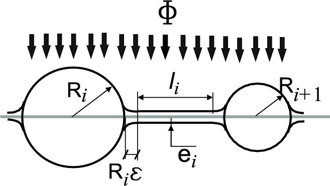
Figure 1: Sketch of the model adopted for the numerical simulation of the growth of droplets $i$ and $i+1$ with radii $R_{i}$ and $R_{i+1}$, respectively. The droplets reside on a fiber (solid gray line). They grow due to a constant water flux per unit length, $\Phi$ [$\mu$m²s^-1], due to the supersaturated vapor impinging on the fiber. There is a precursor film of radial thickness $e_{i}$ in the region between adjacent droplets, which has a length $l_{i}$. When the precursor film collects sufficient water volume, new droplets are nucleated. When two droplets approach each other within their interaction ranges $\varepsilon R_{i}$ and $\varepsilon R_{i+1}$, they merge.

We consider a case where the supersaturation of the vapor is small and the diffusive transport to the thread is the growth limiting process for the droplets. In this case we expect cylindrically symmetric vapor concentration profiles in the far field. We assume that the system is in thermal steady-state conditions, i.e. the water flux deposited on the fiber $\Phi$ – water volume per unit length per unit time – is small enough to keep the temperature of the droplets and the fiber uniform and invariant in time. We also assume hydrodynamic steady-state conditions, taking $\Phi$ to be constant in time and independent of the position, $x$, on the fiber. These approximations have been largely adopted in the study of breath figures Viovy et al. (1988) and can be considered reasonable for laminar vapor flows. The modelling of more complicated vapor flows may require the inclusion of correction terms, but this is beyond the scope of the present paper.

II.2 Evolution of the droplets

We adopt an event-driven approach and periodic boundary conditions for the fiber. In order to simplify the problem, we decouple the treatment of the droplets growth due to the impinging flux from the nucleation process. In particular, for each time step, we consider the growth in a time-continuous fashion and the nucleation in a time-discrete fashion. The algorithm to advance from time $t_{j}$ to the next instant $t_{j+1}$ proceeds as follows. At first, we only consider the droplets growth due to the water flux impinging on the droplets themselves and we disregard the nucleation of new droplets. The constant flux density $\Phi$ impinging on a length $2R_{i}$ covered on the fiber by the particle $i$ results in a growth law

$$\frac{d{}}{d{t}}\left(\frac{4}{3}\pi R_{i}^{3}\right)=2R_{i}\Phi$$ (1)

We integrate Eq. (1) in time, from $t$ to $t+\Delta t$, finding

$$R_{i}(t+\Delta t)=\sqrt{\frac{\Phi\Delta t}{\pi}+R_{i}^{2}(t)}\,.$$ (2)

We calculate the time intervals $\Delta t_{i}$ for binary merging events between adjacent droplets $i$ and $i+1$, by solving the system

$$x_{i+1}-x_{i}=(1+\varepsilon)\left[R_{i+1}(t+\Delta t_{i})+R_{i}(t+\Delta t_{i})\right]$$ (3)

where $x_{i}$ and $x_{i+1}$ are the positions of the respective centers (note that they only move when the droplets merge). We take the minimum of these time intervals, $\Delta t_{\text{merge}}=\min{\Delta t_{i}}$, as a first estimate of the time step to advance the system in time. This time step corresponds to the first merging event that would take place if there was no nucleation and no water deposited between the droplets. We calculate the volume of water $V_{\text{gap},i}$ deposited on the gaps between adjacent droplets $i$ and $i+1$ during the time $\Delta t_{\text{merge}}$, by integrating

$$\frac{d{V_{\text{gap},i}}}{d{t}}=\Phi[x_{i+1}-x_{i}-R_{i+1}-R_{i}]$$ (4)

between $t$ and $t+\Delta t_{\text{merge}}$.

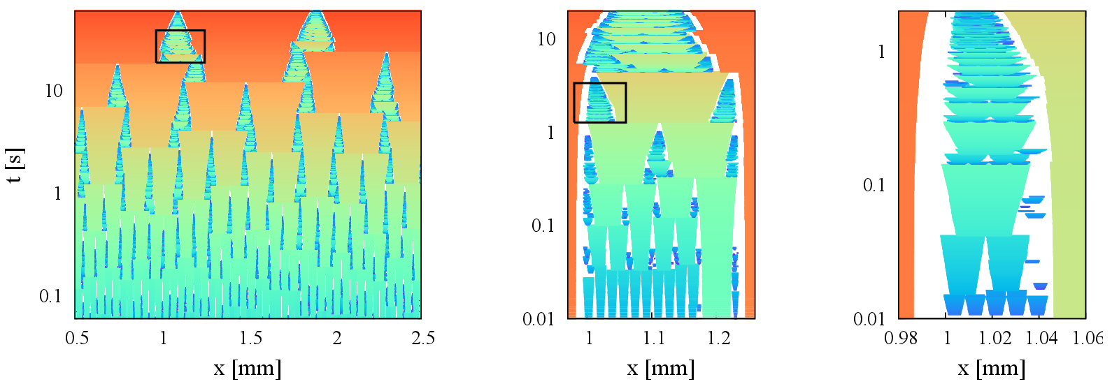
Figure 2: (Color online.) Time evolution of the space occupied by the droplets for $\varepsilon=2\%$, $\Phi=1000\,\mu$m${}^{2}/$s, $N_{0}=1.5\times 10^{5}$, and $R_{f}=R_{\text{min}}=1\,\mu$m. The different colors represent the different ages of the droplets at the considered time instant and they vary from dark (blue online), for the youngest and still very small droplets to lit-gray (yellow, then red online), for the oldest hence largest droplets. The central panel is a magnification of the area indicated by the black frame in the left panel, and the right panel shows a magnification of the frame in the central panel. They are both displayed on a logarithmic scale with the origin corresponding to the instant when the free area started to be populated (i.e. the bottom side of the black frame in the previous panel).

II.3 Nucleation of droplets

In each time step we determine if one or more nucleation events could happen during the time interval $\Delta t_{\text{merge}}$. To this aim, we consider the existence of a cylindrical precursor film, surrounding the parts of the fiber where no droplets are present. The precursor film grows in time by deposition of mass and may eventually develop into a surface tension-driven instability. Stability analysis de Gennes et al. (2004) for a fiber of radius $R_{f}$ reveals that perturbations with a wavelength $\lambda>2\pi R_{f}$ are unstable. The most unstable perturbation, i.e. the fastest growing perturbation, has a wavelength $\lambda^{*}=2\sqrt{2}\pi R_{f}$ de Gennes et al. (2004). Therefore, $\lambda^{*}$ can be regarded as a characteristic wavelength of the system. Necklace-shaped chains of droplets have been observed in experiments on fibers, where equispaced droplets appeared at a distance $\lambda^{*}$ from each other de Gennes et al. (2004). In our model, we consider that a nucleation event can take place between two droplets $i$ and $i+1$, during the time $\Delta t_{\text{merge}}$ only if the gap length $l_{i}$ between such droplets, is larger than the characteristic wavelength of the first unstable perturbation $\lambda^{*}$. The gap length is defined as $l_{i}(t)=x_{i+1}-x_{i}-(1+\varepsilon)(R_{i+1}+R_{i})$ and, in order to have a nucleation event, it has to be

$$l_{i}>\lambda^{*}=2\sqrt{2}\pi R_{f}$$ (5)

From the length of the gap $l_{i}$, we determine the number of possible equispaced nucleation sites in the gap, $N_{i}=\lfloor l_{i}/\lambda^{*}\rfloor$. Additionally, we impose a minimum droplet size $R_{\text{min}}$, for the nucleation event to take place. We approximate the film between the droplets $i$ and $i+1$ as a cylinder with volume

$$V_{\text{film},i}=\pi\left[(R_{f}+e_{i})^{2}-R_{f}^{2}\right]l_{i}\,,$$ (6)

where $e_{i}$ is the thickness of the film. We check if the amount of liquid $V_{\text{gap},i}$ deposited in the gap $l_{i}$ during the time $\Delta t_{\text{merge}}$ is large enough to satisfy the following condition:

$$V_{\text{film},i}=V_{\text{film},i}^{0}+V_{\text{gap},i}\geq\frac{4}{3}\pi R_{\text{min}}^{3}N_{i}\,,$$ (7)

where $V_{\text{film},i}^{0}$ is the volume of the precursor film in the $i^{th}$ gap at the beginning of the time step $\Delta t_{\text{merge}}$, and $V_{\text{gap},i}$ is derived by integrating Eq. (4) over $\Delta t_{\text{merge}}$. In nucleation processes, the critical droplet radius required to have a nucleation site can be calculated as Butt et al. (2003) $R_{\text{nucl}}={2\sigma}/\left[{\rho_{L}R_{V}T\textmd{ln}(p_{V}/p_{\infty})}\right]$, in which $\sigma$ is the surface tension between the liquid and the vapor, $\rho_{L}$ is the density of the liquid, $T$ is the temperature expressed in Kelvin, $R_{V}$ is the universal gas constant for water vapor, $p_{V}/p_{\infty}$ is the supersaturation rate, with $p_{V}$ the pressure of the vapor and $p_{\infty}$ the pressure of the saturated vapor. In our model we adopt the minimum droplet size as $R_{\text{min}}=R_{\text{nucl}}$. For typical environmental temperatures ($20$ – $40^{\circ}\text{C}$) and supersaturation rates $p_{V}/p_{\infty}\geq 1.001$ we have $R_{\text{nucl}}<1\,\mu$m. If Eq. (5) and Eq. (7) are both satisfied, a new nucleation event takes place. If Eq. (5) is satisfied but Eq. (7) is not, we consider the volume of water $V_{\text{gap},i}$ deposited on the $i^{th}$ gap as increasing the thickness of the cylindrical precursor film, and we store the information until the next time step. If neither Eq. (5) nor Eq. (7) are satisfied, we consider the amount of water deposited on the gap $V_{\text{gap},i}$ as collected by the droplets adjacent to the bridge itself. In particular, this water volume will be collected by the largest droplet, due to the Laplace pressure $p_{L}$ de Gennes et al. (2004). Such a pressure depends on the local curvature and, in the case of a spherical droplet of radius $R$, it is given by $p_{L}=2\sigma/R$.

II.4 Merging of droplets

We advance the system in time, by evolving it accordingly to the estimated $\Delta t_{\text{merge}}$: we grow the droplets, we insert the new nucleated ones and we merge the droplets when they approach each other within their interaction ranges. In order to do so, we replace the two merging droplets with a new one, with a mass equal to the sum of the masses of the merging ones. Its center is located in the center of mass of the two droplets. In the simulation we explicitly prevent triple merging events between neighboring droplets. Though rare, such unphysical events could occur in the described numerical scheme, due to the collection of liquid from the adjacent water bridges. When triple merging is at hand at the end of the estimated time step $\Delta t_{\text{merge}}$, we halve the estimated time step, and we evolve the system accordingly.

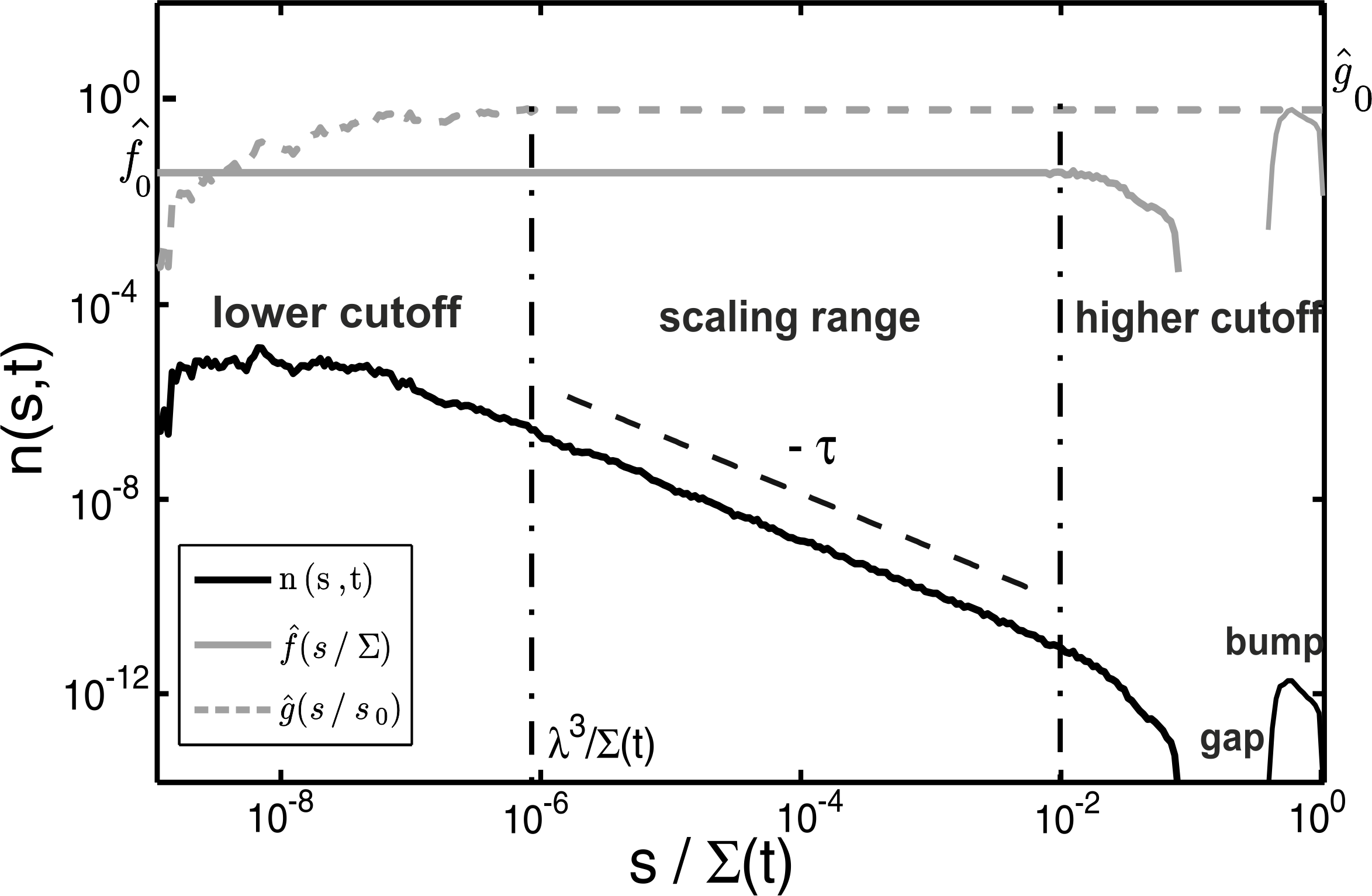
Figure 3: Droplet number density for $\varepsilon=2\%$, $R_{f}=R_{\text{min}}=1\,\mu$m, $\Phi=1000\,\mu$m${}^{2}/$s, $L_{f}$ = 1 m, $N_{0}=1.5\times 10^{5}$. The solid black line represents $n(s,t)$. The dashed black line is a fitting line for the polydisperse scaling range of the droplets and it has a slope $-\tau$ on the log-log scale. The gray solid line represents the cutoff for the large droplets $\hat{f}(s/\Sigma(t))$. The gray dashed line represents the cutoff for the small droplets: $\hat{g}(s/s_{0})$. The two vertical dash-dotted lines delimit the scaling range. For small droplets ($s<\lambda^{*}$) the distribution is dominated by $\hat{g}(s/s_{0})$. For large droplets ($s/\Sigma(t)>1\%$), the distribution is dominated by $\hat{f}(s/\Sigma(t))$. In this range, we can identify a monodisperse bump, corresponding to the oldest droplets, and a gap, corresponding to the times where the spaces released by merging droplets were not large enough to allow the nucleation of new droplets. The present graphs are derived by averaging the droplet size distributions over 10 time instants and over five simulations with different but equivalent initial conditions. The considered instants are in the self-similar regime ($t>1000$ s) and they are chosen in such a way to have 100 points per time decade.

III Scaling theory for droplets on a fiber

In Fig. 2 we show the time evolution of the droplets and their coverage of the fiber surface. The horizontal colored segments represent the areas covered by the droplets on the fiber at a certain time $t$. Different colors reflect the different ages of the droplets at the specific time $t$. In black (blue online) we represent newly created small droplets, and the color fades (turning to yellow, then red online) as the droplets become older. When two droplets merge, they release two regions of length $\sim R_{1}+R_{2}-\left(R_{1}^{3}+R_{2}^{3}\right)^{1/3}$. For sufficiently big droplets the released space is large enough to host new droplets. The opening gaps become larger with the increase of the largest droplets. Eventually, new droplets nucleate and grow in the gaps, forming a hierarchical structure in the droplet size distribution. After a sufficiently long time, self-similar droplet patterns emerge: pictures taken at different time instants look alike, apart from length rescaling (cf. Fig. 2). This is reflected in a power-law size distribution of the middle-sized droplets Family and Meakin (1988, 1989a, 1989b); Meakin and Family (1988); Meakin (1991, 1992), characterized by an exponent $\tau$ (see Fig. 3), namely the polydispersity exponent. On the other hand, the largest (oldest) and the smallest (newest) droplets have a different behavior. Their physics is captured in cutoff functions which describe the termination of the power law for large and small droplets. Blaschke et al. (2012). The small-scale cutoff accounts for the minimum droplet size $R_{\text{min}}$ and the characteristic length of the surface tension-driven instability in the precursor film $\lambda^{*}$. The large-scale cutoff comprises a bump and a gap (see Fig. 3). The bump represents the oldest droplets in the system (first droplet population). The gap originates from the times where the openings generated between the first droplets were still too small to admit a second wave of nucleation.

III.1 Size of the largest droplets

We consider the following simplified setting, in order to give an estimate of the growth law in time of the largest droplet size $\Sigma(t)$. At time $t_{n}$, we take a chain of monodisperse droplets of radius $R_{n}$ and size $\Sigma(t_{n})=R_{n}^{3}$, in contact with each other (see Fig. 4). At time $t_{n}^{*}$, the droplets have merged two by two, therefore $\Sigma(t_{n}^{*})=2\Sigma(t_{n})$. Since the merging process is almost instantaneous, $t_{n}^{*}\simeq t_{n}$. After merging, the droplets start to grow as an effect of the deposition of a uniform water flux per unit length, $\Phi$, on the fiber. Due to mass conservation, at times $t_{n}$ and $t_{n+1}$, it must be $2R\Phi t=\frac{4}{3}\pi R^{3}$. Hence,

$$\Sigma=\left(\frac{3\Phi}{2\pi}\right)^{3/2}t^{z}\ \ \mbox{ with }z=3/2\,.$$ (8)

The so-calculated exponent $z$ is in agreement with both experimental findings Steyer et al. (1990) and theoretical predictions Family and Meakin (1988). The prefactor $\left(\frac{3\Phi}{2\pi}\right)^{3/2}$ has to be regarded as a lower bound. Since the merging is assumed to happen instantaneously, the largest droplet in the system at time $t_{n}^{*}\simeq t_{n}$ will most likely be a droplet that has just originated from a merging. Hence, the upper bound for the prefactor will be $2\left(\frac{3\Phi}{2\pi}\right)^{3/2}$.

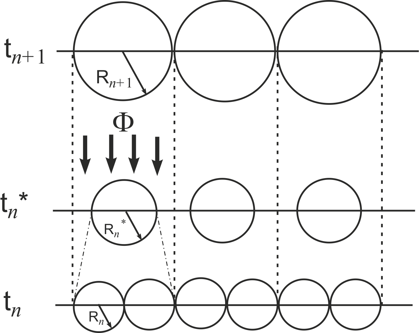
Figure 4: Sketch of the simplified model adopted for deriving the time growth law of the size of the largest droplet $\Sigma(t)$. The exponent of such a time growth is calculated based on the assumptions that the droplets are monodisperse and in touch with each other. The considered mechanisms governing the growth are the droplet coalescence two by two and the deposition of water from a uniform external flux per unit length $\Phi$.

III.2 The droplet number density $n(s,t)$

The droplet number density $n(s,t)$ is defined as the number of droplets of size $s$ at time $t$ per size interval $\text{d}s$ of droplets and unit length of the substrate, where $s=r^{3}$ is the size of a droplet with radius $r$. In our case, $n(s,t)$ has the units of $[m]^{-4}$. Consequently, the Buckingham-Pi theorem Barenblatt (2003) ensures that the droplet number density can be expressed as $n(s,t)=s^{-\theta}f(s/\Sigma(t),s/s_{0})$, where $f(x)$ is a dimensionless scaling function, $s_{0}$ characterizes the cutoff for the small droplets, $\Sigma(t)$ is the maximum droplet size at time $t$, and $\theta=(D+d)/D$ Family and Meakin (1989a) is an exponent depending on the dimensionality of the droplets $D$ and of the substrate $d$. Here, we consider the case of three-dimensional droplets, $D=3$, growing on a one-dimensional fiber, $d=1$. Therefore, from merely dimensional considerations one infers that $\theta=4/3$.

The classical scaling theory for breath figures Family and Meakin (1988, 1989a) established that, in the late regime, the droplet size distribution becomes self-similar: there is an increasing scaling range between $s_{0}$ and $\Sigma(t)$, characterized by a polydispersity exponent $\tau$ (Fig. 3). This suggests that the function $f(s/\Sigma(t),s/s_{0})$ can be factorized into a power law $\left({s}/{\Sigma(t)}\right)^{\theta-\tau}$ and two cutoff functions, $\hat{f}\left({s}/{\Sigma(t)}\right)$ and $\hat{g}\left({s}/{s_{0}}\right)$, accounting for the large and the small scales, respectively. For their asymptotics we request that $\hat{f}(x)=\hat{f}_{0}=$const for $x\ll 1$, and that $\hat{g}(x)=1$ for $x\gg 1$.

Thus, the droplet number density is expressed as

$$n(s,t)=s^{-\theta}\left(\frac{s}{\Sigma(t)}\right)^{\theta-\tau}\hat{f}\left(\frac{s}{\Sigma(t)}\right)\hat{g}\left(\frac{s}{s_{0}}\right)\,.$$ (9)

In the framework of the renormalization group theory Barenblatt (1996); Goldenfeld (1992), one would expect $\tau$ to be a universal constant, depending only on the dimensionality of the system and not on microscopic details Viovy et al. (1988); Family and Meakin (1988, 1989a, 1989b); Kolb (1989); Meakin and Family (1988); Meakin (1991, 1992); Cueille and Sire (1997); Blackman and Brochard (2000). The value of $\tau$ is related to the decaying exponents characterizing the time evolution of the porosity and the number of droplets, by consistency reasons (see Sections III.3 and III.4). This poses some limitations to the range of the physically acceptable values of $\tau$. Within such range, a theoretical derivation of $\tau$ has been proposed by Blackman and Brochard Blackman and Brochard (2000). In Section III.5 we will revisit it, then we will compare the expected value of $\tau$ to our numerical results (Section IV).

III.3 The number of droplets per unit length, $N(t)$

The total number of droplets $N(t)$ at time $t$ per unit length of fiber can be written as

$$N(t)=\int_{0}^{\infty}n(s,t)\>\mathrm{d}s$$ (10)

To evaluate the integral we substitute Eq. (9) into Eq. (10), and we define a new variable $x\equiv s/\Sigma(t)$. We replace the function inside the integral with a proper combination of step functions, using the fact that $\hat{f}(x)$ should contribute to the shape of the droplet distribution only for large droplets, being a constant $\hat{f}_{0}$ otherwise. Similarly, the role of $\hat{g}(x)$ is to provide a cutoff for small droplet sizes. Therefore, it takes the value $\hat{g}(x)=1$ for all but the smallest values of $x$. Consequently,

$$N(t) = \hat{f}_{0}\;\Sigma^{1-\theta}\int_{s_{N}/\Sigma(t)}^{x_{N}}x^{-\tau}\mathrm{d}x$$ (11)

$$= \frac{\hat{f}_{0}}{1-\tau}\;\Sigma^{1-\theta}\;\left[x_{N}^{1-\tau}-\left(\frac{s_{N}}{\Sigma(t)}\right)^{1-\tau}\right]\,,$$

where $x_{N}\simeq 1$ and $s_{N}\simeq s_{0}$ are constant. Substituting Eq. (8) into Eq. (11) we find

$$N(t)\simeq\frac{\hat{f}_{0}}{1-\tau}\left[x_{N}^{1-\tau}-\frac{s_{N}^{1-\tau}}{\left(\frac{3\Phi}{2\pi}t\right)^{z(1-\tau)}}\right]\left(\frac{3\Phi t}{2\pi}\right)^{z(1-\theta)}\,,$$ (12)

and for $t\rightarrow\infty$ the number of droplets hence decays in time as

$$N(t)\sim t^{-z^{\prime}}\,,$$ (13a)

with an exponent

$$z^{\prime}=\begin{cases}z(\theta-1),&\mbox{if }\tau\leq 1\,,\\ z(\theta-\tau),&\mbox{if }\tau>1\,.\end{cases}$$ (13b)

We note that the values of the exponent $z^{\prime}$ do not depend on the specific choice of $s_{N}$, provided that there is a sufficient scale separation between $x_{N}$ and $s_{N}/\Sigma(t)$. The case of $\tau\leq 1$ corresponds to a monodisperse droplet population. The corresponding trivial exponent $z^{\prime}=1/2$ can also be found from the consideration that an ideally monodisperse population of droplets of size $\Sigma$ will cover the whole length of the fiber $L_{f}$, in the limit $t\rightarrow\infty$. Therefore, in such a case, one would have $1\sim N\Sigma^{1/3}\sim Nt^{1/2}$, such that $N\sim t^{-1/2}$. In particular, this exponent describes the decay of the number of large droplets populating the bump of the roughly monodisperse large droplets in the large-scale cutoff function (Fig. 3). For a polydisperse droplet population $\tau>1$, and Eq. (13b) sets an upper limit for the range of the physically acceptable values of $\tau$. The size of the smallest droplets is fixed and the larger droplets grow. Hence, the total number of droplets must decay and $z^{\prime}>0$ (see Eqs. (III.3)). Since $z>0$, it must be $1<\tau<\theta$.

III.4 The porosity $p(t)$

The porosity $p$ is defined as $p=1-A_{d}/A_{\text{tot}}$, where $A_{d}$ is the wetted area covered by the droplets and $A_{\text{tot}}$ is the total area of the substrate. For one-dimensional fibers these quantities correspond to the wetted length and the total length of the fiber, respectively. It is convenient to define an effective porosity $p^{*}$ that keeps into account the interaction ranges of the droplets

$$p^{*}=1-\sum\limits_{i=1}^{N}A_{i}(1+\varepsilon)/A_{\text{tot}}\,.$$ (14)

Here, $A_{i}(1+\varepsilon)$ is the effective area occupied by the $i^{th}$ droplet, i.e. for a one-dimensional substrate, $A_{i}=2R_{i}$, with $R_{i}$ the radius and $(\varepsilon R_{i})$ the interaction range of the $i^{th}$ droplet. In the general case $A_{i}\sim s_{i}^{d/D}$ such that the effective porosity is

$$p^{*}(t)\sim 1-\int_{0}^{\infty}n(s,t)\;Cs^{d/D}\;(1+\varepsilon)\>\mathrm{d}s\,,$$ (15)

where $C$ is a constant depending on the geometry of the system. Following a procedure similar to the one adopted to calculate the number of droplets per unit length $N(t)$, and introducing the exponent $\theta=(d+D)/D$, we find

$$p^{*}(t)=1-\frac{\hat{f}_{0}}{\theta-\tau}\;C\;(1+\varepsilon)\int_{s_{p}/\Sigma(t)}^{x_{p}}x^{\theta-\tau-1}\>\mathrm{d}x\,,$$ (16)

where again $x_{p}\simeq 1$ and $s_{p}\simeq s_{0}$, even though they may slightly differ from the integration limits used to calculate the total number of droplets, $x_{N}$ and $s_{N}$. After few algebraic steps, we derive

$$p^{*}(t)=1-\frac{\hat{f}_{0}}{\theta-\tau}\left[x_{{p}}^{\theta-\tau}-\frac{s_{{p}}^{\theta-\tau}}{\left(\frac{3\Phi}{2\pi}t\right)^{z(\theta-\tau)}}\right]C\;(1+\varepsilon)\,.$$ (17)

In the late regime, $t\rightarrow\infty$, we expect $p^{*}(t)\simeq 0$, because the number of gaps decays together with the droplet number, Eq. (13b), and the length of the gaps is bounded in our system. Hence, $1-\hat{f}_{0}\;C\;(1+\varepsilon)\>x_{{p}}^{\theta-\tau}/(\theta-\tau)=0$ and

$$p^{*}(t)\simeq\frac{\hat{f}_{0}\;s_{{p}}^{\theta-\tau}}{(\theta-\tau)\left(\frac{3\Phi}{2\pi}t\right)^{z(\theta-\tau)}}\;C\;(1+\varepsilon)\,.$$ (18)

Therefore, in the late-time scaling regime, the effective porosity decays in time as

$$p^{*}(t)\sim t^{-k}\ \ \mbox{ with }k=z(\theta-\tau)\,.$$ (19)

Note that this exponent takes the same value as the exponent $z^{\prime}$ determined for the $N(t)$, when $\tau\geq 1$ (cf. Eqs. (III.3)). This indicates that the porosity can be viewed as the number of gaps (coinciding with the number of droplets for a one-dimensional system) multiplied by a characteristic gap size, which takes a constant value in the long-time limit.

Interestingly, this result also holds when considering only droplets larger than a fixed finite size $s_{c}>s_{0}$, i.e. smaller droplets are considered part of the larger gaps. One can check by straightforward calculations that only the prefactors of the asymptotic power laws are affected by this change of the lower cutoff.

III.5 Expected value of $\tau$

The value of $\tau$ has been theoretically determined by Blackman and Brochard Blackman and Brochard (2000) from an analysis of the scaling of Smoluchovski’s equation Smoluchowski (1916) for droplet coagulation, which is then evaluated in a renormalization group framework under the assumption that the particle number and the porosity must obey the same time dependence.

The derivation of Blackman and Brochard Blackman and Brochard (2000) relies on the assumption that the collision rate $\dot{n}_{\text{coll}}(s_{1},s_{2};t)$, i.e. the number density of droplets of size $s_{1}$ and $s_{2}$ that collide at time $t$ per unit length per unit time, factorizes into the product of single particle distribution functions and a geometrical factor:

$$\dot{n}_{\text{coll}}(s_{1},s_{2};t)\sim n(s_{1},t)\frac{n(s_{2},t)}{N(t)}\left(s_{1}^{-1/D}+s_{2}^{-1/D}\right)$$ (20)

where $n_{\text{coll}}(s_{1},s_{2};t)$ is the number density of collisions per unit length of substrate between two droplets of size $s_{1}$ and $s_{2}$, from time $0$ to time $t$; $n(s_{1},t)$ is the number density of droplets of size $s_{1}$ per unit length of substrate at time $t$ and it represents the probability density of having a droplet of size $s_{1}$ at time $t$ (the normalization constant $L_{f}$ can be seen as equivalent to the number of knots in a Boltzmann lattice); $n(s_{2},t)/N(t)$ is the probability density of having a neighboring droplet of size $s_{2}$, uncorrelated to the size $s_{1}$. The term $(s_{1}^{-1/D}+s_{2}^{-1/D})$ represents the speed at which the edges of the two adjacent droplets approach each other, by effect of the mass deposition through $\Phi$. In order to demonstrate this, in the case of $D=3$ and $d=1$, one can write such speed as $-\dot{l_{1}}$, where the gap between the two adjacent droplets is $l_{1}=x_{2}-x_{1}-(R_{2}+R_{1})(1+\varepsilon)$. By substituting Eq. (2) and taking the derivative with respect to time, one then finds $\dot{R}_{i}\sim s_{i}^{-D}$.

The total collision rate per unit length of substrate at time $t$, $\dot{N}_{\text{coll}}(t)=\int_{0}^{\infty}\dot{n}_{\text{coll}}(s_{i},s_{j};t)\>\mathrm{d}s_{i}\>\mathrm{d}s_{j}$ is expected to scale as Blackman and Brochard (2000) $\dot{N}_{\text{coll}}(t)\sim N(t)$. By equating such a scaling assumption and Eq. (20), upon substitution of Eq. (III.3), a relationship is found, among $\tau$, $d$ and $D$. A similar procedure is repeated, keeping into account $A_{\text{coll}}(t)$, the change in the substrate area covered by the droplets per unit length, due to collision events, instead of $N_{\text{coll}}(t)$. The combination of the relationships among $\tau$, $d$ and $D$ obtained through such a scaling analysis yields Blackman and Brochard (2000) that $\tau_{\text{theor}}=7/6$ for the growth of three-dimensional droplets on a fiber. We refer the reader to Blackman and Brochard (2000) for the details of the derivation.

IV Results

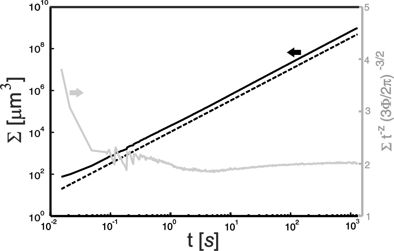
Figure 5: Time evolution of the maximum droplet size (same parameters as in Fig. 3). The black solid line represents the values inferred from our simulations. The black dashed line has a slope of $3/2$ on the double logarithmic axes, proving that $\Sigma\sim t^{3/2}$, and it represents the function $y=(3\Phi t/2\pi)^{z}$. The gray solid line is a reduced plot, obtained by dividing $\Sigma$ by the RHS (right hand side) of Eq. (8).

IV.1 Setup of simulations and growth of the largest droplets

All simulations start from an initial condition where $N_{0}=1.5\times 10^{5}$ droplets form an equispaced necklace at the distance $\lambda^{*}$ from each other; the length of the fiber $L_{f}$ is adapted accordingly. The initial conditions differ by a slight polydispersity of the droplet radii, which are chosen as $r_{0,i}=R_{\text{min}}(1+0.01\,I_{\text{rand},i})$ where $1\leq i\leq N_{0}$, and $I_{\text{rand},i}$ are random numbers in the interval $0\leq I_{\text{rand},i}\leq 1$ . We select the characteristic size of the distribution, $\Sigma(t)$, to be the maximum droplet size at time $t$. As predicted by Eq. (8), it scales as $\Sigma\sim\left(\frac{3\Phi}{2\pi}t\right)^{z}$ , with $z=3/2$ (Fig. 5). The asymptotic value of 2 in the reduced plot indicates that most likely the largest droplet in the system has recently undergone a collision.

IV.2 Scaling of the droplet number and the porosity

We check the consistency of the exponents for $p^{*}(t)$ and $N(t)$ by inspecting Eq. (19) and Eq. (13b), respectively.

In order to improve the statistics, we run five simulations for each case, with different but equivalent initial conditions. To this aim, we take different seeds in the random number generator used to create the initial distribution of the radii. The curves $p^{*}(t)$ and $N(t)$ for different random numbers seeds all lie on top of each other, and they have the same scattering of the data (see Figs. 6 and 7). The five runs produced data at time instants which were not perfectly in-phase, due to the event-driven nature of the model. Therefore, we use the curves $p^{*}(t)$ and $N(t)$, produced by overlapping the individual curves of the five runs, to extract the exponents $k$ and $z^{\prime}$ respectively.

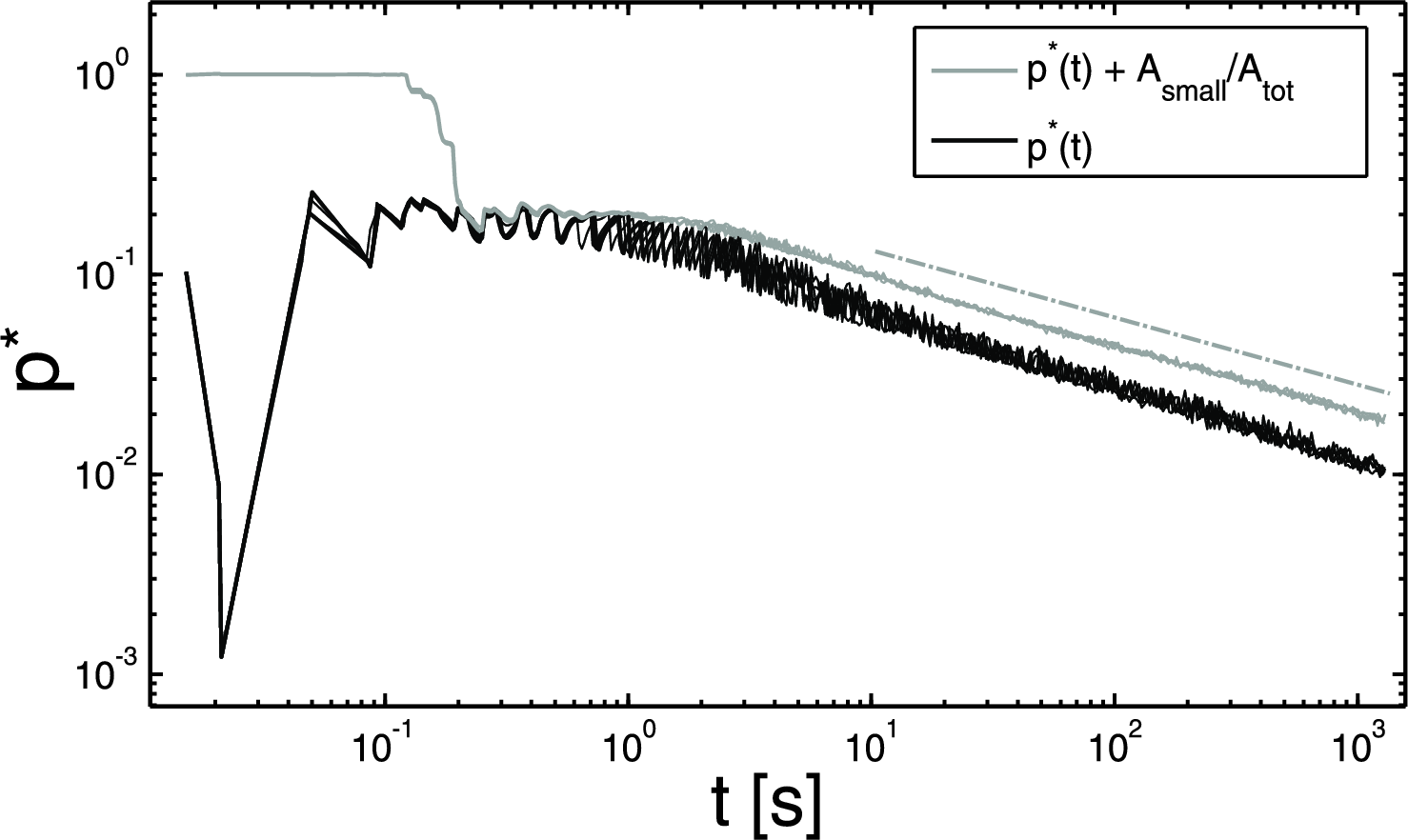
Figure 6: Time evolution of the effective porosity (same parameters as in Fig. 3). The lower lines (black) represent the total effective porosity, as defined in Eq. (14), for five simulations with different but equivalent initial conditions; the upper lines (gray, solid) represent the partial effective porosity $\bar{p}^{*}=1-A^{*}/A_{\text{tot}}$, where $A^{*}$ is the sum of the areas (lengths) covered by the droplets of size $s>\lambda^{*3}$. The gray dashed line represent the line used to fit the porosity $\bar{p}^{*}$ and it has a slope $-k=-0.332\pm 0.003$, on the log-log axes. From this we estimate $\tau=1.112\pm 0.002$.

In Fig. 6 we show the time evolution of the modified porosity $p^{*}(t)$, for five equivalent initial conditions. The following parameters were used: $\varepsilon=2\%$, $R_{f}=R_{\text{min}}=1\,\mu$m, $\Phi=1000\,\mu$m${}^{2}/$s. The lower lines (black) represent the total effective porosity, as defined in Eq. (14). The upper lines (gray, solid) represent the partial effective porosity $\bar{p}^{*}=1-A^{*}/A_{\text{tot}}$, where $A^{*}$ is the sum of the areas (lengths) covered by the droplets of middle and large size. Specifically, we keep into account only the droplets of size $s_{c}>\lambda^{*3}$ and we use these curves to find the exponent $k$. As pointed out at the end of Sect. III.4, this choice does not affect the resulting exponent, but it reduces the fluctuations related to the microscopic details of the nucleation of new droplets. The gray dashed line shows the best fit of the slope $-k$ calculated from fitting the modified porosities $\bar{p}^{*}$ of the five simulations. For the considered parameters, we obtain $k=0.332\pm 0.003$.

In Fig. 7 we show the time evolution of the number of droplets, for the same data of Fig. 6. The dark gray thin lines (blue online) represent the total number of droplets $N(t)$. The black lines represent the number of the large droplets: $s/\Sigma(t)>0.75^{3}$; by fitting them we estimate a decaying exponent of $0.503\pm 0.026\simeq 1/2$, in agreement with the theoretical prediction for a monodisperse droplet populations (see Eq. (13b), for $\tau\leq 1$). The lit-gray thin lines (green online) depict the number of the small droplets, with $s/\Sigma(t)<x_{N0}(t)$ and $x_{N0}(t)=\lambda^{*3}/\Sigma(t)$. They suffer from large oscillations, reflecting the repopulation of large areas that are episodically released by the merging of large droplets. The gray thick lines (red online) show the number of droplets of middle and large size, with $s>\lambda^{*3}$, as defined above. We use these lines to find the exponent characterizing the decay of the number of droplets in time $z^{\prime}=0.329\pm 0.002$. From Eq. (13b) and Eq. (19), we expect $k=z^{\prime}$, which is verified within the estimated error; the relative error on the average value is $\sim 0.4\%$. From Eq. (19), we derive the polydispersity exponent of the droplet size distribution $\tau=1.112\pm 0.002$, which is within the physically acceptable range $1<\tau<\theta$.

IV.3 Droplet number density

We calculate $n(s,t)$ from our numerical data by dividing the range of the sizes $s$ into $N_{\text{bins}}$ bins of width $\Delta s_{j}$, centered around $s_{j}$, where $j=1,..,N_{\text{bins}}$. At each time instant, we then calculate the droplet number density $n(s_{j},t)$ by counting how many droplets lie in the respective bins, $(s_{j}-\Delta s_{j}/2)<s^{*}<(s_{j}+\Delta s_{j}/2)$, and dividing the respective numbers by $(L_{f}\Delta s_{j})$, where $L_{f}$ is the total length of the fiber. We then take the average of the resulting droplet size distributions over 10 time instants and over five simulations with different but equivalent initial conditions, each one with initial droplet number $N_{0}=1.5\times 10^{5}$. The considered time instants are in the self-similar regime ($t>1000$ s) and they have been chosen in such a way to have 100 points per time decade. In particular they belong to the time range $1000$ s $<t<2000$ s.

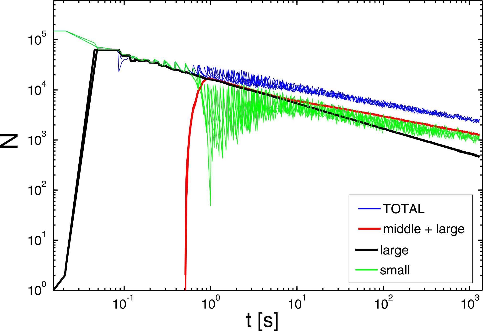
Figure 7: (Color online) Time evolution of the number of droplets per unit length (same parameters as in Fig. 3). The dark gray thin lines (blue online, uppermost right, denoted as ”TOTAL” in the legend) represent the total number of droplets $N(t)$, for 5 simulations with different but equivalent initial conditions. The lit-gray thin lines (green online) represent the number of the small droplets, with $s\leq\lambda^{*3}$ and its large oscillations. The mid-gray thick lines (red online) represent the number of large and middle size droplets, with $s>\lambda^{*3}$; upon fitting, we derive a decaying exponent $z^{\prime}=0.329\pm 0.002$. The black lines represent the number of the large droplets, with $s/\Sigma(t)>0.75^{3}$; their decaying exponent is $0.503\pm 0.026\simeq 1/2$, in agreement with the theoretical prediction for a monodisperse droplet population.

The resulting distribution $n(s,t)$ is shown in Fig. 3 (black solid line). The gray solid line and the gray dashed line represent our numerical estimate of the cutoffs for the large droplets $\hat{f}(s/\Sigma(t))$ and for the small droplets $\hat{g}(s/s_{0})$, respectively. They are obtained from Eq. (9), with the specific choice for the cutoff asymptotes $\hat{f}(s/\Sigma(t))=\hat{f}_{0}=$const for $s/\Sigma(t)\leq 1\%$, and $\hat{g}(s/s_{0})=1$ for $s\geq\lambda^{*}$.

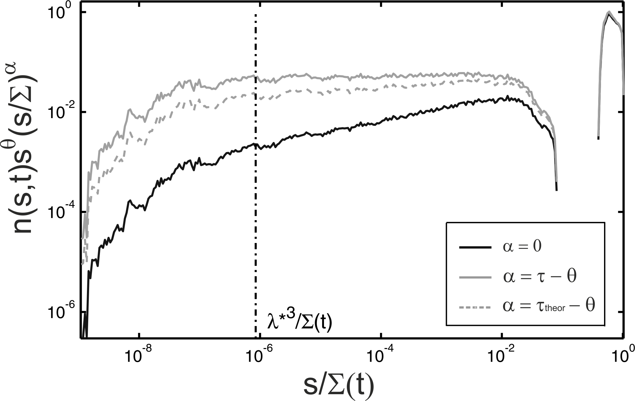
Figure 8: Droplet number density $n(s,t)$ (same parameters as in Fig. 3). The black line represents $n(s,t)s^{\theta}$. The gray solid line represents the same quantity rescaled: $n(s,t)s^{\theta}(s/\Sigma)^{\tau-\theta}$, with $\tau=1.112$, from the porosity fit: such an estimate seems to be consistent, since the plotted curve is horizontal, in the self-similar range (middle size droplets). The gray dashed line represents the same rescaled quantity with $\tau_{\text{theor}}=7/6$ Blackman and Brochard (2000): such a value is not consistent, since the plotted curve is not horizontal, in the range of self-similar sizes. The present graphs are derived by averaging the droplet size distributions over 10 time instants and over five simulations with different but equivalent initial conditions. The considered instants are in the self-similar regime ($t>1000s$) and they are chosen in such a way to have 100 points per time decade.

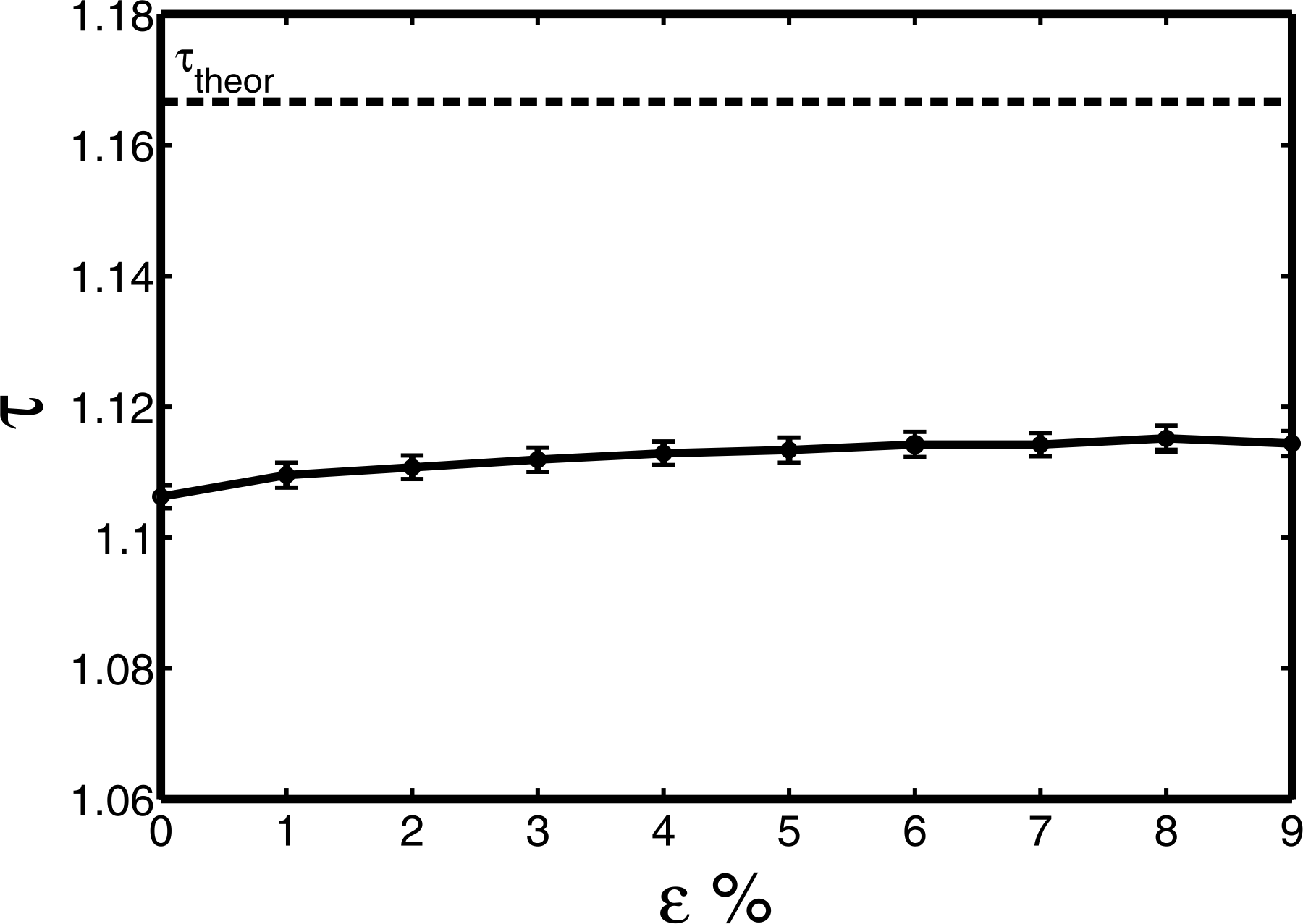
(a)              (b)  

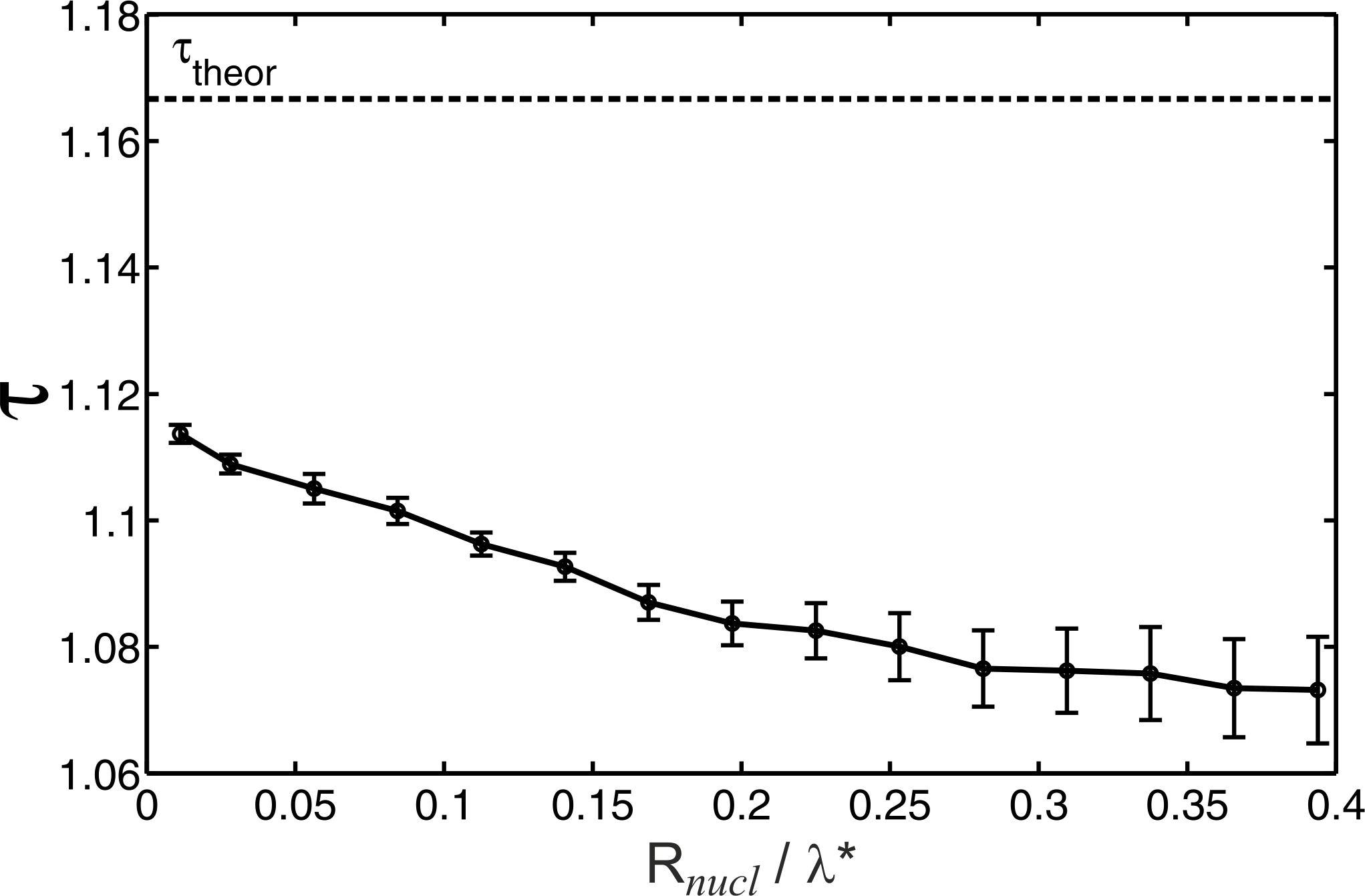
Figure 9: The exponent $\tau$ as a function of (a) the interaction range, $\varepsilon$, and (b) the ratio among the radius of the nucleated droplets $R_{\text{nucl}}$ and the characteristic length of the perturbation originating the droplets chain $\lambda^{*}$. The solid lines represent the values of $\tau$ inferred from the fit of the effective porosity. The dashed line is the theoretical value predicted by the classical theory for breath figures Blackman and Brochard (2000) $\tau_{\text{theor}}=7/6$. The parameters in (a) are $R_{f}=R_{\text{min}}=1\,\mu$m, $\Phi=1000\,\mu$m${}^{2}/$s, and $N_{0}=1.5\times 10^{5}$, while for (b) we used $\varepsilon=0\%$, $\Phi=1000\,\mu$m${}^{2}/$s, and $N_{0}=1.5\times 10^{5}$.

In Fig. 8, we show the droplet number density rescaled in such a way to make it dimensionless. The black solid line represents the quantity $n(s,t)s^{\theta}$. With the gray solid line we introduce a further rescaling $n(s,t)s^{\theta}(s/\Sigma(t))^{\tau-\theta}$, in order to verify the estimate of $\tau=1.112$ from the fit of the effective porosity. The gray dashed line depicts the same quantity, rescaled with the theoretical prediction $\tau_{\text{theor}}=7/6$ Blackman and Brochard (2000). The gray solid line is horizontal, in the range of sizes corresponding to the self-similar regime, while the gray dashed line has a slight positive slope. Consistently, our data support a polydispersity exponent considerably smaller than expected, but still matching the values obtained from the decay of the porosity Fig. 6 and the droplet number Fig. 7. The good agreement fully supports the classical scaling results relating the power-law dependencies of these quantities Beysens et al. (1991); Kolb (1989); Meakin (1992); Blackman and Brochard (2000).

IV.4 Parameter dependence of $\tau$

We repeated the procedure to calculate $\tau$ and to verify its accuracy, varying several parameters, in order to clarify its nature in terms of universality. In particular, we considered its dependence on the interaction range $\varepsilon$ between droplets, the nucleation radius $R_{\text{nucl}}$, the fiber radius $R_{f}$, the impinging water flux per unit length $\Phi$ and the monodispersity of the nucleated droplets chain. The variation of the latter, has been realized by randomly redistributing different percentages of the water volumes $V_{\text{gap},i}$ accumulated on the $i^{th}$ gap, among the new nucleated droplets on the same gap. We found that changes in both the impinging flux $\Phi$ and the monodispersity of the nucleated droplets do not affect the exponent $\tau$, in line with expectations (see Sect. III). However, the exponent $\tau$ exhibits a clear dependence on the interaction range, as it grows with $\varepsilon$ (see Fig. 9(a), solid line). The ratio between the nucleation radius $R_{\text{nucl}}$ and the characteristic length of the perturbation $\lambda^{*}$ also has an influence on $\tau$. In particular, $\tau$ decreases with increasing $R_{\text{nucl}}/\lambda^{*}$ (see Fig. 9(b), solid line).

Remarkably, all measured values of $\tau$ are substantially different ($4$%–$8$%) from the theoretical prediction Blackman and Brochard (2000) demanding $\tau_{\text{theor}}=7/6$ (see Fig. 9, dashed lines). The difference is significant, since it exceeds 10 times the estimated error of the exponent.

The dependence of the $\tau$ exponent on the interaction range $\varepsilon$ can be explained as follows. Having larger interaction ranges $\varepsilon$ implies having a larger area released upon merging. One can see this by considering two merging droplets of radius $R_{1}$ and $R_{2}$, with interaction range $\varepsilon R_{1}$ and $\varepsilon R_{2}$ respectively. Just before the merging, they cover an area $A=2(R_{1}+R_{2})(1+\varepsilon)$. After the merging the covered area will be $A^{\prime}=2(1+\varepsilon)R^{\prime}$, where $R^{\prime}$ is the radius of the new generated droplet. Therefore, the released area, i.e. the generated gap, will be $\Delta g=2(1+\varepsilon)(R_{1}+R_{2}-R^{\prime})$. Larger generated gaps imply an enhancement in the nucleation process, because more space and more water volume are available for the new droplets. On the other hand larger gaps imply a delay in further merging processes. Such effects are particularly relevant when the merging droplets are large, i.e. when $(R_{1}+R_{2}-R^{\prime})$ is large. For increasing values of $\varepsilon$, one can then expect an increase in the number of small droplets and a decrease in the number of large droplets. Since $-\tau$ represents the slope of the size distribution of the droplets $n(s,t)$ (see Fig. 3), this will result into higher values of $\tau$ (see Fig. 9(a), solid line).

The dependence of $\tau$ on the ratio $R_{\text{nucl}}/\lambda^{*}$ can be explained through the following qualitative argument. We consider the case where the nucleation radius $R_{\text{nucl}}$ changes, but the characteristic length of the perturbation $\lambda^{*}$ remains constant, as well as all the other parameters. Given a certain newly generated gap of size $l_{i}^{0}$, the number of possible nucleation sites $N_{i}$ inside such a gap does not change with $R_{\text{nucl}}$, but only with $\lambda^{*}$, since $N_{i}=\lfloor l_{i}^{0}/\lambda^{*}\rfloor$. The time interval $\Delta t$ during which $N_{i}$ droplets can nucleate is the time required to reduce the gap size from $l_{i}^{0}$ to $N_{i}\lambda^{*}$. After that time, only $N_{i}-1$ droplets will have the space to nucleate inside the gap. However, the water volume required to have a nucleating chain of $N_{i}$ droplet is larger for larger $R_{\text{nucl}}$ and criterion (7) may not be matched during the time interval $\Delta t$. Therefore, for larger $R_{\text{nucl}}$, a smaller number of new droplets will appear, before the gap closes. Overall, a lower number of small droplets will be present in the system, hence a larger number of big droplets, due to mass conservation. Therefore, for increasing $R_{\text{nucl}}/\lambda^{*}$, the exponent $\tau$ will decrease (see Fig. 9(b), solid line).

IV.5 Origins of the discrepancy with $\tau_{\text{theor}}=7/6$

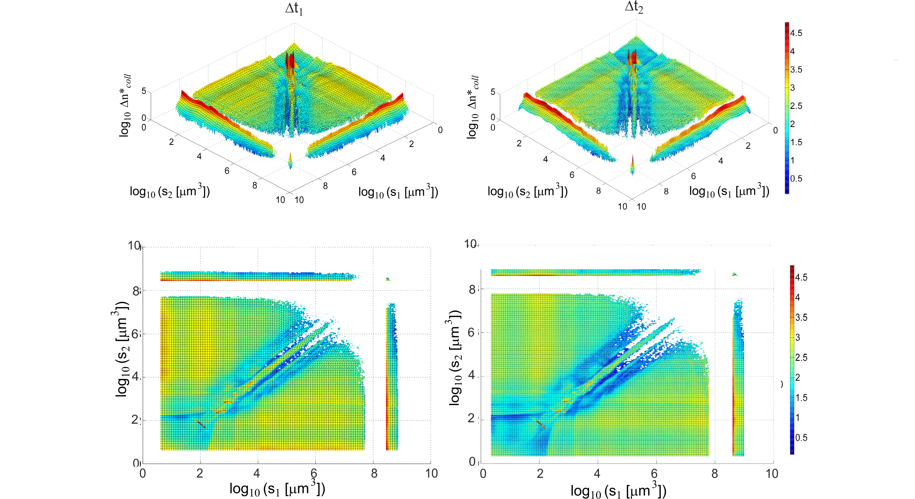
Figure 10: Reduced number density of collisions per unit length $\Delta n^{*}_{\text{coll}}$, during two different time intervals $\Delta t_{1}=t_{1}-t_{0}$ (left) and $\Delta t_{2}=t_{2}-t_{1}$ (right), with $t_{0}=480.5$ s, $t_{1}=1035.3$ s, $t_{2}=1308.9$ s (same parameters as in Fig. 3). To a good approximation, the plotted quantities are independent of time. However, they show a non-trivial dependence on $s_{1}$ and $s_{2}$.

The theoretical prediction Blackman and Brochard (2000), $\tau_{\text{theor}}=7/6$, is based on the assumption that the collision rate between two droplets of size $s_{1}$ and $s_{2}$ can be factorized as described in Eq. (20). When one adopts the hypothesis that $\tau$ takes a universal value, this approximation can be conveniently chosen to calculate the values of $\tau$. When $\tau$ depends on the microscopic details of the dynamics, as observed in Fig. 9, such an assumption must be tested for the data at hand.

To determine the collision rate for our numerical data, we count the number of collisions per unit length per unit size in two different time intervals $\Delta t_{1}=t_{1}-t_{0}$ and $\Delta t_{2}=t_{2}-t_{1}$, both in the self-similar regime of the droplets. In order to have a better statistics, we average the sets of results from five simulations with equivalent initial conditions. These numerical data are then compared to the integral of Eq. (20) between $t$ and $t+\Delta t$. Upon substitution of the expressions for $n(s,t)$ and $N(t)$ given by Eqs. (9) and III.3 respectively, we find

$$\Delta n_{\text{coll}}(s1,s2;t,\Delta t) \sim \tilde{H}\;(s_{1}s_{2})^{(1-3\tau)/D}\;(s_{1}^{1/D}+s_{2}^{1/D})\left[(t+\Delta t)^{3\tau/2-1}-t^{3\tau/2-1}\right]$$ (21a)

$$\text{where }\tilde{H} = \hat{f}\left(\frac{s_{1}}{\Sigma(t)}\right)\;\hat{g}\left(\frac{s_{1}}{s_{0}}\right)\;\hat{f}\left(\frac{s_{2}}{\Sigma(t)}\right)\;\hat{g}\left(\frac{s_{2}}{s_{0}}\right)\,.$$ (21b)

Consequently, Eq. (20) implies that

$$\Delta n_{\text{coll}}^{*}=\frac{\Delta n_{\text{coll}}(s1,s2;t,\Delta t)}{\tilde{H}\;(s_{1}s_{2})^{(1-3\tau)/D}\;(s_{1}^{1/D}+s_{2}^{1/D})\left[(t+\Delta t)^{\frac{3\tau}{2}-1}-t^{\frac{3\tau}{2}-1}\right]}=\text{const}\,.$$ (22)

Hence, the reduced number density of collisions per unit length of substrate $\Delta n_{\text{coll}}^{*}$ should be independent of the time $t$ and the sizes of the colliding droplets $s_{1}$, $s_{2}$. In Fig. 10 we plot the reduced number density of collisions per unit length of substrate $\Delta n_{\text{coll}}^{*}$ during the intervals $\Delta t_{1}$, $\Delta t_{2}$. In particular, we use the same set of data of Fig. 3 and we take $t_{0}=480.5$ s, $t_{1}=1035.3$ s , $t_{2}=1308.9$ s. We find that $\Delta n_{\text{coll}}^{*}$ is indeed invariant in time, to a good approximation (see Fig. 11). However, in variance with the assumed expression for the collision rate, Eq. (20), it depends on $s_{1}$ and $s_{2}$. In Fig. 11(a) we show a cross section of Fig. 10 along the main diagonal $s_{1}=s_{2}=s$, both for the first time interval $\Delta t_{1}$ (dashed line) and the second time interval $\Delta t_{2}$ (solid line). In other words, we display the reduced number of collisions between droplets of the same size. The data present pronounced, very sharp peaks, which do not move in time. The first peak, at $s^{*}_{0}$, corresponds to an enhanced probability of having a collision between droplets originating at the same moment, upon nucleation in the same gap, when they reach the size $s^{*}_{0}=(\lambda^{*}/2)^{3}$ (see Fig. 4). The second highest peak corresponds to an enhanced probability of collision between droplets of size $s^{*}_{1}=\lambda^{*3}$. Following the mechanism described in Fig. 4, we infer that this peak accounts for collisions between droplets generated at the same moment in the same droplet chain, that have already collided once. An interpretation along the same lines can be given for the peaks appearing at $s^{*}_{2}=(2\lambda^{*})^{3}$ and $s^{*}_{3}=(4\lambda^{*})^{3}$. With our simulation parameters, $s^{*}_{0}$ = 87 $\mu$m³ and $s^{*}_{1}$ = 700 $\mu$m³, $s^{*}_{2}$ = 5613 $\mu$m³ and $s^{*}_{3}$ = 44900 $\mu$m³. The intermediate peaks appearing between the main ones can be related to alternative merging mechanisms between droplets originated at the same moment in the same droplet chain. For example, the peak between $s^{*}_{0}$ and $s^{*}_{1}$, corresponds to a size $s^{*}_{1/2}\simeq(3/2\lambda^{*})^{3}$, suggesting a mechanism where every second droplet of the chain has already merged with its neighbor and the next merging takes place between droplets of alternated sizes $\lambda^{*}/2$ and $\lambda^{*}$. For colliding droplets larger than $s^{*}_{3}$, such mechanisms are not relevant anymore, thus suggesting the appearance of a self-similar area, where the system has lost memory of the microscopic details of the nucleation.

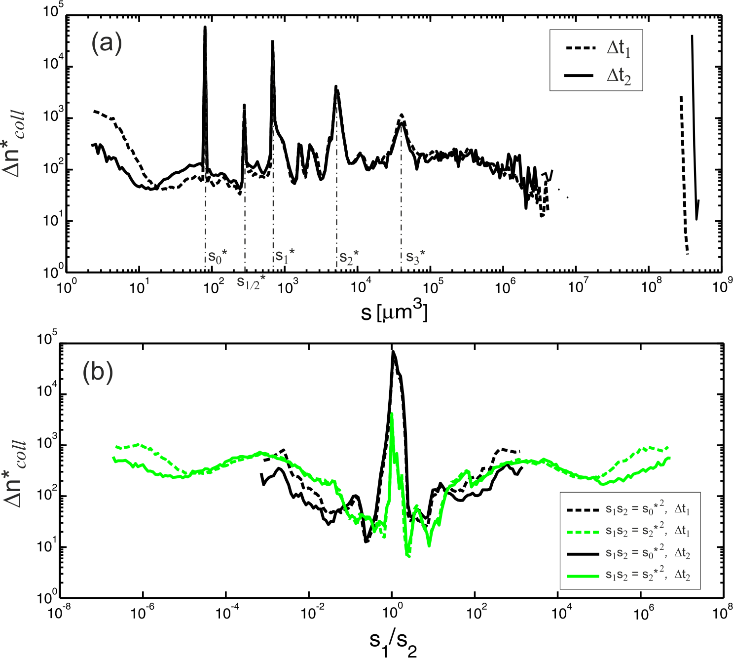
Figure 11: (Color online) Cross sections of the data displayed in Fig. 10 (a) along the main diagonal and (b) perpendicularly to it, during two different time intervals $\Delta t_{1}$ (dashed lines) and $\Delta t_{2}$ (solid lines). (a) Along the main diagonal, sharply defined maxima appear at sizes $s_{i}^{*}$ (with $i=0,\frac{1}{2},1,2,3$). (b) Perpendicularly to the main diagonal, along the lines $s_{1}s_{2}=(s_{0}^{*})^{2}$ (black lines) and $s_{1}s_{2}=(s_{2}^{*})^{2}$ (lit-gray lines, green online), there are maxima at the diagonal $s_{1}/s_{2}=1$, dips to its left and right and a plateau for $|\log_{10}s_{1}/s_{2}|\gtrsim 3$.

Fig. 11(b) displays further cross sections of Fig. 10 during $\Delta t_{1}$ (dashed lines) and $\Delta t_{2}$(solid lines). These cross sections are perpendicular to the main diagonal, and they show the peaks appearing Fig. 11(a) at $s^{*}_{0}$ (black lines) and $s^{*}_{2}$ (lit-gray lines, green online). The data display a recurring structure, with a peak corresponding to the main diagonal, and a dip just next to it. Such a structure is present along the whole main diagonal, as soon as the droplets are large enough to allow for secondary nucleation in the emerging gaps. The peak corresponds to the collisions between droplets of the same size. The dip surrounding the peak can be explained through the concept of self-similarity itself. The global droplet size distribution $n(s,t)$ can be regarded as a superposition of bimodal droplet size distributions, with the same shape displayed in Fig. 3, but different values of $\Sigma$. If we consider a generic portion of the area occupied by the droplets, where the largest size is $\Sigma^{*}$, the rescaled droplet size distribution of such an area will present several droplets of similar size $\Sigma^{*}$ (see the bump in Fig. 8), from which, the peaks centered on the main diagonal in Fig. 10 originate. Such local droplet size distribution will also present a gap similar to the one of Fig. 3, from which the dips of Fig. 11(b) originate.

We conclude that the factorization of the collision rate $\dot{n}_{\text{coll}}$ Eq. (20), based on the assumption of the distribution of the droplets sizes $s_{1}$ being uncorrelated to the distribution of the sizes of the neighbors $s_{2}$, does not hold for our data.

V Conclusions

So far, only few numerical Derrida et al. (1990, 1991); Meakin (1991) and experimental works Steyer et al. (1990) have specifically addressed breath figures on a one-dimensional substrate. Performing repeatable and controllable experiments for droplets on a fiber presents technical difficulties, such as keeping the temperature of a thin fiber constant. Quasi-one-dimensional settings have been realized by means of scratches on a plate Steyer et al. (1990), which allowed for a better control of the temperature of the substrate.

From the classical theory of breath figures it is known that the size distribution of droplets on a substrate becomes self-similar after some time that the system evolves; therefore it can be described by means of scaling laws, at least in the intermediate range of droplets sizes (the polydisperse range). In particular, two scaling exponents appear: $\theta$ and $\tau$. The value of $\theta$ can be inferred from dimensional analysis, while the value of the polydispersity exponent $\tau$ is non-trivial. The present work investigated the dependence of this exponent on the microscopic details of the system, in order to verify the recent finding Blaschke et al. (2012) that $\tau$ might not be universal, as commonly assumed. We developed an event-driven model for three-dimensional droplets on a one-dimensional substrate (fiber). We included the following details: the growth of the droplets by mass deposition from an impinging flow of supersaturated vapor, the precursor film between adjacent droplets, the nucleation process by surface tension driven instability and the merging of adjacent droplets. We calculated $\tau$, as well as the exponents characterizing the decay in time of the porosity and the number of droplets. The relations among these three exponents derived in the classical scaling analysis Beysens et al. (1991); Kolb (1989); Meakin (1992); Blackman and Brochard (2000), hold also for our model. As expected, we found that the exponent $\tau$ does not depend on the impinging mass flow and on the monodispersity level of the nucleation process. However, it does depend on the interaction range $\varepsilon$ of the droplets and on the ratio between the nucleation radius $R_{\text{nucl}}$ and the spacing $\lambda^{*}$ between the nucleating droplets. In particular, $\tau$ grows with increasing interaction ranges $\varepsilon$ and decreasing ratios $R_{\text{nucl}}/\lambda^{*}$. Our results contradicts the expectation that the exponent $\tau$ should be universal. Additionally, the values of $\tau$ that we inferred from our simulations differ by 10 standard deviations from the theoretical prediction $\tau_{\text{theor}}=7/6$ Blackman and Brochard (2000). Such a prediction was based on the assumption that the probabilities of having two neighboring droplets of prescribed sizes are uncorrelated. We analyzed the distribution of the collisions respect to the sizes of the colliding droplets and we showed that this assumption is inaccurate when one keeps into account the microscopic details of the system.

Our observations pose new questions on the non-universal nature of the polydispersity exponent $\tau$, such as the specific mechanisms underlying its parametric dependence as well as its quantitative values. These questions have been raised here for a setting where the flux impinging on the droplets is proportional to the wetted length on the fiber, i.e. a situation where the droplet growth is limited by the diffusive mass transport to the fiber. Alternatively, one could also consider a setting where the droplets grow in proportion to their total surface area. The classical expectation was that this change of the microscopic details of the droplet growth should not affect the value of $\tau$. In order to test this expectation and to address the emerging questions, further numerical simulations should be developed, as well as a new theoretical framework accounting for the non-universal nature of $\tau$.