A Discrete Tchebichef Transform Approximation for Image and Video Coding

Abstract

In this paper, we introduce a low-complexity approximation for the discrete Tchebichef transform (DTT). The proposed forward and inverse transforms are multiplication-free and require a reduced number of additions and bit-shifting operations. Numerical compression simulations demonstrate the efficiency of the proposed transform for image and video coding. Furthermore, Xilinx Virtex-6 FPGA based hardware realization shows 44.9% reduction in dynamic power consumption and 64.7% lower area when compared to the literature.

1 Introduction

The discrete Tchebichef transform (DTT) is a useful tool for signal coding and data decorrelation [1]. In recent years, signal processing literature has employed the DTT in several image processing problems, such as artifact measurement [2], blind integrity verification [3], and image compression [4, 5, 6, 7]. In particular, the 8-point DTT has been considered in blind forensics for integrity check of medical images [3]. For image compression, the 8-point DTT is also capable of outperforming the 8-point discrete cosine transform (DCT) in terms of average bit-length in bitstream codification [4]. Moreover, in [7] an 8-point DTT-based encoder capable of improved image quality and reduced encoding/decoding time was proposed; being a competitor to state-of-the-art DCT-based methods. However, to the best of our knowledge, literature archives only one fast algorithm for the 8-point DTT, which requires a significant number of arithmetic operations [6]. Such high arithmetic complexity may be a hindrance for the adoption of the DTT in contemporary devices that demand low-complexity circuitry and low power consumption [8, 9, 10].

An alternative to the exact transform computation is the employment of approximate transforms. Such approach has been successfully applied to the exact DCT, resulting in several approximations [11, 12]. In general, an approximate transform consists of a low-complexity matrix with elements defined over a set of small integers, such as $\{0,\pm 1,\pm 2,\pm 3\}$. The resulting matrix possesses null multiplicative complexity, because the involved arithmetic operations can be implemented exclusively by means of a reduced number of additions and bit-shifts. Prominent examples of approximate transforms include: the signed DCT [13], the series of DCT approximations by Bouguezel-Ahmed-Swamy [14, 15, 16], the approximation by Lengwehasatit-Ortega [17], and the integer based approximations described in [11, 18, 12, 19].

In this work, we introduce a low-complexity DTT approximation that requires 54.5% less additions than the exact DTT fast algorithm. The proposed method is suitable for image and video coding, capable of processing data coded according to popular standards—such as JPEG [20], H.264 [21], and HEVC [22]—at a low computational cost. Moreover, the FPGA hardware realization of the proposed transform is also sought.

This paper unfolds as follows. Section 2 describes the DTT and introduces the approximate DTT with its associate fast algorithm. A computational complexity analysis is offered. In Section 3, we perform numerical experiments; applying of the proposed transform as a tool for image and video compression. In Section 4, we provide very large scale integration (VLSI) realizations of the exact DTT and proposed approximation. Conclusions and final remarks are in Section 5.

2 Discrete Tchebichef Transform Approximation

2.1 Exact Discrete Tchebichef Transform

The DTT is an orthogonal transformation derived from the discrete Tchebichef polynomials [23]. The entries of the $N$-point DTT matrix are furnished by [1]:

$$t_{k,n}= \sqrt{\frac{(2k+1)(N-k-1)!}{(N+k)!}}\cdot(1-N)_{k}\cdot{}_{3}F_{2}(-k,-n,1+k;1,1-N;1),\qquad k,n=0,1,\ldots,N-1,$$ (1)

where ${}_{3}F_{2}(a_{1},a_{2},a_{3};b_{1},b_{2};z)=\sum_{n=0}^{\infty}\frac{(a_{1})_{k}(a_{2})_{k}(a_{3})_{k}}{(b_{1})_{k}(b_{2})_{k}}\cdot\frac{z^{k}}{k!}$ is the hypergeometric function and ${(a)}_{k}=a(a+1)\cdots(a+k-1)$ is the ascending factorial. Therefore, the analysis and synthesis equations for the DTT are given by $\mathbf{X}=\mathbf{T}\cdot\mathbf{x}$ and $\mathbf{x}=\mathbf{T}^{-1}\cdot\mathbf{X}=\mathbf{T}^{\top}\cdot\mathbf{X}$, where $\mathbf{x}=\begin{bmatrix}x_{0}&x_{1}&\cdots&x_{N-1}\end{bmatrix}^{\top}$ is the input signal, $\mathbf{X}=\begin{bmatrix}X_{0}&X_{1}&\cdots&X_{N-1}\end{bmatrix}^{\top}$ is the transformed signal, and $\mathbf{T}$ is the $N$-point DTT matrix with elements $t_{k,n}$, $k,n=0,1,\ldots,N-1$,

In particular, the 8-point DTT matrix $\mathbf{T}$ can be described by the product of a diagonal matrix $\mathbf{F}$ and an integer-entry matrix $\mathbf{T}_{0}$ [6], resulting in: $\mathbf{T}=\mathbf{F}\cdot\mathbf{T}_{0}$, where

$$\mathbf{T}_{0}=\left[\hbox{}\,\vbox{\Let@\restore@math@cr\default@tag\halign{\hfil$\m@th\scriptstyle#$&&\thickspace\hfil$\m@th\scriptstyle#$\cr 1&1&1&1&1&1&1&\phantom{-}1\\ -7&-5&-3&-1&1&3&5&7\\ 7&1&-3&-5&-5&-3&1&7\\ -7&5&7&3&-3&-7&-5&7\\ 7&-13&-3&9&9&-3&-13&7\\ -7&23&-17&-15&15&17&-23&7\\ 1&-5&9&-5&-5&9&-5&1\\ -1&7&-21&35&-35&21&-7&1\crcr}}\,\right]$$

and $\mathbf{F}=\frac{1}{2}\cdot\operatorname{diag}\left(\frac{1}{\sqrt{2}},\frac{1}{\sqrt{42}},\frac{1}{\sqrt{42}},\frac{1}{\sqrt{66}},\frac{1}{\sqrt{154}},\frac{1}{\sqrt{546}},\frac{1}{\sqrt{66}},\frac{1}{\sqrt{858}}\right)$. A fast algorithm for the above integer matrix $\mathbf{T}_{0}=\mathbf{F}^{-1}\cdot\mathbf{T}$ was derived in [6] requiring 44 additions and 29 bit-shifting operations. Such arithmetic complexity is considered excessive, when compared to state-of-the-art discrete transform approximations which generally require less than 24 additions [12, 17, 13, 16].

2.2 DTT Approximation and Fast Algorithm

In [12], a class of DCT approximations was introduced based on the following relation: $\operatorname{round}(\alpha\cdot\mathbf{C})$, where $\operatorname{round}(\cdot)$ is the round function as defined in C and Matlab languages [12], $\alpha$ is a real parameter, and $\mathbf{C}$ is the exact DCT matrix. We aim at proposing a similar approach to obtain an 8-point DTT approximation. The scale-and-round approach is particularly effective when discrete trigonometric transforms are considered. This is because the entries of such transformation matrices have smaller dynamic ranges when compared to the DTT. In contrast, the DTT entries have values with a dynamic range roughly seven times larger than the DCT, for example. Thus the approximation error implied by the round function is less evenly distributed in non-trigonometric transform matrices, such as the DTT. To mitigate this effect, we propose a compading-like operation [24], consisting of a rescaling matrix $\mathbf{D}$ that normalizes the DTT matrix entries. Thus, according the formalism detailed in [12], we introduce a parametric family of approximate DTT matrices $\mathbf{T}(\alpha)$, which are given by:

$$\mathbf{T}(\alpha)=\operatorname{round}\left(\alpha\cdot\mathbf{T}\cdot\mathbf{D}_{0}\right),$$ (10)

where $\mathbf{D}_{0}=\operatorname{diag}(\sqrt{\frac{6}{7}},\frac{\sqrt{154}}{13},\frac{\sqrt{66}}{9},\frac{\sqrt{858}}{35},\frac{\sqrt{858}}{35},\frac{\sqrt{66}}{9},\frac{\sqrt{154}}{13},\sqrt{\frac{6}{7}})$.

We aim at identifying a particular optimal parameter $\alpha^{\ast}$ such that $\mathbf{T}^{\ast}=\mathbf{T}(\alpha^{\ast})$ results in a matrix satisfying the following constraints: (i) the entries of $\mathbf{T}^{\ast}$ must be defined over $\{-1,0,1\}$ and (ii) $\mathbf{T}^{\ast}$ must possess low arithmetic complexity. Constraint (i) implies the search space $(0,3/2)$. Although the above problem is not analytically tractable, its solution can be found by exhaustive search [12]. By taking the values of $\alpha$ over the considered interval in steps of $10^{-3}$, above conditions are satisfied for $0.931\leq\alpha^{\ast}\leq 0.957$. All values of $\alpha^{\ast}$ in this latter interval imply the same approximate matrix. Thus, the obtained low-complexity forward DTT approximation is given by:

$$\mathbf{T}^{\ast}= \left[\hbox{}\,\vbox{\Let@\restore@math@cr\default@tag\halign{\hfil$\m@th\scriptstyle#$&&\thickspace\hfil$\m@th\scriptstyle#$\cr 1&1&1&1&1&1&1&\phantom{-}1\\ -1&-1&0&0&0&0&1&1\\ 1&0&0&-1&-1&0&0&1\\ -1&1&1&0&0&-1&-1&1\\ 0&-1&0&1&1&0&-1&0\\ 0&1&-1&-1&1&1&-1&0\\ 0&-1&1&0&0&1&-1&0\\ 0&0&-1&1&-1&1&0&0\\ }}\,$$

and its inverse $\mathbf{T}^{\ast}$ is given by: $(\mathbf{T}^{\ast})^{-1}=\mathbf{T}_{1}\cdot\mathbf{D}_{1}$ where

$$\mathbf{T}_{1}= \left[\hbox{}\,\vbox{\Let@\restore@math@cr\default@tag\halign{\hfil$\m@th\scriptstyle#$&&\thickspace\hfil$\m@th\scriptstyle#$\cr 1&-3&3&-2&1&-1&-1&-1\\ 1&-2&-1&2&-1&1&-1&1\\ 1&-1&-1&1&-1&-2&3&-2\\ 1&-1&-1&1&1&-2&-1&3\\ 1&1&-1&-1&1&2&-1&-3\\ 1&1&-1&-1&-1&2&3&2\\ 1&2&-1&-2&-1&-1&-1&-1\\ 1&3&3&2&1&1&-1&1\\ }}\,\right]$$

and $\mathbf{D}_{1}=\operatorname{diag}\left(\frac{1}{8},\frac{1}{10},\frac{1}{8},\frac{1}{10},\frac{1}{4},\frac{1}{10},\frac{1}{8},\frac{1}{10}\right)$. Considering the total energy error [13, 18] between the exact and approximate matrices, we obtained $3.32$ and $4.86$ as the error values for the direct and inverse transformations, respectively. Such errors are considered very small [19].

Thus, employing the orthogonalization procedure described in [12], we obtain the following expression for the DTT approximation: $\hat{\mathbf{T}}=\mathbf{D}^{\ast}\cdot\mathbf{T}^{\ast}$, where $\mathbf{D}^{\ast}=\sqrt{\operatorname{ediag}\left(\mathbf{T}^{\ast}\cdot(\mathbf{T}^{\ast})^{\top}\right)}=\begin{bmatrix}d_{0}^{\ast}&d_{1}^{\ast}&d_{2}^{\ast}&d_{3}^{\ast}&d_{4}^{\ast}&d_{5}^{\ast}&d_{6}^{\ast}&d_{7}^{\ast}\end{bmatrix}^{\top}$ is a diagonal matrix and $\operatorname{ediag}(\cdot)$ returns a diagonal matrix with the diagonal elements of its matrix argument [12]. The inverse transformation is $(\hat{\mathbf{T}})^{-1}=(\mathbf{D}^{\ast}\cdot\mathbf{T}^{\ast})^{-1}=(\mathbf{T}^{\ast})^{-1}\cdot(\mathbf{D}^{\ast})^{-1}=\mathbf{T}_{1}\cdot\mathbf{D}_{1}\cdot(\mathbf{D}^{\ast})^{-1}$. Therefore, the analysis and synthesis equations for the proposed transform are given by $\hat{\mathbf{X}}=\hat{\mathbf{T}}\cdot\mathbf{x}$ and $\mathbf{x}=\mathbf{T}_{1}\cdot\mathbf{D}_{1}\cdot(\mathbf{D}^{\ast})^{-1}\cdot\hat{\mathbf{X}}$, where $\hat{\mathbf{X}}=\begin{bmatrix}\hat{X}_{0}&\hat{X}_{1}&\cdots&\hat{X}_{7}\end{bmatrix}^{\top}$ is the approximate transformed vector.

However, in several contexts, diagonal matrices—such as $\mathbf{D}_{1}$ and $\mathbf{D}^{\ast}$—represent only scaling factors and may not contribute to the computational cost of transformations. For instance, in JPEG-based image compression applications, diagonal matrices can be embedded into quantization block [11, 6, 12] and, when the explicit transform coefficients are needless, a scaled version of the transform-domain spectrum is sufficient [25]. Therefore, hereafter, we disregard the diagonal matrices and focus our analysis on the low-complexity matrices $\mathbf{T}^{\ast}$ and $\mathbf{T}_{1}$. A fast algorithm based on sparse matrix factorization [14, 11, 12] was derived for the proposed forward and inverse approximations. In Figure 1, the signal flow graph (SFG) for the direct transformation is depicted. The SFG for the inverse transformation can be obtained according to the methods described in [26]. Moreover, Table 1 summarizes the arithmetic complexity assessment for the proposed transformations. The fast algorithms for $\mathbf{T}^{\ast}$ and $\mathbf{T}_{1}$ demand 54.5% and 34.1% less additions than the DTT fast algorithm (ITT) proposed in [6], respectively.

Figure 1: Signal flow graph for $\mathbf{T}^{\ast}$. Input data $x_{n}$, $n=0,1,\ldots,7$, relates to the output $\hat{X}_{k}$, $k=0,1,\ldots,7$. Dashed arrows represent multiplications by $-1$. Scaling by $d_{k}^{\ast}$, $k=0,1,\ldots,7$, can be ignored and absorbed into the quantization step.

Table 1: Arithmetic complexity of the proposed 1-D transforms

Method	Mult.	Additions	Shifts	Total
Exact DTT [6]	0	44	29	73
Proposed $\mathbf{\hat{T}}^{\ast}$	0	20	0	20
Proposed $\mathbf{T}_{1}$	0	29	8	37

3 Experimental Results

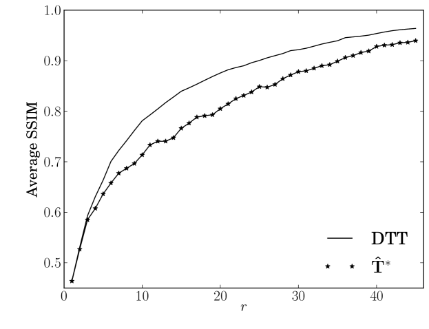
(a) SSIM

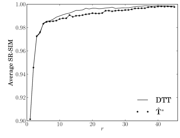
(b) SR-SIM

Figure 2: Quality metrics considering (a) SSIM and (b) SR-SIM for the exact DTT and the proposed approximation in terms of $r$.

3.1 Image Compression

In order to assess the proposed transform in image compression applications, we performed a JPEG-like simulation based on [11, 6, 12]. A set of 45 512$\times$512 8-bit grayscale images obtained from a standard public image bank [27] was considered. Each image was subdivided into 8$\times$8 size blocks $\mathbf{A}_{i,j}$, $i,j=1,2,\ldots,64$. Each block is submitted to two-dimensional (2-D) versions of the discussed transformations according to: $\mathbf{B}_{i,j}=\mathbf{M}\cdot\mathbf{A}_{i,j}\cdot\mathbf{M}^{\top}$, where $\mathbf{B}_{i,j}$ is the transform-domain block and $\mathbf{M}\in\{\mathbf{T},\mathbf{T}^{\ast}\}$ The resulting 64 spectral coefficients of each block were ordered in the standard zigzag sequence. Subsequently, the $r$ initial coefficients in each block were retained and the remaining coefficients were discarded [12]. We adopted $1\leq r\leq 45$. Finally, each transform-domain subimage was submitted to inverse 2-D transformations and the full image was reconstructed. Image quality measures were employed to assess the degradation between original and reconstructed images. The considered measures were the structural similarity index (SSIM) [28] and the spectral residual base similarity (SR-SIM) [29]. These measures have the distinction of being consistent with subjective ratings [30, 29]. The peak signal-to-noise ratio (PSNR) was not considered as a figure of merit because of its limited capability of capturing the human perception of image fidelity and quality [31]. For each value of $r$, we considered average measures across all considered images. Such methodology is less prone to variance effects and fortuitous data. Figure 2 shows the resulting SSIM and SR-SIM measurements. The proposed transform performed very closely to the exact DTT. For qualitative purposes, Figure 3 shows compressed images according to the DTT and the proposed approximation for $r=6$; images are visually indistinguishable.

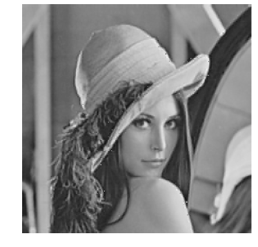
(a) DTT, $r=6$

(b) $\mathbf{\hat{T}}^{\ast},r=6$

Figure 3: Compressed ‘Lena’ image for $r=6$ by means of the (a)  DTT and (b) the proposed approximation.

3.2 Video Compression

With the objective of assessing the proposed transform performance in video coding, we have embedded the proposed DTT approximation in the widely employed software library x264 [32] for encoding video streams into the H.264/AVC standard [21]. The 8-point transform employed in H.264/AVC is an integer approximation of the DCT that demands 32 additions and 14 bit-shifting operations [33]. In comparison, the proposed 8-point direct transform requires 38% less additions and no bit-shifting operations, while the proposed inverse transform requires 9% less additions and 43% less bit-shifting operations. We encoded eleven CIF videos with 300 frames at 25 frames per second from a public video database [34] with the standard and the modified libraries. In our simulation, we employed default settings and controlled the video quality by two different approaches: (i) target bitrate, varying from 100 to 500 kbps with a step of 50 kbps and (ii) quantization parameter (QP), varying from 5 to 50 with steps of 5 units. For video quality assessment, we submitted the luma component of the video frames to average SSIM evaluation relative to the Y component (luminance). Results are shown in Figure 4. Even in scenarios of high compression (low bitrate/high QP), the degradation related to the proposed approximation is in the order of 0.01 units of SSIM; therefore, very low. Figure 5 displays the first encoded frame of a standard video sequence at low target bitrate (200 kbps). The resulting compressed frames are visually indistinguishable.

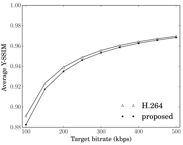
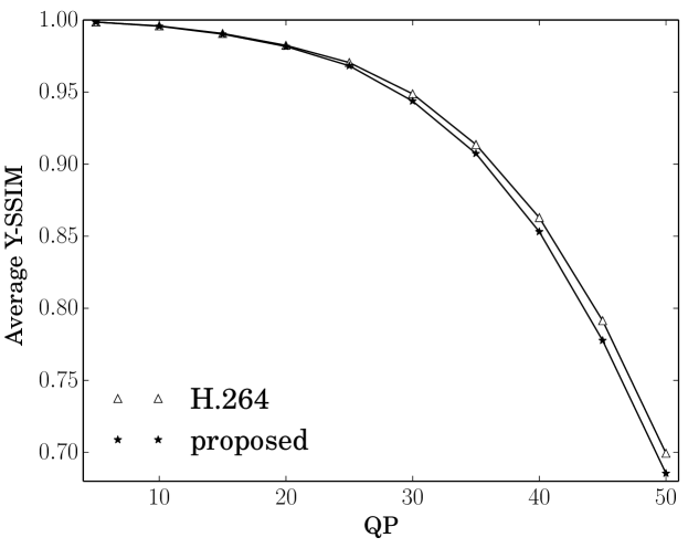
Figure 4: Video quality assessment in terms of (a) fixed target bitrate and (b) quantization parameter.

(a) H.264/AVC

(b) Modified H.264/AVC

Figure 5: First frame of the compressed sequence ‘Foreman’ according to (a) the original H.264/AVC and (b) modified H.264/AVC with the proposed approximation.

4 VLSI Architectures

To compare hardware resource consumption of the proposed approximate DTT against the exact DTT proposed in [6], the 1-D version of both algorithms were initially modeled and tested in Matlab Simulink and then were physically realized on a Xilinx Virtex-6 XC6VLX240T-1FFG1156 field programmable gate array (FPGA) device and validated using hardware-in-the-loop testing through the JTAG interface. Both approximations were verified using more than 10000 test vectors with complete agreement with theoretical values. Results are shown in Table 2. Metrics, including configurable logic blocks (CLB) and flip-flop (FF) count, critical path delay (CPD, in ns), and maximum operating frequency ($F_{\text{max}}$, in MHz) are provided. In addition, static ($Q_{p}$, in mW) and frequency normalized dynamic power ($D_{p}$, in mW/MHz) consumptions were estimated using the Xilinx XPower Analyzer. The final throughput of the 1-D DTT was $438.68\times 10^{6}$ 8-point transformations/second, with a pixel rate of $3.509\times 10^{9}$ pixels/second. The percentage reduction in the number of CLBs and FFs was 64.7% and 71%, respectively. The dynamic power consumption $D_{p}$ of the proposed architecture was 44.9% lower. The figures of merit area-time ($AT$) and area-time² ($AT^{2}$) had percentage reductions of 66.1% and 67.5% when compared with the exact DTT [6].

Table 2: Resource consumption on Xilinx XC6VLX240T-1FFG1156 device

Resource	Method
	Exact DTT [6]	Proposed
CLB ($A$)	408	144
FF	1370	396
CPD ($T$) (ns)	2.390	2.290
$F_{\text{max}}$ (MHz)​	418.41	438.68
$AT$	975.1	329.7
$AT^{2}$	2330.5	755.1
$D_{p}$ (mW/MHz)​	5.10	2.81
$Q_{p}$ (W)​	3.44	3.44

5 Conclusion

In this paper, a low-complexity approximation for the 8-point DTT was proposed. The arithmetic cost of the proposed approximation are significantly low, when compared with the exact DTT. At the same time, the proposed tool is very close to the DTT in terms of image coding for a wide range of compression rates. In video compression, the introduced approximation was adapted into the popular codec H.264 furnishing virtually identical results at a much less computational cost. Our goal with the codec experimentation is not to suggest the modification of an existing standard. Our objective is to demonstrate the capabilities of the proposed low-complexity transform in asymmetric codecs [35]. Such codecs are employed when a video is encoded once but decoded several times in low power devices [35, 36]. Additionally, the proposed transform can be considered in distributed video coding (DVC) [37, 36], where the computational complexity is concentrated in the decoder. A relevant context for DVC is in remote sensors and video systems that are constrained in terms of power, bandwidth, and computational capabilities [36]. The proposed approximation is a viable alternative to the DTT; possessing low-complexity and good performance according to meaningful image quality measures. Moreover, the associated hardware realization consumed roughly $1/3$ of the area required by the exact DTT; also the dynamic power consumption was decreased by 44.9%. Future work in this field may consider the evaluation of DTT approximations in quantization schemes [4, 5].

References

- [1] R. Mukundan, S. Ong, and P. A. Lee, “Image analysis by Tchebichef moments,” IEEE Transactions on Image Processing, vol. 10, no. 9, pp. 1357–1364, 2001.
- [2] L. Leida, Z. Hancheng, Y. Gaobo, and Q. Jiansheng, “Referenceless measure of blocking artifacts by Tchebichef kernel analysis,” IEEE Signal Processing Letters, vol. 21, pp. 122–125, Jan 2014.
- [3] H. Huang, G. Coatrieux, H. Shu, L. Luo, and C. Roux, “Blind integrity verification of medical images,” IEEE Transactions on Information Technology in Biomedicine, vol. 16, pp. 1122–1126, Nov 2012.
- [4] F. Ernawan, N. Abu, and N. Suryana, “TMT quantization table generation based on psychovisual threshold for image compression,” in 2013 International Conference of Information and Communication Technology (ICoICT), pp. 202–207, Mar 2013.
- [5] S. Prattipati, M. Swamy, and P. Meher, “A variable quantization technique for image compression using integer tchebichef transform,” in 2013 9th International Conference on Information, Communications and Signal Processing (ICICS), pp. 1–5, Dec 2013.
- [6] S. Prattipati, S. Ishwar, P. Meher, and M. Swamy, “A fast 88 integer Tchebichef transform and comparison with integer cosine transform for image compression,” in 2013 IEEE 56th International Midwest Symposium on Circuits and Systems (MWSCAS), pp. 1294–1297, 2013.
- [7] R. Senapati, U. Pati, and K. Mahapatra, “Reduced memory, low complexity embedded image compression algorithm using hierarchical listless discrete Tchebichef transform,” IET Image Processing, vol. 8, pp. 213–238, Apr 2014.
- [8] L. W. Chew, L.-M. Ang, and K. P. Seng, “Survey of image compression algorithms in wireless sensor networks,” in 2008 International Symposium on Information Technology (ITSim), vol. 4, pp. 1–9, Aug 2008.
- [9] F. Ernawan, E. Noersasongko, and N. Abu, “An efficient 22 Tchebichef moments for mobile image compression,” in 2011 International Symposium on Intelligent Signal Processing and Communications Systems (ISPACS), pp. 1–5, Dec 2011.
- [10] N. Kouadria, N. Doghmane, D. Messadeg, and S. Harize, “Low complexity DCT for image compression in wireless visual sensor networks,” Electronics Letters, vol. 49, pp. 1531–1532, Nov 2013.
- [11] R. J. Cintra and F. M. Bayer, “A DCT approximation for image compression,” IEEE Signal Processing Letters, vol. 18, pp. 579–582, Oct 2011.
- [12] R. J. Cintra, F. M. Bayer, and C. J. Tablada, “Low-complexity 8-point DCT approximations based on integer functions,” Signal Processing, vol. 99, pp. 201–214, 2014.
- [13] T. I. Haweel, “A new square wave transform based on the DCT,” Signal Processing, vol. 81, no. 11, pp. 2309–2319, 2001.
- [14] S. Bouguezel, M. Ahmad, and M. Swamy, “A multiplication-free transform for image compression,” in 2008 2nd International Conference on Signals, Circuits and Systems (SCS), pp. 1–4, Nov 2008.
- [15] S. Bouguezel, M. Ahmad, and M. Swamy, “A low-complexity parametric transform for image compression,” in 2011 IEEE International Symposium on Circuits and Systems (ISCAS), pp. 2145–2148, May 2011.
- [16] S. Bouguezel, M. Ahmad, and M. Swamy, “Binary discrete cosine and Hartley transforms,” IEEE Transactions on Circuits and Systems I: Regular Papers, vol. 60, pp. 989–1002, Apr 2013.
- [17] K. Lengwehasatit and A. Ortega, “Scalable variable complexity approximate forward DCT,” IEEE Transactions on Circuits and Systems for Video Technology, vol. 14, pp. 1236–1248, Nov 2004.
- [18] F. M. Bayer and R. J. Cintra, “DCT-like transform for image compression requires 14 additions only,” Electronics Letters, vol. 48, pp. 919–921, Jul 2012.
- [19] U. S. Potluri, A. Madanayake, R. J. Cintra, F. M. Bayer, S. Kulasekera, and A. Edirisuriya, “Improved 8-point approximate DCT for image and video compression requiring only 14 additions,” IEEE Transactions on Circuits and Systems I: Regular Papers, vol. 61, pp. 1727–1740, Jun 2014.
- [20] G. Wallace, “The JPEG still picture compression standard,” IEEE Transactions on Consumer Electronics, vol. 38, pp. xviii–xxxiv, Feb 1992.
- [21] I. Richardson, The H.264 Advanced Video Compression Standard. John Wiley and Sons, 2 ed., 2010.
- [22] G. Sullivan, J. Ohm, W.-J. Han, and T. Wiegand, “Overview of the high efficiency video coding (HEVC) standard,” IEEE Transactions on Circuits and Systems for Video Technology, vol. 22, no. 12, pp. 1649–1668, 2012.
- [23] H. Bateman, A. Erdélyi, W. Magnus, F. Oberhettinger, and F. Tricomi, Higher transcendental functions, vol. 2. McGraw-Hill, 1953.
- [24] R. Gray and D. Neuhoff, “Quantization,” IEEE Transactions on Information Theory, vol. 44, pp. 2325–2383, Oct 1998.
- [25] Y. Arai, T. Agui, and M. Nakajima, “A fast DCT-SQ scheme for images,” IEICE Transactions, vol. E71, pp. 1095–1097, Nov 1988.
- [26] R. Blahut, Fast Algorithms for Signal Processing. Cambridge University Press, 2010.
- [27] University of Southern California, Signal and Image Processing Institute, “The USC-SIPI image database.” http://sipi.usc.edu/database/, 2014.
- [28] Z. Wang, A. Bovik, H. Sheikh, and E. Simoncelli, “Image quality assessment: from error visibility to structural similarity,” IEEE Transactions on Image Processing, vol. 13, pp. 600–612, Apr 2004.
- [29] L. Zhang and H. Li, “SR-SIM: A fast and high performance IQA index based on spectral residual,” in 19th IEEE International Conference on Image Processing (ICIP), pp. 1473–1476, Sep 2012.
- [30] Z. Wang and A. Bovik, “Reduced- and no-reference image quality assessment,” IEEE Signal Processing Magazine, vol. 28, pp. 29–40, Nov 2011.
- [31] Z. Wang and A. Bovik, “Mean squared error: Love it or leave it? a new look at signal fidelity measures,” IEEE Signal Processing Magazine, vol. 26, pp. 98–117, Jan 2009.
- [32] x264 team, “x264.” http://www.videolan.org/developers/x264.html, 2014.
- [33] S. Gordon, D. Marpe, and T. Wiegand, “Simplified use of 88 transform – updated proposal and results.” Joint Video Team (JVT) of ISO/IEC MPEG and ITU-T VCEG, doc. JVT–K028, Munich, Germany, Mar 2004.
- [34] “Xiph.org Video Test Media.” https://media.xiph.org/video/derf/, 2014.
- [35] U. Mitra, Introduction to Multimedia Systems. Academic Press, 2004. 207 p.
- [36] K. R. Vijayanagar, J. Kim, Y. Lee, and J. bok Kim, “Low complexity distributed video coding,” Journal of Visual Communication and Image Representation, vol. 25, no. 2, pp. 361–372, 2014.
- [37] A. Wyner and J. Ziv, “The rate-distortion function for source coding with side information at the decoder,” IEEE Transactions on Information Theory, vol. 22, pp. 1–10, Jan 1976.