Morphologies introduced by bistability in barred-spiral galactic potentials

Abstract

We investigate the orbital dynamics of a barred-spiral model when the system is rotating slowly and corotation is located beyond the end of the spiral arms. In the characteristic of the central family of periodic orbits we find a “bistable region”. In the response model we observe a ring surrounding the bar and spiral arms starting tangential to the ring. This is a morphology resembling barred-spiral systems with inner rings. However, the dynamics associated with this structure in the case we study is different from that of a typical bar ending close to corotation. The ring of our model is round, or rather elongated perpendicular to the bar. It is associated with a folding (an “S” shaped feature) of the characteristic of the central family, which is typical in bistable bifurcations. Along the “S” part of the characteristic we have a change in the orientation of the periodic orbits from a x1-type to a x2-type morphology. The orbits populated in the response model change rather abruptly their orientation when reaching the lowest energy of the “S”. The spirals of the model follow a standard “precessing ellipses flow” and the orbits building them have energies beyond the “S” region. The bar is structured mainly by sticky orbits from regions around the stability islands of the central family. This leads to the appearance of X-features in the bars on the galactic plane. Such a bar morphology appears in the unsharp-masked images of some moderately inclined galaxies.

1 Introduction

In dynamical systems a “bistability situation” usually refers to cases where a system has two stable equilibrium states. In a bifurcation diagram the curve of steady state displays an “S” shape as a certain parameter of the system varies. The “S” is delimited by two saddle-node bifurcation points. Between them we have two stable and one unstable steady states (see e.g. Angeli et al, 2003; Lynch, 2007; Strogatz, 2014). The corresponding situation in Hamiltonian Galactic Dynamics is depicted in the characteristic of a family of periodic orbits as two successive tangent bifurcations (see e.g. Contopoulos, 2004) facing opposite directions. These two bifurcations share the same unstable branch. In other words the characteristic folds twice as the varying parameter, usually the Jacobi constant E_J ​, increases. Foldings of the characteristic have been encountered by Skokos et al. (2002a) and Skokos et al. (2002b), in 3D Ferrers bar potentials. However, the way they affect the face-on morphology of a model has not been examined in those papers. Nevertheless, it was clear that the foldings of the characteristics affect to a larger degree slowly rotating models. In this paper we present the implications of the presence of such a folding of the characteristic of the main family of periodic orbits for the dynamics of a slowly rotating barred-spiral potential.

Slowly rotating models of disc galaxies have been proposed in the past to describe the dynamics of normal (non-barred) spiral galaxies with open spiral arms. In these models (stellar and gaseous) the symmetric, strong spiral structure extends inside corotation (Contopoulos & Grosbøl, 1986, 1988; Patsis et al., 1991; Kranz et al, 2003; Martos et al, 2004; Junqueira et al, 2013).

Contrarily, in barred galaxy models corotation is usually placed close to the end of the bar (Contopoulos, 1980). Recently Font et al. (2014) presented a list with 32 barred galaxies in which they estimated the ratio of the corotation to the bar radius, $R_{c}/R_{b}$, to be between $0.94\pm 0.08<R_{c}/R_{b}<2.1\pm 0.5$. Model bars ending well inside corotation have been found in N-body simulations (Combes & Elmegreen, 1993) as well as in response models of barred potentials derived from near-infrared observations (Rautiainen et al., 2008). In all these studies, slowly rotating bars are associated with late-type barred-spiral galaxies. It is generally believed that bars in barred galaxies are supported by the x1 family of elliptical, stable, periodic orbits, which extends along the major axis of the bar (Contopoulos & Papayannopoulos, 1980), or, in the three-dimensional case, by the corresponding families of the x1-tree, i.e. by x1 together with 3D families bifurcated at the vertical resonances, (Skokos et al., 2002a). The bar is built by trapping quasi-periodic orbits along the orbits of these families. Deviations from this orbital behaviour have been proposed, pointing to bars in which other families than x1 play a significant and perhaps a leading role in the building of the bars. Such behaviours are favoured either in slowly rotating bar models in which the bars end well before corotation (Petrou & Papayannopoulos, 1986; Skokos et al., 2002b), or in bars with large major to minor axis ratios (Kaufmann & Patsis, 2005). Pasha & Polyachenko (1994) even claim, that in slowly rotating bars of the type described by Lynden-Bell (1979), there is a better matching of the outer-to-inner ring radial ratio, than in standard fast rotating bars. Finally, Patsis et al. (2010) have shown that bars of ansae-type can be supported mainly by chaotic orbits in a (fast rotating) model based on the potential of NGC 1300, estimated from near-infrared observations.

The implications of slow rotation for the orbital dynamics in a barred-spiral model, i.e. when the spiral component is explicitly included in the potential, have not been extensively studied. Recently Tsigaridi & Patsis (2013) have presented a barred-spiral model, rotating with a single pattern speed, characterized by a ratio $R_{c}/R_{b}$, about 2.9. This case, with $\varOmega_{p}=15$ km s^-1 kpc^-1 ​, has been considered as “general” since several dynamical mechanisms cooperated in forming the obtained barred-spiral response morphology. The action of two different dynamical mechanisms led to the formation of an inner barred-spiral structure surrounded by an oval-shaped disc and an outer set of spiral arms beyond corotation. However, if we decrease further the pattern speed, there are even more considerable changes in the orbital dynamics of the system. The pattern speed, $\varOmega_{p}$, is the most important parameter for the resulting response morphology of the model.

Besides the case presented in Tsigaridi & Patsis (2013), we have studied a series of models with even smaller $\varOmega_{p}$ down to 10 km s^-1 kpc^-1 ​. As the pattern speed decreases from $\varOmega_{p}=15$ km s^-1 kpc^-1 ​, we have a rather new orbital behaviour, which shapes a different barred-spiral response with distinct morphological features. For example, despite the fact that the bars in all studied models have comparable sizes, as $\varOmega_{p}$ decreases the orbital dynamics of the central family of periodic orbits changes from that of the typical case (Contopoulos & Grosbøl, 1989). In the present paper we present these changes, we describe the morphological features that are encountered in extremely slowly rotating models, and we discuss its relevance to some morphological features appearing in some images of barred-spiral galaxies.

Our general model is the same as in Tsigaridi & Patsis (2013). It is based on a modified version of a potential estimated from the near-infrared photometry of the late type barred-spiral galaxy NGC 3359 (Boonyasait, 2003; Patsis et al., 2009). We used it as a general barred-spiral potential with $\varOmega_{p}$ being a free parameter. It is worth noticing that Elmegreen & Elmegreen (1985), based on observation by Gottesman (1982), estimate the ratio of the semi-major axis of the bar to the length of the rising part of the rotation curve for NGC 3359 to be $R_{bar}/R_{rise}=0.75$. According to this work, the fact that the bar ends before the velocity curve turns over, is an indication for slow bar rotation. Despite the difficulties in estimating the inner parts of the rotation curves of barred galaxies, this property is in general associated with slowly rotating bars, like the bars of the models we study. In the series of our response models, since $R_{rise}\approx 4.6$ kpc (see figure 3 in Tsigaridi & Patsis, 2013) this ratio varies between 0.619 and 0.641. In the specific model of the present paper this ratio is about 0.62, close to the lowest value. This means that our potential is adequate for studying slowly rotating models in general.

The structure of the paper is the following: In Section 2 we briefly present again our potential (for more details see Tsigaridi & Patsis, 2013). The results of our study are described in Section 3 and refer to the building of the response features, which are the ring, the bar and the spirals. These results are discussed in Section 4 and in Section 5 we enumerate our conclusions.

2 Summary of model properties

The model has been extensively described in Tsigaridi & Patsis (2013). It is a two dimensional model of the general form

$$\Phi(r,\varphi)=\Phi_{0}(r)+\sum_{m=2,4,6}\Phi_{mc}(r)\,{\rm cos}\,(m\varphi)+\Phi_{ms}(r)\,{\rm sin}\,(m\varphi)$$ (1)

The components $\Phi_{0}$, $\Phi_{mc}$, and $\Phi_{ms}$ of the equation above are given as polynomials of the form $\sum_{n}\!\!a_{n}r^{n}$, $n=0\dots 8$. The radial variation of the perturbation force normalized over the radial axisymmetric one is given in figure 1 in Tsigaridi & Patsis (2013).

The equations of motion are derived from the Hamiltonian

$$H\equiv\frac{1}{2}\left(\dot{x}^{2}+\dot{y}^{2}\right)+\Phi(x,y)-\frac{1}{2}\Omega_{p}^{2}(x^{2}+y^{2})=E_{J},$$ (2)

where $(x,y)$ are the coordinates in a Cartesian frame of reference rotating with angular velocity $\Omega_{p}$. $\Phi(x,y)$ is the potential (1) in Cartesian coordinates with the bar aligned approximately with the y-axis, $E_{J}$ is the numerical value of the Jacobi constant, hereafter called the energy, and dots denote time derivatives.

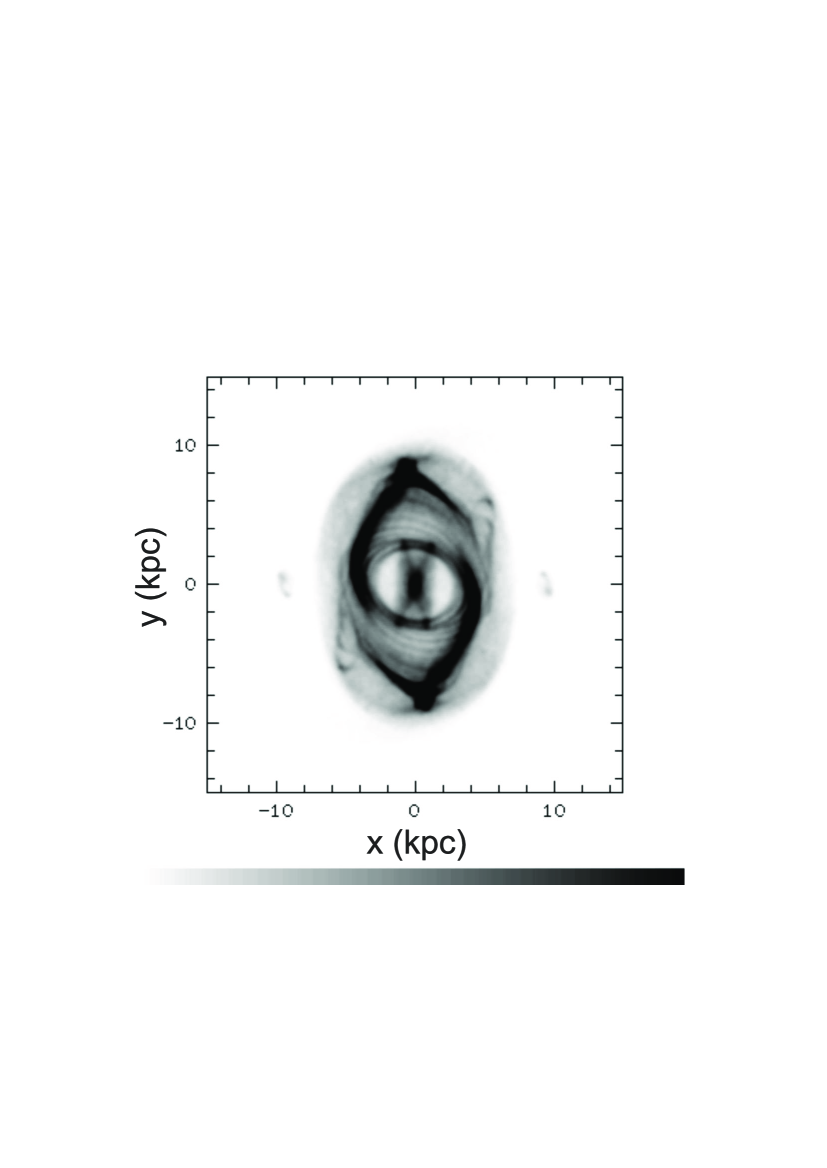
Figure 1: The stellar response model with $\varOmega_{p}=11.5$ km s^-1 kpc^-1 . The system has completed 10 pattern rotations, rotating counter-clockwise. The bar extends roughly along the y-axis. Corotation is at $R_{c}\approx$ 10 kpc

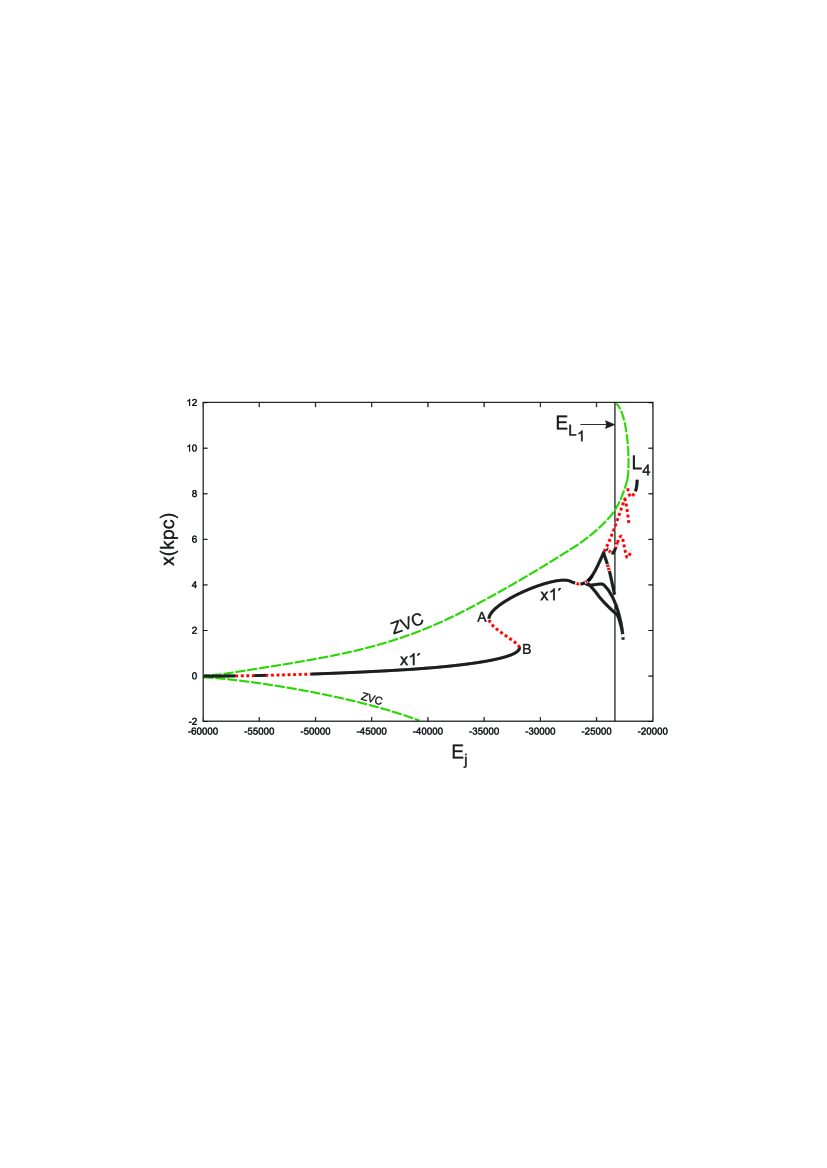
Figure 2: The characteristics of x1^′ and its bifurcations for $\varOmega_{p}=11.5$ km s^-1 kpc^-1 ​​. The dashed line, labelled “ZVC”, is the curve of zero velocity. Continuous black parts of the characteristic indicate stability, while dotted parts, red in the online version, instability. The $E_{L_{1}}$ line is indicated with an arrow in the upper right corner of the figure.

3 Slowly rotating models

By varying $\varOmega_{p}$ between $10<\varOmega_{p}<30$ km s^-1 kpc^-1 ​, we obtained always a kind of barred-spiral response. In this range of pattern speeds the corotation radius of the models, $R_{c}$, takes values between $12\gtrsim R_{c}\gtrsim 4.3$ kpc respectively. Nevertheless, while the pitch angle of the response spirals varied considerably in models with different pattern speeds (it was larger for lower pattern speeds), the radius of the response bar varied only between $2.85<R_{b}<2.95$ kpc. For $\varOmega_{p}>30$ km s^-1 kpc^-1 the size of the response bar was clearly decreasing. For example, for $\varOmega_{p}=35$ km s^-1 kpc^-1 we estimated it to be about 2.45 kpc.

The changes that are introduced in the dynamics of the system as $\varOmega_{p}$ decreases are reflected in changes observed in the (E_J ​​,$x)$ characteristic curve (for a definition see Contopoulos, 2004, section 2.4.3) of the central family. In typical cases of barred galaxy models, the $x_{0}$ initial condition of the central, x1, family is increasing with E_J between the inner Lindblad Resonance (ILR) and the 4:1 resonance (Contopoulos & Grosbøl, 1986, 1989). This is the case also for the present model for $\varOmega_{p}>16$ km s^-1 kpc^-1 $\!\!.$ However, for slower rotating models, i.e. for $\varOmega_{p}\lessapprox 15$ km s^-1 kpc^-1  ​​​, we observe a folding of the characteristic curve well before corotation in the (E_J ​​,$x)$ diagram. The $\Delta$E_J range over which we have the folding in a model increases with deceasing $\varOmega_{p}$. We call this feature, the “S”. As we will see, foldings of the characteristics introduce in the system new orbital dynamics accompanied by new morphological features. For this reason we call just in this work the central family of our model x1^′ in order to distinguish it from the standard x1 family, which has as members only elliptical periodic orbits elongated along the bar.

In the present paper we describe these changes in a typical case with $\varOmega_{p}=11.5$ km s^-1 kpc^-1 ​​ (chosen so that we have $R_{c}\approx$ 10 kpc). For this $\varOmega_{p}$ the morphological features associated with slow rotation dominate and this facilitates the description of the relevant dynamical mechanisms.

The stellar response model for the potential (1) with $\varOmega_{p}=11.5$ km s^-1 kpc^-1 is given in Fig. 1. The response bar length is $R_{b}\approx 2.85$ kpc. The system has completed 10 pattern rotations. Initially the particles have been distributed randomly within a disk of radius r_max=11 kpc with velocities securing circular motion in the axisymmetric part of the potential, $\Phi_{0}(r)$. At the beginning of the simulation the amplitudes $\Phi_{mc}$ and $\Phi_{ms}$ of the perturbing term grow linearly with time from 0 to their maximum value within two system periods (“time dependent phase”) and after that they remain constant. The time-dependency of the amplitudes in the beginning of the simulation secures a smooth response of the system, since the initial velocities are for circular motion in the axisymmetric term $\Phi_{0}(r)$.

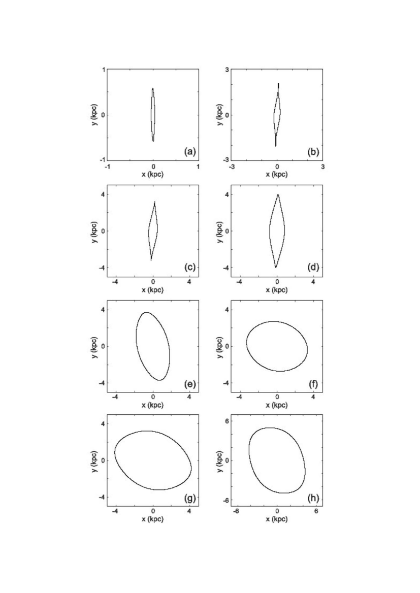
Figure 3: Periodic orbits along the characteristic of x1^′ for E_J = $-55000$ (a), $-45000$ (b), $-37000$ (c), $-33000$ (d),(e),(f) (the three x1^′ representatives at the “S” region), $-30000$ (g) and $-27000$ (h). Note the different scales of the axes.

The snapshot has been converted to an image using the ESO-Midas software. In the central part we observe a rectangular shaped bar. The contrast of the image has been chosen such as to allow us to clearly see that inside the rectangular shaped bar appears an “X” feature. The bar, with the embedded in it X-feature, ends on an oval (pseudo)ring structure. This ring has a certain width. It is almost round at its inner boundary, which is attached to the bar, while the ellipticity of the orbits that form it increases outwards and becomes maximum at its outer part, which coincides with the beginning of the spiral structure. At this point the ring is elongated in a direction roughly vertical to the bar (at an angle about $15^{\circ}$ with respect to the x-axis). The length of the semimajor axis of this ring is about 3.6 kpc. On the sides of the bar, inside the ring, the response surface density is very low. The double armed open spiral structure starts tangentially from the ring having a pitch angle $i_{p}\approx$ 35^∘in the outer parts (it is not logarithmic). The spiral arms have a sharp bifurcation at $r\approx 7.8$ kpc.

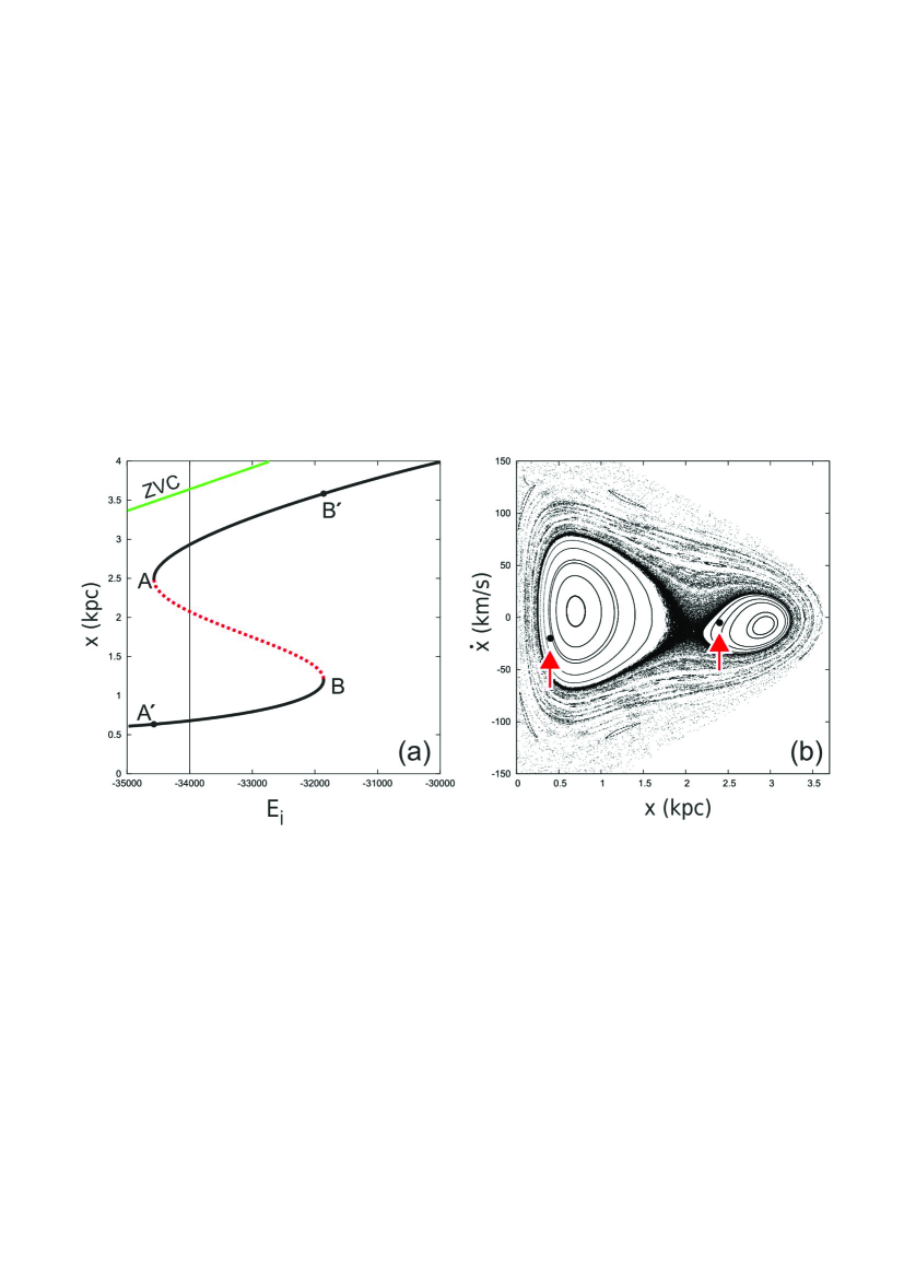
Figure 4: The evolution of the surfaces of section in the ”S” region. In (a) we focus in the ”S” region of the characteristic. Continuous black parts of the curve indicate stability, while dotted (red in the online version) indicate instability. The vertical line at E_J = $-34000$ denotes the energy at which we give the $(x,\dot{x})$ surface of section in (b). With increasing energy between A, A^′ and B, B^′ in (a) the size of the left stability island decreases, while the size of the right one increases. The arrows point to the orbits depicted in Fig. 5.

The (E_J ​​,x) characteristic curve of x1^′ and its bifurcations, as we approach L₄, is given in Fig. 2. Continuous black parts of the curves indicate stability, while dotted (red in the online version) indicate instability. The stable Lagrangian points L₄ and L₅ are at energy E${}_{L_{4,5}}=-22196$ (E_J is always given in units of km² s^-2). L₄ in Fig. 2 is at the local maximum of the curve of zero velocity at the right side of the figure. For the unstable Lagrangian points L₁ and L₂ we have E${}_{L_{1,2}}=-23360$. At this energy we have drawn a solid vertical line in Fig. 2 and we indicate it with an arrow labelled “E${}_{\rm{L_{1}}}$”. The folding of the characteristic curve, which we call “S”, occurs between $-34500<$ E_J $<-31800$ (E_J $\approx-34500$ is the energy at point “A” and E_J $\approx-31800$ is the energy at point “B”).

Since there is no gap or discontinuity in the curve, we consider the whole curve belonging to a single family of periodic orbits, namely the x1^′ . The x1^′ family is stable close to the centre of the model, then it becomes unstable for $-57000<$ E_J $<-50436$ (with a small stability interval $-55000<$ E_J $<-54336$). After that it remains practically stable until the region of the “S”. For E_J $>-31800$ (E_J at point “B”), which we consider as the end of “S”, the upper branch of the characteristic remains stable until the energy E_J $\approx-27000$. Beyond this energy follows a tree of bifurcating families.

Up to this point, the morphological evolution of the periodic orbits along the x1^′ characteristic curve shows an interesting variation. In Fig. 3 we give successively characteristic periodic orbits as the energy increases.

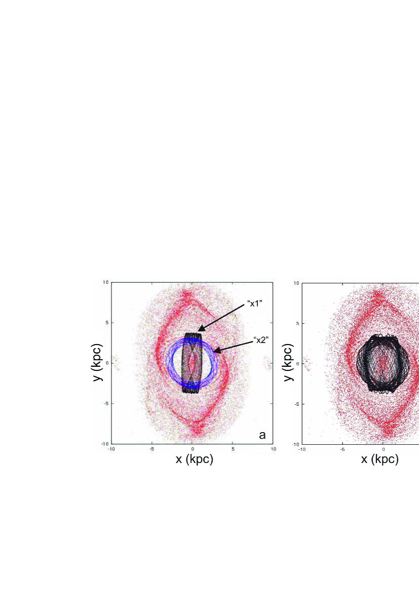
Figure 5: (a) Two characteristic quasi-periodic orbits from the ”S” region of x1^′ supporting a x1 and a x2 flow. Both are at E_J =$-34000$. They are overplotted on our response model. The location of their initial conditions on the $(x,\dot{x})$ surface of section is indicated in Fig. 4b. (b) Three orbits from the chaotic region between the stability islands of Fig. 4b plotted in the central region of the model. Instead of a ring they contribute to the formation of a bulge-like central component.

For E_J $\lessapprox-54000$ the x1^′ orbits are typical x1 ellipses, elongated along the y-axis, as in Fig. 3a. Then for $-54000\lessapprox$ E_J $\lessapprox-38000$ they develop loops at their apocentra (Fig. 3b). As energy increases further, for E_J $>-38000$, the loops at the apocentra vanish again (Fig. 3c) and the morphology of the periodic orbits as we approach the “S” region is as in Fig. 3d. In the “S” region we have three simple periodic orbits at each energy. Two stable and one unstable. At the local maximum of “S” (E_J $\approx-31800$), where the characteristic turns to the left (point “B” in Fig. 2), the orientation of the elliptical periodic orbits starts changing, while, simultaneously, they become unstable. Their major axes lean more and more towards the x-axis as energy decreases. For example the orbit in Fig. 3f, at E_J $\approx-34500$ (point “A ”), the major axis of the periodic orbits is close to the x-axis (minor axis) of the system. In other words, moving along the unstable segment of the characteristic from “B” to “A” we change from a x1- to a x2-like (see e.g. Contopoulos & Grosbøl, 1989) orientation. Then, moving again from E_J $\approx-34500$ to the right along the upper stable branch of “S”, the orbits become stable and of “x2-type” until E_J $\approx-30000$ (Fig. 3g). Beyond this point we have periodic orbits like the one in Fig. 3h. If we plot together successive x1^′ periodic orbits with increasing E_J for E_J $>-28000$ we observe that their major axes start tilting towards the y-axis this time, building a “precessing ellipses pattern” (Patsis, 2009) that can be considered as the backbone of a spiral structure extending to larger distances. The spiral structure is discussed below in section 3.3.

3.1 The ring

In Fig. 4 we focus into the “S” region. The corresponding part of the characteristic is given in Fig. 4a and is included between the energies of “A”, “A^′” and “B”, “B^′’. “A”, “A^′” are at E_J $\approx-34500$ and “B”, “B^′” are at E_J $\approx-31800$. At any energy between, e.g. for E_J $=-34000$, where we have drawn a vertical line in Fig. 4a, we have three periodic orbits. There is always an unstable x1^′ periodic orbit with an intermediate inclination between the stable x1-like (lower part of the characteristic) and the stable x2-like (upper part of the characteristic). The situation can be described as a case of a bistable bifurcation. We can say that at points “A” and “B” we have a direct and an inverse tangent bifurcation.

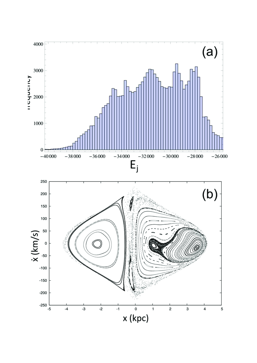
Figure 6: (a) A histogram showing the E_J distribution of the particles with $2.5<r<3.8$ kpc in Fig. 1. (b) The $(x,\dot{x})$ surface of section at E_J =$-32000$, which is a local maximum in (a).

In Fig. 4b we give the $(x,\dot{x})$ surface of section for the energy E_J $=-34000$. It is a typical case of a surface of section in the “S” region. At the centre of the left stability island we have the “x1” periodic orbit, while at the centre of the right stability island we have the x2-like ellipse. The extent of this cross section, as well as of all other similar figures we discuss in our paper, is limited by the zero velocity curve, ZVC (drawn in Fig. 4a). Moving from “B” to “A” along the unstable part of the characteristic in Fig. 4a the area of the right stability island in the surface of section (Fig. 4b) decreases, while the area of the left one increases (Fig. 4b is close to the left border of the “S”). At E_J $\approx-33000$ the width of the chaotic zone between the two ordered regions becomes minimum. The role of the x2-like orbits is even more emphasised as E_J increases beyond “B^′” along the characteristic in Fig. 4b. From “B^′” until E_J $\approx-30000$, the only simple periodic orbits existing are almost perpendicular to the bar. Since they are stable they may attract around them quasi-periodic orbits. If these orbits are populated, they will support a x2 flow.

By inspection of Fig. 3 we can understand the association between the x1^′ periodic orbits and the non-periodic orbits that have been populated in the energy interval of the “S” region (Fig. 4) in order to give the response morphology depicted in Fig. 1. We remind that the initial conditions of the particles in the response model are distributed randomly on a disc of radius 11 kpc and take velocities for circular motion in $\Phi_{0}$ in Eq. (1). The orbits that populate the response model have as initial conditions the positions and the velocities of the test particles at the end of the “time dependent phase” of the model that lasts two rotational periods. In general the x1^′ periodic orbits with small initial $x_{0}$ values ($0.6\lessapprox x_{0}\lessapprox 1.1$) are orientated along the bar (Fig. 3a-d). They are ellipses with their major axes roughly aligned with the major axis of the bar. However, the projections of such orbits from the “S” region, as well as the projections of the quasi-periodic orbits trapped around them, on the major axis of the bar (y-axis) are larger with respect to the bar of the response model, which is included inside the ring (Fig. 1). If we consider quasi-periodic orbits from the left stability island of the surfaces of section in the “S” region they always exceed the size of the ring of the response model. Contrarily, the size of the quasi-periodic orbits from the right stability island is such as to contribute to the formation of the ring, without exceeding the dimensions of the response feature for all E_J values along the “S”. Two quasi-periodic orbits for E_J $=-34000$ that illustrate the above statement are given in Fig. 5a. The locations of the orbits drawn in Fig. 5a in the corresponding stability islands are indicated with arrows in Fig. 4b. The one with the small $x_{0}$ in Fig. 4b is indicated with “x1” in Fig. 5a.

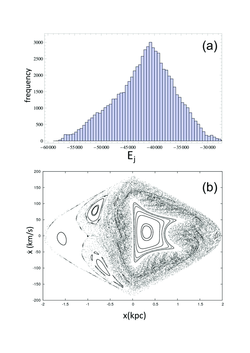
Figure 7: In (a) we give the E_J distribution of particles located at $r<2.5$ kpc in our response model (Fig. 1. The mode is at E_J $=-40750$. In (b) we give the $(x,\dot{x})$ surface of section at the energy of the mode.

Chaotic orbits associated with the unstable branch of the “S” are also not populated in the response model (Fig. 1). In the case depicted in Fig. 4b, such orbits are found in the chaotic zone between the two stability islands. Integrated for 8 rotational periods, they fill the whole central region of the model, including the rather empty areas between the bar and the beginning of the spiral arms, inside the ring. The presence of these orbits in the response model would build a kind of response bulge, instead of a ring. This can be seen in Fig. 5b, where we plot on top of the model, three orbits from the chaotic region with initial conditions $(x,\dot{x})=(2.1,-5)$, $(1.7,-35)$ and $(1.9,-35)$. We observe that they fill the interior of the ring, unlike with what happens in the model. So we can exclude them from the orbits contributing to the response morphology observed in Fig. 1.

The identification of the ring with the x2-like orbits in the “S” region (upper stable branch of “S”) can be verified by considering the distribution of the energies of the particles located in the annulus with $2.5<r<3.8$ kpc in the response model. This is roughly the region of the ring. The radius $r=2.5$ is reaching the inner part of the drawn “x2” orbit in Fig. 5a, while $r=3.8$ reaches the drawn apocentra of the “x1” orbit and the beginning of the spiral arms in the same figure. This energy distribution is given in Fig. 6a. We observe that most of the particles in the ring have energies in the range $-35000\lessapprox$ E_J $\lessapprox-28000$. Particles with E_J $>-28000$ are in quasi-periodic orbits trapped around the stable periodic orbits participating in the beginning of the “precessing ellipses” pattern that builds the spirals (see also Section 3.3 below). Their small contribution in the distribution of the energies in the annulus can be seen at the right part of Fig. 6a for E_J $>-28000$. For E_J $>-32000$ we do not have x1^′ orbits with orientation along the major axis of the bar. This means that if we find in the ring area particles in bar-supporting x1-like orbits they should have E_J $<-32000$. However, as we have seen, we have excluded the presence of x1-like orbits from the lower branch of “S” in the response model, since their size exceeds the size of the ring. So, according to Fig. 6a, if such orbits exist, they will be a minority with E_J $<-34500$. We also note that as we move in the lower branch of the “S” from “A^′” to B (Fig. 4a) the importance of the orbits following the x1 flow decreases. In Fig. 6b we can see the relative importance of the island around the x2-like stable orbit, centred at $(x,\dot{x})=(3.56,-0.1823)$ with respect to the island around the x1-like, centred at $(x,\dot{x})=(1.05,-8.2)$, at E_J $=-32000$. The local maximum of the histogram at about E_J $\approx-32000$ reflects the increasing importance of the stability island around the x2-like stable orbits as we approach this E_J value.

This analysis shows that the observed ring structure in our response model is due to the x2-like orbits that are introduced in the system in the energy range where we have the “S” feature in the characteristic in the bistable region of the central family of periodic orbits. Stable periodic orbits with x2-like orientation exist on the x1^′ characteristic also beyond “B^′” in Fig. 4a (up to E_J $\lessapprox-30000$ and provide to the system the backbone of the ring. The presence of the “S” feature in the characteristic is also associated with the end of the contribution of orbits trapped around stable x1-like orbits aligned with the y-axis to the response morphology of the model. As we have seen in Fig. 6a their contribution to the ring region is minor. Thus, the bar of the model ends practically at the ring. In general up to the energy of “A” and “A^′” (E_J $\approx-34500$) our response model is populated by orbits associated with the lower branch of the x1^′ characteristic. Then we have a jump from “A^′” to “A” and the backbone of our model are the stable orbits along the upper branch of the characteristic.

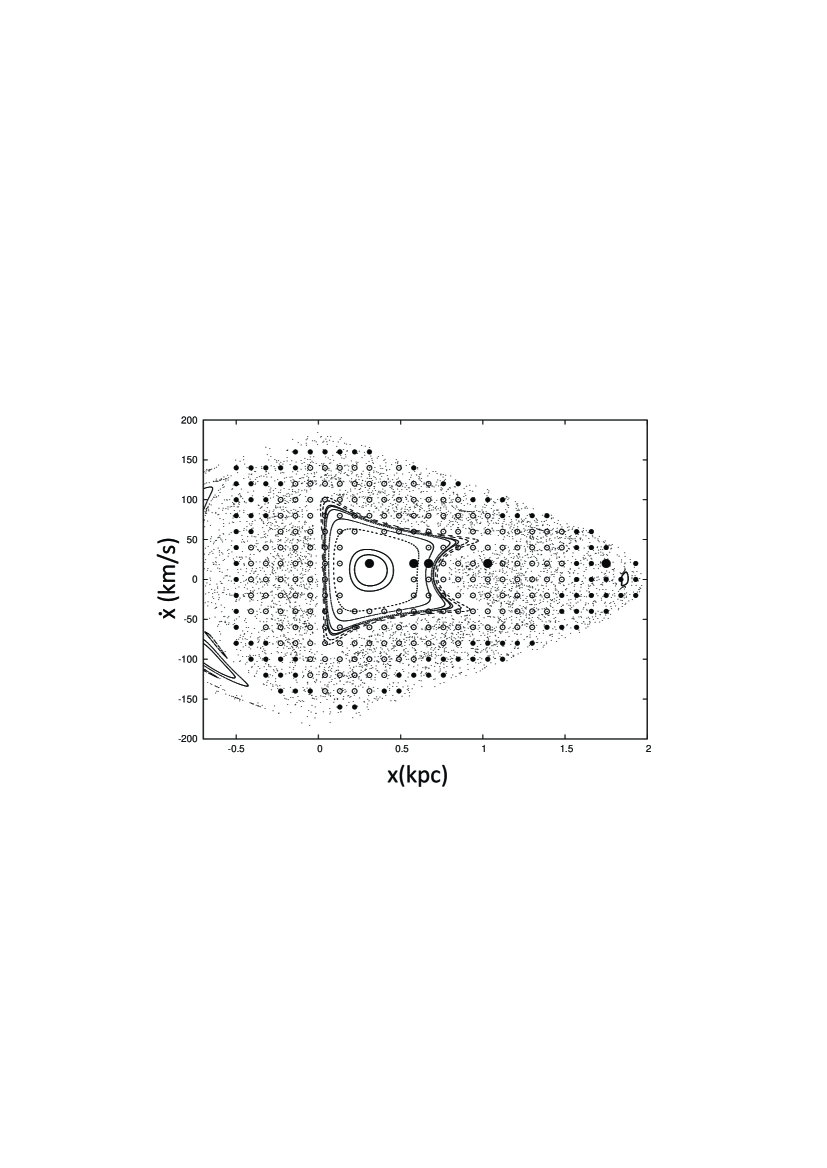
Figure 8: The initial conditions of the integrated orbits on the $(x,\dot{x})$ surface of section at E_J =$-40750$. Small empty bullets correspond to orbits supporting a narrow X feature matching the dimensions of the response bar. Small filled bullets correspond to orbits with an overall X morphology but not matching the dimensions of the bar. The large black bullets indicate the initial conditions of the orbits depicted in Fig. 9.

3.2 The bar

Let us focus now in the response bar and its internal structure. If we confine ourselves to the study of the region of the response model (Fig. 1) with $r<2.5$ kpc, we practically select the region of the bar. The majority of the particles with $r<2.5$ kpc are located in the bar, since the regions to its sides, inside the ring, are regions almost depleted of particles. The energy distribution in this region is given in Fig. 7a. We observe that practically we have particles with E_J $<-30000$ and that the contribution of particles with E_J $>-35000$, i.e. to the right of A, A^′ in Fig. 4a, is small. The mode of the distribution is at E_J $=-40750$.

The main feature of the response bar is an “X” feature, discernible in Fig. 1. We try to understand the mechanism leading to its formation first by investigating the possible contribution of particles with the energy of the mode in Fig. 7a. The $(x,\dot{x})$ surface of section at this energy is given in Fig. 7b. The stability island that dominates in the $x>0$ region is the island of x1^′ ​, which in this energy is x1-like. It is surrounded by a chaotic sea that extends also to $x<0$. At the left side of this chaotic sea we observe two more stability islands belonging to two families of periodic orbits that have a 3:1 character and their characteristic joins the branches of the x1^′ characteristic at energies beyond the “S” in Fig. 2. These orbits do not play any particular role in our study, so we will not deal further with them.

In order to find out the orbits that support the “X” we consider a grid of initial conditions with a step 0.09 in the x- and 20 in the y- direction on the surface of section of Fig. 7b. We integrated the orbits with initial conditions on the nodes of the grid for 30 pattern periods. The initial conditions of the integrated orbits that have been found to give orbits with morphologies relevant to our study are given with filled and empty bullets in Fig. 8. They are encountered for $x>0.5$. In order to demonstrate their morphologies, we present below some characteristic orbital shapes. The large black bullets in Fig. 8 give the initial conditions of five typical orbits that are described in Fig. 9. All of them have $\dot{x_{0}}$=20 km s^-1 ​​, while their $x_{0}$ initial condition increases from Fig. 9a to Fig. 9f. The large bullet inside the innermost invariant curve in Fig. 8 ($x_{0}$=0.31) is given in Fig. 9a and Fig. 9b. In Fig. 9a it is drawn on top of the response model, so that we can see its extent relative to the bar and the ring structure. Its morphology can be seen in another scale in Fig. 9b and is similar to the morphology of a x1-like periodic orbit. For $x_{0}$=0.58, we are still in the area of the stability island (Fig. 9c). The orbit has a boxy character, while we observe the appearance of wings of a X feature being formed towards the apocentra of the orbit. On the central stability island of Fig. 8, but close to its last KAM curve, the hole of the orbit around (0,0) almost vanishes and we have a fully developed X feature in the interior of the orbit. This can be seen in Fig. 9d, with $x_{0}$=0.67. Surrounding the stability island we find a plethora of chaotic orbits, that integrated at least for 10 pattern periods reinforce the appearance of the X. In most cases the X feature was clearly discernible even after integrating the orbit for 30 pattern periods. A typical case is the one given in Fig. 9e. For this chaotic orbit we have $x_{0}$=1.03. The dimensions of this and all other similar chaotic orbits correspond to the dimensions of the response bar we see in Fig. 1. Finally, we find that starting integrating chaotic orbits at the outer border of the chaotic sea, close to the curve of zero velocity, we find again orbits with an X feature embedded in them. However, these orbits are rounder than all other orbits we discussed up to now. A characteristic example can be seen in Fig. 9f ($x_{0}$=1.75). Due to their stubby morphology they do not contribute to the building of the structure of the response bar, since they extend further to its sides.

Using an algorithm similar to that described in Chatzopoulos et al. (2011), we applied simple criteria to characterize the orbits according to their morphology and the degree they support the X-shaped bar of the response model in Fig. 1. In Fig. 8 small bullets indicate only the orbits we find supporting an X feature in the bar region. The empty small bullets indicate narrow orbits that remain confined in the region of the bar ($|x|\lessapprox 1.5$). Such orbits are like those depicted in Fig. 9c,d and e. With filled small bullets we indicate orbits similar to the one in Fig. 9f. They have an interior X-shaped structure, though not as sharp as in Fig. 9e, but their dimensions do not match the dimensions of the bar. In conclusion the X-shaped bar is supported mainly by particles in orbits with initial conditions corresponding to the open bullets in Fig. 8.

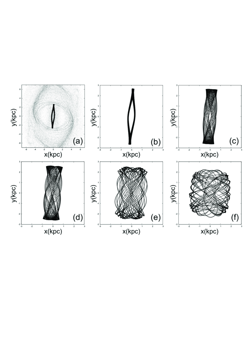
Figure 9: A series of non-periodic orbits with E_J =$-40750$, integrated for 10 pattern periods, that demonstrate the orbital morphologies encountered at this energy. Their initial conditions are indicated with large bullets in Fig. 8. All of them have $\dot{x_{0}}$=20 km s^-1 ​​, while from (a) to (f) their $x_{0}$ are 0.31, 0.31, 0.58, 0.67, 1.03 and 1.75 respectively. The scale of the orbits is the same for panels (b) to (f).

By inspection of Figs. 7,8 and 9 we first realize that the initial conditions supporting the response bar morphology within a certain time are distributed on the surface of section independently of the locations of stability islands or chaotic seas. In general the stability region on Poincaré cross sections that is excluded from participating in the building of a bar is found around the retrograde family x4 (e.g. Contopoulos & Grosbøl, 1989). However, in studies of barred-spiral potentials estimated from near-infrared observations of galaxies (Chatzopoulos et al., 2011; Tsigaridi & Patsis, 2013), it has been realized that there are initial conditions on x1 stability islands, which do not support a particular morphological feature of a bar. On the other hand, we have found that there are initial conditions in the chaotic seas that reinforce a particular bar morphology (Patsis et al., 1997, 2010; Chatzopoulos et al., 2011; Tsigaridi & Patsis, 2013). In the present case quasi-periodic orbits that support part of the wings of an X feature are encountered at the periphery of the stability island of the x1-like periodic orbit. As noticed in Patsis (2005) the morphology of the periodic orbit at the center of an island may differ from the morphology of the quasi-periodic orbits of the outer invariant curves. For example, in cases of elliptical x1-like periodic orbits, the quasi-periodic orbits at the edge of the stability island may support an ansae-type morphology. As we see in Fig. 9 the morphology of the innermost quasi-periodic orbits, which is similar to that of the periodic orbit itself, does not resemble that of an X. On the other hand the integrated for 10-30 pattern periods chaotic orbits with initial conditions in the chaotic sea surrounding the stability island have a morphology matching that of the response bar (cf. Fig. 1 and Fig. 9e).

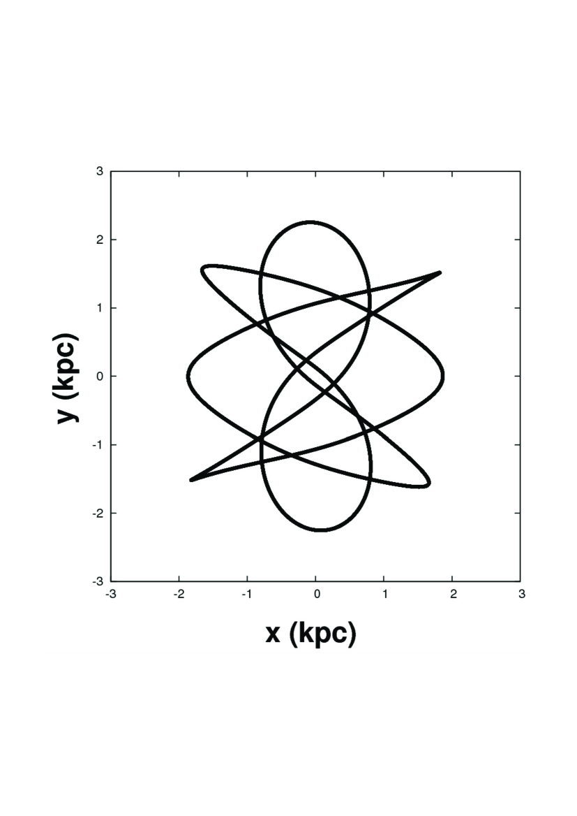
Figure 10: The periodic orbit of multiplicity 3 that has around it a sticky zone with chaotic orbits that have for several tens of pattern periods a morphology similar to the orbit in Fig. 9f.

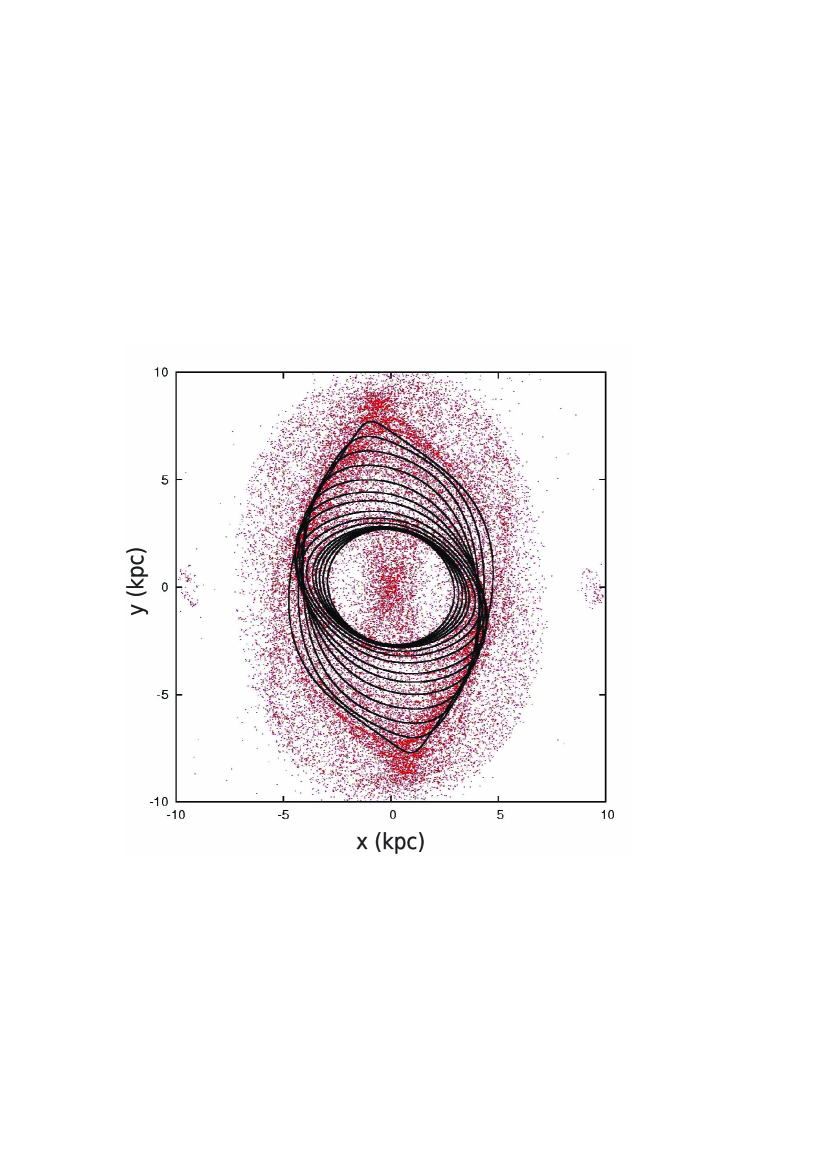
Figure 11: Periodic orbits overplotted on the response model in the range $-34000<$E_J $<-25000$. These orbits are the backbone for the support of the observed spiral pattern and the ring pattern. Energies from inside to outside: $-34000$,$-33500$,$-33000$,$-32500$,$-32000$,$-31000$,$-30000$,$-29000$, $-28000$, $-27500$, $-27000$, $-26500$,$-26000$,$-25500$ and $-25000$.

Since morphologies similar to that of Fig. 9e are encountered by integrating the initial conditions corresponding to the open bullets in Fig. 8, we can compare the area these open bullets occupy with the density of the consequents on the surface of section in Fig. 7b. It becomes apparent that the open bullets symbols are located in the sticky region, i.e. the region with larger density, surrounding the central stability island in Fig. 7b. As regards the study of the orbital morphology it is worth to underline that moving from the center of the stability island outwards and then crossing the surrounding sticky region, we have a smooth morphological transition from narrow non-periodic orbits, along the x-direction, to broader non-periodic orbits, which harbour an X feature. The energy E_J =$-40750$ is the mode of the distribution in Fig. 7a. However, a similar analysis can be done for every E_J roughly in the interval $-45000<$E_J $<-35000$ (practically for energies before the “S” feature). The non-periodic orbits supporting the X are mainly orbits in the sticky zones surrounding stability islands of x1-like periodic orbits.

The zone with the small filled bullets in Fig. 8 is a sticky zone as well, this time around a periodic orbit of multiplicity 3. Its three tiny stability islands can be better seen in Fig. 7b at $(x,\dot{x})\approx(1.8,0)$, $(-0.2,-130)$ and $(-0.4,110)$. In Fig. 10 we give this periodic orbit, so that its morphological relationship with the chaotic orbits in the sticky zone around it (Fig. 9f) becomes apparent.

3.3 The spiral pattern of the model

The response spiral is built by quasi-periodic orbits trapped around elliptical, precessing backwardly with respect to the direction of rotation as energy increases, x1^′ periodic orbits with E_J $\geqslant-28000$. We can see a set of these periodic orbits together with those that form the outer part of the ring in Fig. 11. The mechanism that reinforces the (trailing) spiral arms is a typical “precessing ellipses flow” mechanism (Patsis, 2009). In the energy range $-28000<$E_J ​$<-25000$ the x1^′ stability island occupies practically all the $(x,\dot{x})$ surface of section for $x>0$. The orbits that support the spiral arms are in this case quasi-periodic orbits around x1^′ . The orbital dynamics are similar to those described by Contopoulos & Grosbøl (1986, 1988) for open non-barred spirals. Corotation is placed at 10 kpc, therefore the arms show clear bifurcating branches close the the inner 4:1 resonance. Close to r=8 kpc the x1^′ periodic orbits have cusps and a clear rhomboidal morphology. The bifurcating branches are formed by the congestion of these orbits with more circular orbits further away from the resonance.

4 Discussion

We presented a dynamical mechanism that leads to the formation of a bar with a characteristic X embedded in it. In our model we have simultaneously also the formation of a ring tangent to the ends of the bar. We summarise this result in Fig. 12.

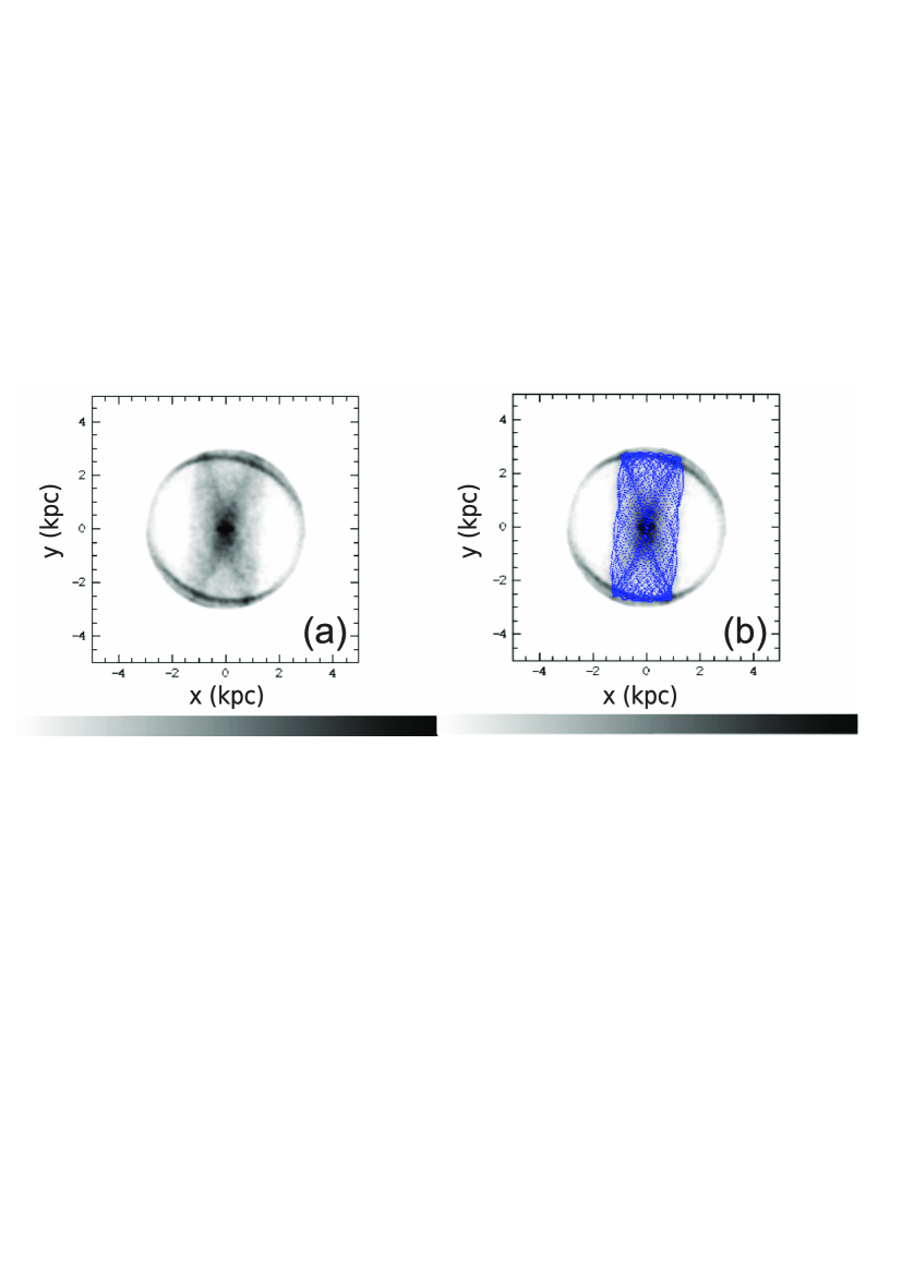
Figure 12: (a) The central region of Fig. 1, which shows the inner part of the ring and the X feature in the bar of the model. (b) Two orbits from the sticky region around the x1^′ stability island in the surface of section for E_J $=-39000$ $(x,\dot{x})$=(0.25,-80) and $(x,\dot{x})$=(1,40) overplotted on the central region of the model. The corresponding x1^′ periodic orbit is x1-like, while the chaotic orbits in this sticky region give the orbital support to the X-shaped feature of the bar.

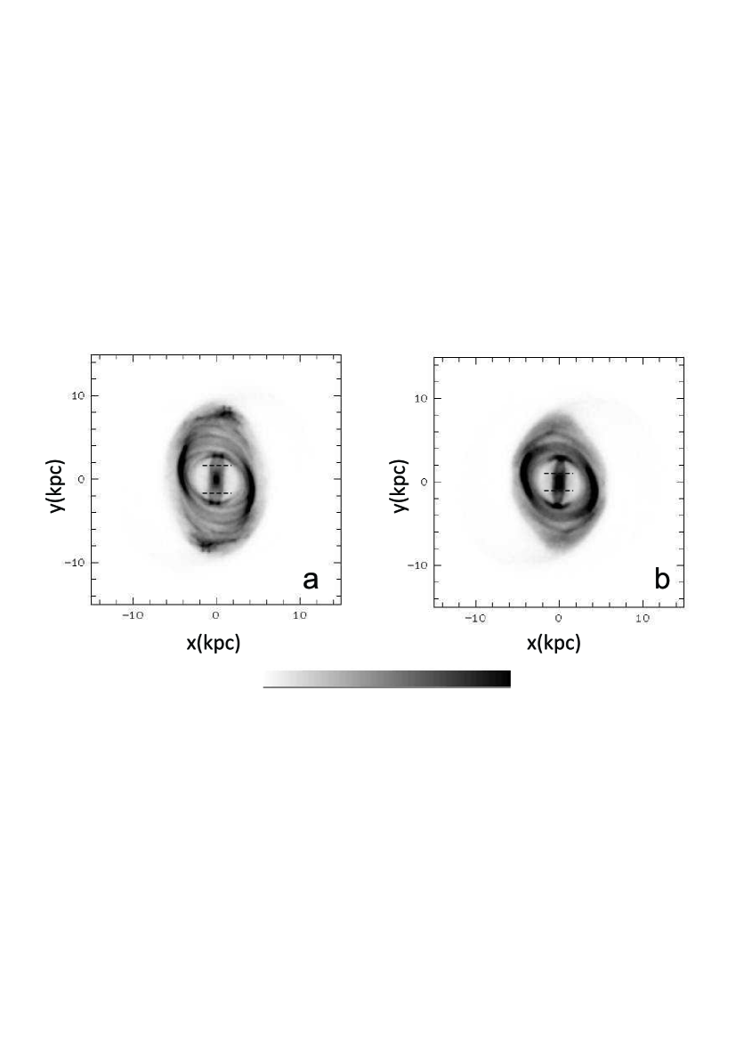
Figure 13: Snapshots from the response models rotating with $\varOmega_{p}$ =13.5 km s^-1 kpc^-1 (a) and 15 km s^-1 kpc^-1 (b). The dashed line segments parallel to the x-axis indicate the height within which extends the X in the two models.

We have used the model with $\varOmega_{p}$ = 11.5 km s^-1 kpc^-1 for presenting this mechanism, because for this pattern speed the X feature extends all over the bar. This facilitates the description of the X morphology. However, it is a feature that we found also in the bar of other response models with $\varOmega_{p}\lessapprox 15$ km s^-1 kpc^-1  ​​, without reaching the end of the bars. We give in Fig. 13 two snapshots from response models with $\varOmega_{p}$ = 13.5 km s^-1 kpc^-1 (a) and 15 km s^-1 kpc^-1 (b) respectively. The maximum distances from the x-axis within which the X extends in these two models are indicated with dashed line segments parallel to the x-axis. The details of the X become less discernible as $\varOmega_{p}$ increases. We observe that the X shrinks with increasing $\varOmega_{p}$ from 11.5 km s^-1 kpc^-1 (Fig. 1) to 13.5 km s^-1 kpc^-1 (Fig. 13a) and then to 15 km s^-1 kpc^-1 (Fig. 13b). This reflects the amount of sticky chaotic orbits that have been populated and participate in the building of the response bars in each case. In the models of Fig. 13, at distances beyond the end of the X feature, the bar has again a backbone of typical x1 orbits until its end.

The characteristic of the central family appears folded over a $\Delta$E_J $\approx 2700$ range, with both x1- and x2-like flows coexisting. The curve folds, but does not break. A similar behaviour has been encountered also in the slowly rotating “Model A2” of a 3D Ferrers bar in Skokos et al. (2002b). The potential we study here is not a pure bar, but a barred-spiral one, allowing both bar and spirals appearing in the stellar response. Due to the low $\varOmega_{p}$, corotation is beyond the end of the spiral arms.

Up to the E_J of “A” and “A^′” our response model is populated by orbits associated with x1-like periodic orbits (quasi-periodic orbits from their stability islands and chaotic orbits from the sticky zones around these islands). For E_J larger than the E_J of “A” and “A^′” our model is populated by orbits associated with the upper branch of the “S”. For the response model it is as “A” and “A^′” coincide on the characteristic. The presence of the bistable bifurcation creates an effective ILR, since it creates a x2-flow. The bistable bifurcation determines the orbits that constitute the backbone of the response model.

The ring still exists for $\varOmega_{p}$ = 13.5 km s^-1 kpc^-1 (Fig. 13a) as a pseudo-ring, or double-ring structure. A rounder inner part seems to be detached from a more elongated x2-like outer part. In our main model (Fig. 1) both parts appear joint forming a unique ring. For $\varOmega_{p}$ = 15 km s^-1 kpc^-1 (Fig. 13b and Tsigaridi & Patsis, 2013) attached to the ends of the bar we have only two density enhancements of “smile” and “frown” morphology. However, a kind of loosely defined pseudo-ring structure appear even in models with $\varOmega_{p}$ = 25 km s^-1 kpc^-1 ​. The ring in our main model is formed by orbits having energies in the middle of the x1^′ characteristic in a (E_J ​​,$x)$ diagram (Fig. 2) and is associated with the folding of this curve. It is formed in the region where the central family of periodic orbits has a bistable character.

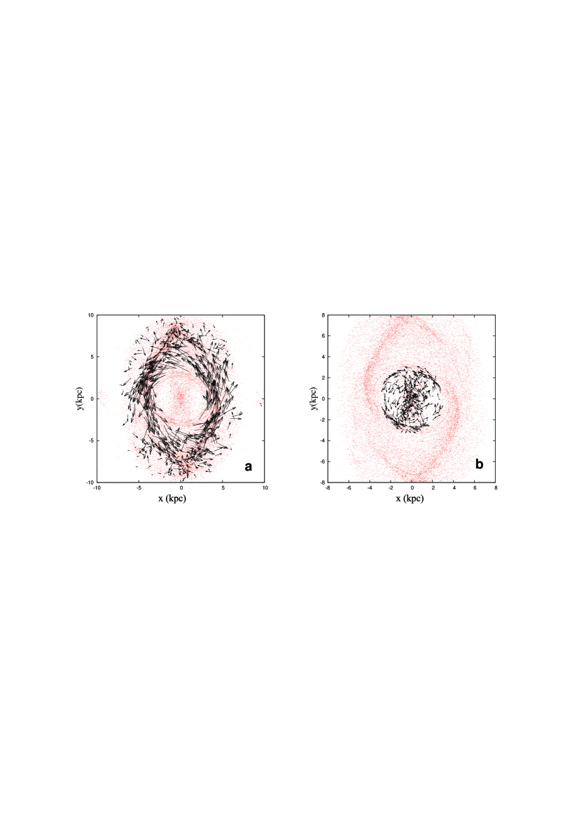
Figure 14: (a) The velocity field of the model outside the ring area indicates a flow around the center of the system. (b) The velocity field of the model in the X-shaped bar region indicates an increased dispersion of velocities.

The ring is formed due to the introduction in the system of a x2 flow, which in fact acts as if we had a usual inner Lindblad resonance region. By surrounding the bar however, it should be characterised as an “inner ring”, usually associated with inner 4:1 or 6:1 resonances (see e.g. Buta, 1986; Byrd et al., 1994; Patsis et al., 2003). Because of their association with inner n:1 resonances with n$\geqq 4$, inner rings are usually orientated along the bar (Buta, 1986). In our case the “inner” ring can be characterised as almost circular or rather elongated towards the minor axis of the bar, depending on the energy level of the orbits we consider as the limit between the x2-flow orbits and the orbits that build the spiral.

The X in the bar is mainly a result of populating sticky orbits around the x1^′ stability islands in the energy range for which we have a backbone of x1-like periodic orbits in our model. In principle this can happen independently of the pattern speed of a model. However, in slowly rotating bars it appears pronounced, as it occupies a larger part of them. In the case of the particular model in this paper the ring is tangent to an “X-shaped” bar. Our model describes a configuration, where ordered and chaotic motion coexist and contribute to the formation of a unique structure.

We note, that despite the 2D character of the present models, due to the morphology of the orbits that build the X, we can observe a characteristic increase in the dispersion of velocities as we cross the ring inwards (Fig. 14). In Fig. 14a the arrows indicate a flow around the center of the model, while in Fig. 14b the orientation of the orbits looks random on the galactic plane. This is to be expected, since the motion of the particles following X-supporting orbits is complicated.

Buta et al. (2007, pg.40), Laurikainen et al (2011, 2014) give several examples of X features in barred-spiral galaxies that are clearly far from edge-on (e.g. NGC 7020, NGC 1527, IC 5240, NGC 4429). The mechanism we propose here, i.e. the population of sticky chaotic orbits around the stability islands of the main family of periodic orbits, suggests an explanation of this morphology. We stress again that the X feature is pronounced in slowly rotating models, but slow rotation does not give the explanation of the feature. The X appears as soon as the bar is built by sticky chaotic orbits in the chaotic zone surrounding the stability islands of x1-like periodic orbits, as well as by quasi-periodic orbits at the outer parts of these islands. The potential in the present paper originates in the estimation of the gravitational field of a late-type barred galaxy. Nevertheless, the X feature is expected to appear also in models for early type barred galaxies, provided that the bar is populated by the kind of sticky chaotic orbits we discuss. We note however, that there are cases of nearly face-on galaxies combining an X feature with a ring (e.g. IC 5240, Buta et al., 2007; Laurikainen et al, 2014). Such galaxies combine the morphological features of the response model of the present study.

Recently Patsis & Katsanikas (2014) investigated the orbital dynamics of 3D Ferrers bars that lead to the formation of boxy features inside the bars in their face-on projections. Despite the fact that the bars in the two cases are approached by different modelling techniques (2D vs. 3D dynamics), the two studies agree on the character of the orbits that build the boxy features. In both cases we deal with sticky chaotic orbits. Similarly with what we find here, also in the 3D models the pool of orbits that are used to build the inner boxes are sticky chaotic orbits around the periodic orbits that constitute the backbones of the bars. However, the 3D modelling allows us to investigate the connection between the X features appearing in the face-on views and the X features appearing in boxy/peanuts edge-on profiles(Patsis & Katsanikas, 2014).

5 Conclusions

The main conclusions of our study refer to the dynamics of slowly rotating barred-spiral models and are enumerated below:

1. The characteristic of the main family in our slowly rotating barred-spiral potential includes periodic orbits that are successively (as E_J increases) x1-like, x2-like, as well as elliptical orbits that precess if plotted at different E_J ​. It is characterised by a folding, which we called the “S” (Fig. 4a). It is a case of two combined saddle-node bifurcations, usually called “bistability”. Along “S” the periodic orbits change their orientation. Slow rotation pronounces this folding. Our response model is populated by x1-like orbits up to the E_J of “A” and “A^′” in Fig. 4a and for larger E_J by orbits associated with the upper branch of the “S”. For the model it is as if we jump from “A” to “A^′” in the characteristic.

2. The abrupt change of the orientation of the response orbits leads to the formation of a ring in the middle of the characteristic, at the “S” region. The ring does not extend along the bar, as is the usual orientation of inner rings, but it is rather inclined towards the x-axis. We have effectively a x2 region beyond the end of the bar. The orientation and morphology of the ring resembles more that of nuclear rings.

3. Bars built mainly by sticky orbits around the stability islands of the central family of periodic orbits have a boxy structure that harbours an X feature in it. In the class of barred-spiral models we consider in the present study, the slower the pattern speed of the model, the greater is the importance of the X-feature for the overall morphology of the bar, since it occupies a larger fraction of it. However, the dynamical mechanism behind it is encountered in response models within a larger range of pattern speeds, since it depends on the amount of sticky chaotic orbits that populate the bar.

Acknowledgements

We thank Prof. G. Contopoulos for fruitful discussions and very useful comments and the referee, Dr. Pertti Rautiainen, for his comments and suggestions, which contributed in improving the paper. This work has been partially supported by the Research Committee of the Academy of Athens through the project 200/823.

References

- Angeli et al (2003) Angeli D., Ferrell J.E. Jr., Sontag E.D., 2003, Proc. Nat. Acad. Sci. 101, 1822
- Boonyasait (2003) Boonyasait V., 2003, PhD Thesis, University of Florida
- Buta (1986) Buta R., 1986, ApJSS 61, 609
- Buta et al. (2007) Buta R.J., Corwin H.G. Jr., Odewahn S.C., 2007, The de Vauvouleurs Atlas of Galaxies, Cambridge University Press
- Byrd et al. (1994) Byrd G., Rautiainen P., Salo H., Buta R., Crocker D.A., 1994, AJ 108, 476
- Chatzopoulos et al. (2011) Chatzopoulos S., Patsis P. A., Boily C.M., 2011, MNRAS 416, 479
- Combes & Elmegreen (1993) Combes F., Elmegreen B.G., 1993, A&A 271, 391
- Contopoulos (1980) Contopoulos G., A&A 81, 198
- Contopoulos (2004) Contopoulos G., 2004, ”Order and Chaos in Dynamical Astronomy”, Springer
- Contopoulos & Grosbøl (1986) Contopoulos G. & Grosbøl P., 1986, A&A 155, 11
- Contopoulos & Grosbøl (1988) Contopoulos G. & Grosbøl P., 1988, A&A 197, 83
- Contopoulos & Grosbøl (1989) Contopoulos G. & Grosbøl P., 1989, A&ARv, 1, 261
- Contopoulos & Papayannopoulos (1980) Contopoulos G. & Papayannopoulos T., 1980, A&A 92, 33
- Elmegreen & Elmegreen (1985) Elmegreen B.G., Elmegreen D.M., 1985, ApJ 288, 438
- Font et al. (2014) Font J., Beckman J., Zaragoza-Cardiel J., Fathi K., Epinat B., Amram P., 2014, ApJSS 210, 2
- Gottesman (1982) Gottesman S.T., 1982, AJ 87, 751
- Junqueira et al (2013) Junqueira T.C., Lépine J. R. D., Braga C. A. S., D. A. Barros D. A., 2013, A&A 550, 91
- Kaufmann & Patsis (2005) Kaufmann D.E., Patsis P.A. 2005, ApJ 624, 693
- Kranz et al (2003) Kranz T., Slyz A., Rix H-W., 2003, ApJ 586, 143
- Laurikainen et al (2011) Laurikainen E., Salo H., Buta R., Knapen J. H., 2011, MNRAS 418, 1452
- Laurikainen et al (2014) Laurikainen E., Salo H., Athanassoula E., Bosma A., Herrera-Endoqui M., 2014, MNRAS 444, L80
- Lynch (2007) Lynch S., 2007, “Dynamical Systems with Applications using Mathematica”, Birkhäuser, Boston
- Lynden-Bell (1979) Lynden-Bell D., 1979, MNRAS 187, 101
- Martos et al (2004) Martos M., Hernandez X., Yanez M., Moreno E., Pichardo B., 2004, MNRAS 350L, 47
- Pasha & Polyachenko (1994) Pasha I.I., Polyachenko V.L., 1994, MNRAS 266, 92
- Patsis (2005) Patsis P.A., 2005, MNRAS 358, 305
- Patsis (2009) Patsis P.A., 2009, in Chaos in Astronomy, Contopoulos G., Patsis P.A. (eds.), Springer Verlag, Heidelberg. pp 33-44
- Patsis et al. (1991) Patsis P. A., Contopoulos G., Grosbøl P., 1991, A&A, 243, 373
- Patsis et al. (1997) Patsis P. A., Athanassoula E., Quillen A. C., 1997, ApJ, 483, 731
- Patsis et al. (2009) Patsis P. A., Kaufmann, D. E., Gottesman S.T., Boonyasait, V., 2009, MNRAS 394, 142
- Patsis et al. (2010) Patsis P. A., Kalapotharakos C., Grosbøl P., 2010, MNRAS 408, 22
- Patsis et al. (2002) Patsis P. A., Skokos Ch., Athanassoula E., 2002, MNRAS 337, 578
- Patsis et al. (2003) Patsis P. A., Skokos Ch., Athanassoula E., 2003, MNRAS 346, 1031
- Patsis & Katsanikas (2014) Patsis P. A., Katsanikas M., 2014, MNRAS 445, 3546
- Petrou & Papayannopoulos (1986) Petrou M., Papayannopoulos T., 1986, MNRAS 219 157
- Rautiainen et al. (2008) Rautiainen P., Salo H., Laurikainen E., 2008, MNRAS 388, 1803
- Skokos et al. (2002a) Skokos Ch., Patsis P. A., Athanassoula E., 2002a, MNRAS 333, 847
- Skokos et al. (2002b) Skokos Ch., Patsis P. A., Athanassoula E., 2002b, MNRAS 333, 861
- Strogatz (2014) Strogatz S.H., 2014, “Nonlinear Dynamics and Chaos: With Applications to Physics, Biology, Chemistry and Engineering”, Westview Press
- Tsigaridi & Patsis (2013) Tsigaridi L., Patsis P.A., 2013, MNRAS, 434, 2922 (paper I)