Relaxation processes in a system with logarithmic growth

Abstract

We discuss relaxation and aging processes in the one- and two-dimensional $ABC$ models. In these driven diffusive systems of three particle types, biased exchanges in one direction yield a coarsening process characterized in the long time limit by a logarithmic growth of ordered domains that take the form of stripes. From the time-dependent length, derived from the equal-time spatial correlator, and from the mean displacement of individual particles different regimes in the formation and growth of these domains can be identified. Analysis of two-times correlation and response functions reveals dynamical scaling in the asymptotic logarithmic growth regime as well as complicated finite-time and finite-size effects in the early and intermediate time regimes.

I Introduction

Emerging patterns due to coarsening are encountered in a huge variety of systems Cro93 , ranging from magnetic systems Bra94 ; Hen10 to complex fluids Cat15 and from competition in bacterial colonies Szo14 ; Rom13 to opinion dynamics in social systems Cas09 . The general understanding of phase ordering kinetics Pur09 is well developed for a range of systems, notably those that are curvature driven and where the size of a typical domain increases with the square root of time. Power-law growth is also observed in other instances, as for example in systems with a conserved order parameter undergoing Ostwald ripening Voo85 .

However, coarsening processes in more complex systems can yield a domain growth much slower than the algebraic growth observed in the simpler situations Cug14 . Systems where a logarithmic growth of the form $\sim(\ln t)^{1/\psi}$ is expected include spin glasses and disordered ferromagnets. In general, it is challenging, both in experimental and numerical studies, to reach the very long timescales needed to fully access the asymptotic regime. This has been a vexing issue of many years for spin glasses. On the other hand, disordered ferromagnets, while still being challenging systems, are more easily dealt with in that regard, and over the years a range of studies focusing on elastic lines in disordered media Kol05 ; Noh09 ; Igu09 ; Mon09 and on disordered Ising systems Rao93 ; Aro08 ; Par10 ; Cor11 ; Cor12 ; Par12 ; Cor13 ; Man14 , including the one-dimensional random field Ising model Fis01 ; Cor02 , have shown that the asymptotic growth regime is indeed non-algebraic and compatible with a logarithmic growth of the domains.

A logarithmically growing length scale is not restricted to disordered systems, but is also encountered in some systems dominated by dynamical constraints rather than by quenched disorder Eva02 . Anomalous coarsening with logarithmic domain growth has been identified in a variety of situations with dynamical constraints, as for example in the $ABC$ model introduced by Evans et al Eva98a ; Eva98b , where three different particle types swap places asymmetrically, in the model discussed by Lahiri and Ramaswamy Lah97 ; Lah00 , where two sublattices are considered with two types of particles on each sublattice, or in the driven two-lane particle system studied by Lipowski and Lipowska Lip09 . Among these models, the one-dimensional $ABC$ model has enjoyed much attention in recent years Cli03 ; Bod08 ; Ayy09 ; Led10a ; Led10b ; Bar11a ; Ber11 ; Bar11b ; Bod11 ; Coh11 ; Ger11 ; Coh12a ; Ger12 ; Coh12b ; Afz13 ; Ber13 ; Coh14 ; Mis14 , due to its unique properties combined with its amenability to exact calculations in some special cases. Thus the $ABC$ model provides an opportunity to study exactly the long-range correlations in a system undergoing a non-equilibrium phase transition as well as to elucidate ensemble inequivalence far from equilibrium.

Whereas most of the papers on the $ABC$ model focused on steady-state properties, only few studies directly addressed the coarsening process, the logarithmic growth and other issues related to this anomalous slow process. After having identified the anomalous slow domain growth in the $ABC$ model, Evans et al Eva98b proposed a simplified interface model where domains rather than individual sites are updated. In Kaf00 slow coarsening was shown to also exist in a two-dimensional version of the $ABC$ model. Finally, in Afz13 the focus was on the interface model in one dimension whose study provided some insights into aging and dynamical scaling in presence of a logarithmically growing length.

In this paper we aim at further elucidating slow coarsening and relaxation processes in both the one- and two-dimensional $ABC$ models. In order to do so, we study a range of different quantities (the time-dependent space-time correlation function and the length scale obtained from it, two-times quantities like the autocorrelation and response functions, as well as the mean displacement of individual particles during the coarsening process) that allow us to gain a good understanding of the non-equilibrium processes taking place in this system. We thereby discuss different regimes that can be identified during the coarsening process. The effects of the system size and of the swapping rate on the domain ordering are discussed.

The paper is organized in the following way. In the next section we recall the model, both in one and two space dimensions, and introduce the quantities that we study in the remainder of the paper. Section III is devoted to a discussion of the time-dependent lengths that govern the coarsening process. Whereas asymptotically the length in the horizontal direction increases as a logarithm of time, complicated early time regimes emerge, depending on the degree of asymmetry and the extent of the system. Additional insights are provided by the mean displacement of individual particles. In section IV we study two-times quantities. Whereas the autocorrelation exhibits obvious dynamical scaling properties, a complicated response of the system to perturbations (realized through a sudden change of the swapping rates) is observed. We summarize our results in the final section.

II Model and quantities

We consider particles of three different types (called $A$, $B$, and $C$) moving on a two-dimensional lattice with $L\times M$ sites and periodic boundary conditions in both the $x$- and $y$-direction. Whereas in the $y$-direction all exchanges are symmetric and happen with rate 1, in the $x$-direction a bias is introduced that yields an asymmetry in the exchanges and, concomitantly, an asymmetrical diffusion of the particles Kaf00 . This is achieved by allowing exchanges between particles on neighboring sites in the horizontal direction to take place with the following rates:

$$AB\overset{q}{\underset{1}{\rightleftarrows}}BA~{},$$

$$BC\overset{q}{\underset{1}{\rightleftarrows}}CB~{},$$

$$CA\overset{q}{\underset{1}{\rightleftarrows}}AC~{},$$ (1)

i.e. a $B$ particle and an $A$ particle to the right of the $B$ particle will swap places with rate 1, whereas the same two particles will swap places with some rate $q<1$ in case their order is different. Unbiased exchanges are of course recovered when $q=1$. The driven diffusive motion that results when $q<1$ entails phase separation and the formation of ordered domains in the form of vertical stripes Kaf00 that are arranged in repetitions of the sequence $ABC$ where $A$ stands for a domain occupied by a majority of $A$ particles.

For comparison, we also simulate the $ABC$ model on a ring composed of $L$ sites Eva98a ; Eva98b where the same biased rates are used as for the horizontal direction in the two-dimensional model.

Most of the data discussed below have been obtained for systems with $L=600$. We carefully checked that this horizontal length is big enough so that it does not yield finite-size effects for the times accessed in our simulations.

In all our simulations we consider fully occupied lattices where initially every species occupies exactly one third of the lattice sites chosen at random. This is in fact a special situation in one space dimension, as detailed balance is then fulfilled Eva98a so that the system relaxes to an equilibrium steady state: in case of identical coverage of the lattice by each of the species, a Hamiltonian with long-range interactions can be derived. However, as soon as the particle densities are not the same for all three species, detailed balance is broken in one dimension and the steady state is a non-equilibrium steady state. The phase transition between the ordered phase for $q<1$ and the disordered phase at $q=1$ (in the large volume limit) then becomes a non-equilibrium phase transition Cli03 which has been at the center of some of the recent studies dealing with the $ABC$ model. For the two-dimensional model, however, detailed balance is always broken, even when the three particle densities are identical, and the steady state is always a non-equilibrium steady state Kaf00 .

We are using a standard scheme for our simulations where we randomly select a neighboring pair of sites. In case the particles occupying these sites belong to different species, they are exchanged with the direction-dependent rates given above. We define a time step as $N$ such proposed updates, where $N=L\times M$ is the total number of sites forming the lattice.

Every lattice site $\bf{x}$ can be characterized by a time-dependent three-state Potts variable $p({\bf x},t)$. Using that description, an exchange of particles occupying neighboring sites corresponds to updating the values of the Potts variables characterizing these sites. In this way it is also very easy to write down expressions for the quantities measured in our simulations.

A central quantity for our analysis is the equal-time spatial correlation

$$C({\bf r},t)=\left<\frac{1}{N}\sum_{{\bf x}}\delta_{p({\bf x},t),p({\bf x}+{\bf r},t)}\right>-\frac{1}{3}~{},$$ (2)

where $\delta$ is the Kronecker delta. The sum is over all lattice sites, and $\left<\cdots\right>$ stands for an ensemble average over both initial configurations and noise realizations. The subtraction by $\frac{1}{3}$ assures that in an infinite system $C({\bf r},t)$ goes to zero when $\left|{\bf r}\right|\longrightarrow\infty$.

The space-time correlation (2) allows the extraction of a time-dependent correlation length. As we use different swapping rates in horizontal and vertical directions, the spatial correlation, and therefore the correlation length, is direction dependent. For example, in the horizontal direction a time-dependent length $L_{x}(t)$ can be obtained in a standard way by determining the intersection of the normalized correlation $C(\left|x\right|,t)/C(0,t)$ with a constant function $C_{0}$:

$$C(L_{x}(t),t)/C(0,t)=C_{0}~{}.$$ (3)

We carefully checked that the qualitative features of $L_{x}(t)$ discussed below do not depend on the chosen value of $C_{0}$. The data shown in the following have been obtained for $C_{0}=1/3$. Alternatively, a time-dependent horizontal length can be obtained by measuring the average horizontal extent of a connected cluster formed by particles of the same species. We carefully compared the two lengths and found that both lengths are completely equivalent and show the same qualitative features. A vertical length can be obtained from the vertical extent of these clusters.

Two-times quantities have been shown in many studies to be very valuable when investigating the non-equilibrium properties of systems relaxing to a steady state Hen10 . The two-times autocorrelation function

$$C(t,s)=\left<\frac{1}{N}\sum_{{\bf x}}\delta_{p({\bf x},t),p({\bf x},s)}\right>-\frac{1}{3}~{}$$ (4)

compares the configurations at the waiting time $s$ with that at the observation time $t>s$. Important insights can also often be obtained from two-times response functions. For the model discussed here the only control parameter that can be used to perturb the system is the swapping rate $q$. Therefore we use as our perturbation a sudden global change of $q$ from some initial value $q_{i}$ to some final value $q_{f}$ at time $s$ after preparing the system. For times $t>s$ we then monitor how the system relaxes to the final steady state by measuring the time-dependent horizontal length $L_{x,p}(t,s)$ of the perturbed system. Of particular interest is the difference Afz13

$$M(t,s)=\left|L_{x,p}(t,s)-L_{x}(t)\right|$$ (5)

between the length measured in the perturbed system and that measured in the system where $q=q_{f}$ at all times.

All the quantities mentioned up to now do not provide direct information on the behavior of individual particles. In order to probe the system at this more microscopic level, we tag individual particles and follow their motion. From the resulting individual trajectories we determine the displacement of each particle from its initial position as a function of time. In the two-dimensional system particles of course move in both dimensions, but the vertical motion is rather trivial as exchanges between neighboring particles of different types always take place. For that reason we only discuss the mean displacement of the particles in the horizontal direction:

$$d(t)=\left<\frac{1}{N}\sum\limits_{i=1}^{N}\left|x_{i}(t)-x_{i}(0)\right|\right>~{},$$ (6)

where $x_{i}(t)$ is the horizontal coordinate of the position vector ${\bf r}_{i}(t)$ of particle $i$ at time $t$, whereas $x_{i}(0)$ is the horizontal coordinate of the position of the same particle in the initial configuration.

III Time-dependent length scale

As discussed in the previous section, in two space dimensions we can extract both a horizontal and a vertical length. Due to the anisotropy of the system, these lengths are not identical. In order to directly compare with the one-dimensional $ABC$ model, we mostly focus in the following on the length in the horizontal direction.

Figure 1: (Color online) Time-dependent length $L_{x}(t)$ for (a) $q=0.8$ and (b) $q=0.2$. Systems with different extents in the $y$-direction are considered, ranging from 1 (top curve for large $t$) to 100 (bottom curve for large $t$) lines. The length is obtained from the space-time correlation function $C(\left|x\right|,t)$ in the horizontal direction. Some configurations are shown for the $600\times 100$ system. For the larger systems the length is extracted after averaging over more than 1000 independent realizations, whereas for the one-dimensional system the ensemble average is performed over 16000 independent runs.

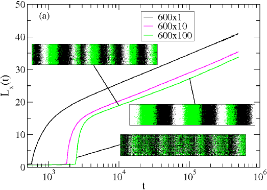
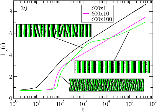
Fig. 1 shows the horizontal length $L_{x}(t)$ for systems of up to 100 lines and two very different values of $q$, namely $q=0.8$ in Fig. 1a and $q=0.2$ in Fig. 1b. The value $q=0.8$ is close to the value $q=1$ for unbiased exchanges. This closeness to $q=1$ gives raise to a very slow initial onset of the ordering process, and it takes for a system composed of 10 or more lines around 2000 time steps before a growth in $L_{x}(t)$ can be observed. This is different for the case of strong bias, $q=0.2$, where ordering emerges already after less than 100 time steps. Once ordering sets in for $q=0.8$, it rapidly yields the formation of ordered stripes (see the configurations in Fig. 1a for the system with 100 lines). These stripes initially contain a large number of particles from the minority species. When the domains are well formed, a coarsening process sets in that reveals itself by a logarithmic growth of $L_{x}(t)$. For systems with $q=0.2$ and only a few lines, this behavior is qualitatively very similar to the behavior encountered for $q=0.8$, the main differences being the earlier onset of ordering and the rapid formation of a large number of well ordered domains in form of stripes. Once these domains are formed, they coarsen very slowly and grow only logarithmically with time. Interestingly, for systems with a larger vertical extent (see the data for the $600\times 100$ system in Fig. 1b) an intermediate regime shows up after the onset of ordering but before the domain coarsening. The nature of this regime, which is characterized by an accelerated increase of $L_{x}(t)$ followed by a strong slowing down of the growth process, is revealed when inspecting the typical configurations shown in Fig. 1b and Fig. 2. In the early stages of the ordering process, clusters merge and grow in vertical direction until they reach from bottom to top. This vertical growth, which gives raise to a transient algebraic growth regime, yields initially some defects that need to be eliminated before entering the logarithmic coarsening regime. Consequently, the asymptotic growth regime sets in much later than for the systems with only a few lines.

Figure 2: (Color online) Snapshots of a system with $q=0.2$ composed of $600\times 100$ sites for six different times between $t=60$ and $t=720$. Only one of the three particle types is shown for clarity. The times shown span the initial regime of domain formation, the regime where the domains merge and expand in vertical direction, and the regime where defects are eliminated and the straight stripes are forming, after which the system enters the logarithmic coarsening regime. The circle highlights one instance where the misalignment of merging domains and the following expansion in the vertical direction yields bended domains as well as a $Y$-shaped connection.

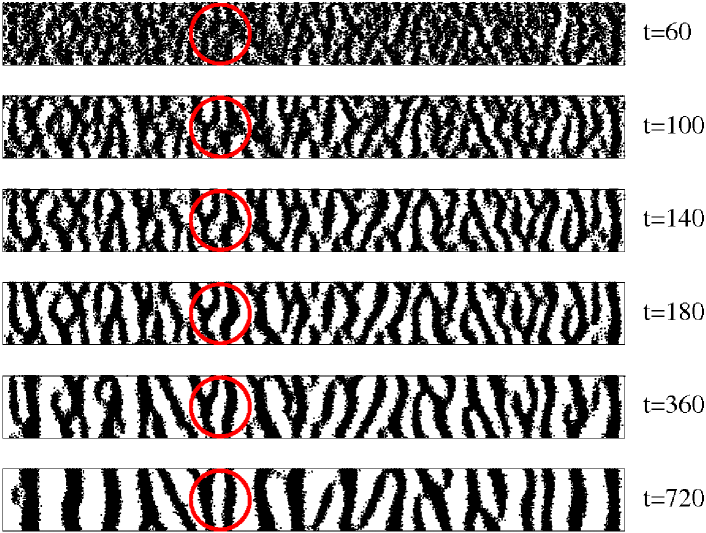
In order to gain a more microscopic picture of the processes taking place in the pre-asymptotic regimes, we show in Fig. 2 six different snapshots, with times between $t=60$ and $t=720$, for a system with $600\times 100$ sites and $q=0.2$. Only one of the three particle types is shown, as this allows to better see the processes taking place in the system. The initial ordered clusters develop at random positions and rapidly merge into anisotropically ordered domains where the growth in vertical direction is much faster than in horizontal direction. When merging, these vertically rapidly growing domains are not always well aligned, which yields defects as for example bended stripes or $Y$-shaped connections. The red circles in Fig. 2 indicate the formation and subsequent evolution of some defects. Once these imperfect stripes are formed, a regime sets in where the defects are eliminated. At $t=720$ only few defects are left and most of the stripes, which have become much straighter, extend through the whole system in vertical direction. The asymptotic logarithmic growth regime is fully accessed only after all these defects have been eliminated.

Figure 3: (Color online) The same as in Fig. 1, but now for systems with a larger extent in $y$-direction. The data result from averaging over at least 1000 independent runs. The inset in (b) shows the same data as in the main panel, but now in a log-log plot. The full solid line indicates the intermediate algebraic growth regime with an exponent 0.25(1).

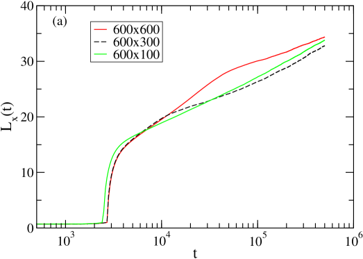
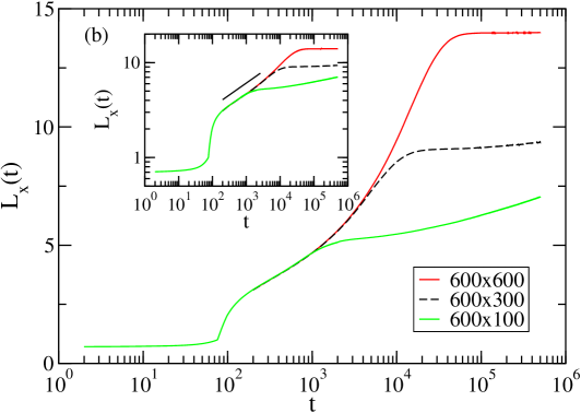
Fig. 3 shows the behavior of $L_{x}(t)$ when further increasing the number of lines. We first note from Fig. 3b that for $q=0.2$ the intermediate regime lasts longer the larger the vertical extent of the system is, as it takes longer to form the parallel stripes spanning the system. The approximate power-law growth connected to this regime is revealed in the log-log plot shown in the inset. The full solid line indicates that this growth is governed by an effective exponent of 0.25(1). For $q=0.8$, see Fig. 3a, the intermediate regime also emerges for larger systems in $y$-direction. In fact the same regimes exist for all values of $q$ and only the characteristic extent in $y$-direction needed for the existence of the intermediate regime depends on $q$.

Figure 4: (Color online) Time evolution of the vertical length $L_{y}(t)$ for (a) $q=0.8$ and (b) $q=0.2$. The systems all have 600 sites in horizontal direction, but different extents in $y$-direction. The different regimes indicated by numbers in (b) for the system with $600\times 600$ spins are discussed in the main text.

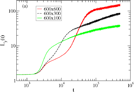
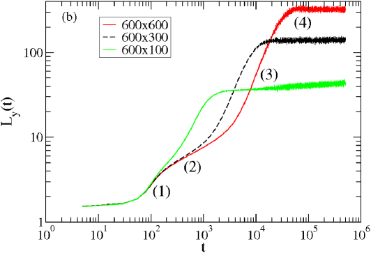
The different regimes identified from our analysis of $L_{x}(t)$ also reveal themselves through characteristic features in the vertical length, as shown in Fig. 4 where we plot the average vertical extent of connected clusters. Focusing first on Fig. 4b, we note that the initial domains grow rapidly in the early time regime (1), before entering the intermediate regime (2) where the merging of ordered clusters yields defect structures that needs to be eliminated. The growth regime (3) then corresponds to the elimination of these defects and the straightening of the stripes. The asymptotic regime (4), characterized by a logarithmic growth in horizontal direction, reveals itself in the following very slow increase of $L_{y}(t)$. All these features are also observed in Fig. 4a for $q=0.8$, albeit less pronounced and separated by more gradual transitions.

In Eva98b and Kaf00 interface models with simplified dynamics were proposed both in one and two space dimensions in order to capture the long time behavior. These models assume instantaneous moves of particles from one domain to another of the same type, with a rate that depends on $q$ as well as on the width of other stripes located between these two domains. In doing so, one neglects that in the original $ABC$ model particles need a finite amount of time to cross these intermediate stripes.

Figure 5: (Color online) Time-dependent length $L_{x}(t)$ vs $\ln t$ for various values of the bias $q$ in a system composed of $600\times 10$ sites. The values of $q$ increase from top to bottom. Plotting $|\ln(q)|L_{x}(t)$ on the $y$-axis yields in all cases curves with slopes $\kappa=0.89(2)$.

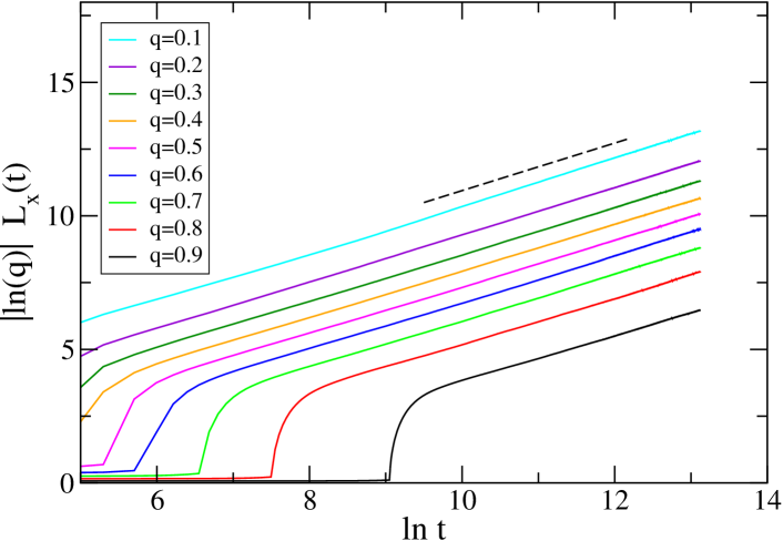
For the $600\times 1$ and $600\times 10$ systems we are able to access in the microscopic model the asymptotic growth regime for all values of $q$ between 0.9 and 0.1. In agreement with what has been observed for the interface model Eva98b ; Afz13 , we find also for the microscopic model that the plot of $L_{x}(t)$ versus $\ln t$ yields a slop that depends on $q$ in the following way:

$$L_{x}(t)=\kappa\,\ln t/\left|\ln q\right|$$ (7)

with $\kappa=0.89(2)$ for both system sizes. This is illustrated in Fig. 5 for the system containing $600\times 10$ sites. The value of $\kappa$ is much smaller than the value $\kappa\approx 2.0$ found for the interface model in one dimension Afz13 , in agreement with the expectation that the simplified dynamics in that model leads to a change in the value of the unit of time.

Figure 6: (Color online) Mean displacement in horizontal direction of particles in a system composed of $9000\times 100$ sites in (a) a log-log plot and (b) a log-linear plot. The values of $q$ decrease from top to bottom. Results for different values of $q$ are shown. For $q=1$ a square-root increase of $d$ is observed, as expected for an unbiased random walk. For $q<1$ a crossover to a regime where the displacement only grows logarithmically with time is encountered. These data result from averaging over 16 independent runs.

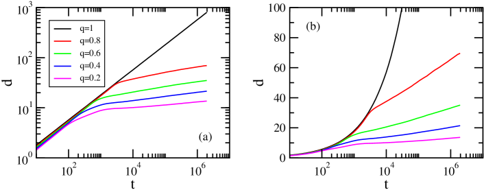
Taking a more microscopic point of view, we can record the trajectories of the individual particles and determine in this way their typical motion. Fig. 6 shows the mean displacement in horizontal direction of particles moving in systems with 100 lines. As is the case for $L_{x}(t)$, two well-separated regimes can also be identified for large $q$ values when studying this quantity, whereas for smaller $q$ values indications of an additional intermediate regime are seen. Initially, the mean displacement for every $q$ displays the same square-root behavior as for $q=1$. This indicates an unbiased diffusion regime at short times before the formation of stripes sets in. For large values of $q$, a crossover to a logarithmic time dependence takes place once the stripes are formed. Note that this transition is very sharp for $q=0.8$. For the smaller values of $q$, see for example the data for $q=0.2$, a more gradual transition is observed, in agreement with the more complicated behavior of $L_{x}(t)$ for that case. This gradual transition is related to the elimination of defects in the horizontal direction and the subsequent straightening of the stripes. During this process particles can move more freely in vertical direction than in horizontal direction, as due to the defect structures not every particle in a stripe is surrounded in vertical direction by particles of the same type. Consequently, it happens that a particle at the borderline region of an imperfect stripe lands after moving only a few steps in vertical direction in another layer where it finds itself the midst of a domain of another species, thus allowing it to then move in the horizontal direction. As shown by our data, this process yields a displacement in horizontal direction that is slower than diffusive and faster than logarithmic.

Figure 7: (Color online) Mean displacement of particles on the one-dimensional ring with 9000 sites in (a,c) a log-log plot and (b,d) a log-linear plot. At very large times, the values of $q$ decrease from top to bottom. In (a,b), following the rules of our model, a particle is not exchanged with a neighboring particle of the same type, yielding for unbiased exchanges with $q=1$ an effective sub-diffusive behavior $d\sim t^{1/4}$. When also allowing for exchanges between particles of the same type, see (c,d), the square-root increase of a random walk prevails. Irrespective whether or not exchanges between like particles are allowed, a crossover to a logarithmic increase is observed for $q<1$. The curves result from an average over 200 independent runs.

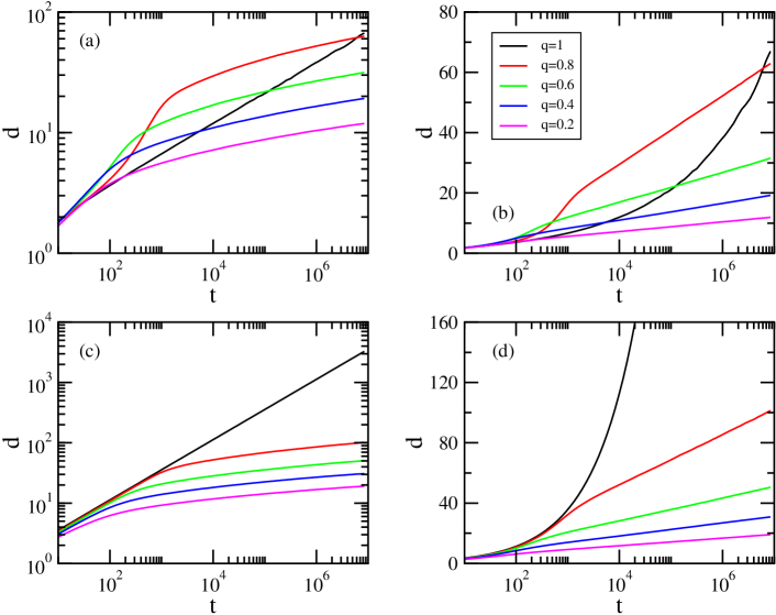
The data shown in Fig. 7a and 7b for the ring reveal a behavior that at first look seems odd. Indeed for $q=1$ one does not observe the free diffusion of particle, but instead the particles move sub-diffusively, with a mean displacement $d\sim t^{1/4}$. In order to understand this, let us recall that in the definition of the ABC model, see Section II, exchanges between particles of the same type are not assumed. In fact, for all aspects discussed in previous papers as well as for all the time-dependent quantities studied in our work, with the exception of the mean displacement, it is completely irrelevant whether we allow exchanges of same particles or not. However, for individual trajectories this does matter, as without these exchanges particles get stuck behind others of the same type and can only move if a particle of a different type comes by and replaces the particle on the neighboring site. Indeed, when allowing for these additional exchanges, we do recover free diffusion for $q=1$ also in one dimension, and for $q<1$ a crossover between that early time behavior and a logarithmic regime is observed, see Fig. 7c and 7d.

In the two-dimensional system shown in Fig. 6 particles get rarely stuck as they can diffuse both in $x$- and $y$-direction. Consequently, we have for $q=1$ the expected square-root behavior of a random walk even in absence of exchanges between particles of the same species.

Figure 8: (Color online) Scaling of the equal-time correlation function for $q=0.8$ and different system sizes. Data ranging from $t=100000$ to $t=500000$ are included. (a) Rescaled data for a system with $600\times 100$ sites. The inset shows the unscaled data. (b) Comparison of the scaling functions for three different system sizes. The inset shows the scaling of the correlator for a ring with 600 sites and three different values of the swapping rate $q$. The values of the scaling exponent $b$ that achieve the best data collapse are gathered in Table 1. For the larger systems these data result from averaging over more than 1000 independent realizations, whereas for the one-dimensional system the ensemble average is performed over 16000 independent runs.

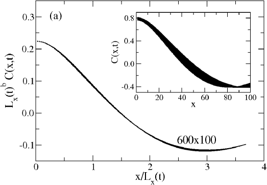
For systems governed by a time-dependent length scale $L_{x}(t)$ one expects from general considerations Bra93 that the single-time correlator $C({\bf r},t)$ exhibits a simple scaling behavior of the form Hen10

$$C({\bf r},t)=\left(L_{x}(t)\right)^{-b}f\left(\frac{\left|{\bf r}\right|}{L_{x}(t)}\right)$$ (8)

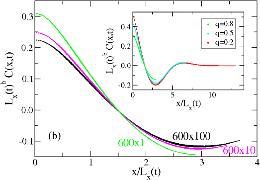
for sufficiently large times $t\gg t_{micro}$, where $t_{micro}$ is a microscopic reference time such that $L_{x}(t_{micro})$ is larger than any microscopic length scale. In the present case $t_{micro}$ has to be larger than the typical time needed for the formation of ordered stripes. As shown in Fig. 8a, once the logarithmic growth regime has been fully accessed, dynamical scaling prevails and a data collapse is achieved when assuming the scaling (8). The values of the scaling exponent $b$ are gathered in Table 1 for three different vertical extents and three different values of the swapping rate $q$. Inspection of the table reveals a weak dependence on the number of lines in the system. In addition, the value of $b$ changes with $q$. A similar dependence is also seen for the scaling function itself, see the inset in Fig. 8b. It follows that for the $ABC$ model scaling functions and scaling exponents depend on system parameters. This is similar to what is seen in other systems with logarithmic growth Par10 ; Cor11 ; Cor12 ; Par12 ; Cor13 .

Finally, we note from Fig. 8b that the scaling functions for different extents in vertical direction are not identical for the finite times accessed in our simulations. This can be viewed as a ’finite-size’ effect, and the dependence of the scaling function (and, of course, of $L_{x}(t)$) on the vertical direction will vanish in the large volume limit and long time limit.

	$600\times 1$	$600\times 10$	$600\times 100$
$q=0.2$	$-0.07(1)$	$-0.12(1)$	$-0.12(2)$
$q=0.5$	$-0.11(1)$	$-0.15(1)$	$-0.21(2)$
$q=0.8$	$-0.16(1)$	$-0.22(1)$	$-0.25(2)$

Table 1: Values of the scaling exponent $b$ for three different systems and three different values of the swapping rate $q$.

IV Two-times quantities

Two-times quantities are used in many studies in order to elucidate relaxation processes and aging phenomena far from stationarity Hen10 . As the discussion of the equal-time correlation function has established the presence of dynamical scaling in our system, we expect the following scaling Hen10 for the two-times autocorrelation function $C(t,s)$, see Eq. (4):

$$C(t,s)=\left(L_{x}(s)\right)^{-b}F\left(\frac{L_{x}(t)}{L_{x}(s)}\right)$$ (9)

where the exponent $b$ should be the same as for the equal-time correlator (8). This scaling form assumes that $L_{x}(t)$, $L_{x}(s)\gg L_{x}(t_{micro})$ as well as $L_{x}(t)-L_{x}(s)\gg L_{x}(t_{micro})$. This last condition can be difficult to fulfill for a system with logarithmic growth, and sizeable finite-time corrections could spoil the expected scaling.

Figure 9: (Color online) Scaling of the two-times autocorrelation function $C(t,s)$ for a system composed of $600\times 10$ spins, with (a) $q=0.2$, (b) $q=0.5$, and (c) $q=0.8$. The insets show the autocorrelation as function of the time difference $t-s$ and reveal the aging properties of that quantity. The waiting times decrease from top to bottom. In all cases a good data collapse is achieved for the larger waiting times $s$ when assuming the scaling form (9), with $b$ given in Table 1. These data result from averaging over 8000 runs.

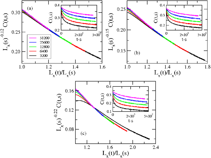
Fig. 9 explores the scaling (9) for a system with $600\times 10$ sites and three different swapping rates $q$. These three panels are also representatives for other system sizes and other values of $q$. Besides large waiting times $s$ for which we clearly are in the logarithmic growth regime, we also use rather short ones where in some cases the intermediate regime has not yet been left. We first remark that in all studied cases dynamical scaling (9) indeed prevails for the larger waiting times and $L_{x}(t)/L_{x}(s)$ not too close to 1. This is indeed achieved with the exponents listed in Table 1. On the other hand, finite-time corrections, which become less important for increasing $s$, are readily identified in the vicinity of $L_{x}(t)/L_{x}(s)\approx 1$. For the case $q=0.8$ shown in panel (c) the shortest waiting time $s=3600$ is obviously not yet in the scaling regime. Doing the same analysis for larger systems, say ones composed of $600\times 100$ sites, we have a data collapse only for waiting times for which the system left the crossover regime and entered the asymptotic logarithmic regime with ordered stripes.

Figure 10: (Color online) Time-dependent length when changing at the waiting time $s$ the swapping rate from $q_{i}=0.3$ to $q_{f}=0.2$ (dashed colored lines) and from $q_{i}=0.1$ to $q_{f}=0.2$ (full colored lines). The waiting times increase from left to right. The system sizes are (a) $600\times 1$, (b) $600\times 10$ and (c) $600\times 100$. The full black lines indicate the growing length for a system where $q$ is fixed at 0.3, 0.2, or 0.1 (from top to bottom). These data result from averaging over at least 1600 independent runs.

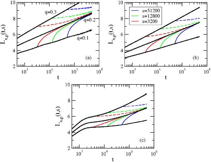
Whereas the two-times correlation function contains information on the time evolution of a system by comparing configurations at different times since its initial preparation, a two-times response function provides insights in how a system that still evolves reacts to a perturbation. A variety of protocols can be designed in order to probe the response of a system to a change of system parameters. As already discussed in Section II, we consider in the following sudden changes in the biased exchange rate $q$ and monitor how the perturbed system relaxes to the same state as that reached by a control system that evolves all the time at that final value of $q$.

Fig. 10 compares the length after the perturbation, $L_{x,p}(t,s)$, with that of the unperturbed system for two cases: (1) $q_{i}=0.3$ and $q_{f}=0.2$ (dashed lines) and (2) $q_{i}=0.1$ and $q_{f}=0.2$ (full lines). For systems with $600\times 1$ and $600\times 10$ sites the perturbations happen after the formation of the stripes. On the other hand, for the system with $600\times 100$ sites shown in panel (c) the perturbations take place close to the end of the intermediate regime but before the logarithmic growth is fully established. Qualitatively the responses for all three system sizes are very similar, though. In all cases the perturbed length tends to the corresponding length of the control system. This approach is rather fast for an increase of $q$ (in the present case from 0.1 to 0.2), but takes much longer for a decrease of $q$. When increasing $q$ the domains just after the change are too compact when compared to the domains that grow at the fixed value $q=0.2$. On the other hand, when considering the case where $q$ is decreased, the domains after the change are less dense than what should be the case for a $q=0.2$ system. Although $L_{x}(t=s)$ is larger for $q=0.3$ than that for $q=0.2$, $L_{x}(t)$ does not decrease after the quench, see the dashed lines in Fig. 10 that remain almost flat. Once the domains are formed, their size can not be reduced in a sizeable manner; the domain growth will be slowed down until the time $t_{0}$ when $L_{x}(t=t_{0})$ for the system evolving at the fixed rate $q=0.2$ is comparable to $L_{x}(t=s)$ for the $q=0.3$ system.

Figure 11: (Color online) Response function $M(t,s)$ for a system composed of $600\times 10$ particles after the diffusion bias has been changed from $q_{i}=0.3$ to $q_{f}=0.2$ at time $s$. The waiting times $s$ decrease from top to bottom. The inset shows a reasonable scaling $M(t,s)=\left(L_{x}(s)\right)^{-a}F_{M}\left(\frac{L_{x}(t)}{L_{x}(s)}\right)$ for the three largest waiting times with a scaling exponent $a=-1.48$.

In principle, the two-times response of a system to an infinitesimal instantaneous perturbation should display a scaling behavior similar to that of the two-times correlation function, see Eq. (9). In our case, however, the perturbation, i.e. the change in $q$, is a large one, with $\left|q_{f}-q_{i}\right|=0.1$. One should also note that a scaling behavior can not be expected when the perturbation takes place in a regime where $L_{x}(t)$ displays a crossover between different types of behaviors. Inspection of Fig. 10c, for example, reveals for the change from $q_{i}=0.1$ to $q_{f}=0.2$ a rather different behavior of $L_{x,p}(t,s)$ for $s=3600$ than for $s=51200$ (see full lines), and dynamical scaling can not be realized.

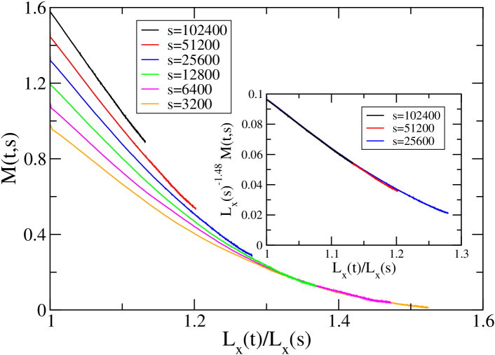
For an increase of $q$ we were unable to achieve a data collapse using as scaling variable $L_{x}(t)/L_{x}(s)$. This is different from when $q$ is decreased, however, as dynamical scaling can be identified in this case. Fig. 11 discusses as an example the change of $q$ from 0.3 to 0.2 for a system composed of $600\times 10$ sites. The difference $M(t,s)$ between the perturbed length $L_{x,p}(t,s)$ and the length $L_{x}(t)$ of the control system evolving with $q=0.2$, see Eq. (5), provides a quantity that displays aging as it does not merely depend on the time difference $t-s$. $M(t,s)$ goes to zero for long times when the ordered stripes of the perturbed system get similar to those of the unperturbed system. Inspection of Fig. 11 reveals the emergence of two different regimes: a regime where $M(t,s)$ is small (i.e. the perturbed length is close to the unperturbed one) and only depends on $L_{x}(t)/L_{x}(s)$, and a regime close to $L_{x}(t)/L_{x}(s)\approx 1$ where $M(t,s)$ is large and shifts to higher values for increasing waiting times $s$. In that regime a good scaling can be achieved when assuming that

$$M(t,s)=\left(L_{x}(s)\right)^{-a}F_{M}\left(\frac{L_{x}(t)}{L_{x}(s)}\right)~{},$$ (10)

see the inset in Fig. 11. We remark that immediately after the change of the value of $q$ the differences between the domains in the perturbed and in the control systems strongly depend on when the change took place, which gives raise to an increase of $M(t,s)$ with the waiting time $s$. However, once the ordered domains in the perturbed system have undergone major changes, they become similar to those that are formed in the control system, which results in a weaker dependence on $L_{x}(s)$.

V Conclusion

Phase-ordering kinetics in systems with algebraic domain growth, especially in cases where the domain coarsening is curvature driven, is rather well understood. Still open problems are encountered in disordered systems where after a transient algebraic-like growth regime a non-algebraic, logarithmic domain growth prevails for long times.

In this paper we discussed some aspects of domain coarsening in systems of a different type that are also characterized by logarithmic growth, namely in systems dominated by dynamical constraints. The best known representative of this class is the $ABC$ model Eva98a ; Eva98b where in a particular direction, say the horizontal direction, particles of three different types are exchanged asymmetrically. This leads to the formation of ordered domains which in a two-dimensional system take the form of stripes oriented perpendicularly to the direction of biased exchanges Kaf00 . In the asymptotic long-time regime, these domains coarsen and their size increases logarithmically with time.

Our emphasis was on the ordering process and the related aging phenomena. Studying a time-dependent length derived from the single-time spatial correlator, we identified different regimes that we discussed as a function of the vertical extent of the system and of the bias in the particle exchanges. Whereas in the logarithmic growth regime dynamical scaling prevails, as demonstrated by the data collapse of the single-time correlator as well as of the two-times autocorrelation (and also, to some extent, of the two-times response function), complicated crossover phenomena are observed during the formation of the well ordered stripes, especially in vertically extended systems where an intermediate phase is observed that is dominated by the vertical growth of the domains.

The attentive reader will have noticed that in the discussion of our results we never brought up the fact that for the one-dimensional system with even coverage for all three species the steady state is an equilibrium steady state, whereas in the two-dimensional version of the model detailed balance is always violated and the steady state is a non-equilibrium steady state. In fact, the equilibrium or non-equilibrium nature of the steady state does not seem to be relevant for the dynamical, far-from-stationarity regime probed in our study. While it seems reasonable that a system in the stages of domain formation and subsequent domain coarsening does not know anything about the character of the steady state emerging in the long time limit (see Oli93 ; Dro99 ; And06 for another example where the dynamic properties during relaxation do not depend on the equilibrium or non-equilibrium nature of the stationary state), there do exist well known examples (many-particle systems without detailed balance Hen07 , driven Ising systems Cor96 ; God11 ; God14 , driven striped structures Eva00 ) where for cases with a non-equilibrium steady state dynamic properties during the relaxation process are different from those encountered in the corresponding systems with an equilibrium steady state. Additional studies will be needed in the future in order to fully comprehend these differences.