Segregation of a Keplerian disc and sub-Keplerian halo from a Transonic flow around a Black Hole by Viscosity and Cooling processes

Abstract

A black hole accretion is necessarily transonic. In presence of sufficiently high viscosity and cooling effects, a low-angular momentum transonic flow can become a standard Keplerian disc except close to the where hole where it must pass through the inner sonic point. However, if the viscosity is not high everywhere and cooling is not efficient everywhere, the flow cannot completely become a Keplerian disc. In this paper, we show results of rigorous numerical simulations of a transonic flow having vertically varying viscosity parameter (being highest on the equatorial plane) and optical depth dependent cooling processes to show that the flow indeed segregates into two distinct components as it approaches a black hole. The component on the equatorial plane has properties of a standard Keplerian disc, though the flow is not truncated at the innermost stable circular orbit. This component extends till the horizon as a sub-Keplerian flow. This standard disc is found to be surrounded by a hot, low angular momentum component forming a centrifugal barrier dominated oscillating shock wave, consistent with the Chakrabarti-Titarchuk two component advective flow configuration.

1 Introduction

It is well known that a standard Keplerian disc (Shakura & Sunyaev, 1973, hereafter SS73; Novikov & Thorne, 1973) is not capable of explaining the entire X-ray and Gamma-ray spectrum characterizing an accreting black hole candidate. This is because SS73 disc emits a multicolour black body spectrum whereas a general observed spectrum contains an additional power-law component (e.g., Sunyaev & Truemper, 1979). Though there are several ad hoc models to explain power-law component (generally considered to arise out of Comptonization of soft photons by a hot electron cloud), Chakrabarti & Titarchuk (1995, hereafter CT95) explained the spectra using a truly global solution in which a sub-Keplerian (low-angular momentum) flow which produces a centrifugal barrier close to a black hole, and surrounds an SS73 disc (corrected at the inner edge), plays a major role. This so-called Two Component Advective Flow (TCAF) solution was taken straight out of theoretical study of the behaviour of topology of viscous flows around black holes (Chakrabarti, 1990, 1996). In a major breakthrough in understanding properties of a viscous transonic flow, it was pointed out (Chakrabarti 1990, 1996) that flows with super-critical viscosity parameter ($\alpha>\alpha_{crit}$) everywhere can only form a Keplerian disc. In CT95, precisely this property of the flow was used. One component with a $\alpha>\alpha_{crit}$ is a cooler, Keplerian disc on the equatorial plane, accreting in a viscous time scale. The second component is a low angular momentum flow with sub-critical ($\alpha<\alpha_{crit}$) viscosity parameter which forms a centrifugal pressure supported standing or oscillating shock and is accreting in almost a free-fall time scale. Later, many workers including Smith et al. (2001a), Smith et al. (2001b), Miller et al. (2001), Soria et al. (2009, 2011), Dutta & Chakrabarti (2010), Cambier & Smith (2013) found evidences of two components in many of the black hole candidates which motivated us to investigate into this configuration further.

Since TCAF claims to be the only theoretical solution which can describe the whole system, including hydrodynamic (disc plus outflows), spectral and temporal properties, its origin and stability are to be established by rigorous means. In a series of papers (Giri et al. 2010, hereafter Paper I; Giri & Chakrabarti, 2012, hereafter Paper II; Giri & Chakrabarti, 2013, hereafter III), it was shown how a viscous flow may produce a Keplerian disc on the equatorial plane if viscosity parameter is super-critical. Away from the equatorial plane, where viscosity parameter could be smaller, angular momentum distribution remains sub-Keplerian. A toy model was tried out in Paper III, where the entire flow was treated with a power-law cooling (not to be confused with the power-law spectrum produced due to Comptonization as mentioned earlier.) so that denser Keplerian disc could cool down faster while lighter sub-Keplerian halo remains hot and produces the CENtrifugal pressure dominated BOundary Layer or CENBOL, exactly as envisaged in CT95. However, a standard SS73 disc not only has a Keplerian distribution, it also emits a black body spectrum at a local temperature. So it needs to cool faster to emit such a radiation. In the present paper, we concentrate our attention to establish TCAF solution with hydrodynamic and radiative properties exactly as envisaged originally. We use the same time dependent hydrodynamic code as in Paper III, but instead of using a power-law cooling process (as a proxy to Comptonization which is stronger than the normal bremmstrahlung cooling) throughout, we use cooling processes which depend on optical depths at a given point. This process is expected to produce an SS73 type disc where optical depth is high and leave the lower optical depth region radiatively inefficient as in a low-angular momentum transonic flow.

2 Basic Equations anid Cooling Laws

Basic equations governing a two-dimensional axisymmetric flow around a Schwarzschild black hole have been presented extensively in earlier papers (Papers I-III) and we describe them here very briefly. Cylindrical coordinate system $(r,\phi,z)$ is adopted with z-axis being rotation axis of the disc. We use mass of the black hole $M_{BH}$, the velocity of light $c$ and Schwarzschild radius $R_{g}=2GM_{BH}/c^{2}$ as units of mass, velocity and distance respectively. Viscosity prescription has been used in a similar way as in Paper III. However, unlike Paper III, we incorporate cooling law differently. In each time step of our simulation, we use two types of coolings depending on optical depth of matter at a given computational grid.

At the beginning of our simulation, we start with a power-law cooling (as before) having a cooling rate of

$$\Lambda_{br}=1.4\times 10^{-27}N^{2}(r,z)T^{\beta}(r,z){\rm~{}erg~{}cm^{-3}~{}s^{-1}},$$

where, $N(r,z)$ is the number density and $T(r,z)$ is temperature of the flow at a location $(r,z)$. This power-law cooling was used as a proxy for Comptonization which is stronger than bremsstrahlung. For $\beta=0.5$, this becomes the well known bremsstrahlung cooling. Gas temperature $T$ at any ($r,z)$ is obtained from density ($\rho$) and pressure ($p$) obtained from our simulation using the ideal gas law:

$$T={p\over\rho}{{\mu{m_{p}}}\over{k_{b}}},$$

where, $k_{b}$ is Boltzmann constant, $\mu=0.5$, for purely hydrogen gas. Initially (transient period of the simulation) to increase the cooling efficiency, we took cooling index to be $\beta=0.6$ (as in Molteni, Sponholz & Chakrabarti, 1996). This was done to initiate the cooling process. At each time step, we compute optical depth,

$$\tau=\int N(r,z)\sigma_{T}dz,$$

where $\sigma_{T}$ is the Thomson scattering cross-section, along vertical directions starting from upper grid boundary to the equatorial plane. As soon as a Keplerian disc starts forming near the equatorial plane, we find a sudden increase in $\tau$ and we define the height where $\tau$ changes abruptly to be the surface of the disc. This surface is dynamically detected by the code. In case of an optically thick, geometrically thin Keplerian disc, energy is assumed to be radiated from the surface in the form of a black body radiation, with a cooling rate of

$$\Lambda_{bb}=\sigma T^{4}(r,z){\rm~{}erg~{}cm^{-2}~{}s^{-1}},$$

where, $\sigma$ is Stefan-Boltzmann constant given by $\sigma=5.67\times 10^{-5}~{}{\rm erg~{}cm^{-2}~{}deg^{-4}~{}s^{-1}}$. In regions below the surface of the disc, a separate cooling is no longer necessary as the energy produced in this region in expense of gravitational energy of the flow, is either diffused as above or advected into another grid. It is to be noted that advection is important in this component only close to the inner edge, where optical depth is never high enough to emit as a black body. Advection is also important in the sub-Keplerian region. In these two cases, cooling remains as in $\Lambda_{br}$ (Eqn. 1).

3 Setup of the Problem

Setup of our simulation is the same as presented in Paper III. We repeat only some key points. As before, we assume that gravitational field of the black hole can be described by Paczyński & Wiita (1980) pseudo-Newtonian potential,

$$\phi(r,z)=-{GM_{BH}\over(R-R_{g})},$$

where, $R=\sqrt{r^{2}+z^{2}}$. We assume a polytropic equation of state for accreting (or, outflowing) matter, $P=K\rho^{\gamma}$, where, $P$ and $\rho$ are the isotropic pressure and matter density respectively, $\gamma$ is a constant throughout the flow and $K$ is related to specific entropy of the flow $s$ (which need not be constant). In all our simulations, where the flow expected to be relativistic, we take $\gamma=4/3$.

The computational box occupies one quadrant of r-z plane with $0\leq r\leq 200$ and $0\leq z\leq 200$. We use reflection boundary condition on equatorial plane and z-axis to obtain a solution in other quadrants. Incoming gas enters the box through outer boundary located at $r_{b}=200$. We have chosen density of incoming gas ${\rho}_{in}=2.5$ for convenience. We supply radial velocity $v_{r}$ and sound speed $a$ of flow at outer boundary grids parallel to z-axis (at $r=r_{b}$). We take boundary values of density from standard vertical equilibrium solution of a transonic flow (Chakrabarti, 1989). We inject matter at outer boundary placed along z-axis. In order to the mimic horizon of the black hole, we place an absorbing inner boundary at $R=2.5R_{g}$, inside which all the matter is completely absorbed. Initially, the grid was filled with a background matter (BGM) of density ${\rho}_{bg}=10^{-6}$ having a sound speed (or, temperature) same as that of the injected matter. Hence, injected matter has $10^{6}$ times larger pressure than that of the BGM. The BGM is placed to avoid non-physical singularities caused by ‘division by zero’. This matter is quickly washed out and replaced by injected matter within a dynamical time scale. Calculations were performed with $512\times 512$ cells, so that each grid has a size of $0.39$ in units of Schwarzschild radius. Free fall timescale from the outer boundary is about $0.43$s as computed from the sum of $dr/<v_{r}>$ over the entire radial grid, $<v_{r}>$ being averaged over $20$ vertical grids.

All simulations have been carried out assuming a stellar mass black hole $(M_{BH}=10{M_{\odot}})$. We carry out simulations for several hundreds of dynamical time-scales. In reality, our simulation time corresponds to a few seconds in physical units. Conversion factor of our time unit to physical unit is $2GM_{BH}/c^{3}$, and thus physical time for which the program was run would scale with the mass of the black hole.

4 Simulation Results

We numerically solved system of equations discussed in Paper III and above, using a grid based finite difference method which is called Total Variation Diminishing (TVD) technique to deal with laboratory fluid dynamics (Harten, 1983) and was further developed by Ryu et al. (1995 & 1997) to study non-viscous astrophysical flows without cooling. We assume accretion flow to be in vertical equilibrium at the outer boundary so that we can inject matter according to theoretical transonic solution (Chakrabarti, 1989). The injection rate of momentum density is kept uniform throughout injected height at the outer boundary. Simulation is run till $t=95$ s, which is more than two hundred times the dynamical time. Thus, solutions presented by us are obtained long after the transient phase is over in about a second. We have run several cases. In Table 1, we show parameters used for the simulations at a glance. The case IDs are given in the first column. Columns 2 and 3 show specific energy ($\cal E$, energy per unit mass) and specific angular momentum ($\lambda$) of injected flow at outer boundary. The energy and the angular momentum are measured in the unit of $c^{2}$ and $r_{g}c$, respectively. In column 4, we present the injection rate of matter ($\dot{M}$) at the outer boundary. It is measured in the units of mass Eddington rate ($1.44\times 10^{17}M_{BH}$ gm/s). Finally, in column 5, we put values of viscous parameter, a dimensionless number $\alpha$. Results of our simulation are discussed below.

Case ID	${\cal E}$	$\lambda$	$\dot{M}$	$\alpha$
C1	$0.001$	$1.70$	$2.0$	$0.012$
C2	$0.001$	$1.70$	$1.5$	$0.012$
C3	$0.001$	$1.70$	$1.0$	$0.012$
C4	$0.001$	$1.70$	$0.5$	$0.012$
C5	$0.001$	$1.95$	$2.0$	$0.012$

Table 1: Parameters used for the simulations at a glance

In Fig. 1, we compare simulated specific angular momentum distributions throughout $r-z$ plane and corresponding Keplerian distribution for the case C1. This is a typical input for a transonic flow which we wish to convert to a Keplerian disc. In Fig. 1a, the result obtained from our simulation is shown.

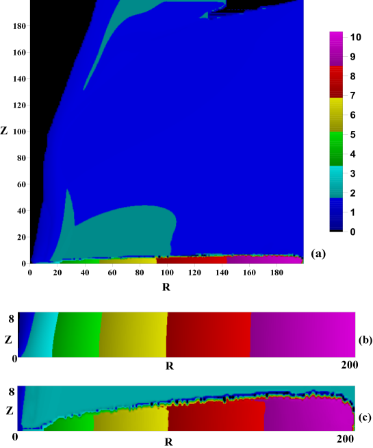
Figure 1: (a) Specific angular momentum distribution at $r-z$ plane in our simulation (Top panel) for C1. To compare with analytical results, region close to the equatorial plane is zoomed in to show (b) distribution in our simulated result and (c) Keplerian distribution.

In order to focus on our simulated Keplerian disc, in Fig. 1b, we zoom regions close to the equatorial plane while the same is shown in Fig. 1c for theoretical Keplerian distribution. Distributions in Fig. 1 (a-c) are plotted in linear scale. Different colours (online version) correspond to different specific angular momentum as marked in scale on right. It is to be noted that the outer front of Keplerian disc moves very slowly as compared to the inflow velocity of sub-Keplerian matter. In the frame of sub-Keplerian matter, the Keplerian disc behaves as an obstacle. This causes formation of an wake at the tip of the outer edge of simulated Keplerian flow. In a real situation, Keplerian disc will be extended till the outer boundary and Keplerian matter would be injected in those grids instead of a transonic flow. Our explicit procedure given here only demonstrates how a Keplerian disc forms in the first place, not by removal, but by redistribution of injected angular momentum.

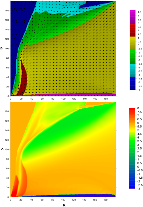
Figure 2: (a) Density and velocity distributions and (b) Temperature distribution with logarithmic scale at $r-z$ plane for C1. Densities in normalized units are plotted in logarithmic scale as in the scale on the right. Temperature in KeV units are plotted in logarithmic scale as in the scale on the right. A two component flow is clearly visible.

Fig. 2a shows velocity and density distributions of the flow and Fig. 2b temperature distributions in keV as per colour scale on right. Density distribution is plotted in logarithmic scale. The most prominent features are the formation of two component advective flow (TCAF). Both the Figures are for the case C1. Because of higher viscosity, the flow has a Keplerian distribution near the equatorial region. A Keplerian disc is formed out of sub-Keplerian matter by redistributing angular momentum. Simulation generated Keplerian disc is automatically truncated at $r\sim 15$ and a CENBOL is produced in between the Keplerian disk and the horizon. The region with Keplerian distribution becomes cooler and denser as matter settles on the equatorial plane. Comparatively low density, sub-Keplerian and hotter matter stays away from the equatorial plane. Liu et al. (2007) and Taam et al. (2008) investigated condensation of matter from a corona to a cool, optically thick inner disc. They focused on a simple theoretical model with Compton cooling which leads to condensation process and maintains a cool inner disc. In their simulations, both components were Keplerian. On the contrary, in our simulation, we inject sub-Keplerian flow with radial and vertical velocity distributions at the time of injection at outer boundary. We allow the matter to advect towards black hole as a transonic flow. With addition of viscosity, the distribution becomes close to Keplerian only close to equatorial plane. But, we required to add radiative cooling also to ensure that this Keplerian flow indeed radiates like a standard Keplerian disc. In our case, the two components rotate with two different rotational velocities and are therefore different from simulations by other groups. The boundary between these components is very thin and the Keplerian disc is not at all disrupted by Kelvin-Helmholz or other instability probably because of very high density in the Keplerian component.

Figure 3: Changes in (a) accretion rate ($\dot{M}_{disc}$) and (b) surface temperature of simulated Keplerian disc ($T_{disc}(r)$) with change of injected accretion rate parameter $\dot{M}$ at $t=95$ s. Here, $T_{disc}(r)$ is in keV unit, ($\dot{M}_{disc}$) is in Eddington rate unit and radius is in the Schwarzschild unit. For both the Figures, from top to bottom, the curves are for C1, C2, C3 & C4 respectively. For details, see the text.

In the next step, we study how the surface temperature distribution ($T_{disc}(r)$) and Keplerian disc accretion rate $\dot{M}_{disc}$ vary with injected accretion rate $\dot{M}$. One important point to note in these cases is that unlike SS73 disc model where $\dot{M}_{disc}$ is assumed to be constant at all radius for a given case, $\dot{M}_{disc}$ here appears to become radial distance dependent i.e., $\dot{M}_{disc}\equiv\dot{M}_{disc}(r)$. Therefore, we first calculate $\dot{M}_{disc}(r)$ i.e., the accretion rate of our simulated Keplerian disc in radial direction. At the radial distance $r$, the disc rate is obtained by $\sum(v_{r}\rho)2\pi rdz$, where, $v_{r}$ is the radial velocity and $\rho$ is the mass density of the flow at $r$. For each $r$, the $\sum$ is taken along $z$ direction over all the grid points from equatorial plane (i.e., $z=0$) to disc the surface. $T_{disc}(r)$ is easier to compute as it is the temperature of the grid point corresponding to disc surface. In Fig. 3, we compare radial variation of the accretion rate ($\dot{M}_{disc}(r)$) and surface temperatures ($T_{disc}(r)$) of our simulated Keplerian disc for different injected accretion rates ($\dot{M}$). We have taken four cases, i.e. C1, C2, C3 & C4 for this purpose. To make a comparison meaningful, all runs were carried out up to the same time, i.e, $95$s. Values of $\dot{M}$ for which curves have been drawn are (from bottom to top in Fig. 3): $0.5,\ 1.0,\ 1.5,\ 2.0$ respectively. It is known that local surface temperature of an SS73 disc is given by,

$$T(r)\approx 5.48\times 10^{7}(M_{BH})^{-1/4}(\dot{M}_{disc})^{1/4}(2r)^{-3/4}\left[1-\sqrt{\frac{3}{r}}\right]^{1/4}\mathrm{~{}K},$$

where the disc accretion rate $\dot{M}_{disc}$ is in units of Eddington rate. In Eqn. 7, it is evident that the surface temperature increases with Keplerian accretion rate $\dot{M_{disc}}$. For different runs, we vary injected accretion rates $\dot{M}$ and we see that the Keplerian accretion rate $\dot{M}_{disc}$ in simulated Keplerian disc will also vary in the same way. We see evidence of this in Fig. 3a. Surface temperature varies with our injected $\dot{M}$ and with $\dot{M}_{disc}$ which also adjusts itself with the variation of $\dot{M}$. Surface temperature which is obtained from our simulated Keplerian disc behaves like a standard SS73 disc, with some quasi-periodic ripples on them. Note that the accretion rate of the SS73-like component is not strictly constant, contrary to what is presently believed. :This has important implications in disc model fitting of observed data as was already pointed out in Dutta & Chakrabarti (2008). The ripples are important and depend on viscosity parameters. This will be discussed elsewhere.

Figure 4: Comparison of the disc rate $\dot{M}_{disc}$ and halo rate $\dot{M}_{halo}$ along radial direction in our simulation for C3 case. Here, accretion rate is in units of Eddington rate and the distance is in units of Schwarzschild radius.

We have shown disc accretion rate, i.e., $\dot{M}_{disc}$, for various model runs in Fig. 3. We do the same type of computation for simulated sub-Keplerian hot flow. This is the so-called ‘halo’ rate in CT95 ($\dot{M}_{halo}$). The formula for calculating radial variation of halo rate is the same as in disc rate, but, the $\sum$ is taken along $z$ direction from the disc surface to the top grid. It is to be noted that in our simulation, there is no distinguishing boundary between accreting and outflowing matter. Also, some part of matter which start as outflow from the region close to the black hole, fall back and become part of accreting halo. Therefore, it is difficult to compute halo accretion rate exactly. However, to draw a meaningful comparison, we compute $\dot{M}_{halo}$ for the case C3 and in Fig. 4, we compare $\dot{M}_{disc}$ and $\dot{M}_{halo}$ for the same case. It is evident that average disc rate varies around $0.15$ while that of halo rate is $0.7$. It is understandable that the rest of the injected matter moves away at $\dot{M}_{out}$ from the system as an outflow.

Figure 5: Variation of shock location with time (in seconds) when angular momentum is increased: (a) $\lambda=1.7$ (C1), (b) $1.95$ (C5).

Figure 6: Temporal variations of luminosity for both hot sub-Keplerian flow and Keplerian disc are shown when angular momentum is increased: (a) $\lambda=1.7$ (C1), (b) $1.95$ (C5). In each of the Figure, the top curve represents the hot flow while the bottom represents the Keplerian disc. Luminosity is in units of Eddington luminosity and time is in seconds. See text for details.

We now focus our attention to oscillation properties of shock locations by showing its dependence on flow parameters. This was pointed out to be the cause of quasi-periodic oscillations or QPOs (see, Molteni, Sponholz & Chakrabarti, 1996; Chakrabarti, Acharyya & Molteni, 2004 and Garain et al., 2014 for non-viscous flows). We choose $\lambda$ = $1.7$ and $1.95$ at the injected flow while keeping specific energy the same. In Figs. 5(a-b), we compare time variation of oscillations of shock locations. Mean shock location increases when $\lambda$ is increased from $1.7$ (C1) to $1.95$ (C5) due to enhancement in centrifugal pressure (Chakrabarti, 1989). We clearly see the presence of oscillations in both the cases. It is interesting to study time variation of luminosity of our simulated disc. We calculate luminosity of hot sub-Keplerian and as well as Keplerian components. There are Total luminosity of our simulated TCAF is the sum of these two luminosities. Radiation from hot, sub-Keplerian flow is dominated by bremsstrahlung in radiating layer throughout hot flow (including CENBOL) while disc luminosity is determined under the assumption of emission by a local black body and calculated as an integral over the Keplerian disc. In Figs. 6(a-b), we compare temporal variation of luminosities for both hot sub-Keplerian and Keplerian Components. Parameters are taken to be the same as before. In both the Figures, the top curve represents time variation of luminosity for power-law component (hot flow) while the bottom curve shows the same for black body component, i.e., the Keplerian disc. Because of very large volume of the sub-Keplerian component, its luminosity is higher than that of the SS73 disk by a large factor. This difference would be reduced with the increase in viscosity when more matter settles to the Keplerian component.

5 Discussions

The subject of accretion flow onto black holes has come a long way since the standard disc was proposed forty years ago. However, with the advent of precision observations, it became necessary to revise simplified solution obtained from a set of algebraic equations after addition of radial velocity, viscosity and radiative transfer and solving global differential equations. Almost twenty years ago, based on such a ‘generalized’ Bondi flow solution, (Chakrabarti, 1990, 1996), CT95 envisaged that spectral and temporal properties of galactic and extra-galactic black holes may be understood if we abandon the simplest assumption that all accretion flows must be necessarily Keplerian. This comes about due to the fact that the black hole accretion disc is always transonic (Chakrabarti, 1990) and thus it has to deviate from a (subsonic) Keplerian disc anyway. Furthermore, there could be return outflow which originates from (low-angular momentum) inner disc and winds of companions which can be accreted also. In the literature, simulations of viscosity parameter arising out of magnetorotational instability (MRI) did not yield a large value of $\alpha$ parameter beyond $0.01-0.1$. This is not enough to transport high value of angular momentum efficiently (Arlt & Rudiger, 2001; Masada & Sano, 2009). However these values are enough to transport low angular momentum matter and even to convert them to Keplerian discs. So we believe that CT95 scenario is reasonable. The belief is strengthened by the fact that most stellar mass black holes prefer to be in hard states where the SS73 disk plays a minor role.

Based on solutions of viscous transonic flows it was postulated that a transonic flow must split into a standard disc in regions of high viscosity parameter (near the equatorial plane), while regions lower $\alpha$ and inefficiently cooling matter would remain advective above and below the Keplerian disc. Though this configuration is widely used to fit satellite data, so far, it illuded confirmation through rigorous numerical simulations. In the present paper, we show, for the first time that the standard disc emitting black body on the equatorial plane can indeed survive even when it is sandwiched between fast moving (but slowly rotating) sub-Keplerian flows above and below. Not only that, the latter component, due to inefficient loss of angular momentum, ends up producing a centrifugal pressure dominated shock near the inner edge, evaporating Keplerian disc (making it truncated, so to speak) which behaves as the so-called Compton cloud, responsible for producing the power-law component of emitted spectrum by inverse Comptonization of intercepted soft photons emitted from the Keplerian disc. CENBOL is also believed to be responsible for producing jets and outflows. Its oscillation is responsible for low frequency QPOs. We believe that with this work, stability of TCAF solution is established and it can be safely used for fitting spectral and temporal properties.

While we assumed that the dynamical Keplerian disc surface emits black body radiation, we did not include effects of radiation pressure inside the disc itself and used only gas pressure. This is because accretion rate inside Keplerian component is highly sub-Eddington (less than $0.2{\dot{m}_{Ed}}$). In any case, since efficiency of emission for flows around a Schwarzschild black hole is only $6$ %, one requires tens of Eddington rates for radiation pressure to be dynamically important (e.g., slim disc model of Abramowicz et al., 1988, used fifty Eddington rate as illustration). This aspect will be investigated in future.

Since in our work, we did not explicitly use the cooling of hots flows by the Compton scattering, but used a power-law cooling as its proxy, it is interesting to compare these two cooling processes. This can be done using theoretical estimates.

Compton cooling rate for a thermal distribution of non-relativistic electrons (hot, sub-Keplerian flow in our case) of number density $n_{e}$ and temperature $T_{e}$ is (Rybicki & Lightman 1979)

$$C_{c}=\frac{4kT_{e}}{m_{e}c^{2}}cn_{e}\sigma_{T}U_{rad}\mathrm{~{}erg~{}cm^{-3}~{}s^{-1}},$$

where, $U_{rad}$ is the radiation energy density, $\sigma_{T}$ is the Thomson scattering cross-section, $c$ is the speed of light, $m_{e}$ is the mass of the electron and $k$ is the Boltzmann constant. We compute $U_{rad}$ from our simulation result, which is the black body radiation that is emitted from the disk surface and enters the sub-Keplerian flow. We can compute the energy loss ($C_{b}$) due to our assumed power-law cooling term (Eqn. 1). We take the ratio at different radial distances from the central black hole. We find that $C_{b}>C_{c}$ for $r\geq 100$; $C_{b}\sim C_{c}$ for $r\sim r_{shock}\leq 100$; and for $r<r_{shock}$, find $C_{b}<<C_{c}$. In other words, in the post-shock region Compton cooling is much more effective than the power-law cooling. Therefore, if we assume Compton cooling, we would expect lesser amount of hot flow in post-shock region compared to the amount obtained in our current simulation. Thus, hot flow rate may have been overestimated. Absence of the explicit Compton cooling is not going affect our conclusion of this paper, which is to say that in presence of viscosity and cooling, stable two-component advective flow is always possible.

It is to be noted that we have not explicitly included magnetic fields, though, we implicitly used viscosity parameters in the general range arising out of MRI. It is very difficult to ascertain what definite role magnetic fields play. However, it is clear that the presence of a dynamically strong poloidal magnetic field which threads both disc components would ensure efficient magneto-centrifugal transport of angular momentum (Blandford & Payne, 1982), enough to force them to act as a single component. However, if poloidal field is not dynamically important, two components will survive. What may happen is that the differential rotation would cause rapid amplification of toroidal component in dynamical time scale which may float out of discs due to buoyancy effects and collimate jets which originate from CENBOL surface (Chakrabarti & D’ Silva, 1994). This is outside the scope of the present paper, and will be investigated in future.

6 Acknowledgments

KG acknowledges support from National Science Council of the ROC through a post doctoral fellowship through grants NSC 101-2923-M-007 -001 -MY3 and 102-2112-M-007 -023 -MY3.

7 Bibliography

1. Abramowicz, M. A., Czerny, B., Lasota, J. P. & Szuszkiewicz, E., 1988, ApJ, 332, 646
2. Arlt, R. & Rüdiger, G., 2001, A & A, 374, 1035
3. Blandford, R.D. & Payne, D., 1982, MNRAS, 199, 883
4. Cambier, Hal J. & Smith, David M., 2013, ApJ, 767, 46
5. Chakrabarti, S.K. 1989, ApJ, 347, 365 (C89)
6. Chakrabarti S. K., 1990, MNRAS, 243, 610
7. Chakrabarti, S.K. & D’Silva, S. 1994, ApJ, 424, 138
8. Chakrabarti, S.K. & Titarchuk, L.G., 1995, ApJ, 455, 623 (CT95)
9. Chakrabarti, S. K., 1996, Phys. Rep., 266, 229 (C96)
10. Chakrabarti S. K., Acharyya K. A.& Molteni D., 2004, A & A, 421, 1
11. Dutta, B. G. & Chakrabarti, S. K., 2010, 404, 2136
12. Garain, S. K., Ghosh, H., & Chakrabarti, S. K., 2014, MNRAS, 437, 1329
13. Giri, K., Chakrabarti, S. K., Samanta, M., & Ryu, D. 2010, MNRAS 403,516
14. Giri, K. & Chakrabarti, S. K., 2012, MNRAS, 421, 666
15. Giri, K. & Chakrabarti, S. K., 2013, MNRAS, 430, 2836
16. Harten, A., 1983, J. Comp. Phys., 49, 357
17. Liu, B. F., Taam, R. E., Meyer, F., & Meyer-Hofmeister, E., 2007, ApJ, 671, 695
18. Masada, Y. & Sano, T. 2009, IAU Symposium No. 259, 121
19. Miller, J. M., Fox, D. W., Di Matteo, T., Wijnands, R., Belloni, T., Pooley, D., Kouveliotou, C., Lewin & W. H. G.,2001, ApJ, 546, 1055
20. Molteni, D., Sponholz, H. & Chakrabarti, S. K., 1996, ApJ, 457, 805
21. Novikov, I. D. and Thorne, K. S., 1973, in Black Holes, ed. B. S. De Witt and C. De Witt (New York: Gordon & Breach), 343
22. Paczyński, B. & Wiita, P. J., 1980, A & A, 88, 23
23. Rybicki, G. B. & Lightman, A. P., 1979, Radiative Processes in Astrophysics (New York: Wiley-Interscience)
24. Ryu, D., Brown, G. L., Ostriker, J. P. & Loeb, A., 1995, ApJ, 452, 364
25. Ryu, D., Chakrabarti, S. K. & Molteni, D., 1997, ApJ, 378, 388
26. Shakura, N. I. and Sunyaev, R. A. 1973, A & A, 24, 337 (SS73)
27. Smith, D. M., Heindl, W. A., Markwardt, C., & Swank, J. H., 2001b, ApJ, 554, L41
28. Smith, D. M., Heindl, W. A., & Swank, J. H., 2001a, AAS,33,1473
29. Soria, R., Risaliti, G., Elvis, M., Fabbiano, G., Bianchi, S., & Kuncic, Z, 2009, ApJ, 695, 1614
30. Soria, R., Broderick, J. W., Hao, J., Hannikainen, D.C., Mehdipour, M., Pottschmidt, K. & Zhang, S.N., 2011, MNRAS, 415, 410
31. Sunyaev R. A., Truemper J., 1979, Nat, 279, 506
32. Taam, R. E., Liu, B.F., Meyer, F., & Meyer-Hofmeister, E., 2008, ApJ, 688, 527