Critical exponents on Fortuin–Kasteleyn weighted planar maps

Abstract

In this paper we consider random planar maps weighted by the self-dual Fortuin–Kasteleyn model with parameter $q\in(0,4)$. Using a bijection due to Sheffield and a connection to planar Brownian motion in a cone we obtain rigorously the value of the critical exponent associated with the length of cluster interfaces, which is shown to be

$$\frac{4}{\pi}\arccos\left(\frac{\sqrt{2-\sqrt{q}}}{2}\right)=\frac{\kappa^{\prime}}{8}.$$

where $\kappa^{\prime}$ is the SLE parameter associated with this model. We also derive the exponent corresponding to the area enclosed by a loop which is shown to be 1 for all values of $q\in(0,4)$. Applying the KPZ formula we find that this value is consistent with the dimension of SLE curves and SLE duality.

Keywords: Random planar maps, self-dual Fortuin–Kasteleyn percolation, critical exponents, Liouville quantum gravity, KPZ formula, Schramm–Loewner Evolution, cone exponents for Brownian motion, SLE duality, isoperimetric relations, Sheffield’s bijection.

2010 MSC classification: 60K35, 60J67, 60D05

Figure 1: FK-weighted random map and loops for $q=0.5$ (left) and $q=2$ (corresponding to the Ising model, right). The shade of loops indicates their length (dark for short and light for long loops).

1 Introduction

Random surfaces have recently emerged as a subject of central importance in probability theory. On the one hand, they are connected to theoretical physics (in particular string theory) as they are basic building blocks for certain natural quantizations of gravity [34, 17, 28, 18]. On the other hand, at the mathematical level, they show a very rich and complex structure which is only beginning to be unravelled, thanks in particular to recent parallel developments in the study of conformally invariant random processes, Gaussian multiplicative chaos, and bijective techniques. We refer to [23] for a beautiful exposition of the general area with a focus on relatively recent mathematical developments.

This paper is concerned with the geometry of random planar maps, which can be thought of as canonical discretisations of the surface of interest. The particular distribution on planar maps which we consider was introduced in [36] and is roughly the following (the detailed definitions follow in Section 2.1). Let $q<4$ and let $n\geq 1$. The random map $M_{n}$ that we consider is decorated with a (random) subset $T_{n}$ of edges. The map $T_{n}$ induces a dual collection of edges $T_{n}^{\dagger}$ on the dual map of $M$ (see Figure 2). Let $\mathbf{m}$ be a planar map with $n$ edges, and $\mathbf{t}$ a given subset of edges of $\mathbf{m}$. Then the probability to pick a particular $(\mathbf{m},\mathbf{t})$ is, by definition, proportional to

$$\mathbb{P}(M_{n}=\mathbf{m},T_{n}=\mathbf{t})\propto\sqrt{q}^{\ell},$$ (1.1)

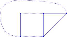
1.   2.

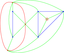
3.   4.

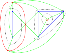
Figure 2: A map $m$ decorated with loops associated with a set of open edges $t$. Top left: the map is in blue, with solid open edges and dashed closed edges. Top right: Open clusters and corresponding open dual clusters in blue and red. Bottom left: every dual vertex is joined to its adjacent primal vertices by a green edge. This results in an augmented map $\bar{m}$ which is a triangulation. Bottom right: the primal and dual open clusters are separated by loops, which are drawn in black and are dashed. Each loop crosses every triangle once, and so can be identified with the set of triangles it crosses. See Section 2.1 for details.

where $\ell$ is the (total) number of loops in between both primal and dual vertex clusters in $\mathbf{t}$ which is equal to the combined number of cluster in $T_{n}$ and $T_{n}^{\dagger}$ minus $1$ (details in Section 2.1). Equivalently given the map $M_{n}=\mathbf{m}$, the collection of edges $T_{n}$ follows the distribution of the self-dual Fortuin–Kasteleyn model, which is in turn closely related to the critical $q$-state Potts model, see [3]. Accordingly, the map $M_{n}$ is chosen with probability proportional to the partition function of the Fortuin-Kasteleyn model on it.

One reason for this particular choice is the belief (see e.g. [20]) that after Riemann uniformisation, a large sample of such a map closely approximates a Liouville quantum gravity surface. This is the random metric obtained by considering the Riemannian metric tensor

$$e^{\gamma h(z)}|dz|^{2},$$ (1.2)

where $h(z)$ is an instance of the Gaussian free field. (We emphasise that a rigorous construction of the metric associated to (1.2) is still a major open problem.) The parameter $\gamma\in(0,2)$ is then believed to be related to the parameter $q$ of (1.1) by the relation

$$q=2+2\cos\left(\frac{8\pi}{\kappa^{\prime}}\right);\quad\gamma=\sqrt{\frac{16}{\kappa^{\prime}}}.$$ (1.3)

Note that when $q\in(0,4)$ we have that $\kappa^{\prime}\in(4,8)$ so that it is necessary to generate the Liouville quantum gravity with the associated dual parameter $\kappa=16/\kappa^{\prime}\in(0,4)$. This ensures that $\gamma=\sqrt{\kappa}\in(0,2)$, which is the nondegenerate phase for the associated mass measure and Brownian motions, see [21, 6, 7].

Observe that when $q=1$, the FK model reduces to ordinary bond percolation. Hence this corresponds to the case where $M$ is chosen according to the uniform probability distribution on planar maps with $n$ edges. This is a situation in which remarkably detailed information is known about the structure of the planar map. In particular, a landmark result due to Miermont [31] and Le Gall [29] is that, viewed as a metric space, and rescaling edge lengths to be $n^{-1/4}$, the random map converges to a multiple of a certain universal random metric space, known as the Brownian map. (In fact, the results of Miermont and Le Gall apply respectively to uniform quadrangulations with $n$ faces and to $p$-angulation for $p=3$ or $p$ even, whereas the convergence result concerning uniform planar maps with $n$ edges was established a bit later by Bettinelli, Jacob and Miermont [11]). Critical percolation on a related half-plane version of the maps has been analysed in a recent work of Angel and Curien [1], while information on the full plane percolation model was more recently obtained by Curien and Kortchemski [16]. Related works on loop models (sometimes rigorous, sometimes not) appear in [24, 14, 22, 10, 12, 13].

The goal of this paper is to obtain detailed geometric information about the clusters of the self-dual FK model in the general case $q\in(0,4)$. As we will see, our results are in agreement with nonrigorous predictions from the statistical physics community. In particular, after applying the KPZ transformation, they correspond to Beffara’s result about the dimension of SLE curves [4] and SLE duality.

1.1 Main results

Let $L_{n}$ denote a typical loop, that is, a loop chosen uniformly at random from the set of loops induced by $(M_{n},T_{n})$ which follow the law given by (1.1). Such a loop separates the map into an outside component which contains the root and an inside component which does not contain the root (precise definitions follow in Section 2.1). If the loop passes through the root, we leave $L_{n}$ undefined (this is a low probability event so the definition does not matter). Let $\textsf{Len}(L_{n})$ denote the number of triangles in the loop and let $\textsf{Area}(L_{n})$ denote the number of triangles inside it. Let

$$p_{0}=\frac{\pi}{4\arccos\left(\frac{\sqrt{2-\sqrt{q}}}{2}\right)}=\frac{\kappa^{\prime}}{8}$$ (1.4)

where $q$ and $\kappa^{\prime}$ are related as in (1.3).

Theorem 1.1.

We have that $\textsf{Len}(L_{n})\to\mathsf{L}$ and $\textsf{Area}(L_{n})\to\mathsf{A}$ in law. Further, the random variables $\mathsf{L}$ and $\mathsf{A}$ satisfy the following.

$$\mathbb{P}(\mathsf{L}>k)=k^{-1/p_{0}+o(1)},$$ (1.5)

and

$$\mathbb{P}(\mathsf{A}>k)=k^{-1+o(1)}.$$ (1.6)

Remark 1.2.

As we were finishing this paper, we learnt of the related work, completed independently and simultaneously, by Gwynne, Mao and Sun [26]. They obtain several scaling limit results, showing that various quantities associated with the FK clusters converge in the scaling limit to the analogous quantities derived from Liouville quantum gravity in [20]. Some of their results also overlap with the results above. In particular they obtain a stronger version of the length exponent (1.5) by showing that in addition that the tails are regularly varying. Though both papers rely on Sheffield’s bijection [36] and a connection to planar Brownian motion in a cone, it is interesting to note that the proof techniques are substantially different. The techniques in this paper are comparatively simple, relying principally on harmonic functions and appropriate martingale techniques.

Returning to Theorem 1.1, it is in fact not so hard to see that when rooted at a randomly chosen edge, the decorated maps $(M_{n},T_{n})$ themselves converge for the Benjamini–Schramm (local) topology. This is already implicit in the work of Sheffield [36] and properties of the infinite local limit $(M_{\infty},T_{\infty})$ have recently been analysed in a paper of Chen [15]. In particular a uniform exponential bound on the degree of the root is obtained. Together with earlier results of Gurel Gurevich and Nachmias [25], this implies for instance that random walk on $M_{\infty}$ is a.s. recurrent. From this it is actually not hard to see that $\textsf{Len}(L_{n})$ and $\textsf{Area}(L_{n})$ converge in law in Theorem 1.1. The major contributions in this paper are the other assertions in Theorem 1.1.

Our results can also be phrased for the loop $L^{*}$ going through the origin in this infinite map $M_{\infty}$. Since the root is uniformly chosen from all possible oriented edges, it is easy to see that this involves biasing by the length of a typical loop. Hence the exponents are slightly different. For instance, for the length $\textsf{Len}(L^{*})$ and $\textsf{Area}(L^{*})$ of $L^{*}$, we get

$$\mathbb{P}(\textsf{Len}(L^{*})>k)=k^{-1/p_{0}+1+o(1)},$$ (1.7)

For the area, it can be seen from our techniques that

$$\mathbb{P}(\textsf{Area}(L^{*})\geq k)=k^{-(1-p_{0})+o(1)},$$ (1.8)

(The authors of [26] have kindly indicated to us that (1.8), together with a regular variation statement, could probably also be deduced from their Corollary 5.3 with a few pages of work, using arguments similar to those already found in their paper).

While our techniques could also probably be used to compute other related exponents we have not pursued this, in order to keep the paper as simple as possible. We also remark that the techniques in the present paper can be used to study the looptree structure of typical cluster boundaries (in the sense of Curien and Kortchemski [16]).

Remark 1.3.

In the particular case of percolation on the uniform infinite random planar map (UIPM) $M_{\infty}$, i.e. for $q=1$, we note that our results give $p_{0}=3/4$, so that the typical boundary loop exponent is $1/p_{0}=4/3$. This is consistent with the more precise asymptotics derived by Curien and Kortchemski [16] for a related percolation interface. Essentially their problem is analogous to the biased loop case, for which the exponent is, as discussed above, $1/p_{0}-1=1/3$. This matches Theorem 1 in [16], see also Theorem 2 (ii) in [1] for the half-plane case. Likewise, the exponent for the area of $L^{*}$ (in the biased case) is $1-p_{0}=1/4$, which matches (i) in the same theorem of [1].

1.2 Cluster boundary, KPZ formula, bubbles and dimension of SLE

KPZ formula. We now discuss how our results verify the KPZ relation between critical exponents. We first recall the KPZ formula. For a fixed or random independent set $A$ with Euclidean scaling exponent $x$, its “quantum analogue” has a scaling exponent $\Delta$, where $x$ and $\Delta$ are related by the formula

$$x=\frac{\gamma^{2}}{4}\Delta^{2}+(1-\frac{\gamma^{2}}{4})\Delta.$$ (1.9)

See [21, 7, 35] for rigorous formulations of this formula at the continuous level. Concretely, this formula should be understood as follows. Suppose that a certain subset $A$ within a random map of size $N$ has a size $|A|\approx N^{1-\Delta}$. Then its Euclidean analogue within a box of area $N$ (and thus of side length $n=\sqrt{N}$) occupies a size $|A^{\prime}|\approx N^{1-x}=n^{1/2-x/2}.$ In particular, observe that the approximate (Euclidean) Hausdorff dimension of $A^{\prime}$ is then $2-2x$.

Cluster boundary.

The exponents in (1.5) and (1.6) suggest that for a large critical FK cluster on a random map, we have the following approximate relation between the area and the length:

$$\mathsf{L}=\mathsf{A}^{p_{0}+o(1)}.$$ (1.10)

The relation (1.10) suggests that the quantum scaling exponent $\Delta=1-p_{0}$. Applying the KPZ formula we see that the corresponding Euclidean exponent is $1/2-\kappa^{\prime}/16$. Thus the Euclidean dimension of the boundary is $1+\kappa^{\prime}/8$. The conjectured scaling limits of the boundary is a CLE${}_{\kappa^{\prime}}$ curve and hence this exponent matches the one obtained by Beffara [4].

Bubble boundary.

We now address a different sort of relation with its volume inside, which concerns large filled-in bubbles or envelopes in the terminology which we use in this paper (see Definition 2.2 and immediately above for a definition). In the scaling limit and after a conformal embedding, these are expected to converge to filled-in SLE loops and more precisely, quantum discs in the sense of [20]. At the local limit level, they should correspond to Boltzmann maps whose boundaries should form a looptree structure in the sense of Curien and Kortchemski [16]. We establish in Theorem 3.2, items iv and v that with high probability

$$|\partial\mathcal{B}|=|\mathcal{B}|^{1/2+o(1)}.$$ (1.11)

This suggests a quantum dimension of $\Delta=1/2$ and remarkably, this boundary bulk behaviour is independent of $q$ (or equivalently of $\gamma$) and therefore corresponds with the usual Euclidean isoperimetry in two dimensions. Applying the KPZ formula (1.9), we obtain a Euclidean scaling exponent

$$x=\frac{1}{2}-\frac{1}{\kappa^{\prime}}.$$

On the other hand, recall the Duplantier duality which states that the outer boundary of an SLE${}_{\kappa^{\prime}}$ curve is an SLE${}_{16/{\kappa^{\prime}}}$ = SLE_κ curve. This has been established in many senses in [32, 19, 37]. Hence the dimension of the outer boundary should be $1+\kappa/8=1+2/\kappa^{\prime}$ which is equal to $2(1-x)$. Thus KPZ is verified.

Acknowledgements We are grateful to a number of people for useful discussions: Omer Angel, Linxiao Chen, Nicolas Curien, Grégory Miermont, Jason Miller, Scott Sheffield, and Perla Sousi. We thank Ewain Gwynne, Cheng Mao and Xin Sun for useful comments on a preliminary draft, and for sharing and discussing their results in [26] with us. Part of this work was completed while visiting the Random Geometry programme at the Isaac Newton Institute. We wish to express our gratitude for the hospitality and the stimulating atmosphere.

2 Background and setup

2.1 The critical FK model

Recall that a planar map is a proper embedding of a (multi) graph with $n$ edges in the plane which is viewed up to orientation preserving homeomorphisms from the plane to itself. Let $\boldsymbol{m}_{n}$ be a map with $n$ edges and $\boldsymbol{t}_{n}$ be the subgraph induced by a subset of its edges and all of its vertices. We call the pair $(\boldsymbol{m}_{n},\boldsymbol{t}_{n})$ a submap decorated map. Let $\boldsymbol{m}_{n}^{\dagger}$ denote the dual map of $\boldsymbol{m}_{n}$. Recall that the vertices of the dual map correspond to the faces of $\boldsymbol{m}_{n}$ and two vertices in the dual map are adjacent if and only if their corresponding faces are adjacent to a common edge in the primal map. Every edge $e$ in the primal map corresponds to an edge $e^{\dagger}$ in the dual map which joins the vertices corresponding to the two faces adjacent to $e$. The dual map $\boldsymbol{t}_{n}^{\dagger}$ is the graph formed by the subset of edges $\{e^{\dagger}:e\notin\boldsymbol{t}_{n}\}$. We fix an oriented edge in the map $\boldsymbol{m}_{n}$ and define it to be the root edge.

Given a subgraph decorated map $(\boldsymbol{m}_{n},\boldsymbol{t}_{n})$, one can associate to it a set of loops which form the interface between the two clusters. To define it precisely, we consider a refinement of the map $\boldsymbol{m}_{n}$ which is formed by joining the dual vertices in every face of $\boldsymbol{m}_{n}$ with the primal vertices incident to that face. We call these edges refinement edges. Every edge in $\boldsymbol{m}_{n}$ corresponds to a quadrangle in its refinement formed by the union of the two triangles incident to its two sides. In fact the refinement of $\boldsymbol{m}_{n}$ is a quadrangulation and this construction defines a bijection between maps with $n$ edges and quadrangulations with $n$ faces.

There is an obvious one-one correspondence between the refinement edges and the oriented edges in a map. Every oriented edge comes with a head and a tail and a well defined triangle to its left. Simply match every oriented edge with the refinement edge of the triangle to its left which is incident to its tail. We call such an edge the refinement edge corresponding to the oriented edge.

Given a subgraph decorated map $(\boldsymbol{m}_{n},\boldsymbol{t}_{n})$ define the map $(\bar{\boldsymbol{m}}_{n},\bar{\boldsymbol{t}}_{n})$ to be formed by the union of $\boldsymbol{t}_{n},\boldsymbol{t}_{n}^{\dagger}$ and the refinement edges. The root edge of $(\bar{\boldsymbol{m}}_{n},\bar{\boldsymbol{t}}_{n})$ is the refinement edge corresponding to the root edge in $\boldsymbol{m}_{n}$ oriented towards the dual vertex. The root triangle is the triangle to the right of the root edge. It is easy to see that such a map is a triangulation: every face in the refinement of $\boldsymbol{m}_{n}$ is divided into two triangles either by a primal edge in $\boldsymbol{t}_{n}$ or a dual edge in $\boldsymbol{t}_{n}^{\dagger}$. Thus every triangle in $(\bar{\boldsymbol{m}}_{n},\bar{\boldsymbol{t}}_{n})$ is formed either by a primal edge and two refinement edges or by a dual edge and two refinement edges. For future reference, we call a triangle in $(\bar{\boldsymbol{m}}_{n},\bar{\boldsymbol{t}}_{n})$ with a primal edge to be a primal triangle and that with a dual edge to be a dual triangle (Figure 3).

Finally we can define the interface as a subgraph of the dual map of the triangulation $(\bar{\boldsymbol{m}}_{n},\bar{\boldsymbol{t}}_{n})$. Simply join together faces in the adjacent triangles which share a common refinement edge. Clearly, such the interface is “space filling” in the sense that every face in $(\bar{\boldsymbol{m}}_{n},\bar{\boldsymbol{t}}_{n})$ is traversed by an interface. Also it is fairly straightforward to see that an interface is a collection of simple cycles which we refer to as the loops corresponding to the configuration $(\boldsymbol{m}_{n},\boldsymbol{t}_{n})$. Also such loops always have primal vertices one its one side and dual vertices on its other side. Also every loop configuration corresponds to a unique configuration $\boldsymbol{t}_{n}$ and vice versa. Let $\ell(\boldsymbol{m}_{n},\boldsymbol{t}_{n})$ denote the number of loops corresponding to a configuration $(\boldsymbol{m}_{n},\boldsymbol{t}_{n})$. The critical FK model with parameter $q$ is a random configuration $(M_{n},T_{n})$ which follows the law

$$\mathbb{P}((M_{n},T_{n})=(\boldsymbol{m}_{n},\boldsymbol{t}_{n}))\propto\sqrt{q}^{\ell(\boldsymbol{m}_{n},\boldsymbol{t}_{n})}$$ (2.1)

The model makes sense for any $q\in[0,\infty)$ but we shall focus on $q\in[0,4)$. It is also easy to see that the law of $(M_{n},T_{n})$ remains unchanged if we re-root the map at an independently and uniformly chosen oriented edge (see, for example, [2] for an argument).

Let $c(t_{n})$ and $c(t_{n}^{\dagger})$ denote the number of vertex clusters of $t_{n}$ and $t_{n}^{\dagger}$. Recall that the loops form the interface between primal and dual vertex clusters. From this, it is clear that $\ell(\boldsymbol{m}_{n},\boldsymbol{t}_{n})=c(t_{n})+c(t_{n}^{\dagger})-1$. Let $v(G),e(G)$ denote the number of vertices and edges in a graph $G$. An application of Euler’s formula shows that

$$\mathbb{P}(\boldsymbol{m}_{n})=\frac{1}{Z}(\sqrt{q})^{-v(\boldsymbol{m}_{n})}\sum_{G\subset\boldsymbol{m}_{n}}\sqrt{q}^{e(G)}q^{c(G)}.$$ (2.2)

where $Z$ denotes the partition function. It is easy to conclude from this that the model is self dual and hence critical. Note that (2.2) corresponds to the Fortuin-Kasteleyn random cluster model which is in turn is equivalent to the $q$-state Potts model on maps with $n$ edges (see [3]).

2.2 Sheffield’s bijection

We briefly recall the Hamburger–Cheeseburger bijection due to Sheffield (see also related works by Mullin [33] and Bernardi [8, 9]).

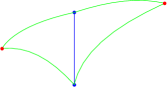
Figure 3: Refined or green edges split the map and its dual into primal and dual triangles. Each primal triangle sits opposite another primal triangle, resulting in a primal quadrangle as above.

Recall that the refinement edges split the map into triangles which can be of only two types: a primal triangle (meaning two green or refined edges and one primal edge) or a dual triangle (meaning two green or refined edges and one dual edge). For ease of reference primal triangles will be associated to hamburgers, and dual triangles to cheeseburgers. Now consider the primal edge in a primal triangle; the triangle opposite that edge is then obviously a primal triangle too. Hence it is better to think of the map as being split into quadrangles where one diagonal is primal or dual (see Figure 3).

We will reveal the map, triangle by triangle, by exploring it with a path which visits every triangle once (hence the word “space-filling”). We will keep track of the first time that the path enters a given quadrangle by saying that either a hamburger or a cheeseburger is produced, depending on whether the quadrangle is primal or dual. Later on, when the path comes back to the quadrangle for the second and last time, we will say that the burger has been eaten. We will use the letters $\textsf{h},\textsf{c}$ to indicate that a hamburger or cheeseburger has been produced and we will use the letters $\textsf{H},\textsf{C}$ to indicate that a burger has been eaten (or ordered and eaten immediately). So in this description we will have one letter for every triangle.

It remains to specify in what order are the triangles visited, or equivalently to describe the space-filling path. In the case where the decoration $\boldsymbol{t}_{n}$ consists of a single spanning tree (corresponding to $q=0$ as we will see later) the path is simply the contour path going around the tree. Hence in that case the map is entirely described by a sequence of $2n$ letters in the alphabet $\{\textsf{h},\textsf{c},\textsf{H},\textsf{C}\}$.

We now describe the situation when $\boldsymbol{t}_{n}$ is arbitrary, which is more delicate. The idea is that the space-filing path starts to go around the component of the root edge, i.e. explores the loop of the root edge, call it $L_{0}$. However, we also need to explore the rest of the map. To do this, consider the last time that $L_{0}$ is adjacent to some triangle in the complement of $L_{0}$, where by complement we mean the set of triangles which do not intersect $L_{0}$. (Typically, this time will be the time when we are about to close the loop $L_{0}$). At that time we continue the exploration as if we had flipped the diagonal of the corresponding quadrangle. This has the effect the exploration path now visits two loops. We can now iterate this procedure. A moment of thought shows that this results in a space-filling path which visit every quadrangle exactly twice, going around some virtual tree which is not needed for what follows. We record a flipping event by the symbol F. More precisely, we associate to the decorated map $(\boldsymbol{m}_{n},\boldsymbol{t}_{n})$ a list of $2n$ symbols $(X_{i})_{1\leq i\leq 2n}$ taking values in the alphabet $\Theta=\{\textsf{h},\textsf{c},\textsf{H},\textsf{C},\textsf{F}\}$. For each triangle visited by the space-filling exploration path we get a symbol in $\Theta$ defined as before if there was no flipping, and we use the symbol F the second time the path visit a flipped quadrangle.

It is not obvious but true that this list of symbols completely characterises the decorated map $(\boldsymbol{m}_{n},\boldsymbol{t}_{n})$. Moreover, observe that each loop corresponds to a symbol F (except the loop through the root).

2.3 Inventory accumulation

We now explain how to reverse the bijection. One can interpret an element in $\{\textsf{h},\textsf{c},\textsf{H},\textsf{C}\}^{2n}$ as a last-in, first-out inventory accumulation process in a burger factory with two types of products: hamburgers and cheeseburgers. Think of a sequence of events occurring per unit time in which either a burger is produced (either ham or cheese) or there is an order of a burger (either ham or cheese). The burgers are put in a single stack and every time there is an order of a certain type of burger, the freshest burger in the stack of the corresponding type is removed. The symbol h (resp. c) corresponds to a ham (resp. cheese) burger production and the symbol H (resp. C) corresponds to a ham (resp. cheese) burger order.

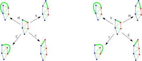
Figure 4: From symbols to map. The current position of the interface (or last discovered refined edge) is indicated with a bold line. Left: reading the word sequence from left to right or into the future. The map in the center is formed from the symbol sequence chc. Right: The corresponding operation when we go from right to left (or into the past). The map in the center now corresponds to the symbol sequence CHC.

Reversing the procedure when there is no F symbol is pretty obvious (see e.g. Figure 4). So we discuss the general case straight away. The inventory interpretation of the symbol F is the following: this corresponds to a customer demanding the freshest or the topmost burger in the stack irrespective of the type. In particular, whether an F symbol corresponds to a hamburger or a cheeseburger order depends on the topmost burger type at the time of the order. Thus overall, we can think of the inventory process as a sequence of symbols in $\Theta$ with the following reduction rules

• $\textsf{c}\textsf{C}=\textsf{c}\textsf{F}=\textsf{h}\textsf{H}=\textsf{h}\textsf{F}=\emptyset$,

• $\textsf{c}\textsf{H}=\textsf{H}\textsf{c}$ and $\textsf{h}\textsf{C}=\textsf{C}\textsf{h}$.

Given a sequence of symbols $X$, we denote by $\bar{X}$ the reduced word formed via the above reduction rule.

Given a sequence $X$ of symbols from $\Theta$, such that $\bar{X}=\emptyset$, we can construct a decorated map $(\boldsymbol{m}_{n},\boldsymbol{t}_{n})$ as follows. First convert all the F symbols to either a H or an C symbol depending on its order type. Then construct a spanning tree decorated map as is described above (Figure 4). The condition $\bar{X}=\emptyset$ ensures that we can do this. To obtain the loops, simply switch the type of every quadrangle which has one of the triangles corresponding to an F symbol. That is, if a quadrangle formed by primal triangles has one of its triangles coming from an F symbol, then replace the primal map edge in that quadrangle by the corresponding dual edge and vice versa. The interface is now divided into several loops and the number of loops is exactly one more than the number of F symbols.

Generating FK-weighted maps.

Fix $p\in[0,1/2)$. Let $X_{1},\ldots,X_{n}$ be i.i.d. with the following law

$$\mathbb{P}(\textsf{c})=\mathbb{P}(\textsf{h})=\frac{1}{4},\mathbb{P}(\textsf{C})=\mathbb{P}(\textsf{H})=\frac{1-p}{4},\mathbb{P}(\textsf{F})=\frac{p}{2}.$$ (2.3)

conditioned on $\overline{X_{1},\ldots,X_{n}}=\emptyset$.

Let $(\boldsymbol{m}_{n},\boldsymbol{t}_{n})$ be the random associated decorated map as above. Then observe that since $n$ hamburgers and cheeseburgers must be produced, and since $\#\textsf{H}+\#\textsf{C}=n-\#\textsf{F}$,

$$\mathbb{P}((\boldsymbol{m}_{n},\boldsymbol{t}_{n})) =\left(\frac{1}{4}\right)^{n}\left(\frac{1-p}{4}\right)^{\#\textsf{H}+\#\textsf{C}}\left(\frac{p}{2}\right)^{\#\textsf{F}}$$

$$\propto\left(\frac{2p}{1-p}\right)^{\#\textsf{F}}=\left(\frac{2p}{1-p}\right)^{\#\ell(\boldsymbol{m}_{n},\boldsymbol{t}_{n})-1}$$ (2.4)

Thus we see that $(\boldsymbol{m}_{n},\boldsymbol{t}_{n})$ is a realisation of the critical FK-weighted cluster random map model with $\sqrt{q}=2p/(1-p)$. Notice that $p\in[0,1/2)$ corresponds to $q=[0,4)$. From now on we fix the value of $p$ and $q$ in this regime. (Recall that $q=4$ is believed to be a critical value for many properties of the map).

2.4 Local limits and the geometry of loops

The following theorem due to Sheffield and made more precise later by Chen [36, 15] shows that the decorated map $(M_{n},T_{n})$ has a local limit as $n\to\infty$ in the local topology. Roughly two maps are close in the local topology if the finite maps near a large neighbourhood of the root are isomorphic as maps (see [5] for a precise definition).

Theorem 2.1 ([36, 15]).

Fix $p\in[0,1)$. We have

$$(M_{n},T_{n})\xrightarrow[n\to\infty]{(d)}(M,T)$$

in the local topology.

Furthermore, $(M,T)$ can be described by applying the obvious infinite version of Sheffield’s bijection to the bi-infinite i.i.d. sequence of symbols with law given by (2.3).

The idea behind the proof of Theorem 2.1 is the following. Let $X_{1},\ldots,X_{2n}$ be i.i.d. with law given by (2.3) conditioned on $\overline{X_{1}\ldots X_{2n}}=\emptyset$. It is shown in [36, 15] that the probability of $\overline{X_{1}\ldots X_{2n}}=\emptyset$ decays sub exponentially. Using Cramer’s rule one can deduce that locally the symbols around a uniformly selected symbol from $\{X_{i}\}_{1\leq i\leq n}$ converge to a bi-infinite i.i.d. sequence $\{X_{i}\}_{i\in\mathbb{Z}}$ in law. The proof is now completed by arguing that the correspondence between the finite maps and the symbols is continuous in the local topology.

Notice that uniformly selecting a symbol corresponds to selecting a uniform triangle in $(\bar{M}_{n},\bar{T}_{n})$ which in turn corresponds to a unique refinement edge which in turn corresponds to a unique oriented edge in $M_{n}$. Because of the above interpretation and the invariance under re-rooting, one can think of the triangle corresponding to $X_{0}$ as the root triangle in $(M,T)$.

One important thing that comes out of the proof is that every symbol in the i.i.d. sequence $\{X_{i}\}_{i\in\mathbb{Z}}$ has an almost sure unique match, meaning that every order is fulfilled and every burger is consumed with probability $1$. Let $\varphi(i)$ denote the match of the $i$th symbol. Notice that $\varphi:\mathbb{Z}\mapsto\mathbb{Z}$ defines an involution on the integers.

The goal of this section is to explain the connection between the geometry of the loops in the infinite map $(M,T)$ and the bi-infinite sequence $\{X_{i}\}_{i\in\mathbb{Z}}$ of symbols with law given by (2.3). For this, we describe an equivalent procedure to explore the map associated to a given sequence, triangle by triangle in the refined map $(\bar{M},\bar{T})$. (This is again defined in the same way as its finite counterpart: it is formed by the subgraph $T$, its dual $T^{\dagger}$ and the refinement edges.)

Loops, words and envelopes.

Recall that in the infinite (or whole-plane) decorated refined map $(\bar{M},\bar{T})$, each loop is encoded by a unique F symbol in the bi-infinite sequence of symbols $(X_{i})_{i\in\mathbb{Z}}$, and vice-versa. Suppose $X_{i}=\textsf{F}$ for some $i\in\mathbb{Z}$, and consider the word $W=X_{\varphi(i)}\ldots X_{i}$ and the reduced word $\mathcal{R}=\bar{W}$ (recall that $\varphi(i)$ is a.s. finite). Observe that $\mathcal{R}$ is necessarily of the form $\textsf{H}\ldots\textsf{H}$ or of the form $\textsf{C}\ldots\textsf{C}$ depending on whether $X_{\varphi(i)}=\textsf{c}$ or h, respectively. These symbols can appear any number of times, including zero if $\mathcal{R}=\emptyset$.

A moment of thought shows therefore that $W$ encodes a decorated submap of $(\bar{M},\bar{T})$ which we call the envelope of $X_{i}$, denoted by $\mathsf{e}(i)$ or sometimes $\mathsf{e}(X_{i})$ with an abuse of notation. Furthermore, this map is finite and simply connected. Assume without loss of generality that $\mathcal{R}$ contains only H symbols. Then the boundary of this map consists a connected arc of $|\mathcal{R}|$ primal edges and two green (refined) edges (see Figure 5). Note also that this map depends only on the symbols $(X_{j})_{\varphi(i)\leq j\leq i}$ (i.e., $W$ do not contain any F symbol whose match is outside $W$).

The complement of the triangles corresponding to a loop in $(\bar{M},\bar{T})$ consists of one infinite component and several finite components (there are several components if the loop forms fjords). Recall that the loop is a simple closed cycle in the dual of the refined map, hence it divides the plane (for any proper embedding) into an inside component and an outside component.

Definition 2.2.

Given a loop in the map $(\bar{M},\bar{T})$, the interior of the loop is the portion of the map corresponding to the triangles in the finite component of its complement and lying completely inside the loop. The rest of the triangles lie in the exterior of the loop. The length of the loop is the number of triangles corresponding to the vertices (in the dual refined map) in the loop, or equivalently, the number of triangles that the loop goes through. The area inside the loop is the number of triangles in its interior plus the length of the loop.

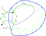
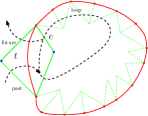
Figure 5: The envelope of an F symbol matched to a c. The green quadrangle corresponds to the F and its match. All the other blue edges on the boundary of the envelope correspond to the symbols H in the reduced word $\mathcal{R}$. Note that not all triangles on the boundary of the envelope are part of the loop itself. Right: the corresponding map if the F symbol is matched with an h.

We now describe an explicit exploration procedure of an envelope, starting from its F symbol, and exploring towards the past.

Exploration into the past for an envelope.

We start with a single edge $e$ and we explore the symbols strictly to the left of the F symbol. At every step we reveal a part of the map incident to an edge which we explore.

1. If the symbol is a $\textsf{C},\textsf{H}$ or a $\textsf{c},\textsf{h}$ which is not the match of the F, then we glue a single triangle to the edge we explore as in the right hand side of Figure 4.

2. If the symbol is an F, we explore its envelope and glue the corresponding map as explained above (see Figure 5). The refined edge corresponding to the “future” in Figure 5 is identified with the edge we are exploring and the edge corresponding to the “past” is the edge we explore next.

3. If the symbol is a c or h and is a match of the F symbol we started with, we finish the exploration as follows. Notice that in this situation, if the symbol is a c (or h) then the edge we explore is incident to $e$ via a dual (or primal) vertex. We now glue a primal (or dual) quadrangle with two of its adjacent refined edges identified with $e$ and the edge we explore. This step corresponds to adding the quadrangle with solid lines in Figure 5.

Remark 2.3.

We remark that it is possible to continue the exploration procedure above for the whole infinite word to the left of $X_{0}$. The only added subtlety is that some productions have a match to the right of $0$ and hence remain uneaten. The whole exploration thus produces a half planar map with boundary formed by these uneaten productions. However this information does not reveal all the decorations in the boundary since some of the boundary triangles might be matched by an F to the right of $X_{0}$.

We now explain how to extract information about the length and area of the loop given the symbols in an envelope. A preliminary observation is that the envelopes are nested. More precisely, if $X_{i}=\textsf{F}$ and $X_{j}=\textsf{F}$ for some $\varphi(i)<j<i$. Then $\mathsf{e}(X_{j})\subset\mathsf{e}(X_{i})$. To see this, observe that a positive number of burgers are produced between $X_{\varphi(i)}$ and $X_{i}$ and hence one of them must match $X_{j}$. Since it cannot be $X_{\varphi(i)}$ by definition, $\varphi(j)>\varphi(i)$.

If we define a partial order among the envelopes strictly contained in $\mathsf{e}(X_{i})$ then there exist maximal elements which we call maximal envelopes in $\mathsf{e}(X_{i})$.

Lemma 2.4.

Suppose $X_{i}=\textsf{F}$, and let $L$ be the corresponding loop. Then the following holds.

• The boundary of $\mathsf{e}(X_{i})$, that is the triangles in $\mathsf{e}(X_{i})$ which are adjacent to triangles in the complement of $\mathsf{e}(X_{i})$, consists of triangles in the reduced word $\overline{X_{\varphi(i)}\ldots X_{i}}$, plus one extra triangle (corresponding to $t$ in Figure 5). For an hF loop, the boundary consists of dual triangles corresponding to C symbols. An identical statement holds for an cF loop with dual replaced by primal.

• Let $\mathcal{M}$ denote the union of the maximal envelopes in $\mathsf{e}(X_{i})$ and let $m$ denote the number of maximal envelopes in $\mathsf{e}(X_{i})$. Then the length of $L$ is $m$ plus the number of triangles in $\mathsf{e}(X_{i})\setminus\mathcal{M}$ minus $1$.

• All the envelopes in $\mathcal{M}$ of type opposite (resp. same) to that of $L$ belong to the interior (resp. exterior) of $L$.

Proof.

The boundary of $\mathsf{e}(X_{i})$ is formed of symbols that are going to be matched by symbols outside $[\varphi(i),i]$. Thus by definition, the boundary consists of the triangles associated with the reduced word $\overline{X_{\varphi(i)}\ldots X_{i}}$. Also for an hF loop, the boundary consists of C symbols only since if there was an H symbol, it would have been a match of $\varphi(i)$. An identical argument holds for a cF loop.

For the second assertion, suppose we start the exploration procedure for a loop going into the past as described above. For steps as in item $1$, it is clear that we add a single triangle to the loop. For steps as in item $2$, i.e. when we reveal the map corresponding to a maximal envelope $E$, we also add a single triangle to the loop. Indeed an envelope consists of a single triangle $t$ glued to a map bounded by a cycle of either primal or dual edges (see Figure 5). If we iteratively explore $E$, $t$ is part of the quadrangle we add in step $3$ of the above exploration and it is the triangle $t$ which is added to the loop. For steps as in item $3$, we also add one triangle to the loop. This concludes the proof of the second assertion.

Clearly, the triangles corresponding to a loop has primal vertices on one side and dual vertices on the other side of the loop. Suppose $X_{i}$ is hF type. Then, as for any such loop, it has dual (or C) vertices adjacent to its exterior. For the same reason, every hF type maximal envelope in $\mathsf{e}(X_{i})$ must have dual (or C) vertices adjacent to its exterior. None of its triangles belong to the loop by the second assertion, and it is adjacent to $L$. So the only possibility is that it lies in its exterior. The other case is similar, so the last assertion is proved. ∎

3 Preliminary lemmas

3.1 Forward-backward equivalence

In this section, we reduce the question of computing critical exponents on the decorated map to a more tractable question on certain functionals of the Hamburger Cheeseburger sequence coming from Sheffield’s bijection. This reduction involves elementary but delicate identities and probabilistic estimates which need to be done carefully. By doing so we describe the length and area by quantities which have a more transparent random walk interpretation and that we will be able to estimate in Section 4.

Modulo these estimates, we complete the proof of Theorem 1.1 at the end of Section 3.1. From now on throughout the rest of the paper, we fix the following notations:

Definition 3.1.

Fix $p\in(0,1/2)$. Define

$$\theta_{0}=2\arctan\left(\frac{1}{\sqrt{1-2p}}\right);\quad p_{0}=\frac{\pi}{2\theta_{0}}=\frac{\kappa^{\prime}}{8}.$$

Note that the value of $p_{0}$ is identical to the one in (1.4) (after applying simple trigonometric formulae). Also assume throughout in what follows that $\{X_{k}\}_{k\in\mathbb{Z}}$ is an i.i.d. sequence given by (2.3).

For any $k\in\mathbb{Z}$, we define a burger stack at time $k$ to be $((X_{j})_{j\leq k}:\varphi(j)>k)$ endowed with the natural order it inherits from $\{X_{k}\}_{k\in\mathbb{Z}}$. The maximal element in a burger stack is called the burger or symbol at the top of the stack. It is possible to see that almost surely burger stack at time $k$ contains infinite elements almost surely for any $k\in\mathbb{Z}$ (see [36]).

Define $T=\varphi(0)$, and let $E=\{X_{\varphi(0)}=\textsf{F}\}$. Let $J_{T}=\overline{X_{0}\ldots X_{T}}$. Let $|J_{T}|$ denote the number of symbols in $\overline{X_{0}\ldots X_{T}}$. Let $\mathcal{S}_{k}$ denote the burger stack at time $k$. Let $\mathbb{P}^{s}$ denote the probability measure $\mathbb{P}$ conditioned on $\mathcal{S}_{0}=s$. Note that conditioning on the whole past $\{X_{j}\}_{j\leq k}$ at a given time $k$ is equivalent to conditioning just on the burger stack $s$ at that time.

Theorem 3.2.

Let $T,E,J_{T}$ be as above and $p_{0}=\kappa^{\prime}/8$ be as in Definition 3.1. Fix $\varepsilon>0$. There exist positive constants $c=c(\varepsilon),C=C(\varepsilon)$ such that for all $n\geq 1,m\geq n(\log n)^{3}$, for any burger stack $s$,

1. $\frac{cn^{2p_{0}}}{n^{1+\varepsilon}m^{4p_{0}+\varepsilon}}\leq\mathbb{P}^{s}(T>m^{2},|J_{T}|=n,E)\leq\frac{Cn^{2p_{0}}}{n^{1-\varepsilon}m^{4p_{0}-\varepsilon}}$,

2. $\frac{c}{n^{2p_{0}+1+\varepsilon}}\leq\mathbb{P}^{s}(|J_{T}|=n,E)\leq\frac{C}{n^{2p_{0}+1-\varepsilon}}$,

3. $\frac{c}{m^{2p_{0}+\varepsilon}}\leq\mathbb{P}^{s}(T>m^{2}\cap E)\leq\frac{C}{m^{2p_{0}-\varepsilon}}$,

4. $c\left(\frac{n^{4p_{0}-\varepsilon}}{m^{4p_{0}+\varepsilon}}\right)\leq\mathbb{P}^{s}(T>m^{2}\big{|}|J_{T}|=n\cap E)\leq C\left(\frac{n^{4p_{0}+\varepsilon}}{m^{4p_{0}-\varepsilon}}\right)$,

5. For any $p\in(0,2p_{0}-\varepsilon)$,

   $$cn^{2p-2\varepsilon}\leq\mathbb{E}^{s}(T^{p}\big{|}|J_{T}|=n\cap E)\leq Cn^{2p+2\varepsilon}.$$

In particular all these bounds are independent of the conditioning on $\mathcal{S}_{0}=s$.

Remark 3.3.

A finer asymptotics than (iii) above is obtained in [26, Proposition 5.1]. More precisely, it is proved that $\mathbb{P}(T>n\cap E)$ is regularly varying with index $p_{0}=\kappa^{\prime}/8$.

Let us admit Theorem 3.2 for now and let us check how this implies Theorem 1.1. To do this we need to relate $T,E$ and $J_{T}$ to observables on the map. We now check some useful invariance properties which use the fact that there are various equivalent ways of defining a typical loop.

Proposition 3.4.

The following random finite words have the same law.

1. The envelope of the first F to the left of $X_{0}$. That is $\mathsf{e}(X_{i})$ where $i=\max\{j\leq 0,X_{j}=\textsf{F}\}$.

2. The envelope of the first c or h to the right of $0$ matched with an F. That is $\mathsf{e}(\varphi(\Sigma))$ where $\Sigma=\min\{j\geq 0:X_{j}\in\{\textsf{c},\textsf{h}\},X_{\varphi(j)}=\textsf{F}\}$.

3. The envelope of $X_{0}$ conditioned on $X_{0}$ being an F.

4. The envelope of $X_{\varphi(0)}$, conditioned on $X_{\varphi(0)}=\textsf{F}$.

Furthermore this is the limit law as $n\to\infty$ for the envelope of a F taken uniformly at random from an i.i.d. sequence $X_{1},\ldots,X_{2n}$ distributed as in (2.3) and conditioned on $\overline{X_{1}\ldots X_{2n}}=\emptyset$.

Proof.

Let $\mathcal{W}$ be the set of finite words $\{w_{0},\ldots,w_{n},w_{n}=\textsf{F},n=\varphi(0)\}_{n\geq 0}$ of any length, that end with an F and start by its match. For $w=(w_{0},\ldots,w_{n})\in\mathcal{W}$, let $p(w)=\prod_{i=0}^{n}\mathbb{P}(X=w_{i})$. Let $p_{\mathcal{W}}(w)=p(w)/Z$ where $Z=\sum_{w\in\mathcal{W}}p(w)$. Clearly, $Z=\mathbb{P}(X=\textsf{F})=p/2$, since $\sqcup_{w\in\mathcal{W}}\{X_{-n}=w_{0},\ldots,X_{0}=w_{n}\}=\{X_{0}=\textsf{F}\}$ and these events are disjoint.

Note that the word in the item iii has a law given by $\mathbb{P}(e(X_{0})=w|X_{0}=\textsf{F})=(2/p)\prod_{i=0}^{n}\mathbb{P}(X=w_{i})=p_{\mathcal{W}}(w)$. This is also true of the word in the item i, since the law to the sequence to the left of the first F left of $0$ is still i.i.d.

Similarly, for the word in the item iv, conditioning on $X_{\varphi(0)}=\textsf{F}$ is the same thing as conditioning on $\mathsf{e}(X_{\varphi(0)})\in\mathcal{W}$ hence it follows that the random word has law $p_{\mathcal{W}}$ too. This then immediately implies the result in the item ii, since conditioned on the $k$th burger produced after time $0$ to be the first one eaten by an F, the envelope of the $k$th burger produced has law $p_{\mathcal{W}}$, independently of $k$.

The final assertion is a consequence of polynomial decay of empty reduced word as described in [36, 15] which we provide for completeness. For $w\in\mathcal{W}$ be a word with $k$ symbols. Let $N_{w}$ be the number of F symbols in $X_{1},\ldots,X_{n}$ such that its envelope is given by $w$. Let $N_{\textsf{F}}$ denote the number of F symbols in $X_{1},\ldots,X_{n}$. We can treat both $N_{\textsf{F}}$ and $N_{w}$ as empirical measure of states $w$ and F of certain Markov chains of length $n-k$ and $n$ respectively. By Sanov’s theorem,

$$\mathbb{P}(|\frac{N_{w}}{n}-p(w)|>\varepsilon)\leq ce^{-c^{\prime}n}\quad;\quad\mathbb{P}(|\frac{N_{\textsf{F}}}{n}-p/2|>\varepsilon)\leq ce^{-c^{\prime}n}$$

Since $\mathbb{P}(\overline{X_{1}\ldots X_{2n}})=\emptyset)=n^{-1-\kappa/4+o_{n}(1)}$ [27], our result follows. See for example [15] for more precise treatment of similar arguments. ∎

Let $(M_{n},T_{n})$ be as in eq. 2.1 and let $L_{n}$ be a uniformly picked loop from it. One can extend the definition of length, area, exterior and interior in Definition 2.2 to finite maps by adding the convention that the exterior of a loop is the component of the complement containing the root. (If the loop intersects the root edge, we define the interior to be empty.) Let $\mathcal{L}_{n}$ be the submap of $(\bar{M}_{n},\bar{T}_{n})$ formed by the triangles corresponding to the loop $L_{n}$ and the triangles in its interior. Recall that by definition, the length of the loop, denoted $\textsf{Len}(L_{n})$ is the number of triangles in $(\bar{M}_{n},\bar{T}_{n})$ present in the loop and the area $\textsf{Area}(L_{n})$ is the number of triangles in $\mathcal{L}_{n}$, that is, the number of triangles in the interior of the loop plus $\textsf{Len}(L_{n})$.

Proposition 3.5.

The number of triangles in $\mathcal{L}_{n}$ is tight and $\mathcal{L}_{n}$ converges to a finite map $\mathcal{L}$. The submap corresponding to triangles in $L_{n}$ converges to a map $L$. Also

• $\textsf{Len}(L_{n})\xrightarrow[]{n\to\infty}\textsf{Len}(L)$

• $\textsf{Area}(L_{n})\xrightarrow[]{n\to\infty}\textsf{Area}(L)$

where $\textsf{Len}(L)$ is the number of triangles in $L$ and $\textsf{Area}(L)$ is the number of triangles in $\mathcal{L}$. Further the law of $\textsf{Len}(L)$ and $\textsf{Area}(L)$ can be described as follows. Take an i.i.d. sequence $\{X_{i}\}_{i\in\mathbb{Z}}$ as in eq. 2.3 and condition on $X_{0}=\textsf{F}$. Then the map corresponding to $\mathsf{e}(X_{0})$ has the same law as $\mathcal{L}$. Thus the law of $\textsf{Len}(L)$ and $\textsf{Area}(L)$ can be described in the way prescribed by Lemma 2.4.

Proof.

Notice that there is a one to one correspondence between the number of F symbols in the finite word corresponding to $(M_{n},T_{n})$ except there is one extra loop. But since the number of F symbols in the finite word converges to infinity, the probability that we pick this extra loop converges to $0$. The rest follows from the last statement in Propositions 3.4 and 2.4. ∎

We now proceed to the proof of Theorem 1.1. We compute each exponent separately. In this proof we will make use of certain standard type exponent computations for i.i.d. heavy tailed random variables. For clarity, we have collected these lemmas in appendix A.

Proof of length exponent in Theorem 1.1.

We see from Proposition 3.5 that it is enough to condition on $X_{0}=\textsf{F}$ and look at the length of the loop and area of the envelope $\mathsf{e}(X_{0})$ as defined in Definition 2.2. We borrow the notations from Proposition 3.5. We see from the second item of Lemma 2.4, to get a handle on $\textsf{Len}(L)$, we need to control the number of maximal envelopes and the number of triangles not in maximal envelopes inside $\mathsf{e}(X_{0})$. To do this, we define a sequence $(c_{n},h_{n})_{n\geq 1}$ using the exploration into the past for an envelope as described in Section 2.4 and keeping track of the number of C and H in the reduced word. Let $(c_{0},h_{0})=(0,0)$. Suppose we have performed $n$ steps of the exploration and defined $c_{n},h_{n}$ and in this process, we have revealed triangles corresponding to symbols $(X_{-m},\ldots,X_{0})$. We inductively define the following.

• If $X_{-m-1}$ is a C (resp. H), define $(c_{n+1},h_{n+1})=(c_{n},h_{n})+(1,0)$ (resp. $(c_{n},h_{n})+(0,1)$).

• If $X_{-m-1}$ a c (resp. h), $(c_{n+1},h_{n+1})=(c_{n},h_{n})+(-1,0)$ (resp. $(c_{n},h_{n})+(0,-1)$).

• If $X_{-m-1}$ is F, then we explore $X_{-m-2},X_{-m-3}\ldots$ until we find the match of $X_{-m-1}$. Notice that the reduced word $\mathcal{R}_{n+1}=\overline{X_{\varphi(-m-1)}\ldots X_{-m-1}}$ is either of the form $\textsf{C}\textsf{C}\ldots\textsf{C}$ or $\textsf{H}\textsf{H}\ldots\textsf{H}$ depending on whether the match of the F is a h or c respectively. Either happens with equal probability by symmetry. Let $|\mathcal{R}_{n+1}|$ denote the number of symbols in the reduced word $\mathcal{R}_{n+1}$. If $\mathcal{R}_{n+1}$ consists of H symbols, define $(c_{n+1},h_{n+1})=(c_{n},h_{n})+(0,|\mathcal{R}_{n+1}|)$. Otherwise, if $\mathcal{R}_{n+1}$ consists of C symbols define $(c_{n+1},h_{n+1})=(c_{n},h_{n})+(|\mathcal{R}_{n+1}|,0)$.

For future reference, we call this exploration procedure the reduced walk.

Observe that the time $\varphi(0)$ where we find the match of 0 in the reduced walk is precisely the time $n$ when the process $(c_{n},h_{n})$ leaves the first quadrant, i.e., $\tau:=\inf\{k:c_{k}\wedge h_{k}<0\}$. This is because $\tau$ is the first step when $\overline{X_{-\tau}\ldots X_{-1}}$ consists of a c or h symbol followed by a (possibly empty) sequence of burger orders of the opposite type and hence the c or h produced is the match of F at $X_{0}$. Also from second item of Lemma 2.4, $\tau$ is exactly the number of triangles in the loop (as exploring the envelope of each F corresponds to removing the maximal envelopes in the loop of $X_{0}$).

We observe that the walk $(c_{n},h_{n})$ is just a sum of i.i.d. random variables which are furthermore centered. Indeed, conditioned on the first coordinate being changed, the expected change is $0$ via (2.3) and the computation by Sheffield [36] which boils down to the fact that $\mathbb{E}(|\mathcal{R}|)=1$ (this is the quantity $\chi-1$ in [36], which is 1 when $q\leq 4$)

Although the change in one coordinate means the other coordinate stays put, estimating the tail of $\tau$ is actually a one-dimensional problem since the coordinates are essentially independent. Indeed if instead of changing at discrete times, each coordinate jumps in continuous time with a Poisson clock of jump rate $1$, the two coordinates becomes independent (note that this will not affect the tail exponent by standard concentration arguments). Let $\tau^{c}$ be the return time to $0$ of the first coordinate. By this argument, $\mathbb{P}(\tau>k)=\mathbb{P}(\tau^{c}>k)^{2}$. Now, $|\mathcal{R}|$ has the same distribution as $J_{T}$ conditionally given $X_{\varphi(0)}=\textsf{F}$, by Proposition 3.4 equivalence of items iii and iv. It is a standard fact that the return time of a heavy tailed walk with exponent $\alpha$ has exponent $1/\alpha$. In our slightly weaker context, we prove this fact in Lemma A.2. It follows that $\mathbb{P}(\tau^{c}>k)=k^{-1/(2p_{0})+o(1)}$ and hence $\mathbb{P}(\tau>k)=k^{-1/p_{0}+o(1)}$. This completes the proof of the tail asymptotics for the length of the loop. ∎

Proof of area exponent in Theorem 1.1.

For the lower bound, let us condition on $X_{0}=\textsf{F}$ and set $T^{\prime}=-\varphi(0)$. Then we break up $T^{\prime}$ as $T^{\prime}=\sum_{n=1}^{\tau}(T^{c}_{n}+T^{h}_{n})$ defined as follows. In every reduced walk exploration step, if the walk moves in the first coordinate, then $T^{c}_{n}$ denotes the number of triangles explored in this step otherwise $T^{c}_{n}=0$. Also $T^{h}_{n}$ is defined in a similar way. Hence $T_{n}^{c}+T_{n}^{h}$ counts the number of symbols explored in step $n$ of the reduced walk. Observe further that translating Lemma 2.4 (third item) to this context and these notations, we have that $\textsf{Area}(L)=\sum_{n=1}^{\tau}T_{n}^{c}$ or $\textsf{Area}(L)=\sum_{n=1}^{\tau}T_{n}^{h}$ depending on which coordinate hits zero first (if $\tau=\tau^{c}$ then $\textsf{Area}(L)=\sum_{n=1}^{\tau}T_{n}^{c}$ and vice-versa).

Now notice that $T_{n}^{c/h}$ has a probability bounded away from zero to make a jump of size at least $k$ in every $k^{p_{0}+\varepsilon}$ steps, by Theorem 3.2. Hence using the Markov property and a union bound over cheese and hamburgers,

$$\mathbb{P}(\sum_{i=1}^{k^{p_{0}+2\varepsilon}}T^{c}_{i}\leq k\text{ or }\sum_{i=1}^{k^{p_{0}+2\varepsilon}}T^{h}_{i}\leq k)\leq e^{-ck^{\varepsilon}}.$$ (3.1)

Hence

$$\mathbb{P}(\textsf{Area}(L)>k)\geq\mathbb{P}(\textsf{Area}(L)>k,\tau>k^{p_{0}+2\varepsilon})\geq\mathbb{P}(\tau>k^{p_{0}+2\varepsilon})-e^{-ck^{\varepsilon}}\geq k^{-1-2\varepsilon+o(1)}$$ (3.2)

Now we focus on the upper bound. Since the coordinates are symmetric, it is enough to prove

$$\mathbb{P}(\sum_{n=1}^{\tau^{c}}T_{n}^{c}>k,\,\tau=\tau^{c})\leq k^{-1+\varepsilon+o(1)}.$$ (3.3)

Since $\mathbb{P}(\tau>k^{p_{0}})=k^{-1+o(1)}$, we can further restrict ourselves to the case $\tau\leq k^{p_{0}}$. Now roughly the idea is as follows. When we condition on the event $\{\tau=\tau^{c}=j\}$ with $j\leq k^{p_{0}}$, there are several ways in which the area can be larger than $k$.

One way is if the the maximal jump size of $(|\mathcal{R}_{i}|)_{1\leq i\leq j}$ is itself large, in which case there is a maximal envelope with a large boundary (and therefore a large area).

The second way is if the maximal jump size is small and the area manages to be large because of many medium size envelopes, but we are able to discard it by comparing a sum of heavy-tailed random variables to its maximum.

Therefore, the following third way will be the more common. We will see that the maximal jump size in $|\mathcal{R}_{i}|$ is at most $j^{\frac{1}{2p_{0}}}$ with exponentially high probability, even though the $\mathcal{R}_{i}$ are heavy-tailed. Now, if the area is to be large (greater than $k$) and one maximal envelope contains essentially all of the area, then the area of that envelope will have to be big compared to its boundary. We handle this deviation by using a Markov inequality with a nearly optimal power and item v in Theorem 3.2.

We first convert the problem to a one-dimensional problem. To this end let $\xi_{n}=c_{n}-c_{n-1}$, i.e., we look at the jumps only restricted to the cheeseburger coordinate. We now observe that on the event $\tau^{c}=k$, we have $\xi^{*}:=\sup_{n\leq\tau^{c}}\xi_{n}\leq k^{\frac{1}{2p_{0}}+\delta}$ with probability at least $1-ke^{-ck^{\delta}}$. To see this we use the following exponential left tail of sums of $\xi_{n}$ (see Lemma A.1 for a proof; in words, a big jump is exponentially unlikely on the event $\tau^{c}=j$ because if there is one, the walk has to come down to $0$ very fast)

$$\mathbb{P}(\sum_{n=1}^{k}\xi_{n}<-\lambda k^{\frac{1}{2p_{0}}+\delta})\leq 2e^{-c(\delta)\lambda}.$$ (3.4)

Using all this, it is enough to show, with $\delta=\varepsilon/4$ say,

$$\mathbb{P}(\sum_{n=1}^{\tau^{c}}T_{n}^{c}>k,\xi^{*}\leq(\tau^{c})^{\frac{1}{2p_{0}}+\delta},\,\tau=\tau^{c}\leq k^{p_{0}})\leq k^{-1+\varepsilon+o(1)}.$$ (3.5)

Let $T_{j}^{*}=\max_{1\leq n\leq j}T_{n}^{c}$. Using Markov’s inequality, for all $\varepsilon>0,\delta=\varepsilon/4$,

$$\mathbb{P}(\sum_{n=1}^{\tau^{c}}T_{n}^{c}>k, \,\xi^{*}\leq(\tau^{c})^{\frac{1}{2p_{0}}+\delta},\,\tau=\tau^{c}\leq k^{p_{0}})$$

$$\leq\frac{C(\varepsilon)}{k^{2p_{0}-\varepsilon}}\sum_{j=1}^{k^{p_{0}}}\mathbb{E}\left((\sum_{n=1}^{j}T_{n}^{c})^{2p_{0}-\varepsilon}\mathbbm{1}_{\xi^{*}\leq j^{\frac{1}{2p_{0}}+\delta}},\mathbbm{1}_{\tau=\tau^{c}=j}\right)$$

$$\leq\frac{1}{k^{2p_{0}-\varepsilon}}\sum_{j=1}^{k^{p_{0}}}\mathbb{E}\left(\left(\frac{\sum_{n=1}^{j}T_{n}^{c}}{(T_{j}^{*})^{1+\delta}}\right)^{2p_{0}-\varepsilon}\left((T_{j}^{*})^{1+\delta}\right)^{2p_{0}-\varepsilon}\mathbbm{1}_{\xi^{*}\leq j^{\frac{1}{2p_{0}}+\delta}},\mathbbm{1}_{\tau=\tau^{c}=j}\right)$$ (3.6)

It is a standard fact that for heavy tailed variables with infinite expectation, the sum is of the order of its maximum with exponentially high probability. This is stated and proved formally in Lemma A.3. Using this fact, Holder’s inequality and the fact that $(1+\delta)(2p_{0}-\varepsilon)<2p_{0}-\varepsilon/2$ we conclude that

$$\mathbb{P}(\sum_{n=1}^{\tau^{c}}T_{n}^{c}>k,\,\xi^{*}\leq(\tau^{c})^{\frac{1}{2p_{0}}+\delta},\,\tau=\tau^{c}\leq k^{p_{0}}) \leq\frac{C(\varepsilon)}{k^{2p_{0}-\varepsilon}}\sum_{j=1}^{k^{p_{0}}}\mathbb{E}\left((T_{j}^{*})^{2p_{0}-\varepsilon/4}\mathbbm{1}_{\xi^{*}\leq j^{\frac{1}{2p_{0}}+\delta}},\mathbbm{1}_{\tau=\tau^{c}=j}\right)$$

$$\leq\frac{C(\varepsilon)}{k^{2p_{0}-\varepsilon}}\sum_{j=1}^{k^{p_{0}}}\mathbb{E}\left(\sum_{1\leq n\leq j}(T_{n}^{c})^{2p_{0}-\varepsilon/4}\mathbbm{1}_{\xi^{*}\leq j^{\frac{1}{2p_{0}}+\delta}},\mathbbm{1}_{\tau=\tau^{c}=j}\right)$$

Now let $\mathcal{G}$ be the $\sigma$-algebra generated by $(\mathcal{R}_{n})_{n\geq 0}$. Notice that $\tau^{c},\tau^{h}$, $\xi^{*}$ are $\mathcal{G}$-measurable and that $T_{n}^{c}$ is independent of $(\mathcal{R}_{i})_{i\neq n}$. Also notice from item v of Theorem 3.2 that $\mathbb{E}((T_{n}^{c})^{2p_{0}-\varepsilon/4}|\mathcal{G})\leq C(\varepsilon)|\mathcal{R}_{n}|^{4p_{0}-\varepsilon/4}\mathbbm{1}_{\xi_{n}>0}$. Thus we conclude

$$\mathbb{P}(\sum_{n=1}^{\tau^{c}}T_{n}^{c}>k,\,\xi^{*}\leq(\tau^{c})^{\frac{1}{2p_{0}}+\delta},\,\tau=\tau^{c}\leq k^{p_{0}}) \leq\frac{C(\varepsilon)}{k^{2p_{0}-\varepsilon}}\sum_{j=1}^{k^{p_{0}}}\mathbb{E}\left(\sum_{1\leq n\leq j}|\mathcal{R}_{n}|^{4p_{0}-\varepsilon/4}\mathbbm{1}_{\xi_{n}>0},\mathbbm{1}_{\xi^{*}\leq j^{\frac{1}{2p_{0}}+\delta}},\mathbbm{1}_{\tau=\tau^{c}=j}\right)$$

Again using Holder and Lemma A.3 similar to (3.6), we can replace $\sum_{1\leq n\leq j}|\mathcal{R}_{n}|^{4p_{0}-\varepsilon/4}\mathbbm{1}_{\xi_{n}>0}$ by $(\xi^{*})^{4p_{0}-\varepsilon/8}$ in the above expression and obtain that the right hand side above is at most (moving to continuous time to get independence of $\tau^{c}$ and $\tau^{h}$ as in the earlier proof of the length exponent),

$$\frac{C(\varepsilon)}{k^{2p_{0}-\varepsilon}}\sum_{j=1}^{k^{p_{0}}}\mathbb{E}\left((\xi^{*})^{4p_{0}-\varepsilon/8}\mathbbm{1}_{\xi^{*}\leq j^{\frac{1}{2p_{0}}+\delta}},\mathbbm{1}_{\tau=\tau^{c}=j}\right) \leq\frac{C(\varepsilon)}{k^{2p_{0}-\varepsilon}}\sum_{j=1}^{k^{p_{0}}}j^{2+\varepsilon}\mathbb{P}(\tau^{c}=j)\mathbb{P}(\tau^{h}>j)$$

$$\leq\frac{C(\varepsilon)}{k^{2p_{0}-\varepsilon}}\sum_{j=1}^{k^{p_{0}}}j^{1+2\varepsilon-\frac{1}{p_{0}}}$$

$$\leq\frac{C(\varepsilon)}{k^{2p_{0}-\varepsilon}}(k^{p_{0}})^{2-\frac{1}{p_{0}}+2\varepsilon}=k^{-1+3\varepsilon+o(1)}$$

as desired. ∎

3.2 Connection with random walk in cone

Given the sequence $\{X_{i}\}_{i\in\mathbb{Z}}$ and $\mathcal{S}_{0}$, the burger stack at time $0$, we can construct the sequence $\{\hat{X}_{i}\}_{i\in\mathbb{Z}}$ where we convert every F symbol in $\{X_{i}\}_{i\in\mathbb{Z}}$ into the corresponding C symbol or H symbol.

Define $(U^{x}_{n})_{n\geq 1}$ to be the algebraic cheeseburger count as follows:

$$U^{x}_{i}-U^{x}_{i-1}=\begin{cases}+1&\text{ if }\hat{X}_{i}=\textsf{c},\\ -1&\text{ if }\hat{X}_{i}=\textsf{C},\\ 0&\text{ otherwise.}\end{cases}$$ (3.7)

Similarly define the hamburger count $U^{y}_{i}$ by letting its increment $U^{y}_{i}-U^{y}_{i-1}$ be $\pm 1$ depending whether $\hat{X}_{i}=\textsf{h},\textsf{H}$ or 0 otherwise.

Recall our notation $p$ defined in eq. 2.3 so that $p/2=\mathbb{P}(\textsf{F})$. The main result of Sheffield [36], which we rephrase for ease of reference later on, is as follows.

Theorem 3.6 (Sheffield [36]).

Conditioned on any realisation of $\mathcal{S}_{0}$, we have the following convergence uniformly in every compact interval

$$\left(\frac{U^{x}_{\lfloor nt\rfloor}}{\sqrt{n}},\frac{U^{y}_{\lfloor nt\rfloor}}{\sqrt{n}}\right)_{t\geq 0}\xrightarrow[]{n\to\infty}(L_{t},R_{t})_{t\geq 0}$$

where $(L_{t},R_{t})_{t\geq 0}$ evolves as a two-dimensional correlated Brownian motion with $\operatorname{Var}(L_{1})=\operatorname{Var}(R_{1})=(1-p)/2=\sigma^{2}$ and $\operatorname{Cov}(L_{1},R_{1})=p/2$.

Remark 3.7.

Up to a scaling, this Brownian motion $(L_{t},R_{t})_{t\geq 0}$ is exactly the same which arises in the main result of [20] (Theorem 9.1). This is not surprising: indeed, the hamburger and cheeseburger count give precisely the relative length of the boundary on the left and right of the space-filling exploration of the map.

In order to work with uncorrelated Brownian motions, we introduce the following linear transformation $\Lambda$:

$$\Lambda=(1/\sigma)\left(\begin{array}[]{cc}1&\cos(\theta_{0})\\ 0&\sin(\theta_{0})\end{array}\right)$$

where $\theta_{0}=\pi/(2p_{0})=4\pi/\kappa^{\prime}=2\arctan(\sqrt{1/(1-2p)}$ and $\sigma^{2}=(1-p)/2$ as in the above theorem. A direct but tedious computation shows that $\Lambda(L_{t},R_{t})$ is indeed a standard planar Brownian motion. (The computation is easier to do by reverting to the original formulation of Theorem 3.6 in [36], where it is shown that $U^{x}+U^{y}$ and $(U^{x}-U^{y})/\sqrt{1-2p}$ form a standard Brownian motion; however this presentation is easier to understand for what follows).

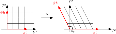
Figure 6: The coordinate transformation. Note that in the new coordinates, leaving the cone $\mathcal{C}(\theta_{0})$ (in red in the picture) at some time $n$ corresponds to having eaten all burgers of a given type between times 0 and $n$.

We now perform the change of coordinates in the discrete, and thus define for $n\geq 0$, $\boldsymbol{V}_{n}=(V^{x}_{n},V^{y}_{n})=\Lambda(U^{x}_{n},U^{y}_{n})$ (see Figure 6). We define $\boldsymbol{v}_{0}=\Lambda(0,1)$ (note that argument of $\boldsymbol{v}_{0}$ is the same as that of the cone). Let $\mathcal{C}(\theta):=\{(r,\eta):r\geq 0,\eta\in[0,\theta]\}$ denote the $2$-dimensional closed cone of angle $\theta$ and let $\mathcal{C}_{n}(\theta)$ be the translate of the cone $\mathcal{C}(\theta)$ by the vector $-n\boldsymbol{v}_{0}$. Now define $T^{*}_{\theta_{0},n}(\boldsymbol{V}):=\min\{k\geq 1,\boldsymbol{V}_{k}\notin\mathcal{C}_{n}(\theta_{0})\}$. Let $E^{*}_{n}$ denote the event that

$$E^{*}_{n}=(X_{0}=\textsf{c})\cap(\boldsymbol{V}_{T^{*}_{\theta_{0},n}-1}=-n\boldsymbol{v}_{0})\cap(X_{T^{*}_{\theta_{0},n}}=\textsf{F})$$

In words, the walk leaves the cone $\mathcal{C}_{n}(\theta_{0})$ through its tip, and the symbol at this time is an F. Recall the event $E=\{X_{\varphi(0)}=\textsf{F}\}$.

Lemma 3.8.

The events $\{X_{0}=\textsf{c}\}\cap\{T>m^{2},|J_{T}|=n\}\cap E$ and $E^{*}_{n}\cap\{T_{\theta_{0},n}^{*}>m^{2}\}$ are identical.

Proof.

Consider $(U^{x},U^{y})$ for a moment and suppose $X_{0}=\textsf{c}$. Observe that $\varphi(0)$ corresponds to the first time that $U^{x}=-1$. Moreover, the set of times $t\leq\varphi(0)$ such that $U_{t}^{x}=0$ corresponds to the times at which that initial cheeseburger is the top cheeseburger on the stack; and the size of the infimum, $|\inf_{s\leq t}U^{y}_{s}|$ gives us the number of hamburger orders which have its match at a negative time; or in other words, the number of hamburger orders H in the reduced word at time $t$.

Now the event $E$ occurs if and only if the burger at $X_{0}$ gets to the top of the stack and this is immediately followed by an F. Hence the event $E\cap(|J_{T}|=n)$ will occur if and only if $U_{t}^{y}=\inf_{s\leq t}U^{y}_{s}=-n$ and $U^{x}_{t}=\inf_{s\leq t}U^{x}_{s}=0$ for some $t$, and we have an F immediately after. In other words, the walk $(U^{x},U^{y})$ leaves the quadrant $\{x\geq 0,y\geq-n\}$ for the first time at time $t$, and does so through the tip. Equivalently, applying the linear map $\Lambda$, $\boldsymbol{V}$ leaves the cone $\mathcal{C}_{n,\theta_{0}}$ for the first time at time $t$, and does so through the tip. ∎

4 Random walk estimates

We call $\Lambda(\mathbb{Z}^{2})$ the lattice points, which are the points that $\boldsymbol{V}$ can visit. Let $s$ be an infinite burger stack and let $x$ be a lattice point. From now on we denote by $\mathbb{P}^{x,s}$ the law of the walk $\boldsymbol{V}$ started from $x$ conditioned on $\mathcal{S}_{0}=s$. In this section, we prove the following lemma. Recall $p_{0}=\pi/2\theta_{0}$ from Definition 3.1.

Proposition 4.1.

For all $\varepsilon>0$ there exist positive constants $c=c(\varepsilon),C=C(\varepsilon)$ such that for all $n\geq 1$, all $m\geq n(\log n)^{3}$, and any infinite burger stack $s$,

$$\frac{cn^{2p_{0}}}{n^{1+\varepsilon}m^{4p_{0}+\varepsilon}}\leq\mathbb{P}^{0,s}(E^{*}_{n};T^{*}_{\theta_{0},n}>m^{2})\leq\frac{Cn^{2p_{0}}}{n^{1-\varepsilon}m^{4p_{0}-\varepsilon}}$$ (4.1)

Furthermore,

$$\frac{c}{n^{2p_{0}+1+\varepsilon}}\leq\mathbb{P}^{0,s}(E^{*}_{n})\leq\frac{C}{n^{2p_{0}+1-\varepsilon}}.$$ (4.2)

Using Lemma 3.8 and the symmetry betweeen cheese and hamburgers, the above lemma completes the proof of the first item of Theorem 3.2.

4.1 Sketch of argument in Brownian case.

To ease the explanations we will first explain heuristically how the exponent can be computed, discussing only the analogous question for a Brownian motion. To start with, consider the following simpler question. Let $B$ be a standard two-dimensional Brownian motion started at a point with polar coordinate $(1,\theta_{0}/2)$ and let $S$ be the first time that $B$ leaves $\mathcal{C}(\theta_{0})$. For this we have:

$$\mathbb{P}(S>t)=t^{-p_{0}+o(1)}$$ (4.3)

as $t\to\infty$. To see why this is the case, consider the conformal map $z\mapsto z^{\pi/\theta_{0}}.$ This sends the cone $\mathcal{C}(\theta_{0})$ to the upper-half plane. In the upper-half plane, the function $z\mapsto\Im(z)$ is harmonic with zero boundary condition. We deduce that, in the cone,

$$z\mapsto g(z):=r^{\pi/\theta_{0}}\sin\left(\frac{\pi\theta}{\theta_{0}}\right);\quad z\in\mathcal{C}(\theta_{0}),$$

is harmonic.

Now in the cone $\mathcal{C}_{n}(\theta_{0})$, if Brownian motion survives for a time $m^{2}\gg n^{2}$, then it is plausible that it reaches distance at least $m$ from the tip of $\mathcal{C}_{n}(\theta_{0})$. We are interested in the event that the Brownian motion reaches distance $m$ from the tip of $\mathcal{C}_{n}(\theta_{0})$ before reaching near the tip of $\mathcal{C}_{n}(\theta_{0})$ while staying inside the cone.

We now decompose this event into three steps. In the first step, the Brownian motion must first reach a distance $n/2$ from the origin. This is like surviving in the upper half plane which by the heuristics above has probability roughly $n^{-1}$. In the second step, the walk reaches distance $m$ with probability roughly $(n/m)^{2p_{0}}$. This can be deduced by using the harmonic function above which grows like $r^{2p_{0}}$.

Finally for the third step, the Brownian motion must go back to the tip. Suppose now, that we are interested in the event $\mathcal{E}$ that the Brownian motion leaves the cone $\mathcal{C}(\theta_{0})$ through the ball of radius 1, that is, $\mathcal{E}=\{|B_{S}|\leq 1\}$. To compute the tail of $S$ on this event, we can use the function

$$z\mapsto g(z):=r^{-\pi/\theta_{0}}\sin\left(\frac{\pi\theta}{\theta_{0}}\right);z\in\mathcal{C}(\theta_{0}),$$

which is harmonic for the same reason as above (note that the sign of the exponent in the power of $r$ is now opposite of what it was before (we flipped the images of $0$ and $\infty$ in the choice of the conformal map). Using this we can conclude that coming back to the ball of radius $1$ from distance $m$ costs $m^{-2p_{0}}$.

Thus combining all the three steps, we obtain $n^{-1}\cdot(n/m)^{2p_{0}}\cdot m^{-2p_{0}}$ which is roughly what is claimed in Proposition 4.1.

4.2 Cone estimates for random walk

We want to replace the Brownian motion in the above sketch by a random walk. The difficulty here is that the functions $r^{\pm\pi/\theta_{0}}\sin(\frac{\pi\theta}{\theta_{0}})$ are not exactly harmonic for the random walk. The main idea to overcome this is to approximate the Brownian motion by large blocks of the walk $\boldsymbol{V}$, of an appropriate macroscopic length (see Definition 4.2) for which the central limit theorem will apply. To deal with the small error in this approximation, we have to give ourself some room by perturbing the above functions so that they become strictly sub-harmonic or super-harmonic and this explains why we lose an $\varepsilon$ in the exponent (see Proposition 4.3). Once we know how to get sub-martingale and super-martingale for the walk, the rest follows quite easily. This is similar to a strategy originally devised by McConnell [30], with some small but crucial differences.

Now we begin the proof of Proposition 4.1. Recall that $\Lambda(\mathbb{Z}^{2})$ is the set of lattice points where $\boldsymbol{V}$ can visit. For $x>0$ and a process $(Z_{k})_{k\geq 0}$ define

$$T_{\theta_{1},\theta_{2}}^{*}=T_{\theta_{1},\theta_{2}}^{*}(Z):=\min\{k\geq 1,Z_{k}\notin\mathcal{C}(\theta_{1},\theta_{2})\}.$$

We sometimes denote $T^{*}_{\theta}$ for $T^{*}_{0,\theta}$ when there is no source of confusion. Also recall the notation $T^{*}_{\theta_{0},n}$ from Lemma 3.8.

Definition 4.2.

For $\varepsilon>0$ we will define the following time-changed walk $\{Y_{i}(\varepsilon)\}_{i\geq 0}$ and stopping times $\{\tau_{i}(\varepsilon)\}_{i\geq 0}$ as follows. Start with $Y_{0}(\varepsilon)=\boldsymbol{V}_{0}$ and $\tau_{0}(\varepsilon)=0$. Given $\boldsymbol{V}_{\tau_{k}(\varepsilon)}=Y_{k}(\varepsilon)$, we inductively define $\tau_{k+1}(\varepsilon)=\min\{t>\tau_{k}(\varepsilon):|{\boldsymbol{V}}_{t}-{\boldsymbol{V}}_{\tau_{k}(\varepsilon)}|>\varepsilon|Y_{k}|\}$ and $Y_{k+1}(\varepsilon)=\boldsymbol{V}_{\tau_{k+1}}$.

The next proposition shows that the Brownian motion estimates in Section 4.1 pass through to the discrete walk estimates with $\varepsilon$ error using little more than the invariance principle. This proposition is the key step for transferring results from Brownian motion to the discrete walk. To help alleviate notations, and since $\varepsilon$ is fixed throughout this proposition we will simply write $\tau_{k}$, and $Y_{k}$ for $\tau_{k}(\varepsilon)$ and $Y_{k}(\varepsilon)$. Let $\mathcal{C}(\theta_{1},\theta_{2})=\{z:\theta_{1}<\arg(z)<\theta_{2}\}$.

Proposition 4.3.

Fix $\pi/2\leq\theta<\pi$ and an infinite burger stack $s$. Let $f:\mathbb{R}^{2}{\setminus\{0\}}\to\mathbb{R}$ be a continuous function such that

1. $\Delta f(x)>0$ (resp. $\Delta f(x)<0$) for all $x\in\mathcal{C}(\theta)$.

2. $f$ is homogeneous in the sense that $f(\lambda x)=\lambda^{d}x$ for some $d\in\mathbb{R}$ and all $\lambda>0$.

There exists $\varepsilon_{0}$ such that if $\varepsilon\in(0,\varepsilon_{0})$, the following holds. There exists a constant $r_{0}(\varepsilon)>0$ such that for all lattice points $v$ in $\mathcal{C}(\varepsilon,\theta-\varepsilon)$ with $|v|>r_{0}$, $f(Y_{k})$ is a $\mathbb{P}^{v,s}$ submartingale (resp. supermartingale) with respect to the filtration $\mathcal{F}_{k}=\sigma(X_{i}:1\leq i\leq\tau_{k})$ until the walk $Y$ exits $\mathcal{C}(\varepsilon,\theta-\varepsilon)\cap\{z:|z|>r_{0}\}$.

Proof.

First observe that it is enough to show that there exists an $r_{0}$ such that for any lattice point $v$ in $\mathcal{C}(2\varepsilon,\theta-2\varepsilon)$ with $|v|>r_{0}$ and any infinite burger stack $s$,

$$\mathbb{E}^{v,s}\big{(}f(Y_{1})\big{)}-f(v)>0$$ (4.4)

where $\mathbb{E}^{v,s}$ is the expectation with respect to the measure $\mathbb{P}^{v,s}$. This is because conditioned on $\mathcal{F}_{k}$, the sequence $\{\boldsymbol{V}_{\tau_{k}+i}\}_{i\geq 1}$ has the law $\mathbb{P}^{\boldsymbol{V}_{\tau_{k}},\mathcal{S}_{\tau_{k}}}$. Also notice that we stop when the walk $\boldsymbol{V}$ reaches a distance less than $r_{0}$ or leaves the cone $\mathcal{C}(2\varepsilon,\theta-2\varepsilon)$ and hence we only need to prove (4.4) when $v$ is in the claimed range.

The claim (4.4) is a consequence of the invariance principle and a result of Sheffield (Lemma 4.4 stated below). The important issue is to verify that we can pick an $r_{0}$ uniformly over the burger stack $s$ and the initial position of the walk $Y_{0}=v$. To establish this, we set up a few notations. For any continuous curve $\gamma$ let $\tau(\gamma,\varepsilon)$ denote the exit time of $\gamma$ from the ball $\{z:|z-x|<\varepsilon|x|\}$ where $x=\gamma(0)$. Let

$$Z(\gamma)=Z(\gamma,\varepsilon)=\gamma(\tau)\text{ where }\tau=\tau(\gamma,\varepsilon)$$ (4.5)

denote the position of the curve at time $\tau(\gamma,\varepsilon)$. Let $D=\overline{\mathcal{C}(2\varepsilon,\theta-2\varepsilon)}\cap\{|x|=1\}$ where $\overline{\mathcal{C}(2\varepsilon,\theta-2\varepsilon)}$ is the closure of $\mathcal{C}(2\varepsilon,\theta-2\varepsilon)$ (in particular, note that $D$ is compact). With these notations, observe that $\mathbb{E}^{v,s}[f(Y_{1})]=\mathbb{E}^{v,s}[f(Z(\boldsymbol{V}))]$, so our goal (4.4) becomes

$$\mathbb{E}^{v,s}\big{[}f(Z(\boldsymbol{V}))\big{]}>f(v).$$ (4.6)

Let $B$ denote a standard Brownian motion. A preliminary observation is that by our assumptions on $f$, $\mathbb{E}^{x}(f(Z(B)))-f(x)>0$ for all $x\in D$. Moreover, since the left hand side is obviously continuous in $x$, we deduce that there is a constant $\delta>0$ such that

$$\mathbb{E}^{x}\big{[}f(Z(B))\big{]}-f(x)>\delta,\quad\quad\forall x\in D.$$ (4.7)

Now we approximate $B$ by the discrete walk. Let $A(\varepsilon):=\{x:1-\varepsilon\leq|x|\leq 1+\varepsilon,0\leq\arg(x)\leq\theta\}$ and let $M=\max\{|f(x)|:x\in A(\varepsilon)\}$. First choose $K>0$ such that

$$\mathbb{P}^{x}(\tau(B,2\varepsilon)>K)<\frac{\delta}{16M}\quad\quad\forall x\in D.$$ (4.8)

Fix some arbitrary infinite burger stack $s$ for now. Choose $r_{0}(s)>0$ such that for all $v\in\mathcal{C}(\varepsilon,\theta-\varepsilon)\cap\Lambda(\mathbb{Z}^{2})$ with $|v|>r_{0}$, the following holds.

From the invariance principle (Theorem 3.6), we know that as $v\to\infty$, the distribution of $\boldsymbol{V}(\cdot|v|^{2})/|v|$ under $\mathbb{P}^{v,s}$ is close that of Brownian motion $B$ started from $v/|v|$, uniformly over $v$ by translation invariance. Hence for $v$ sufficiently large (i.e., there is $r_{0}=r_{0}(s)$ such that if $|v|>r_{0}(s)$), by uniform continuity of $f$ in the annulus $A(1/2)$,

$$\big{|}\mathbb{E}^{v,s}\big{[}f(Z(\tfrac{\boldsymbol{V}}{|v|}))\big{]}-\mathbb{E}^{v/|v|}\big{[}f(Z(B))\big{]}\big{|}<\delta/8.$$ (4.9)

For the same reason, if $|v|>r_{0}(s)$ then for $K$ as in (4.8),

$$\mathbb{P}^{v,s}\big{[}\tau(\boldsymbol{V},2\varepsilon)>K|v|^{2}\big{]})<\frac{\delta}{12M}.$$ (4.10)

Now we will show that the conclusion eq. 4.9 holds for $|v|>r_{0}(s)$ even if $s$ is changed into another infinite burger stack $s^{\prime}$. For this the main tool is the following estimate due to Sheffield (which was already at the heart of [36]).

Lemma 4.4 (Lemma 3.7 in [36]).

Let $F_{n}$ denote the number of F symbols in $\overline{X_{0}X_{1}\ldots X_{n}}$. Then for all $\varepsilon>0$,

$$\mathbb{P}\left(\frac{F_{n}}{\sqrt{n}}>\varepsilon\right)\to 0.$$

as $n\to\infty$.

Fix $\eta\in(0,\varepsilon/2)$ be such that for $x,y$ in the annulus $A(1/2)$ such that $|x-y|<2\eta$ we have $|f(x)-f(y)|<\delta/4$. Let $h<\eta$ be such that $\mathbb{P}^{x}[\sup_{\tau(B,\epsilon-h)\leq t_{1},t_{2}\leq\tau(B,\epsilon+h)}|B_{t_{1}}-B_{t_{2}}|>\eta/2]<\delta/(20M)$ for any $x\in\mathbb{R}^{2}$. Reasoning as in eq. 4.9 and eq. 4.10, we also have that

$$\mathbb{P}^{v,s}\left[\mathcal{H}\right]\leq\frac{\delta}{12M},\text{ where }\mathcal{H}=\left\{\sup_{t_{1},t_{2}\in[\tau(\boldsymbol{V},\varepsilon-h),\tau(\boldsymbol{V},\varepsilon+h)]}|\boldsymbol{V}_{t_{1}}-\boldsymbol{V}_{t_{2}}|>\eta|\boldsymbol{V}_{0}|\right\}$$ (4.11)

(Note for later use that since $\eta$ depends only on $\delta$, $h$ depends only on $\delta$ which depends only on $f$).

Using Lemma 4.4, we can assume that the choice of $r_{0}$ (depending only on $\delta,M$) is such that for all $r>r_{0}$, the number $F_{r}$ of F symbols in $\overline{X_{1}\ldots X_{r}}$ satisfies

$$\mathbb{P}(F_{r}>h\sqrt{r/K})\leq\frac{\delta}{12M}.$$ (4.12)

Let $v$ be a fixed lattice point in $\mathcal{C}(\varepsilon,\theta_{0}-\varepsilon)$ with $|v|>r_{0}$ with this choice of $r_{0}$. Let $\boldsymbol{V}_{t}(s)$ denote the walk $\boldsymbol{V}$ under $\mathbb{P}^{v,s}$. Observe that if $s^{\prime}$ is another arbitrary burger stack, then

$$\sup_{0\leq t\leq r}|\boldsymbol{V}_{t}(s)-\boldsymbol{V}_{t}(s^{\prime})|\leq F_{r}.$$

Define the bad event $\mathcal{B}$ to be

$$\mathcal{B}=\{F_{K|v|^{2}}>h|v|\}\cup\{\tau(\boldsymbol{V}(s),2\varepsilon)>K|v|^{2}\}\cup\mathcal{H}$$

On $\mathcal{B}^{c}$, the maximal distance between the paths $\boldsymbol{V}(s)$ and $\boldsymbol{V}(s^{\prime})$, up to time $K|v|^{2}$, is at most $h|v|$. Since on that event we also have $\tau(\boldsymbol{V}(s),2\varepsilon)\leq K|v|^{2}$, and since $h<\eta<\varepsilon/2$ we deduce $\tau(\boldsymbol{V}(s^{\prime}),\varepsilon)\leq K|v|^{2}$. These properties also imply

$$\tau(\boldsymbol{V}(s^{\prime}),\varepsilon)\in[\tau(\boldsymbol{V}(s),\varepsilon-h),\tau(\boldsymbol{V}(s),\varepsilon+h)].$$

Hence by definition of $\mathcal{H}$, if $\tau=\tau(\boldsymbol{V}(s),\varepsilon)$ and $\tau^{\prime}=\tau(\boldsymbol{V}(s^{\prime}),\varepsilon)$,

$$|\frac{\boldsymbol{V}_{\tau}(s)}{|v|}-\frac{\boldsymbol{V}_{\tau^{\prime}}(s^{\prime})}{|v|}| \leq|\frac{\boldsymbol{V}_{\tau}(s)}{|v|}-\frac{\boldsymbol{V}_{\tau^{\prime}}(s)}{|v|}|+|\frac{\boldsymbol{V}_{\tau^{\prime}}(s)}{|v|}-\frac{\boldsymbol{V}_{\tau^{\prime}}(s^{\prime})}{|v|}|$$

$$\leq\eta+h\leq 2\eta.$$

Hence by the choice of $\eta$, still on the good event $\mathcal{B}^{c}$,

$$\left|f(Z\left(\tfrac{\boldsymbol{V}(s)}{|v|}\right))-f(Z\left(\tfrac{\boldsymbol{V}(s^{\prime})}{|v|}\right))\right|<\frac{\delta}{4}.$$ (4.13)

But using eq. 4.11, (4.12) and (4.10), $\mathbb{P}(\mathcal{B})<\delta/(4M)$. Hence using (4.13),

$$\left|\mathbb{E}^{v,s}\big{[}f(Z\left(\tfrac{\boldsymbol{V}}{|v|}\right))\big{]}-\mathbb{E}^{v,s^{\prime}}\big{[}f(Z\left(\tfrac{\boldsymbol{V}}{|v|}\right))\big{]}\right|\leq\frac{\delta}{4}+2M\frac{\delta}{4M}=3\delta/4$$ (4.14)

Using (4.9) [the desired inequality for the fixed burger stack $s$] and (4.14),

$$\left|\mathbb{E}^{v,s^{\prime}}\big{[}f(Z\left(\tfrac{\boldsymbol{V}}{|v|}\right))\big{]}-\mathbb{E}^{v/|v|}\big{[}f(Z\left(B\right))\big{]}\right|\leq\frac{7\delta}{8}$$

Combining with eq. 4.7 [the inequality for Brownian motion], we deduce that

$$\mathbb{E}^{v,s^{\prime}}\big{[}f(Z\left(\tfrac{\boldsymbol{V}}{|v|}\right))\big{]}\geq f(\tfrac{v}{|v|})+\delta/8.$$

Using homogeneity of $f$,

$$\mathbb{E}^{v,s^{\prime}}[f(Z(\boldsymbol{V}))]=|v|^{d}\mathbb{E}^{v,s^{\prime}}\big{[}f(Z\left(\tfrac{\boldsymbol{V}}{|v|}\right))\big{]}>|v|^{d}f(\tfrac{v}{|v|})=f(v).$$ (4.15)

This proves our claim eq. 4.6 which, as discussed earlier, implies the proposition. ∎

We can now begin the proof of Proposition 4.1. We will focus on eq. 4.1 as the proof of eq. 4.2 is identical (with only steps 1 and 3 below needed). We start by recalling the formula for the Laplacian in polar coordinates which we will use repeatedly: if $f(r,\theta):=r^{d}\varphi(\theta)$ where $d\in\mathbb{R}$,

$$\Delta f(r,\theta)=r^{d-2}(d^{2}\varphi(\theta)+\varphi^{\prime\prime}(\theta)).$$ (4.16)

We use perturbations of the harmonic functions in the cone as sketched in Section 4.1 to construct appropriate supermartingales.

For $x>0$ and a process $(Z_{k})_{k\geq 0}$ define

$$T_{x}^{+}(Z) =\min\{k\geq 1,|Z_{k}|\geq x\},\quad T_{x}^{-}(Z)=\min\{k\geq 1,|Z_{k}|\leq x\},$$ (4.17)

$$T_{x,n}^{-}(Z) =\min\{k\geq 1,|Z_{k}+n\boldsymbol{v}_{0}|\leq x\}.$$ (4.18)

Step 1

(going out to distance $n/2$). $\displaystyle{\mathbb{P}^{0,s}\big{(}T^{+}_{n/2}(\boldsymbol{V})<T^{*}_{\theta_{0},n}(\boldsymbol{V})\big{)}\leq\frac{C(\varepsilon)}{n^{1-\varepsilon}}}$:

Proof of Step 1..

Recall that this probability is roughly the probability to go to distance $n/2$ in some half plane before returning to $0$. Choose $\varepsilon$ small enough so that $\theta_{0}+\varepsilon<\pi$. Consider the cone $\mathcal{C}(\theta_{0}-\pi-\varepsilon,\theta_{0}+\varepsilon)$. Consider the function

$$g_{1}^{\text{upper}}(r,\theta):=r^{1-\varepsilon}\sin\left(\frac{\pi}{\pi+2\varepsilon}(\theta-\theta_{0}+\pi+\varepsilon)\right).$$

We can assume $\varepsilon>0$ is small enough so that $1-\varepsilon<\frac{\pi}{\pi+2\varepsilon}$. It is easy to check by (4.16) that $\Delta g_{1}^{\text{upper}}<0$ and $g_{1}^{\text{upper}}>0$ in $\mathcal{C}(\theta_{0}-\pi-\varepsilon,\theta_{0}+\varepsilon)$. By Proposition 4.3 we can choose $r_{0}(\varepsilon)$ large enough (depending on $g_{1}^{\text{upper}}$) so that $g_{1}^{\text{upper}}(Y(\varepsilon))$ is a supermartingale until it leaves $\mathcal{C}(\theta_{0}-\pi-\varepsilon,\theta_{0}+\varepsilon)$.

Let $n^{\prime}:=n(1-\varepsilon)$. Let

$$\tau=T^{+}_{n^{\prime}/2}(Y(\varepsilon/2))\wedge T^{*}_{\theta_{0}-\pi,\theta_{0}}(Y(\varepsilon/2))\wedge T^{-}_{r_{0}}(Y(\varepsilon/2))$$

and let $v$ be any lattice point in $\mathcal{C}(\theta_{0}-\pi,\theta_{0})$ such that $r_{0}<|v|<3r_{0}$. Observe that

$$T^{+}_{n/2}(\boldsymbol{V})<T^{*}_{\theta_{0}-\pi,\theta_{0}}(\boldsymbol{V})\wedge T^{-}_{r_{0}}(\boldsymbol{V})\text{ implies }T^{+}_{n^{\prime}/2}(Y(\varepsilon))<T^{*}_{\theta_{0}-\pi,\theta_{0}}(Y(\varepsilon/2))\wedge T^{-}_{r_{0}}(Y(\varepsilon/2))$$

Hence since $g_{1}^{\text{upper}}$ is nonnegative, we obtain by optional stopping theorem,

$$(3r_{0})^{1-\varepsilon}\geq g_{1}^{\text{upper}}(v) \geq\mathbb{E}^{v,s}(g_{1}^{\text{upper}}(Y_{\tau}(\varepsilon/2))$$

$$\geq a(n^{\prime}/2)^{1-\varepsilon}\mathbb{P}^{v,s}(T^{+}_{n^{\prime}/2}(Y(\varepsilon/2))<T^{*}_{\theta_{0}-\pi,\theta_{0}}(Y(\varepsilon/2))\wedge T^{-}_{r_{0}}(Y(\varepsilon/2)))$$

$$\geq cn^{1-\varepsilon}\mathbb{P}^{v,s}(T^{+}_{n/2}(\boldsymbol{V})<T^{*}_{\theta_{0}-\pi,\theta_{0}}(\boldsymbol{V})\wedge T^{-}_{r_{0}}(\boldsymbol{V}))$$ (4.19)

where $a$ is the minimum value of the angular part of $g_{1}^{\text{upper}}$ on $\mathcal{C}_{\theta_{0}-\pi-\varepsilon/2,\theta_{0}+\varepsilon/2}$. In particular, $a$ and thus the constant $c$ is bounded below independently of $n$, and depends only on $\varepsilon$ as desired. This proves the required bound for the walk starting from any vertex $v$ at a distance between $r_{0}$ and $3r_{0}$ which is also stopped if it comes within distance $r_{0}$ or the origin.

Now we argue that this additional stopping does not matter. Indeed, if the walk reaches distance $n^{\prime}/2$ it reaches distance more than $r_{0}$ at some point. Let $N$ be the number of intervals of times the walk is within distance $r_{0}(\varepsilon)$ before $T^{*}_{\theta_{0},n}$. Since the walk has $c(\varepsilon)$ probability to exit the cone from within distance $r_{0}$ before reaching distance $2r_{0}$, we see that $N$ has exponential tail (with constants depending only on $\varepsilon$). So we can restrict to the event $N\leq\log^{2}n$: more precisely, by a union bound,

$$\mathbb{P}^{0,s}(T^{+}_{n/2}(\boldsymbol{V})<T^{*}_{\theta_{0},n})\leq\mathbb{P}(N\geq(\log n)^{2})+(\log n)^{2}\sup_{v}\mathbb{P}^{v,s}(T^{+}_{n/2}(\boldsymbol{V})<T^{*}_{\theta_{0}-\pi,\theta_{0}}(\boldsymbol{V})\wedge T^{-}_{r_{0}}(\boldsymbol{V}))$$

where the sup is over vertices $v$ at distance between $r_{0}$ and $3r_{0}$ from the origin. We deduce from eq. 4.19 which is uniform over $v$ in this range the desired upper bound. ∎

Step 2

(from distance $n/2$ to $m$). $\displaystyle{\mathbb{P}^{v,s}(T^{+}_{m}(\boldsymbol{V})<T^{*}_{\theta_{0},n}(\boldsymbol{V}))\leq\frac{C(\varepsilon)n^{2p_{0}+\varepsilon}}{m^{2p_{0}-\varepsilon}}}$ for any vertex $v$ with $n/4<|v+n\boldsymbol{v}_{0}|<3n/4$, and $m\geq n(\log n)$.

Proof of Step 2..

This is similar to step $1$, with a few differences as follows. First, by translation invariance, it suffices to prove the result with $\mathcal{C}_{n}(\theta_{0})$ replaced by $\mathcal{C}(\theta_{0})$ and $(n/4)\leq|v|\leq 3n/4$. Consider the function (recall $2p_{0}=\pi/\theta_{0}$)

$$g_{2}^{\text{upper}}(r,\theta):=r^{2p_{0}-5\varepsilon}\sin\left(\frac{\pi}{\theta_{0}+2\varepsilon}(\theta+\varepsilon)\right)$$

Clearly $g_{2}^{\text{upper}}>0$ and $\Delta g_{2}^{\text{upper}}<0$ in $\mathcal{C}(-\varepsilon,\theta_{0}+\varepsilon)$ by (4.16). By Proposition 4.3 we can choose $r_{0}$ such that $g_{2}^{\text{upper}}(Y(\varepsilon/2))$ is a supermartingale until it leaves this cone. Let

$$\tau=T^{*}_{\theta_{0}}(Y(\varepsilon/2))\wedge T^{+}_{m(1-\varepsilon)}(Y(\varepsilon/2))\wedge T^{-}_{r_{0}}(Y(\varepsilon/2)).$$

Let $v$ be any vertex with $n/4<|v|<3n/4$. By optional stopping theorem, writing a similar chain of inequalities as in Step 1 :

$$n^{2p_{0}-5\varepsilon}\geq|v|^{2p_{0}-5\varepsilon}\geq g_{2}^{\text{upper}}(v)\geq cm^{2p_{0}-6\varepsilon}\mathbb{P}^{v,s}(T^{+}_{m}(\boldsymbol{V})<T^{*}_{\theta_{0}}(\boldsymbol{V})\wedge T^{-}_{r_{0}}(\boldsymbol{V})).$$ (4.20)

We complete the proof by the same argument as in step 1 (showing that the time spent within $B(0,r_{0})$ before $T^{*}_{\theta_{0}}$ has exponential tail).∎

Step 3

(from distance $m$ to the tip of the cone). $\displaystyle{\mathbb{P}^{v,s}(T^{-}_{r_{0}}(\boldsymbol{V})<T^{*}_{\theta_{0},n}(\boldsymbol{V}))\leq\frac{C(\varepsilon)}{m^{2p_{0}-\varepsilon}}}$ for any vertex $v$ with $|v|>m$ and $m>n(\log n)$.

Proof of Step 3..

For this step, again by translation invariance we replace $\mathcal{C}_{n}(\theta_{0})$ by $\mathcal{C}(\theta_{0})$ and assume that the starting point $v$ is at a distance $m$ from the origin since $m\geq n(\log n)^{3}$. Consider the function

$$g_{3}^{\text{upper}}(r,\theta):=r^{-2p_{0}+5\varepsilon}\sin\left(\frac{\pi}{\theta_{0}+2\varepsilon}(\theta+\varepsilon)\right)$$

and observe that now the exponent in the power of $r$ is negative. Using a similar chain of arguments as in steps 1 and 2 (note that the harmonic function used here is bounded so we can use optional stopping), we obtain

$$m^{-2p_{0}+5\varepsilon}\geq g_{3}^{\text{upper}}(v)\geq c\mathbb{P}^{v,s}(T_{r_{0}}^{-}(\boldsymbol{V})<T^{*}_{\theta_{0}}(\boldsymbol{V}))$$ (4.21)

for some constant $c=c(\varepsilon)$.

∎

To put together these three steps and finish the proof of the upper bound in eq. 4.1, we need the following observation.

Lemma 4.5.

Fix an infinite burger stack $s$. There exist positive constants $c,c^{\prime}$ (independent of $s$) such that,

$$\mathbb{P}^{0,s}\left(T^{+}_{m(\log m)^{2}}(\boldsymbol{V})\geq m^{2},T^{+}_{\frac{m}{\log m}}(\boldsymbol{V})\leq m^{2}\right)\geq 1-c\exp(-c^{\prime}\log^{2}m)$$

Proof.

We are going to drop $\boldsymbol{V}$ from $T^{+}_{m(\log m)^{2}}(\boldsymbol{V}),T^{+}_{m/\log m}(\boldsymbol{V})$ to ease notation. Using Lemma 3.12 of [36] (which proves that the probability of the walk $|\boldsymbol{V}_{n}|$ being greater than $a\sqrt{n}$ is at most $ce^{-c^{\prime}a}$), we see that

$$\mathbb{P}^{0,s}\left(T^{+}_{m(\log m)^{2}}\leq m^{2}\right)\leq ce^{-c^{\prime}\log^{2}m}.$$

On the other hand, from any lattice point, the walk $\boldsymbol{V}$ has a positive probability to reach a vertex $v$ at distance $r_{0}$ from the origin. By the invariance principle Theorem 3.6,

$$\mathbb{P}^{0,s}(|\boldsymbol{V}_{m^{2}/(\log m)^{2}}|\geq m/\log m)\geq c_{0}.$$

If the walk fails to reach distance $m/\log m$, let $v^{\prime}$ be the position of the walk at time $m^{2}/(\log m)^{2}$, and let $s^{\prime}$ be the burger stack at that time. We now iterate this argument by using the Markov property and and Lemma 4.4. Let $t_{i}=im^{2}/(\log m)^{2}$, $i=1,\ldots(\log m)^{2}$. Call a time $t_{i}$ good if the following two conditions hold:

• the number of F symbols in the reduced word $\overline{X_{t_{i}}\ldots X_{t_{i+1}-1}}$ is less than $m/(\log m)$;

• $|\boldsymbol{V}^{\prime}_{t_{i+1}-t_{i}}|\geq 2m/(\log m)$, where $\boldsymbol{V}^{\prime}$ is the walk corresponding to the symbol sequence $\{X_{t_{i}+j}\}_{j\geq 1}$ with the fixed initial stack $s$.

Note that for each $i\geq 1$, conditionally on $(X_{0},\ldots X_{t_{i}-1})$, $t_{i}$ is good with probability at least $c_{0}/2$ by Lemma 4.4. Furthermore if one of the $t_{i}$ is good then $\boldsymbol{V}$ must have reached distance $m/\log m$. This completes the lemma. ∎

Proof of upper bound in eq. 4.1.

We combine all three steps together using Lemma 4.5. Observe that

$$\mathbb{P}^{0,s}(T^{*}_{\theta_{0},n}>m^{2};E^{*}_{n}) \leq\mathbb{P}^{0,s}(T^{*}_{\theta_{0},n}>m^{2};E^{*}_{n};T^{+}_{m/\log m}\leq m^{2})+\mathbb{P}^{0,s}(T^{+}_{m/\log m}>m^{2})$$ (4.22)

$$\leq\mathbb{P}^{0,s}(T^{+}_{n/2}<T^{*}_{\theta_{0},n})\sup_{v,s^{\prime}}\mathbb{P}^{v,s^{\prime}}(T^{+}_{m/\log m}<T^{*}_{\theta_{0},n})\sup_{v^{\prime},s^{\prime\prime}}\mathbb{P}^{v^{\prime},s^{\prime\prime}}(T^{-}_{r_{0}}<T^{*}_{\theta_{0},n})$$

$$\quad\quad+\mathbb{P}^{0,s}(T^{+}_{m/\log m}>m^{2}).$$ (4.23)

where the sups are respectively over burger stacks $s^{\prime}$ and vertices $v$ at distance $n/2+O(1)$; and burger stacks $s^{\prime\prime}$ and vertices $v^{\prime}$ at distance $m/\log m+O(1)$. Note that the final term on the right hand side of (4.23) is negligible compared to the first term via Lemma 4.5 which completes the proof of upper bound. ∎

We now begin the proof of the lower bound of Proposition 4.1. The strategy is the same as that in the proof of upper bound except now we need to perturb the harmonic functions in Section 4.1 so as to obtain submartingales which takes negative values in a neighbourhood of the boundary of the cone.

We will need to lower bound the probability that the walk exits the ball of radius $n/2$ from $0$ before exiting a cone which has angle slightly less than $\pi$. Consider the following harmonic function

$$g_{1}^{\text{lower}}(r,\theta):=r^{1+\varepsilon}\sin\left(\frac{\pi}{\pi-2\varepsilon}(\theta-\theta_{0}+\pi-\varepsilon)\right)$$ (4.24)

Since $1+\varepsilon>\frac{\pi}{\pi-2\varepsilon}$ for all small enough $\varepsilon$, we see that $\Delta g_{1}^{\text{lower}}>0$ in $\mathcal{C}(\theta_{0}-\pi+\varepsilon,\theta_{0}-\varepsilon)$. Note that $g_{1}^{\text{lower}}<0$ just outside the boundary of the cone which is desirable, but $\Delta g_{1}^{\text{lower}}<0$ just outside the boundary of this cone, that is $\Delta g_{1}^{\text{lower}}<0$ in $\mathcal{C}(\theta_{0}-\pi,\theta_{0}-\pi+\varepsilon)$ and $\mathcal{C}(\theta_{0}-\varepsilon,\theta_{0})$ which is not desirable. So we wish to modify $g_{1}^{\text{lower}}$ slightly to make $\Delta g_{1}^{\text{lower}}>0$ not only in the cone $\mathcal{C}(\theta_{0}-\pi+\varepsilon,\theta_{0}-\varepsilon)$ but also in some slightly bigger cone. We moreover wish to do so while keeping the values of the function on the boundaries of this bigger cone negative.

We show how to do this modification in a neighbourhood of $\{z:\arg(z)=\theta_{0}-\varepsilon\}$ while in the other boundary the modification follows the same trick which we will skip.

For notational convenience let $\varphi(\theta)=\sin\left(\frac{\pi}{\pi-2\varepsilon}(\theta-\theta_{0}+\pi-\varepsilon)\right)$ to be the angular part of $g_{1}^{\text{lower}}$. The planned modification is achieved in the following tedious but elementary single variable calculus problem.

Lemma 4.6.

For all $\varepsilon>0$ small enough, there exist $\delta=\delta(\varepsilon)\in(0,\varepsilon)$ small enough, and constants $a(\varepsilon),b(\varepsilon),c(\varepsilon),d(\varepsilon)$ such that, if $\tilde{\theta}=\theta_{0}-\varepsilon-\delta$, and if

$$\tilde{\varphi}(\theta)=\begin{cases}\varphi(\theta)&\text{ if }\theta\leq\tilde{\theta}\\ s(\theta)&\text{ if }\theta\in[\tilde{\theta},\theta_{0}]\end{cases}$$

where

$$s(\theta):=a+b(\theta-\tilde{\theta})+c(\theta-\tilde{\theta})^{2}+d(\theta-\tilde{\theta})^{3};\quad\quad\theta\in[\tilde{\theta},\theta_{0}]$$

then $\tilde{g}(r,\theta)=r^{1+\varepsilon}\tilde{\varphi}(\theta)$ defines a $C^{2}$ function in the cone $\mathcal{C}(\theta_{0}-\pi+\varepsilon,\theta_{0})$ and moreover $\tilde{\varphi}(\theta_{0})<0$ and $\Delta\tilde{g}>0$ in this cone.

Proof.

Observe that the function above is trivially $C^{2}$ if we choose $a=\varphi(\tilde{\theta})$, $b=\varphi^{\prime}(\tilde{\theta})$ and $c=\varphi^{\prime\prime}(\tilde{\theta})$ for any choice of $\delta\in(0,\varepsilon)$. We now assume this in the following. Observe also that by construction $\varphi(\theta_{0}-\varepsilon)=0$ so as $\delta\to 0$, $a\sim p\delta$ where $p=\pi/(\pi-2\varepsilon)$, $b=-p+o(1)$ and $c\sim-p^{3}\delta$. Furthermore all the smaller order terms can be bounded independently of $\varepsilon$. In particular if we take $\delta=(p/3)\varepsilon$, we have for $\varepsilon$ small enough, $a<\frac{p}{2}\varepsilon$, $b<-2p/3$ and $-8\varepsilon<c<0$ (we have $p<2$). Now fix $d=1/(p\varepsilon)$. This choice ensures that

$$s(\theta_{0})=a+b(\varepsilon+\delta)+c(\varepsilon+\delta)^{2}+d(\varepsilon+\delta)^{3}\leq\frac{p}{2}\varepsilon-\frac{2}{3}p\varepsilon+8\varepsilon^{2}/p$$

which is negative for $\varepsilon$ small enough.

Now let us control the Laplacian, recalling its expression $\Delta\tilde{g}=r^{p^{\prime}-2}(p^{\prime 2}\tilde{\varphi}(\theta)+\tilde{\varphi}^{\prime\prime}(\theta))$ with $p^{\prime}=1+\varepsilon$. By a Taylor expansion with explicit remainder we have for all $\varepsilon>0$, $\theta\in[\tilde{\theta},\theta_{0}]$,

$$\Big{|}\varphi(\theta)-s(\theta)-(\theta-\tilde{\theta})^{3}(\varphi^{\prime\prime\prime}(\tilde{\theta})-6d)\Big{|} \leq(p^{4}/4!)(\theta-\tilde{\theta})^{4}$$

Also $\phi^{\prime\prime\prime}(\tilde{\theta})\to p^{3}<6d$ as $\varepsilon\to 0$. Therefore if $\varepsilon$ is small enough, then for all $\theta\in[\tilde{\theta},\theta_{0}-\varepsilon]$ we have $s(\theta)>\varphi(\theta)$. Likewise,

$$\Big{|}\varphi^{\prime\prime}(\theta)-s^{\prime\prime}(\theta)-(\theta-\tilde{\theta})(\varphi^{\prime\prime\prime}(\tilde{\theta})-6d)\Big{|} \leq(p^{4}/2!)(\theta-\tilde{\theta})^{2}$$

and thus $s^{\prime\prime}(\theta)>\varphi^{\prime\prime}(\theta)$ on $[\tilde{\theta},\theta_{0}-\varepsilon]$. Consequently, for $\theta\in[\tilde{\theta},\theta_{0}-\varepsilon)$, recalling $p^{\prime}=1+\varepsilon$, we have

$$p^{\prime 2}s(\theta)+s^{\prime\prime}(\theta)>p^{\prime 2}\varphi(\theta)+\varphi^{\prime\prime}(\theta)>0.$$

Furthermore for $\theta\in[\theta_{0}-\varepsilon,\theta_{0}]$, we have $(p/3)\varepsilon\leq\theta-\tilde{\theta}\leq 2\varepsilon$ and

$$p^{\prime 2}s(\theta)+s^{\prime\prime}(\theta) =\big{(}p^{\prime 2}(a+b(\theta-\tilde{\theta})+c(\theta-\tilde{\theta})^{2}+d(\theta-\tilde{\theta})^{3}\big{)}+2c+6d(\theta-\tilde{\theta})$$

$$>-p^{\prime 2}(|b|2\varepsilon+|c|(2\varepsilon)^{2})-2|c|+6\frac{1}{p\varepsilon}\frac{p}{3}\varepsilon>0$$

which concludes the proof. ∎

With this lemma in hand we can start the first step of the proof of the lower bound in Proposition 4.1.

Step 1.

(going out to distance $n/2$). There exists $0<\eta_{1}<\varepsilon$,

$$\mathbb{P}^{0,s}(T^{+}_{n/2}(\boldsymbol{V})<T^{*}_{\theta_{0}-\pi+\eta_{1},\theta_{0}-\eta_{1}}(\boldsymbol{V}))\geq\frac{c(\varepsilon)}{n^{1+\varepsilon}}.$$ (4.25)

Proof of Step 1..

We choose $\varepsilon$ small enough and $\delta(\varepsilon)>0$ as in Lemma 4.6 and replace $\varphi(\theta)$ by $s(\theta)$ for $\theta\in(\theta_{0}-\varepsilon-\delta,\theta_{0}]$ and by an analogous function in $(\theta_{0}-\pi+\delta+\varepsilon,\theta_{0}-\pi]$ and still call the modified function $g_{1}^{\text{lower}}$ by an abuse of notation. By construction, $\Delta g_{1}^{\text{lower}}>0$ in the interior of $\mathcal{C}(\theta_{0}-\pi,\theta_{0})$ and $g_{1}^{\text{lower}}(r,\theta_{0}-\pi)<0,g_{1}^{\text{lower}}(r,\theta_{0})<0$ for any $r>0$. Further, $g_{1}^{\text{lower}}>0$ at any point with angle $\theta_{0}-\pi+\delta+\varepsilon$ or $\theta_{0}-\delta-\varepsilon$. By continuity, $g_{1}^{\text{lower}}(r,\theta_{0}-2\delta_{1})=0$ for some $\delta_{1}>0$ and $g_{1}^{\text{lower}}(r,\theta_{0}-\pi+2\delta_{2})=0$ for some $\delta_{2}>0$. Now consider the walk $Y(\eta)$ where $\eta=\delta_{1}\wedge\delta_{2}$ and let $r_{0}$ be chosen as in Proposition 4.3 for $g_{1}^{\text{lower}}$, $Y(\eta)$. Clearly, there is a probability at least $c(\varepsilon)$ to reach a vertex at distance $3r_{0}$ from $0$ and remaining well within the cone so we can assume we start from such a vertex $v$. Let $\tau=T^{*}_{\theta_{0}-2\delta_{1},\theta_{0}-\pi+2\delta_{2}}(Y(\eta))\wedge T^{+}_{n/2}(Y(\eta))\wedge T^{-}_{r_{0}(1+\eta)}(Y(\eta))$. Clearly

$$T^{+}_{n/2}(Y(\eta))<T^{-}_{r_{0}(1+\eta)}(Y(\eta))\wedge T^{*}_{\theta_{0}-2\delta_{1},\theta_{0}-\pi+2\delta_{2}}(Y(\eta))\text{ implies }T^{+}_{n/2}(\boldsymbol{V})<T^{-}_{r_{0}}(\boldsymbol{V})\wedge T^{*}_{\theta_{0}-\delta_{1},\theta_{0}-\pi+\delta_{2}}(\boldsymbol{V})$$

Thus applying optional stopping and the fact that $g_{1}^{\text{lower}}(Y(\eta))$ is a submartingale until it leaves the cone or comes within distance $r_{0}$ to the tip (note that $g_{1}(Y(\eta))$ is bounded up to $T^{+}_{n/2}(Y(\eta)$ so the application of optional stopping is valid):

$$(2r_{0})^{1+\varepsilon}\leq g_{1}^{\text{lower}}(v) \leq(3n/4)^{1+\varepsilon}\mathbb{P}^{v,s}(T^{+}_{n/2}(Y(\eta))<T^{-}_{r_{0}(1+\eta)}(Y(\eta))\wedge T^{*}_{\theta_{0}-2\delta_{1},\theta_{0}-\pi+2\delta_{2}}(Y(\eta)))+(r_{0})^{1+\varepsilon}$$

$$\leq(3n/4)^{1+\varepsilon}\mathbb{P}^{v,s}(T^{+}_{n/2}(\boldsymbol{V})<T^{-}_{r_{0}}(\boldsymbol{V})\wedge T^{*}_{\theta_{0}-\delta_{1},\theta_{0}-\pi+\delta_{2}}(\boldsymbol{V}))+(r_{0})^{1+\varepsilon}$$

Also notice that if $T^{+}_{n/2}(\boldsymbol{V})<T^{-}_{r_{0}}(\boldsymbol{V})\wedge T^{*}_{\theta_{0}-\delta_{1},\theta_{0}-\pi+\delta_{2}}(\boldsymbol{V})$ then $T^{+}_{n/2}(\boldsymbol{V})<T^{*}_{\theta_{0}-\pi+\eta_{1},\theta_{0}-\eta_{1}}(\boldsymbol{V})$ for some $\eta_{1}>0$ thereby completing the proof of this step. ∎

Note that if $T^{+}_{n/2}(\boldsymbol{V})<T^{*}_{\theta_{0}-\pi+\eta_{1},\theta_{0}-\eta_{1}}(\boldsymbol{V})$ then the walk is in a vertex $v_{1}$ which is at least distance $n/2$ from $-n\boldsymbol{v}_{0}$ and in $\mathcal{C}_{n}(\eta_{1}^{\prime},\theta_{0}-\eta_{1}^{\prime})$ for some $\eta_{1}^{\prime}>0$.

Step 2.

(From distance $n/2$ to $m$) There exists $0<\eta_{2}<\eta_{1}^{\prime}$ such that

$$\mathbb{P}^{v_{1},s}(T^{+}_{m}(\boldsymbol{V})<T^{*}_{\eta_{2},\theta_{0}-\eta_{2},n}(\boldsymbol{V}))\geq\frac{cn^{2p_{0}-\varepsilon}}{m^{2p_{0}+\varepsilon}}$$

for any $v_{1}\in\mathcal{C}_{n}(\theta_{0}-\eta_{1}^{\prime},\eta_{1}^{\prime})$ with $|v_{1}|>n/4$ and $m\geq n\log n$.

Proof of Step 2.

By translation invariance and since $m\gg n$, we can replace $\mathcal{C}_{n}(\theta_{0}-\eta_{1}^{\prime},\eta_{1}^{\prime})$ by $\mathcal{C}(\theta_{0})$ with $v_{1}$ at a distance at least $n/4$ from the origin. Consider the function

$$g_{2}^{\text{lower}}(r,\theta):=r^{2p_{0}+5\eta_{1}^{\prime}}\sin\left(\frac{\pi}{\theta_{0}-2\eta_{1}^{\prime}}(\theta-\eta_{1}^{\prime})\right).$$ (4.26)

As in step 1, this has positive Laplacian and takes negative values just outside the cone $\mathcal{C}(\eta_{1}^{\prime},\theta_{0}-\eta_{1}^{\prime})$. Using the same argument as in Lemma 4.6 we can modify $g_{2}^{\text{lower}}$ so that its value is positive inside $\mathcal{C}(\eta_{1}^{\prime},\theta_{0}-\eta_{1}^{\prime})$ and negative just outside $\mathcal{C}(\delta_{3},\theta_{0}-\delta_{4})$ for some $\delta_{3}<\eta_{1}^{\prime}$ and $\delta_{4}<\eta_{1}^{\prime}$. Now following the same strategy as in Step 1 (using the submartingale $g_{2}^{\text{lower}}(Y)$), we find the following chain of inequalities

$$c(n/4)^{2p_{0}+5\eta_{1}^{\prime}}\leq g_{2}^{\text{lower}}(v_{1})\leq m^{2p_{0}+5\eta_{1}^{\prime}}\mathbb{P}^{v_{1},s}(T^{+}_{m}(\boldsymbol{V})<T^{-}_{r_{0}}(\boldsymbol{V})\wedge T^{*}_{\delta_{3},\theta_{0}-\delta_{4}}(\boldsymbol{V}))+(r_{0})^{2p_{0}+5\eta_{1}^{\prime}}$$

for $n$ large enough and where $r_{0}$ depends just on $\varepsilon$. We complete by rearranging.∎

At the end of step 2, suppose we reach a vertex $v_{2}$ with $|v_{2}|>m$ and $v_{2}\in\mathcal{C}(\eta_{2},\theta_{0}-\eta_{2})$ where $\eta_{2}=\delta_{3}\wedge\delta_{4}$. Let $T_{0}(\boldsymbol{V})$ be the first time the walk hits the origin.

Step 3.

(From distance $m$ to the origin). There exist a constant $c$ depending only on $\varepsilon$ such that for $n$ large enough and $m\geq n\log n$,

$$\mathbb{P}^{v_{2},s}(T_{0}(\boldsymbol{V})<T^{*}_{\theta_{0},n}(\boldsymbol{V}))\geq\frac{c}{m^{2p_{0}+5\eta_{2}}}$$

for any $v_{2}\in\mathcal{C}(\eta_{2},\theta_{0}-\eta_{2})$ with $m\leq|v_{2}|\leq 2m$.

Proof of Step 3..

Again by translation invariance, we can replace $\mathcal{C}_{n}(\theta_{0})$ by $\mathcal{C}(\theta_{0})$. Now we consider the harmonic function similar to step 2, but with opposite sign in the exponent.

$$g_{3}^{\text{lower}}(r,\theta):=r^{-2p_{0}-5\eta_{2}}\sin\left(\frac{\pi}{\theta_{0}-2\eta_{2}}(\theta-\eta_{2})\right)$$ (4.27)

Proceeding as before (i.e. modifying $g_{3}^{\text{lower}}$ using Lemma 4.6 and choosing a slightly larger cone to work with and choosing $r_{0}$ appropriately using Proposition 4.3), then using the optional stopping theorem (note that $g_{3}^{\text{lower}}$ is bounded at distances greater than $r_{0}$), we obtain

$$(2m)^{-2p_{0}-5\eta_{2}}\leq g_{3}^{\text{lower}}(v_{2})\leq c(r_{0})^{-2p_{0}-5\eta_{2}}\mathbb{P}^{v_{2},s}(T^{-}_{r_{0}}(\boldsymbol{V})<T^{*}_{\theta_{0}}(\boldsymbol{V}))$$ (4.28)

This completes the proof because we can reach $0$ from distance $r_{0}(\varepsilon)$ with probability at least $c(\varepsilon)$. ∎

Proof of lower bound of Proposition 4.1.

Notice that

$$\mathbb{P}^{0,s}(T^{*}_{\theta_{0},n}(\boldsymbol{V})>m^{2},E_{n}^{*})\geq\mathbb{P}^{0,s}(T^{*}_{\theta_{0},n}(\boldsymbol{V})>T^{+}_{m/\log m}(\boldsymbol{V}),E_{n}^{*})-\mathbb{P}^{0,s}(T^{+}_{m/\log m}(\boldsymbol{V})>m^{2})$$ (4.29)

The first term above has the right lower bound using the three steps executed before, while the last term above is negligible compared to the first term using Lemma 4.5. This completes the proof. ∎

Proof of Theorem 3.2.

Notice item iv follows easily from items i and ii. item v follows easily by summing the tail estimates of item iv. Finally we obtain item iii from items i and ii by summing over $n$. More precisely,

$$\mathbb{P}^{s}(T>m^{2},E) \leq\sum_{n=1}^{m^{1-\varepsilon}}\mathbb{P}^{s}(T>m^{2},|J_{T}|=n,E)+\sum_{n>m^{1-\varepsilon}}\mathbb{P}^{s}(|J_{T}|=n,E)$$

$$\leq C\sum_{n=1}^{m^{1-\varepsilon}}\frac{n^{2p_{0}-1+\varepsilon}}{m^{4p_{0}-\varepsilon}}+C\sum_{n=m^{1-\varepsilon}}^{\infty}\frac{1}{n^{2p_{0}+1-\varepsilon}}$$

$$\leq C\frac{1}{m^{2p_{0}-2\varepsilon}}+C\frac{1}{m^{2p_{0}-3\varepsilon}}$$

The lower bound follows similarly, by ignoring terms corresponding to $n\geq m^{1-\varepsilon}$ and using the corresponding lower bound for the remaining terms. This concludes the proof of Theorem 3.2 and therefore also the proof of Theorem 1.1. ∎

Appendix A Some heavy tail estimates

In this appendix, we record some lemmas about certain exponents related to heavy-tailed random walks. These are standard when the step distribution has regular variation, but we need a slight extension without this assumption, and while this is probably well known we could not find a reference.

Lemma A.1.

Let $X_{1},X_{2}\ldots$ be i.i.d. with $\mathbb{P}(X_{1}\geq n)=n^{-\alpha+o(1)}$ for some $\alpha\in(1,2)$, $\mathbb{E}(X_{1})=0$ and $X_{1}\geq-1$. Let $S_{n}=\sum_{i=1}^{n}X_{i}$. For all $\varepsilon>0$, there exists a $c=c(\varepsilon)>0$ such that for any $n\geq 1,\lambda>1$,

$$\mathbb{P}(S_{n}\leq-\lambda n^{\frac{1}{\alpha-\varepsilon}})\leq 2e^{-c\lambda}$$

Proof.

Fix $\varepsilon>0$. We are going to consider the truncated variables $X^{\prime}=X\mathbbm{1}_{X\leq n^{\frac{1}{\alpha-2\varepsilon}}}$. Since $X$ dominates $X^{\prime}$, it is enough to prove the bound for $S_{n}^{\prime}$, the partial sum of $n$ i.i.d. variables distributed as $X^{\prime}$. Since $\mathbb{E}(X)=0$, an easy computation yields that $\mathbb{E}(S_{n}^{\prime})=O(n^{\frac{1-\varepsilon}{\alpha-2\varepsilon}})=o(\lambda n^{\frac{1}{\alpha-2\varepsilon}})$. Similarly, $\operatorname{Var}(S_{n})=O(n^{\frac{2-\varepsilon}{\alpha-2\varepsilon}})$. So applying Bernstein’s inequality, we see that

$$\mathbb{P}(S_{n}^{\prime}\leq-\lambda n^{\frac{1}{\alpha-2\varepsilon}})\leq\mathbb{P}(S_{n}^{\prime}-\mathbb{E}(S_{n}^{\prime})\leq-\frac{\lambda}{2}n^{\frac{1}{\alpha-2\varepsilon}})\leq 2\exp\left(-\frac{\frac{1}{2}\frac{\lambda^{2}}{4}n^{\frac{2}{\alpha-2\varepsilon}}}{O(n^{\frac{2-\varepsilon}{\alpha-2\varepsilon}})+\frac{1}{3}\frac{\lambda}{2}n^{\frac{2}{\alpha-2\varepsilon}}}\right)\leq 2e^{-c\lambda}$$ (A.1)

as desired. ∎

Lemma A.2.

Fix $\alpha\in(1,2)$. Let $\{Z_{i}\}_{i\geq 1}$ be an i.i.d. sequence of integer valued random variables with $Z_{1}\geq-1$ and $\mathbb{E}(Z_{1})=0$. Suppose for all $\varepsilon>0$ such that $\alpha-\varepsilon>1$ and $\alpha+\varepsilon<2$, there exist $c(\varepsilon),C(\varepsilon)>0$ such that for all $n\geq 1$

$$\frac{c(\varepsilon)}{n^{\alpha+\varepsilon}}\leq\mathbb{P}(Z_{1}>n)\leq\frac{C(\varepsilon)}{n^{\alpha-\varepsilon}}$$

Let $T_{0}=\inf\{t>0,Z_{1}+\ldots Z_{t}=0\}$. Then for all $\varepsilon>0$ such that $\alpha-\varepsilon>1$ and $\alpha+\varepsilon<2$, there exist constants $c^{\prime}(\varepsilon),C^{\prime}(\varepsilon)>0$ such that

$$\frac{c^{\prime}(\varepsilon)}{n^{1/\alpha+\varepsilon}}\leq\mathbb{P}(T_{0}>n)\leq\frac{C^{\prime}(\varepsilon)}{n^{1/\alpha-\varepsilon}}.$$

Proof.

The proof follows from fairly elementary martingale arguments. We start with the upper bound. Let $S_{n}=\sum_{m\leq n}Z_{m}$ and let $\tau_{L}=\inf\{n\geq 1:S_{n}\geq L\}$ where $L$ will be chosen later. Set $T=T_{0}\wedge\tau_{L}$. Then

$$\mathbb{P}(T_{0}\geq n)\leq\mathbb{P}(\tau_{L}<T_{0})+\mathbb{P}(S\text{ remains in $(0,L)$ for time $\geq n$}).$$

We bound each term separately. Since $S$ stopped at $T$ is a nonnegative martingale we have (by Fatou’s lemma),

$$L\mathbb{P}(\tau_{L}<T_{0})\leq\mathbb{E}(S_{T})\leq\mathbb{E}(S_{0})=1$$

so $\mathbb{P}(\tau_{L}<T_{0})\leq 1/L$. On the other hand, for the second term we simply observe that at each step there is a probability at least $L^{-\alpha+o(1)}$ of leaving the interval $[0,L]$ hence

$$\mathbb{P}(S\text{ remains in $(0,L)$ for time $\geq n$})\leq(1-L^{-\alpha+o(1)})^{n}\leq\exp(-nL^{-\alpha+o(1)}).$$

Therefore

$$\mathbb{P}(T_{0}\geq n)\leq\frac{1}{L}+\exp(-L^{-\alpha+o(1)}n)$$

Choosing $L=n^{1/\alpha-\varepsilon}$, $\mathbb{P}(T_{0}\geq n)\leq n^{-1/\alpha+\varepsilon}+\exp(-n^{\alpha\varepsilon+o(1)})=O(n^{-1/\alpha+\varepsilon})$ as desired.

For the lower bound, we let $J=\inf\{n\geq 1:Z_{n}\geq L\}$ where $L$ will be chosen later. Note that $\mathbb{E}(Z_{J})=O(L)$ hence if $T=T_{0}\wedge\tau_{L}\wedge J$ then $S$ stopped at $T$ is uniformly integrable. Consequently, applying the optional stopping theorem at time $T$, we get

$$1 =\mathbb{E}(S_{T})=\mathbb{E}(S_{T}\mathbf{1}_{\{J=\tau_{L}<T_{0}\}})+\mathbb{E}(S_{T}\mathbf{1}_{\{\tau_{L}<J,\tau_{L}<T_{0}\}})$$

$$\leq\mathbb{E}((L+Z_{J})\mathbf{1}_{\{J=\tau_{L}<T_{0}\}})+2L\mathbb{P}(\tau_{L}<T_{0})$$

$$\leq L\mathbb{P}(J<T_{0})+\mathbb{E}(Z_{J}\mathbf{1}_{\{J<T_{0}\}})+2L\mathbb{P}(\tau_{L}<T_{0}).$$

Note now that $J<T_{0}$ implies $\tau_{L}<T_{0}$ and that the event $J<T_{0}$ is independent of $Z_{J}$, because it depends only on the values $Z_{1},\ldots,Z_{J-1}$. Consequently,

$$1\leq 3L\mathbb{P}(\tau_{L}<T_{0})+O(L)\mathbb{P}(J<T_{0})\leq O(L)\mathbb{P}(\tau_{L}<T_{0}).$$

Therefore, $\mathbb{P}(\tau_{L}<T_{0})\geq c/L$ for some constant $c>0$. We now choose $L=n^{1/\alpha+\varepsilon}$. From Lemma A.1, we see that if $\tau_{L}<T_{0}$ then the walk is super polynomially likely to remain positive for time at least $n$. The lower bound follows. ∎

We will also need a lemma which says that the sum of heavy-tailed random variables (with infinite expectation) is comparable to the maximum.

Lemma A.3.

Let $\{X_{i}\}_{i\geq 1}$ be i.i.d. random variables with $\mathbb{P}(X_{1}>k)=k^{-\alpha+o(1)}$ with $\alpha\in(0,1)$. Then for all $m\geq 1$, $\lambda>0,\varepsilon>0$

$$\mathbb{P}\left(\frac{\sum_{i=1}^{m}X_{i}}{(\max_{1\leq i\leq m}X_{i})^{1+\varepsilon}}>\lambda\right)\leq c(\varepsilon)e^{-c^{\prime}(\varepsilon)\lambda}.$$

In particular all moments of $\frac{\sum_{i=1}^{m}X_{i}}{(\max_{1\leq i\leq m}X_{i})^{1+\varepsilon}}$ exist for all $\varepsilon>0$ and are uniformly bounded in $m\geq 1$.

Proof.

For simplicity we will assume in this proof that the random variables $X_{i}$ are continuous so that the maximum is unique a.s. (This is no loss of generality, as we can always add a small continuous perturbation.) Fix $\varepsilon>0$; we will allow every constant $c$ and implicit constants in $O$ notations below to depend on $\varepsilon$ but nothing else. We will still write $c$ instead of $c(\varepsilon)$ for simplicity.

Let $X_{m}^{*}:=\max_{1\leq i\leq m}X_{i}$. Notice that if $k\leq(m/\lambda)^{1/(\alpha+\varepsilon)}$, $\mathbb{P}(X_{m}^{*}\leq k)\leq(1-ck^{-\alpha-\varepsilon})^{m}\leq e^{-c\lambda}$. Therefore we can restrict ourselves further to the event $\{X_{m}^{*}\geq(m/\lambda)^{\frac{1}{\alpha+\varepsilon}}\}$. Conditionally on $X^{*}_{m}=k$, where $k$ is some number larger than $(m/\lambda)^{1/(\alpha+\varepsilon)}$, note that since $X_{i}$ are assumed to be continuous,

$$\sum_{1\leq i\leq m}X_{i}=k+\sum_{1\leq i\leq m-1}\tilde{X}_{i}$$

where $\tilde{X}_{i}$ are i.i.d. and has the law of $X_{i}$ conditioned to be at most $k$. It is a straightforward computation to see that $\mathbb{E}(\sum_{1\leq i\leq m-1}\tilde{X}_{i})=O(mk^{1-\alpha+\varepsilon})=O(k^{1+2\varepsilon}\lambda)$ and $\text{Var}(\sum_{1\leq i\leq m}\tilde{X}_{i})=O(mk^{2-\alpha+\varepsilon})=O(k^{2+2\varepsilon}\lambda)$. Therefore using these bounds and Bernstein’s inequality, for $k\geq(m/\lambda)^{\frac{1}{\alpha+\varepsilon}}$:

$$\mathbb{P}\left(\sum_{i=1}^{m}X_{i}>\lambda k^{1+4\varepsilon}|X_{m}^{*}=k\right) \leq\mathbb{P}\left(\sum_{i=1}^{m-1}\tilde{X}_{i}>(\lambda-1)k^{1+4\varepsilon}\right)$$

$$\leq\mathbb{P}(\sum_{i=1}^{m-1}(\tilde{X}_{i}-\mathbb{E}(\tilde{X}_{i}))>\lambda k^{1+3\varepsilon})$$

$$\leq 2\exp\left(-\frac{\lambda^{2}k^{2+6\varepsilon}/2}{O(k^{2+2\varepsilon}\lambda)+\lambda k^{2+4\varepsilon}/3}\right)\leq 2e^{-c\lambda}$$ (A.2)

which completes the proof. ∎

References

- [1] O. Angel and N. Curien. Percolations on random maps I: half-plane models. Ann. Inst. H. Poincaré, 51(2):405–431, 2015.
- [2] O. Angel and O. Schramm. Uniform infinite planar triangulations. Comm. Math. Phys., 241(2-3):191–213, 2003.
- [3] R. J. Baxter, S. B. Kelland, and F. Y. Wu. Equivalence of the potts model or whitney polynomial with an ice-type model. Journal of Physics A: Mathematical and General, 9(3):397, 1976.
- [4] V. Beffara. The dimension of the SLE curves. The Annals of Probability, pages 1421–1452, 2008.
- [5] I. Benjamini and O. Schramm. Recurrence of distributional limits of finite planar graphs. Electron. J. Probab., 6:no. 23, 1–13, 2001.
- [6] N. Berestycki. Diffusion in planar Liouville quantum gravity. Ann. Inst. H. Poincar Probab. Statist., 51(3):947–964, 2015.
- [7] N. Berestycki, C. Garban, R. Rhodes, and V. Vargas. KPZ formula derived from Liouville heat kernel. J. London Math. Soc., 2016, to appear.
- [8] O. Bernardi. Bijective counting of tree-rooted maps and shuffles of parenthesis systems. Electron. J. Combin, 14(1):R9, 2007.
- [9] O. Bernardi. A characterization of the tutte polynomial via combinatorial embeddings. Annals of Combinatorics, 12(2):139–153, 2008.
- [10] O. Bernardi and M. Bousquet-Mélou. Counting colored planar maps: algebraicity results. Journal of Combinatorial Theory, Series B, 101(5):315–377, 2011.
- [11] J. Bettinelli, E. Jacob, and G. Miermont. The scaling limit of uniform random plane maps, via the ambjørn–budd bijection. Electron. J. Probab, 19(74):1–16, 2014.
- [12] G. Borot, J. Bouttier, and E. Guitter. Loop models on random maps via nested loops: the case of domain symmetry breaking and application to the potts model. Journal of Physics A: Mathematical and Theoretical, 45(49):494017, 2012.
- [13] G. Borot, J. Bouttier, and E. Guitter. Loop models on random maps via nested loops: the case of domain symmetry breaking and application to the Potts model. Journal of Physics A: Mathematical and Theoretical, 45(49):494017, 2012.
- [14] G. Borot, J. Bouttier, and E. Guitter. A recursive approach to the model on random maps via nested loops. Journal of Physics A: Mathematical and Theoretical, 45(4):045002, 2012.
- [15] L. Chen. Basic properties of the infinite critical-FK random map. arXiv preprint arXiv:1502.01013, 2015.
- [16] N. Curien and I. Kortchemski. Percolation on random triangulations and stable looptrees. Probab. Theor. Rel. Fields, 163(1):303–337, 2015.
- [17] F. David. Conformal field theories coupled to 2-d gravity in the conformal gauge. Modern Physics Letters A, 3(17):1651–1656, 1988.
- [18] J. Distler and H. Kawai. Conformal field theory and 2d quantum gravity. Nuclear Physics B, 321(2):509–527, 1989.
- [19] J. Dubédat. SLE (, ) martingales and duality. Annals of probability, pages 223–243, 2005.
- [20] B. Duplantier, J. Miller, and S. Sheffield. Liouville quantum gravity as a mating of trees. arXiv:1409.7055, 2014.
- [21] B. Duplantier and S. Sheffield. Liouville quantum gravity and KPZ. Invent. Math., 185(2):333–393, 2011.
- [22] B. Eynard and C. Kristjansen. Exact solution of the model on a random lattice. Nuclear Physics B, 455(3):577–618, 1995.
- [23] C. Garban. Quantum gravity and the KPZ formula. arXiv preprint arXiv:1206.0212, 2012.
- [24] A. Guionnet, V. Jones, D. Shlyakhtenko, and P. Zinn-Justin. Loop models, random matrices and planar algebras. Communications in Mathematical Physics, 316(1):45–97, 2012.
- [25] O. Gurel-Gurevich and A. Nachmias. Recurrence of planar graph limits. Ann. of Math. (2), 177(2):761–781, 2013.
- [26] E. Gwynne, C. Mao, and X. Sun. Scaling limits for the critical Fortuin–Kasteleyn model on a random planar map I: cone times. arXiv:1502.00546, 2015.
- [27] E. Gwynne and X. Sun. Scaling limits for the critical Fortuin-Kasteleyn model on a random planar map II: local estimates and empty reduced word exponent. arXiv preprint arXiv:1505.03375, 2015.
- [28] V. G. Knizhnik, A. M. Polyakov, and A. B. Zamolodchikov. Fractal structure of D-quantum gravity. Modern Phys. Lett. A, 3(8):819–826, 1988.
- [29] J.-F. Le Gall. Uniqueness and universality of the Brownian map. Ann. Probab., 41(4):2880–2960, 2013.
- [30] T. R. McConnell. Exit times of -dimensional random walk. Zeitschrift für Wahrscheinlichkeitstheorie und Verwandte Gebiete, 67(2):213–233, 1984.
- [31] G. Miermont. The Brownian map is the scaling limit of uniform random plane quadrangulations. Acta Mathematica, to appear, 2011. arXiv:1104.1606.
- [32] J. Miller and S. Sheffield. Imaginary geometry IV: interior rays, whole-plane reversibility, and space-filling trees. arXiv:1302.4738, 2013.
- [33] R. C. Mullin. On the enumeration of tree-rooted maps. Canad. J. Math, 19:174–183, 1967.
- [34] A. M. Polyakov. Quantum geometry of bosonic strings. Physics Letters B, 103(3):207–210, 1981.
- [35] R. Rhodes and V. Vargas. KPZ formula for log-infinitely divisible multifractal random measures. ESAIM: Probability and Statistics, 15:358–371, 2011.
- [36] S. Sheffield. Quantum gravity and inventory accumulation. arXiv:1108.2241, 2011.
- [37] D. Zhan. Duality of chordal SLE. Inventiones mathematicae, 174(2):309–353, 2008.