Equation of state and contact of a strongly interacting Bose gas in the normal state

Abstract

We theoretically investigate the equation of state and Tan’s contact of a non-degenerate three dimensional Bose gas near a broad Feshbach resonance, within the framework of large-$N$ expansion. Our results agree with the path-integral Monte Carlo simulations in the weak-coupling limit and recover the second-order virial expansion predictions at strong interactions and high temperatures. At resonance, we find that the chemical potential and energy are significantly enhanced by the strong repulsion, while the entropy does not change significantly. With increasing temperature, the two-body contact initially increases and then decreases like $T^{-1}$ at large temperature, and therefore exhibits a peak structure at about $4T_{c0}$, where $T_{c0}$ is the Bose-Einstein condensation temperature of an ideal, non-interacting Bose gas. These results may be experimentally examined with a non-degenerate unitary Bose gas, where the three-body recombination rate is substantially reduced. In particular, the non-monotonic temperature dependence of the two-body contact could be inferred from the momentum distribution measurement.

I Introduction

Understanding strongly interacting Bose gases in three dimensions is a notoriously difficult quest Griffin2009 ; Griffin1996 ; Shi1998 ; Liu2004 ; Kita2009 ; Cooper2010 ; Cooper2011 ; Zhang2013 ; Yukalov2014 . Theoretical studies of these systems have been hindered by the absence of controllable theoretical approaches that can be used to describe their properties within certain errors. Although a formal field-theoretical description of weakly interacting Bose gases was developed more than half a century ago by Lee, Huang and Yang Lee1957a ; Lee1957b and later by Beliaev Beliaev1958 based on the ground-breaking Bogoliubov theory Bogoliubov1947 . This theory is only applicable in the limit of a small interaction parameter, the so-called gas parameter $na_{s}^{3}\ll 1$ - where $n$ is the density and $a_{s}>0$ is the $s$-wave scattering length - as a result of the perturbative expansion. When the gas parameter is extrapolated to infinity, each term appearing in the perturbative field-theoretical description diverges. To the best of our knowledge, a resummation of these divergent terms remains unknown, even in an approximate manner.

Experimental studies, on the other hand, have been hampered by atom losses from inelastic collisions. Unlike a strongly interacting Fermi gas, where the atom loss rate due to three-body recombinations into deeply bound diatomic molecules is greatly suppressed by the Pauli exclusion principle Bloch2008 , at low temperatures an interacting Bose gas has a three-body loss rate proportional to $a_{s}^{4}$ (i.e., the loss coefficient $\mathcal{L}_{3}\sim\hbar a_{s}^{4}/m$ Fedichev1996 ; Weber2003 ), which grows dramatically when $a_{s}$ is increased. Even in the absence of inelastic collisions, for a strongly interacting Bose gas, the possibility of recombination into deeply bound Efimov trimers Efimov1970 indicates that the system can be at best metastable.

Due to these realistic problems, experimental studies of a strongly interacting atomic Bose gas near a broad Feshbach resonance have only been carried out very recently Papp2008 ; Navon2011 ; Rem2013 ; Fletcher2013 ; Makotyn2014 . The stability or lifetime of a unitary Bose gas with infinitely large scattering length was investigated with ⁷Li Rem2013 and ³⁹K atoms Fletcher2013 in the non-degenerate regime. It was found that there is a low-recombination regime at high temperatures and low densities, in which the loss coefficient saturates at $L_{3}\sim\hbar\lambda_{dB}^{4}/m\propto 1/T^{2}$, as predicted DIncao2004 . Here, at high temperatures the thermal de Broglie wavelength $\lambda_{dB}=[2\pi\hbar^{2}/(mk_{B}T)]^{1/2}$ replaces the role of the $s$-wave scattering length $a_{s}$. The momentum distribution of a quantum-degenerate unitary Bose gas was also measured with ⁸⁵Rb atoms Makotyn2014 . These rapid experimental advances have trigged a number of interesting theoretical investigations on the unitary Bose gas Cowell2002 ; Song2009 ; Lee2010 ; Diederix2011 ; Borzov2012 ; Li2012 ; Yin2013 ; Piatecki2014 ; Smith2014 ; Skyes2014 ; Jiang2014 ; Rossi2014 ; Laurent2014 ; Rossi2015 ; Ancilotto2015 , focusing particularly on the universal Bertsch parameter $\xi$, the condensate fraction $n_{0}$ at zero temperature and quenching dynamics. The predictions however are very different with each other, due to the absence of an efficient theoretical framework to handle the intrinsic strong correlations of a metastable unitary Bose gas.

In this work, we aim to develop a non-perturbative, controllable theory of a strongly interacting Bose gas in its normal state, with an emphasis on the high-temperature low-recombination regime in which our theoretical predictions might be efficiently tested in future experiments. Our description is built on an earlier innovative theoretical work by Li and Ho Li2012 , who treated a repulsive Bose gas as a metastable upper branch (defined later) of an interacting Bose gas across a broad Feshbach resonance. By appropriately re-defining the upper branch prescription He2015 and using a non-perturbative large-$N$ expansion approach to remove the unphysical non-linear effect in pair fluctuations Nikolic2007 ; Veillette2007 ; Enss2012 , we overcome the large mechanically unstable area encountered earlier at low temperatures Li2012 and therefore make Li and Ho’s idea practically useful at arbitrary temperatures in the normal state and arbitrary interaction strengths. Our improved theory is able to reproduce the path-integral Monte-Carlo results at weak couplings Pilati2006 and the virial expansion at high temperatures Liu2009 ; Liu2010a ; Liu2010b ; Castin2013 ; Liu2013 . In the strongly interacting unitary limit, we calculate the equation of state and Tan’s two-body contact Tan2008 as a function of temperature. An interesting non-monotonic temperature dependence of the contact is predicted and is to be compared with future experimental measurements of the momentum distribution.

The rest of the paper is organized as follows. In the next section, we briefly introduce Li and Ho’s idea of the upper branch Bose gas and present the generalized Nozières-Schmitt-Rink (NSR) method. The upper branch is then appropriately defined through an in-medium phase shift. The large-$N$ expansion approach is adopted in order to overcome the unphysical strong pair fluctuations at large interaction strengths. In Sec. III, we first present the results for weakly interacting Bose gases and compare them with the available path-integral Monte Carlo simulations. We then discuss the equation of state and Tan’s two-body contact in the unitary limit. At sufficiently high temperatures, the results are compared with the virial expansion predictions. Finally, Sec. IV is devoted to the conclusions and outlooks.

II Generalized Nozières-Schmitt-Rink approach

A three-dimensional (3D) interacting Bose gas can be described by the imaginary-time action Popov1987

$$\mathcal{S}=\int d\tau d\mathbf{x}\left[\bar{\psi}\left(\partial_{\tau}-\frac{\hbar^{2}}{2m}\nabla^{2}-\mu\right)\psi+\frac{U_{0}}{2}\bar{\psi}^{2}\psi^{2}\right],$$ (1)

where $\bar{\psi}(x)$, $\psi(x)$ are $c$-number fields representing the creation and annihilation operators of bosonic atoms of equal mass $m$ at a space-time $x=(\mathbf{x},\tau)$. The imaginary time $\tau$ runs from 0 to the inverse temperature $\beta=1/(k_{B}T)$ and $\mu$ is the chemical potential. The interatomic contact interaction is parameterized by the bare strength $U_{0}<0$, which has to be regularized by the two-particle $s$-wave scattering length $a_{s}$ via the relation,

$$\frac{1}{U_{0}}=\frac{m}{4\pi\hbar^{2}a_{s}}-\frac{1}{V}\sum_{\mathbf{k}}\frac{1}{2\epsilon_{\mathbf{k}}},$$ (2)

where $V$ is the volume of the system and $\epsilon_{\mathbf{k}}\equiv\hbar^{2}\mathbf{k}^{2}/(2m)$ is the free-particle dispersion (i.e., kinetic energy). In experiment, the scattering length $a_{s}$ can be conveniently tuned by a magnetic field across a Feshbach resonance, to arbitrary values Bloch2008 .

It should be noted that in our model action, Eq. (1), the contact interaction is always attractive ($U_{0}<0$), although the scattering length can change sign across the Feshbach resonance. This implies the pairing instability of two bosons and therefore the ground state of the system would be a mixture of pairs and of the remaining unpaired bosonic atoms Koetsier2009 , similar to what happens for an interacting Fermi gas at the crossover from Bardeen-Cooper-Schrieffer (BCS) superfluids to Bose-Einstein condensates (BEC) Eagles1969 ; Leggett1980 ; NSR1985 ; SadeMelo1993 ; Hu2006 . In the normal state, such a mixture can be described by using the seminal NSR approach NSR1985 ; SadeMelo1993 ; Hu2006 .

Following the earlier work by Koetsier and co-workers Koetsier2009 , we introduce a pairing field

$$\phi\left(\mathbf{x},\tau\right)=U_{0}\psi\left(\mathbf{x},\tau\right)\psi\left(\mathbf{x},\tau\right)$$ (3)

and decouple the interatomic interaction via the standard Hubbard-Stratonovich transformation, with which the atomic fields appear quadratically and therefore can be formally integrated out. This leads to an effective action for the pairing field and, at the level of Gaussian pair fluctuations, results in the following grand thermodynamic potential:

$$\Omega = \Omega_{0}+\delta\Omega,$$ (4)

$$\Omega_{0} = k_{B}T\sum_{\mathbf{k}}\ln\left(1-e^{-\beta\xi_{\mathbf{k}}}\right),$$ (5)

$$\delta\Omega = k_{B}T\sum_{\mathbf{q},i\nu_{l}}\ln\left[-\Gamma^{-1}\left(\mathbf{q},i\nu_{l}\right)\right],$$ (6)

where $\xi_{\mathbf{k}}=\varepsilon_{{\bf k}}-\mu$. The last equation is the contribution from pairs of bosons, which is characterized by the two-particle vertex function (or the effective Green function of pairs) $\Gamma\left(\mathbf{q},i\nu_{l}\right)$ with bosonic Matsubara frequencies $\nu_{l}=2\pi lT$ ($l=0,\pm 1,\pm 2,\cdots$) Koetsier2009 ,

$$\Gamma^{-1}=\frac{m}{4\pi\hbar^{2}a_{s}}-\sum_{\mathbf{k}}\left[\frac{\gamma_{B}\left(q,k\right)}{i\nu_{l}-\xi_{\mathbf{q}/2+\mathbf{k}}-\xi_{\mathbf{q}/2-\mathbf{k}}}+\frac{1}{2\varepsilon_{\mathbf{k}}}\right].$$ (7)

Here $n_{B}(x)=1/(e^{\beta x}-1)$ is the Bose-Einstein distribution function and the factor $\gamma_{B}(\mathbf{q},\mathbf{k})\equiv 1+n_{B}(\xi_{\mathbf{q}/2+\mathbf{k}})+n_{B}(\xi_{\mathbf{q}/2-\mathbf{k}})$ takes into account (in-medium) Bose enhancement of pair fluctuations. By further converting the summation over Matsubara frequencies in Eq. (6) into an integral over real frequency and introducing an in-medium two-particle phase shift NSR1985 ; SadeMelo1993 ; Hu2006

$$\delta\left(\mathbf{q},\omega\right)\equiv-{\rm Imln\left[-\Gamma^{-1}\left(\mathbf{q},\omega+i0^{+}\right)\right]},$$ (8)

the contribution to thermodynamic potential from the bosonic pairs can be rewritten as

$$\delta\Omega=-\frac{1}{\pi}\sum_{\mathbf{q}}\int_{-\infty}^{+\infty}d\omega\frac{1}{e^{\beta\omega}-1}\delta\left(\mathbf{q},\omega\right).$$ (9)

To make the above integral meaningful, it is easy to see that, the phase shift at zero frequency $\omega=0$ should vanish identically for any momentum $\mathbf{q}$ because of the Bose-Einstein distribution function. This is the so-called Thouless criterion, which is used to determine the onset of pairing superfluidity.

We note that, within the NSR approach, the only parameter in the imaginary-time action - the chemical potential $\mu$ - is to be determined by using the number equation,

$$n=-\frac{1}{V}\frac{\partial\left(\Omega_{0}+\delta\Omega\right)}{\partial\mu}\equiv n_{0}+\delta n,$$ (10)

where $n$ is the number density of the system, consisting of both the densities of atoms $n_{0}$ and of pairs $\delta n$.

For an attractive Bose gas near broad Feshbach resonances, Eq. (4) or Eq. (10) physically describes an ideal, non-interacting mixture of bosonic atoms with destiny $n_{0}$ and pairs with density $\delta n>0$. With increasing strength of attractive interactions, the contribution from pairs, Eq. (9), becomes more and more significant. As a result, the chemical potential decreases to the half of the binding energy, $\mu\rightarrow-\hbar^{2}/(2ma_{s}^{2})$, as required by the Thouless criterion $\delta\left(\mathbf{q},\omega\right)=0$ Koetsier2009 .

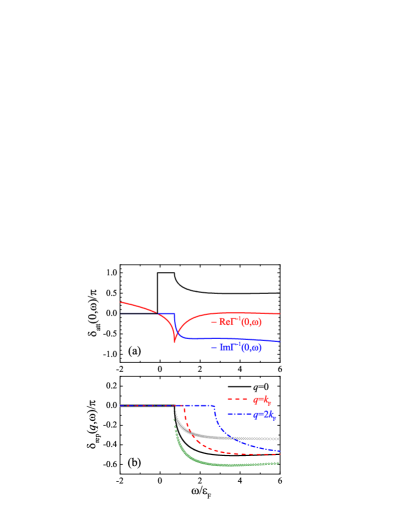
Figure 1: (Color online). (a) The in-medium phase shifts for an attractive Bose gas $\delta_{\textrm{att}}(q=0,\omega)$ at the gas parameter $na_{s}^{3}=1$. The real and imaginary parts of the negative inverse of the two-particle vertex function, $-\Gamma^{-1}(q=0,\omega)$ are also shown. (b) The corresponding in-medium phase shifts $\delta_{\textrm{rep}}(q,\omega)$ in the meta-stable upper branch at different momenta $q=0$ (black solid line), $k_{F}$ (red dashed line) and $2k_{F}$ (blue dot-dashed line). The phase shifts $\delta_{\textrm{rep}}(q=0,\omega)$ at different gas parameters $na_{s}^{3}=0.01$ and $na_{s}^{3}=-1$ are shown by gray cross and green stars, respectively. For all the plots, the temperature is fixed at $T=2T_{c0}$, where $T_{c0}\simeq 0.436T_{F}$ is the condensation temperature of an ideal Bose gas. The chemical potential $\mu$ is fixed to that of an ideal Bose gas at the same temperature, i.e., $\mu=\mu^{(0)}(2T_{c0})\simeq-0.358\varepsilon_{F}$.

II.1 In-medium phase shift for the ground state

In Fig. 1(a), we show the typical behavior of the inverse vertex function $\Gamma^{-1}$ and of the in-medium phase shift $\delta_{\textrm{att}}$ for an attractive Bose gas with the gas parameter $na_{s}^{3}=1$ at $T=2T_{c0}$, where $T_{c0}\simeq 0.436T_{F}$ is the condensation temperature of an ideal Bose gas, measured in units of Fermi temperature $T_{F}\equiv\hbar^{2}(3\pi^{2}n)^{2/3}/(2mk_{B})\equiv\varepsilon_{F}/k_{B}$. The phase shift jumps from zero to $\pi$ at the threshold frequency $\omega_{b}(\mathbf{q})$, which signals the existence of bound states. Upon increasing the frequency beyond the scattering threshold,

$$\omega_{s}\left(\mathbf{q}\right)=\frac{\hbar^{2}\mathbf{q}^{2}}{4m}-2\mu,$$ (11)

where the imaginary part of the vertex function becomes nonzero, the phase shift decreases towards $\pi/2$ as $\omega\rightarrow+\infty$. Therefore, there are two contributions to the phase shift, originating from the bound states (at $\omega_{b}(\mathbf{q})\leq\omega<\omega_{s}(\mathbf{q})$) and from the scattering states (i.e., $\omega\geq\omega_{s}(\mathbf{q})$), respectively. It is clear from Fig. 1(a) that the phase shift, as an illustrated example, does not satisfy the constraint $\delta\left(\mathbf{q},\omega=0\right)=0$. This is because we have used an artificially large chemical potential, larger than the actual chemical potential, which has to be solved self-consistently by using the number equation (10) for an attractive Bose gas.

II.2 In-medium phase shift for the upper branch

It is interesting that although we are dealing with an attractive Bose gas, we may also obtain useful information about a repulsively interacting Bose gas, by treating it as a metastable upper branch of the attractive system. This idea may be understood from the fact that there is an ambiguity in calculating the in-medium phase shift Eq. (8), as it involves a multi-valued $\ln(x)$ function. By appropriately choosing different branch cuts, one thus may access excited many-body states, in addition to the ground state of the system.

To the best of our knowledge, the proper choice of in-medium phase shift was first emphasized by Engelbrecht and Randeria in the study of a weakly interacting repulsive Fermi gas in two dimensions in 1992 Engelbrecht1992 . However, at that time, the connection between attractive and repulsive systems was not realized and the concept of the upper branch was not established. The meaning of the upper branch was only clarified in 2011 by Shenoy and Ho, who claimed that by excluding the contribution from the paired molecular states in calculating the thermodynamics of the system, one could access the upper branch of an attractive Fermi gas Shenoy2011 . This excluded molecular pole approximation (EMPA) immediately implies that for the upper branch, the lower boundary of the frequency integral in Eq. (9) should be modified to $\omega_{s}(\mathbf{q})$, leading to

$$\delta\Omega=-\frac{1}{\pi}\sum_{\mathbf{q}}\int_{\omega_{s}\left(\mathbf{q}\right)}^{+\infty}d\omega\frac{1}{e^{\beta\omega}-1}\delta_{\textrm{rep}}\left(\mathbf{q},\omega\right).$$ (12)

This expression was later applied by Li and Ho to a strongly interacting Bose gas Li2012 . However, despite the clarification of the concept of the upper branch, in those two studies (i.e., Refs. Li2012 and Shenoy2011 ), the ambiguity in the calculation of the phase shift $\delta_{\textrm{rep}}(\mathbf{q},\omega)$ was not carefully treated. The phase shift of the upper branch was directly calculated by using

$$\delta_{\textrm{rep}}^{\textrm{HO}}\left(\mathbf{q},\omega\geq\omega_{s}\left(\mathbf{q}\right)\right)=-\arctan\left[\frac{\textrm{Im$\Gamma^{-1}\left(\mathbf{q},\omega\right)$}}{\textrm{Re$\Gamma^{-1}\left(\mathbf{q},\omega\right)$}}\right]$$ (13)

without the explanation for the branch cut. Here, the function $\arctan(x)$ is the usual inverse tangent function that takes values in the first and fourth quadrant $(-\pi/2,+\pi/2)$ note1 and we have used the superscript “HO” to indicate the prescription given by Ho and co-workers.

It turns out that a more appropriate phase shift for the upper branch can be physically defined by the prescription

$$\delta_{\textrm{rep}}\left(\mathbf{q},\omega\right)=\left[\delta_{\textrm{att}}\left(\mathbf{q},\omega\right)-\pi\right]\Theta\left[\omega-\omega_{s}\left(\mathbf{q}\right)\right],$$ (14)

which can be shown from the viewpoint of the virial expansion He2015 . The $\pi$-shift in the above equation can be easily understood from the standard scattering theory: when a two-body bound state emerges, the two-particle phase shift associated with the density of states should increase by $\pi$. The prescription Eq. (14) is therefore simply the many-body generalization of the two-particle phase shift in the absence of bound states. It should be viewed as a physical realization of the EMPA approximation proposed by Ho and co-workers.

For a weakly interacting Bose gas (i.e., $a_{s}\rightarrow 0^{+}$), The two prescriptions for the upper branch phase shift, shown in Eqs. (13) and (14), agree with each other, as a result of the large value of Re$\Gamma^{-1}\left(\mathbf{q},\omega\right)$. Towards the strongly interacting limit $a_{s}\rightarrow+\infty$, however, the two prescriptions differ significantly. In particular, on the BCS side with a negative scattering length, the phase shift $\delta_{\textrm{rep}}^{\textrm{HO}}(\mathbf{q},\omega)$ coincides with the phase shift of the ground state branch, $\delta_{\textrm{att}}(\mathbf{q},\omega)$. As a result, by changing the scattering length and crossing the Feshbach resonance from below, there is a sudden branch switch from the upper branch to the ground state branch Li2012 . This branch-switching effect and the related violation of exact Tan’s relations Li2012 are absent when the more physical prescription Eq. (14) is used.

In Fig. 1(b), we show the in-medium phase shift for the upper branch, obtained by performing Eq. (14) for the attractive phase shift shown in Fig. 1(a). The Thouless criterion $\delta\left(\mathbf{q},\omega=0\right)=0$ is now strictly satisfied. Moreover, for a positive frequency the phase shift becomes negative. This leads to a positive fluctuation thermodynamic potential $\delta\Omega>0$ and a negative pair density $\delta n<0$. As analyzed by Engelbrecht and Randeria Engelbrecht1992 , the fact $\delta\Omega>0$ implies that the ground-state energy increases due to the interactions, as it should be for a repulsive system. A negative pairing density is also consistent with a repulsive interaction, which, for a specific atom, will expel other atoms away from its position, and therefore make the effective number density around its position smaller.

In Fig. 1(b), we also report the upper branch phase shift at the gas parameter $na_{s}^{3}=0.01$ (grey crosses) and $na_{s}^{3}=-1$ (green stars). It is worth noting that the negative value of the gas parameter (i.e., on the BCS side above the Feshbach resonance) actually means stronger repulsions between atoms, as indicated by the large absolute value of the phase shift. In contrast, for a positive gas parameter, the interaction effect becomes weaker with decreasing the gas parameter.

II.3 Large-$N$ expansion

The generalized NSR approach was used earlier by Li and Ho to investigate a strongly interacting Bose gas near unitarity Li2012 . A large mechanically unstable area was found when the temperature of the system is below $T<5T_{c0}\sim 2T_{F}$, which renders the approach useful only at extremely high temperatures. Here, we show that the mechanical instability is artificial and caused by the inappropriate treatment for the strong pair/density fluctuations in the NSR approach. It can be cured by the so-called large-$N$ expansion technique Nikolic2007 ; Veillette2007 ; Enss2012 .

In the large-$N$ expansion, we assign an additional flavor degree of freedom to bosonic atoms ($i,j=1,\cdots,N$) and thereby extend the model action to,

$$\mathcal{\tilde{S}} = \int d\tau d\mathbf{x}\left[\sum_{i=1}^{N}\bar{\psi_{i}}\left(\partial_{\tau}-\frac{\hbar^{2}}{2m}\nabla^{2}-\mu\right)\psi_{i}\right.$$ (15)

$$\left.+\frac{U_{0}}{2N}\sum_{i,j=1}^{N}\bar{\psi}_{i}^{2}\left(\mathbf{x},\tau\right)\psi_{j}^{2}\left(\mathbf{x},\tau\right)\right].$$

By introducing a pairing field

$$\tilde{\phi}\left(\mathbf{x},\tau\right)=\frac{U_{0}}{N}\sum_{i=1}^{N}\psi_{i}\left(\mathbf{x},\tau\right)\psi_{i}\left(\mathbf{x},\tau\right)$$ (16)

and again decoupling the interatomic interaction via the standard Hubbard-Stratonovich transformation, we integrate out the atomic fields and obtain the grand thermodynamic potential per flavor

$$\frac{\tilde{\Omega}}{N}=\Omega_{0}+\frac{1}{N}\delta\Omega+O(\frac{1}{N^{2}}),$$ (17)

up to the first non-trivial order of $O(1/N)$ Nikolic2007 ; Veillette2007 ; Enss2012 . Here, for the metastable upper branch, $\Omega_{0}$ and $\delta\Omega$ are given by Eqs. (5) and (12), respectively.

It is clear that in the large-$N$ expansion we have introduced an artificial small parameter $1/N$, which can be used to control the accuracy of the theory of strongly interacting Bose gases. The NSR approach, which is based on the summation of infinite ladder diagrams NSR1985 ; Hu2006 , should be understood as an approximate theory obtained by directly setting $N=1$. However, such a procedure cannot be justified a priori in the strongly interacting regime, as the controllable parameter $1/N$ is already at the order of unity. Indeed, the appearance of the large mechanically unstable regime at low temperatures, mentioned at the beginning of this subsection, is precisely an indication of the breakdown of the procedure of directly setting $N=1$. A more reasonable treatment is to first solve the thermodynamics of a $N$-flavor system with $N\gg 1$ and then linearly extrapolate all the desired physical quantities - as a function of $1/N$ - to the limit of $N=1$. This large-$N$ expansion idea has been successfully applied to a strongly interacting two-component Fermi gas in the unitary limit Nikolic2007 ; Veillette2007 . The equation of state and the Tan contact near the quantum critical point $\mu=0$ was then accurately predicted Enss2012 . In this work, we anticipate that the same large-$N$ expansion technique could also lead to very useful information for a unitary Bose gas in the quantum critical region.

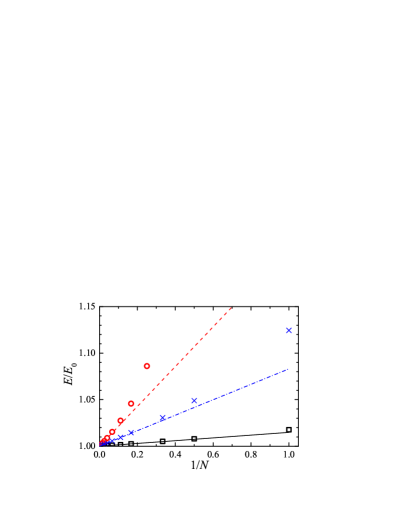
Figure 2: (Color online) Energy as a function of the artificial controlling parameter $1/N$ at $T=2T_{c0}$ (black squares for $na_{s}^{3}=10^{-6}$ and red circles for $na_{s}^{3}=1$) and $T=10T_{c0}$ (blue crosses with $na_{s}^{3}=1$). The energy is measured in units of the energy $E_{0}$ of a non-interacting Bose gas at the same temperature. The lines are linear fits to the small $1/N$ data. Note that, at low temperatures and strong interactions (i.e., red circles), we are not able to find solutions for $N=1$ because of strong correlations.

In Fig. 2, we show the $1/N$-dependence of the total energy of an interacting Bose gas at different gas parameters and temperatures, obtained by solving the coupled equations Eqs. (5), (12) and (17), and subject to the number equation $\tilde{n}/N\equiv n=n_{0}+\delta n/N$ for the number density per flavor $\tilde{n}/N$. At weak interactions (black squares) or high temperatures (blue crosses), roughly the energy changes linearly as a function of $1/N$. The linear extrapolation approximation used in the large-$N$ expansion therefore does not make significant difference. However, for a strongly interacting Bose gas at relatively low temperatures (red circles), the dependence is highly non-linear. In particular, we are not able to find physical solutions when the number of flavors $N\leq 2$. Therefore, it becomes crucial to keep only the linear term in the $1/N$ expansion, which provides the first non-trivial and non-pertrubative knowledge about a strongly correlated many-body state.

III Results and discussions

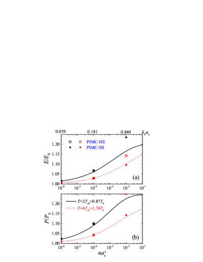
Figure 3: (Color online) The energy (a) and pressure (b) as a function of the gas parameter $na_{s}^{3}$ at $T=2T_{c0}$ (black solid lines) and $T=4T_{c0}$ (red dashed lines), normalized respectively by their corresponding results of an ideal, non-interacting Bose gas at the same temperature. The results from a path-integral Monte-Carlo calculations are also shown Pilati2006 , with squares for hard-sphere potential and circles for soft-sphere potential.

In this section, we present our large-$N$ results, calculated by the linear extrapolation towards the limit $1/N=1$. In practice, we solve the generalized NSR approach with $N=50-100$ for the chemical potential $\mu(N)$ and the energy $E(N)$, and then expand them around the corresponding non-interacting values $\mu_{0}$ and $E_{0}$,

$$\mu\left(N\right) = \mu_{0}+\delta\mu/N+O\left(1/N^{2}\right),$$ (18)

$$E\left(N\right) = E_{0}+\delta E/N+O\left(1/N^{2}\right),$$ (19)

to extract the corrections $\delta\mu$ and $\delta E$. This leads to the large-$N$ expansion results $\mu=\mu_{0}+\delta\mu$ and $E=E_{0}+\delta E$.

III.1 Crossover to strong repulsions

In Figs. 3(a) and 3(b), we present respectively the energy and pressure of an interacting Bose gas at two temperatures $T=2T_{c0}$ (black solid lines) and $T=4T_{c0}$ (red dashed lines), as a function of the gas parameter $na_{s}^{3}$, or $k_{F}a_{s}$ if we convert the number density $n$ to a Fermi wavevector $k_{F}=(3\pi^{2}n)^{1/3}$. The large-$N$ expansion results are compared with available path-integral Monte Carlo calculations for a hard-sphere (squares) and soft-sphere potential (circles) Pilati2006 . For weak interactions (i.e., $na_{s}^{3}=10^{-6}$ and $10^{-4}$ or $k_{F}a_{s}<0.2$), our predictions agree well with the ab-initio simulations. For strong interactions with strength $k_{F}a_{s}\sim 0.8$, there is a significant difference. This is due to the effect of non-negligible effective range of interactions $r_{0}$ used in the Monte Carlo simulations (i.e., $\left|k_{F}r_{0}\right|\sim 1$), which leads to a sizable correction to the energy and pressure. In our calculations with a contact interaction, the range of interactions is strictly zero.

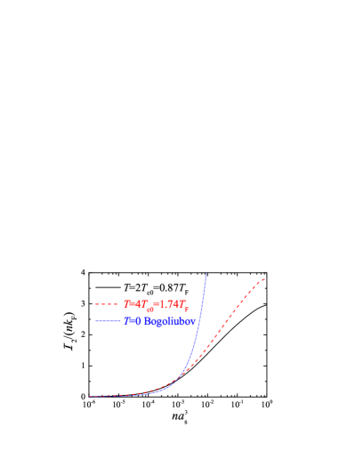
Figure 4: (Color online) Two-body contact $\mathcal{I}_{2}$ as a function of the gas parameter $na_{s}^{3}$ at $T=2T_{c0}$ (black solid line) and $T=4T_{c0}$ (red dashed line). The result from the zero-temperature Bogoliubov theory is shown by the blue dot-dashed line.

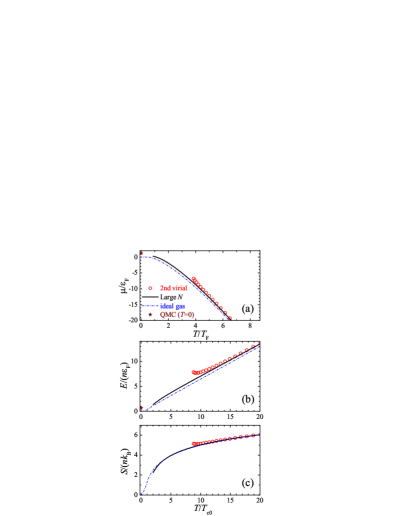
Figure 5: (Color online) Temperature dependence of the chemical potential (a), energy (b) and entropy (c) of a unitary Bose gas. For comparison, we show the second-order virial expansion predictions by red empty circles and the ideal gas results by dot-dashed lines. The latest QMC results at zero temperature are also plotted by using stars in brown Rossi2014 .

In Fig. 4, we show the evolution of the corresponding Tan’s contact with increasing gas parameter. Tan’s contact measures the density of pairs at short distance and determines the exact large-momentum or high-frequency behavior of various physical observables Tan2008 . It therefore serves as an important quantity to characterize a strongly interacting many-body system. In particular, experimentally it can be measured from the momentum distribution Makotyn2014 ; Wild2012 , which takes a $k^{-4}$ tail in the short-wavelength limit, i.e., $n(\mathbf{k})\rightarrow\mathscr{\mathcal{I}}/\mathbf{k}^{4}$. At finite temperatures, the contact can be conveniently calculated by using the adiabatic relation Tan2008 ; Hu2011NJP :

$$\mathcal{I}_{2}=-\frac{4\pi m}{\hbar^{2}}\left[\frac{\partial\Omega}{\partial a_{s}^{-1}}\right]_{T,\mu}.$$ (20)

We have used the subscript “$2$” to emphasize the fact that in our calculations we do not consider the three-body Efimov physics and the associated inelastic collisions. These effects are instead captured by a three-body contact $\mathcal{I}_{3}$, which can be defined through an adiabatic relation for a three-body parameter. We refer to Ref. Smith2014 for more detailed discussions.

The two-body contact is an increasing function of the interaction strength. At small gas parameters, our results are in good agreement with the weak-coupling predictions of a zero-temperature Bogoliubov theory (thin blue dot-dashed line) Schakel2010 ,

$$\mathcal{I}_{\textrm{bog}}=\left(4\pi na_{s}\right)^{2}\left[1+\frac{64}{3\sqrt{\pi}}\sqrt{na_{s}^{3}}\right].$$ (21)

The slight increase in our large-$N$ expansion results is due to the finite temperature effect. At large gas parameters $na_{s}^{3}$, the contact tends to saturate to a universal value that depends only on the temperature, as it should be.

III.2 Unitary Bose gases

We are now in position to discuss the universal thermodynamics of a unitary Bose gas. In Fig. 5, we present the chemical potential, energy and entropy, as a function of temperature. For comparison, we also plot in dot-dashed lines the temperature dependence of an ideal, non-interacting Bose gas. For the chemical potential and energy, our results lie systematically above the non-interacting results, clearly indicating the consequence of strong repulsions. They tends to converge to the zero temperature quantum Monte Carlo predictions (brown stars) with decreasing the temperature Rossi2014 . In contrast, the entropy seems to be less affected by strong repulsions. The insensitivity of entropy on the interatomic interactions was also previously found for a unitary Fermi gas Hu2008 ; Hu2010 ; Hu2011PRA .

At high temperatures with a small fugacity $z=e^{\beta\mu}\ll 1$, we may use the virial expansion theory to study the universal thermodynamics Liu2013 . For a unitary Bose gas, the virial expansion of the grand thermodynamic potential takes the form,

$$\Omega = \Omega_{0}-\frac{k_{B}T}{\lambda_{dB}^{3}}\left(z^{2}\Delta b_{2}+z^{3}\Delta b_{3}+\cdots\right),$$ (22)

where $\lambda_{dB}\equiv[2\pi\hbar^{2}/(mk_{B}T)]^{1/2}$ is the thermal de-Broglie wavelength, and $\Delta b_{2}=-\sqrt{2}$ is the second-order virial coefficient for strong repulsions Castin2013 ; note2 , which can be easily calculated by using Beth-Uhlenbeck formalism Beth1937 . Up to the second order, we can solve Eq. (22) together with the number equation Eq. (10). For the fugacity, we find that

$$z \simeq \sqrt{\frac{16}{9\pi}}\left(\frac{T_{F}}{T}\right)^{3/2}$$ (23)

at $T\gg T_{F}$. The virial predictions for the equation of state are shown in Fig. 5 by red circles and agree well with the large-$N$ expansion results at high temperatures.

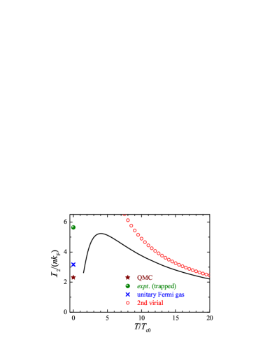
Figure 6: (Color online) Temperature dependence of the two-body contact $\mathcal{I}_{2}$ in the unitary limit. The prediction from a second-order virial expansion, Eq. (25), is shown by red empty circles. At zero temperature, the brown star and green solid circle refer to the latest QMC result Rossi2014 and the number extracted from the recent measurement at JILA for a trapped unitary Bose gas Makotyn2014 ; Smith2014 . The blue cross indicates the zero-temperature contact of a unitary Fermi gas, measured very precisely by using Bragg spectroscopy Hoinka2013 .

In the unitary limit, we may calculate the universal contact by using the adiabatic relation, Eq. (20), shown in Fig. 6. With increasing temperature, the contact initially increases and then decreases, giving rise to a peak structure at the temperature $T\sim 4T_{c0}$. The decrease of the contact at high temperatures can be well understood by using the virial expansion theory for the contact. As a direct consequence of the adiabatic relation, we have the expansion,

$$\mathcal{I}_{2} = \frac{8\pi m}{\hbar^{2}}\frac{k_{B}T}{\lambda_{dB}^{2}}\left(z^{2}c_{2}+z^{3}c_{3}+\cdots\right),$$ (24)

where $c_{n}=\lambda_{dB}^{-1}(\partial\Delta b_{n}/\partial a_{s}^{-1})$ is the so-called contact coefficient Hu2011NJP . For a unitary Bose gas, by using Beth-Uhlenbeck formalism it is easy to show that $c_{2}=2/\pi$. Using Eq. (23), we then find

$$\frac{I_{2}}{nk_{F}} \simeq \frac{64}{3}\left(\frac{T_{F}}{T}\right).$$ (25)

Thus, at high temperatures the contact decreases as $T^{-1}$. There is no apparent physical explanation for the increase of the contact at low temperatures. However, we notice that with decreasing temperature toward zero temperature, our large-$N$ expansion result seems to be consistent with the zero-temperature value predicted by the latest quantum Monte Carlo simulation Rossi2014 .

For comparison, we show the experimental data of the contact Makotyn2014 , analyzed by Smith and co-workers (green solid circle) Smith2014 . The significant discrepancy between experiment and our large-$N$ theory should be largely due to the unknown temperature in the experiment, as the Bose cloud could be significantly heated by atom losses Makotyn2014 . We also show the zero-temperature contact of a unitary Fermi gas (blue cross), which has been both calculated and measured very accurately Hoinka2013 . It is interesting that both the unitary Bose and Fermi gases have similar contact at zero temperature, indicating that a 3D Bose gas may also have the tendency of being fermionized at strong repulsions, analogous to a Bose gas in one dimension.

IV Conclusions

In summary, based on the upper branch idea and large-$N$ expansion technique, we have developed a unified theory for a normal, strongly interacting Bose gas. The theory reproduces the path-integral Monte Carlo simulation in the weak-coupling limit Rossi2014 . While at high temperatures, it nicely recovers the known results from a quantum virial expansion calculation Castin2013 ; Liu2013 . Thus, we anticipate that the universal thermodynamics predicted by our theory could be qualitatively reliable. A useful check may be provided by experimentally measuring the finite-temperature contact of a unitary Bose gas through momentum distribution or momentum-resolved radio-frequency spectroscopy Makotyn2014 .

Our results complement the earlier studies of a condensed strongly interacting Bose gas. It is worth nothing that our theoretical framework can naturally be extended to include the condensation (i.e., $T<T_{c0}$) by using a generalized Nozières-Schmitt-Rink approach below the superfluid transition temperature Hu2006 . This extension will be addressed in a future investigation.

- (1) A. Griffin, T. Nikuni, and E. Zaremba, Bose-Condensed Gases at Finite Temperatures (Cambridge University Press, Cambridge, UK, 2009).
- (2) A. Griffin, Phys. Rev. B 53, 9341 (1996).
- (3) H. Shi and A. Griffin, Phys. Rep. 304, 1 (1998).
- (4) X.-J. Liu, H. Hu, A. Minguzzi, and M. P. Tosi, Phys. Rev. A 69, 043605 (2004).
- (5) T. Kita, Phys. Rev. B 80, 214502 (2009).
- (6) F. Cooper, C.-C. Chien, B. Mihaila, J. F. Dawson, and E. Timmermans, Phys. Rev. Lett. 105, 240402 (2010).
- (7) F. Cooper, B. Mihaila, J. F. Dawson, C.-C. Chien, and E. Timmermans, Phys. Rev. A 83, 053622 (2011).
- (8) Y.-H. Zhang and D. Li, Phys. Rev. A 88, 053604 (2013).
- (9) V. I. Yukalov and E. P. Yukalova, Phys. Rev. A 90, 013627 (2014).
- (10) T. D. Lee and C. N. Yang, Phys. Rev. 105, 1119 (1957).
- (11) T. D. Lee, K. Huang, and C. N. Yang, Phys. Rev. 106, 1135 (1957).
- (12) S. T. Beliaev, Sov. Phys. JETP 7, 289 (1958); 7, 299 (1958).
- (13) N. N. Bogoliubov, J. Phys. (USSR) 11, 23 (1947).
- (14) I. Bloch, J. Dalibard, and W. Zwerger, Rev. Mod. Phys. 80, 885 (2008).
- (15) P. O. Fedichev, M. W. Reynolds, and G. V. Shlyapnikov, Phys. Rev. Lett. 77, 2921 (1996).
- (16) T. Weber, J. Herbig, M. Mark, H.-C. Nägerl, and R. Grimm, Phys. Rev. Lett. 91, 123201 (2003).
- (17) V. Efimov, Phys. Lett. 33B, 563 (1970).
- (18) S. B. Papp, J. M. Pino, R. J. Wild, S. Ronen, C. E. Wieman, D. S. Jin, and E. A. Cornell, Phys. Rev. Lett. 101, 135301 (2008).
- (19) N. Navon, S. Piatecki, K. Günter, B. S. Rem, T. C. Nguyen, F. Chevy, W. Krauth, and C. Salomon, Phys. Rev. Lett. 107, 135301 (2011).
- (20) B. S. Rem, A. T. Grier, I. Ferrier-Barbut, U. Eismann, T. Langen, N. Navon, L. Khaykovich, F. Werner, D. S. Petrov, F. Chevy, and C. Salomon, Phys. Rev. Lett. 110, 163202 (2013).
- (21) R. J. Fletcher, A. L. Gaunt, N. Navon, R. P. Smith, and Z. Hadzibabic, Phys. Rev. Lett. 111, 125303 (2013).
- (22) P. Makotyn, C. E. Klauss, D. L. Goldberger, E. A. Cornell, and D. S. Jin, Nature Phys. 10, 116 (2014).
- (23) J. P. D’Incao, H. Suno, and B. D. Esry, Phys. Rev. Lett. 93, 123201 (2004).
- (24) S. Cowell. H. Heiselberg, I. E. Mazets, J. Morales, V. R. Pandharipande, and C. J. Pethick, Phys. Rev. Lett. 88, 210403 (2002).
- (25) J.-L. Song and F. Zhou, Phys. Rev. Lett. 103, 025302 (2009).
- (26) Y.-L. Lee and Y.-W. Lee, Phys. Rev. A 81, 063613 (2010).
- (27) J. M. Diederix, T. C. F. van Heijst, and H. T. C. Stoof, Phys. Rev. A 84, 033618 (2011).
- (28) D. Borzov, M. S. Mashayekhi, S. Zhang, J.-L. Song, and F. Zhou, Phys. Rev. A 85, 023620 (2012).
- (29) W. Li and T.-L. Ho, Phys. Rev. Lett. 108, 195301 (2012).
- (30) X. Yin and L. Radzihovsky, Phys. Rev. A 88, 063611 (2013).
- (31) S. Piatecki and W. Krauth, Nat. Commun. 5, 3503 (2014).
- (32) D. H. Smith, E. Braaten, D. Kang, and L. Platter, Phys. Rev. Lett. 112, 110402 (2014).
- (33) A. G. Skyes, J. P. Corson, J. P. D’Incao, A. P. Koller, C. H. Greene, A. M. Rey, K. R. A. Hazzard, and J. L. Bohn, Phys. Rev. A 89, 021601(R) (2014).
- (34) S.-J. Jiang, W.-M. Liu, G. W. Semenoff, and F. Zhou, Phys. Rev. A 89, 033614 (2014).
- (35) M. Rossi, L. Salasnich, F. Ancilotto, and F. Toigo, Phys. Rev. A 89, 041602(R) (2014).
- (36) S. Laurent, X. Leyronas, and F. Chevy, Phys. Rev. Lett. 113, 220601 (2014).
- (37) M. Rossi, F. Ancilotto, L. Salasnich, and F. Toigo, arXiv:1408.3945 (2014).
- (38) F. Ancilotto, M. Rossi, L. Salasnich, and F. Toigo, arXiv:1501.0549 (2015).
- (39) L. He, X.-J. Liu, X.-G. Huang, and H. Hu, arXiv:1412.2412 (2014).
- (40) P. Nikolić and S. Sachdev, Phys. Rev. A 75, 033608 (2007).
- (41) M. Y. Veillette, D. E. Sheehy, and L. Radzihovsky, Phys. Rev. A 75, 043614 (2007).
- (42) T. Enss, Phys. Rev. A 86, 013616 (2012).
- (43) S. Pilati, K. Sakkos, J. Boronat, J. Casulleras, and S. Giorgini, Phys. Rev. A 74, 043621 (2006).
- (44) X.-J. Liu, H. Hu, and P. D. Drummond, Phys. Rev. Lett. 102, 160401 (2009).
- (45) X.-J. Liu, H. Hu, and P. D. Drummond, Phys. Rev. A 82, 023619 (2010).
- (46) X.-J. Liu, H. Hu, and P. D. Drummond, Phys. Rev. B 82, 054524 (2010).
- (47) Y. Castin and F. Werner, Canadian Journal of Physics 91, 382 (2013).
- (48) X.-J. Liu, Phys. Rep. 524, 37 (2013).
- (49) S. Tan, Ann. Phys. (NY) 323, 2952 (2008); 323, 2971 (2008).
- (50) V. N. Popov, Functional Integrals and Collective Excitations (Cambridge University Press, Cambridge, UK, 1987).
- (51) A. Koetsier, P. Massignan, R. A. Duine, and H. T. C. Stoof, Phys. Rev. A 79, 063609 (2009).
- (52) D. M. Eagles, Phys. Rev. 186, 456 (1969).
- (53) A. J. Leggett, Modern Trends in the Theory of Condensed Matter (Springer-Verlag, Berlin, 1980), pp. 13-27.
- (54) P. Nozières and S. Schmitt-Rink, J. Low Temp. Phys. 59, 195 (1985).
- (55) C. A. R. Sá de Melo, M. Randeria, and J. R. Engelbrecht, Phys. Rev. Lett. 71, 3202 (1993).
- (56) H. Hu, X.-J. Liu, and P. D. Drummond, Europhys. Lett. 74, 574 (2006).
- (57) J. R. Engelbrecht and M. Randeria, Phys. Rev. B 45, 12419 (1992).
- (58) V. B. Shenoy and T.-L. Ho, Phys. Rev. Lett. 107, 210401 (2011).
- (59) We refer to the Appendix of Ref. He2015 for a detailed discussion.
- (60) R. J. Wild, P. Makotyn, J. M. Pino, E. A. Cornell, and D. S. Jin Phys. Rev. Lett. 108, 145305 (2012).
- (61) H. Hu, X.-J. Liu, and P. D. Drummond, New J. Phys. 13, 035007 (2011).
- (62) A.M.J. Schakel, arXiv:1007.3452 (2010).
- (63) H. Hu, X.-J. Liu, and P. D. Drummond, Phys. Rev. A 77, 061605(R) (2008).
- (64) H. Hu, X.-J. Liu, and P. D. Drummond, New J. Phys. 12, 063038 (2010).
- (65) H. Hu, X.-J. Liu, and P. D. Drummond, Phys. Rev. A 83, 063610 (2011).
- (66) It is easy to show that, in the unitary limit, the second-order virial coefficients for an attractive and repulsive gas differ by a minus sign.
- (67) E. Beth and G. E. Uhlenbeck, Physica 4, 915 (1937).
- (68) S. Hoinka, M. Lingham, K. Fenech, H. Hu, C. J. Vale, J. E. Drut, and S. Gandolfi, Phys. Rev. Lett. 110, 055305 (2013).