Feedback stabilization for the mass balance equations of a food extrusion process

Abstract

In this paper, we study the stabilization problem for a food extrusion process in the isothermal case. The model expresses the mass conservation in the extruder chamber and consists of a hyperbolic Partial Differential Equation (PDE) and a nonlinear Ordinary Differential Equation (ODE) whose dynamics describes the evolution of a moving interface. By using a Lyapunov approach, we obtain the exponential stabilization for the closed-loop system under natural feedback controls through indirect measurements.

I Introduction

Screw extruders have become very popular for their ability to manufacture food and plastics products with desired shapes and properties. Due to the strong interaction between the mass, the energy and the momentum balances occurring in those processes, the design of efficient controllers still remains a hard task at the industrial level. So far, the control oriented model of extruders are issued from some black box model of limited operational validity. Following the objectives of the control, these models describes the extruder’s temperature and flow rate at the die output or the pressure dynamics based on single input and single output or multiple input and multiple output system. Generally, extrusion processes are controlled using PID [13, 18, 10] or predictive controllers [20, 9] with oversimplified or empirical models. In [13], the volumetric expansion of the extrudate correlated to the die temperature and pressure and the specific mechanical energy is chosen as the key product quality to be controlled. The authors study the performance of the PI controller based on the regulation of the die pressure using feed rate as a manipulative variable and show that the response of an improperly tuned controller may be too sluggish on one hand, or too oscillatory on the other hand. First-order, second-order and Lead-lag Laplace transfer-function are exploited in [19] to design a feedforward controller for a twin-screw food extrusion process to reduce the effect of feed rate and feed moisture content variations on the die pressure. The experimental results showed that the die pressure response varies with the operation conditions, so a single gain value would not be suitable for all operating conditions. The complexity of the process suggests adaptive control methods because of the frequent changes occurring during the extruder operation in the feed composition [19]. [17] uses second-order transfer functions while emphasizing the difficulty in implementing those types of model-based controllers due to the strong influence of all the manipulated inputs and measurable process variables. Therefore, very intelligent controllers need to be constructed for extrusion cooking process based on a control algorithm developed from process experience. We mention that the transport delays, the strong interactions and the non-linearities make it difficult to control such systems with PID controllers. Predictive controllers might offer better performances but are somewhat difficult to implement [21].

In the present work, we consider the stabilization of the die pressure to the desired setpoint in a food extrusion process. The controller is constructed based on a bi-zone model derived from the computation of the conservation of mass in the extruder under the assumption of constant temperature and viscosity. A Geometric decomposition of the extruder length in Partially Filled Zone (PFZ) and Fully Filled Zone (FFZ) allows to describe the process by a transport equation and a pressure-gradient equation defined on complementary time varying spatial domains. The domains are coupled by a moving interface whose dynamics is governed by an ODE representing the total mass balance in an extruder. We emphasize that an accurate die pressure regulation is critical to ensure the uniformity of the extruded melt and is strongly related to the quality of the final product. We propose a suitable feedback control laws together with practical measurements as output such that the solution of the closed-loop system converges to a desired steady-state or equilibrium asymptotically.

The stabilization problems for hyperbolic systems has been widely studied in the literature. The first approach relies on careful analysis of the classical solutions along the characteristics. We refer to Greenberg and Li [11] in the case of second-order system of conservation laws and more general situations on $n$th-order systems by Li in [16].

Another approach based on Lyapunov techniques was introduced by Coron et al. in [4]. This approach was improved by in [3] where a strict Lyapunov function in terms of Riemann invariants was constructed and its time derivative can be made negative definite by choosing properly the boundary conditions. The Lyapunov function is very useful to analyze nonlinear hyperbolic systems of conservation laws because of its rubustness, see [1, 2, 6, 3, 5, 23, 22] for a wide range of applications to various models. Among which, we are interested in a physical model for the extrusion process which occurs very often in polymer material and food production.

The main contribution of this paper is to establish the exponential stabilization for the extrusion model under natural feedbacks by a Lyapunov function approach motivated by [3, 5, 23]. The difficulties come from three aspects: 1) The domains on which the conservation laws are defined depend on the solution through the dynamical interface; 2) The nonlinear coupling of the dynamics of the interface and the filling ratio in the Partially Filled Zone (PFZ) is not standard; 3) The measurements and the feedbacks are natural, however, some of the measurements are indirect, i.e., the measurements are not a part of solution but given through a indirect relation of solution.

The organization of the paper is as follows. In Section II, we give the physical description of the model. The main result on stabilization (Theorem 1) and its proof are given in Section III. Numerical simulations are provided in Section IV. Finally in Section V, we give our conclusion and some perspectives in control of the extrusion process.

II Description of the model

An extruder is a process used for manufacturing objects with fixed shapes and specific properties, see Fig. 1. One or two Archimedean screws are rotating inside the barrel in order to convect the extruded material from the feed to the die exit. In food or polymers extrusion processes, the ultimate control systems involved manipulation of screw speed, feed rate, inlet solvent fraction, and barrel temperature for the regulation of moisture content, temperature and viscosity of the finite product, residence time and die flow, etc.

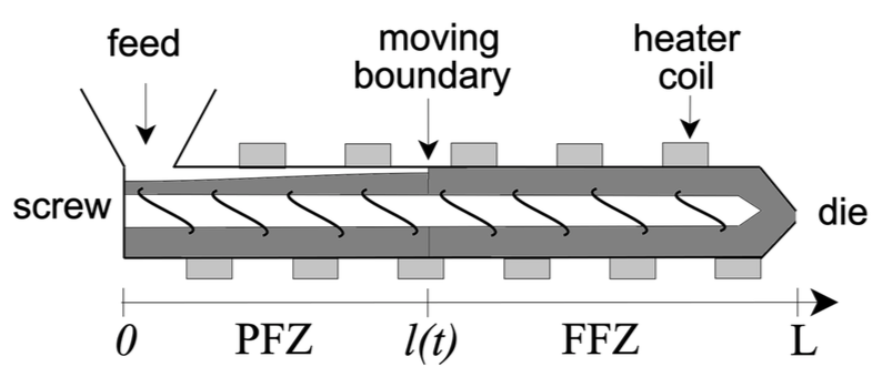
Figure 1: A single-screw screw extruder

In this paper, we consider the mass balances model [7, 8] motivated by [14, 15] for cooking extrusion process. In this case, the material convection along the extruder chamber of length $L$ is described in two zones: the PFZ ($[0,l(t)]$ in space) and a FFZ ($[l(t),L]$ in space) separated by a moving interface $l(t)$. The PFZ and the FFZ appear due to the die resistance that provokes an accumulation phenomena and high pressure need to be built-up to evict the extrudate out of the die. By the mass conservation principle the convection in the PFZ is described by the evolution of the filling ratio $f_{p}(t,x)$ for an homogeneous melt. The melt convection speed in the PFZ, namely, $\alpha_{p}$ depends on the screw speed $N(t)$ whereas the FFZ transport velocity is related to the die pressure $P(t,L)$: $\alpha_{p}\neq\alpha_{f}$. Under the assumption of constant viscosity $\eta$ along the extruder, the dynamics of the moving interface $l(t)$ is governed by an ODE arising from the difference of the convection speed in the two regions. The flow rate in the FFZ is constant and equal to the die flow rate $F_{d}(t)$ which is proportional to the pressure difference $\Delta P(t):=P(t,L)-P_{0}$ where $P_{0}$ denotes the atmospheric pressure. For more detailed physical description of the model and definition of all the parameters appeared below, one can refer to [7, 8].

In this work, the stabilization of $(l(t),f_{p}(t,x))$ with the help of the actuated screw speed $N(t)$ and inlet flow rate $F_{in}(t)$ is established based on feedbacks that depend on the pressure difference $\Delta P(t)$ that is a practically useful measurement for the system. Considering the following change of variables

$$x\mapsto y=\frac{x}{l(t)}\ \text{in \emph{PFZ}}\ \text{and}\ x\mapsto y=\frac{x-l(t)}{L-l(t)}\ \text{in \emph{FFZ}},$$ (1)

respectively, the time varying domains ($[0,l(t)]$, $[l(t),L]$) can be transformed to the fixed domain $[0,1]$ in space. For the sake of simplicity, we still denote by $x$ the space variable instead of $y$. More precisely, we consider the stabilization problem for the corresponding normalized system on the spatial domain $[0,1]$. The interface dynamics which arises from a total mass balance writes

$$\begin{cases}\dot{l}(t)=\mathcal{F}(l(t),N(t),f_{p}(t,1)),\quad&\text{in}\ \mathbb{R}^{+}=(0,\infty),\\ l(0)=l^{0},\end{cases}$$ (2)

where

$$\mathcal{F}(l(t),N(t),f_{p}(t,1))=\frac{\frac{K_{d}}{\eta}\Delta P(t)-\rho_{o}V_{eff}N(t)f_{p}(t,1)}{\rho_{o}S_{eff}(1-f_{p}(t,1))},$$ (3)

$K_{d}$ , $\rho_{0}$, $\eta$ denote the die conductance, the melt density and the viscosity, respectively. $V_{eff}$ and $S_{eff}$ are the effective volume and section between a screw element and the extruder barrel, respectively. Assuming a constant viscosity along the extruder (the isothermal case), the relation

$$\Delta P(t)=\mathcal{P}(N(t),l(t)):=\frac{\eta\rho_{o}V_{eff}N(t)(L-l(t))}{B\rho_{o}+K_{d}(L-l(t))}$$ (4)

is determined by integrating the pressure-gradient equation corresponding to the momentum balance in the FFZ and considering a pressure continuity coupling relation at the normalized interface, namely, $P(0,t)=P_{0}$ in the PFZ [8]. The filling ratio in the PFZ writes

$$\begin{cases}\partial_{t}f_{p}(t,x)+\alpha_{p}\partial_{x}f_{p}(t,x)=0,\quad&\text{in}\ \mathbb{R}^{+}\times(0,1),\\ f_{p}(0,x)=f^{0}_{p}(x),\quad&\text{in}\ (0,1),\\ f_{p}(t,0)=\frac{F_{in}(t)}{\rho_{o}V_{eff}N(t)},\quad&\text{in}\ \mathbb{R}^{+},\end{cases}$$ (5)

where

$$\alpha_{p}=\frac{\zeta N(t)-x\mathcal{F}(l(t),N(t),f_{p}(t,1))}{l(t)}.$$ (6)

III Main result and its proof

Let us define the constant equilibrium $l_{e}\in(0,L)$, $f_{p_{e}}\in(0,1)$, $N_{e}$, $\Delta P_{e}$, $\alpha_{p_{e}}$ and $F_{in_{e}}$ by $F(l_{e},N_{e},f_{p_{e}})=0$, $\Delta P_{e}=\mathcal{P}(l_{e},N_{e})$, $\alpha_{p_{e}}=\frac{\zeta N_{e}}{l_{e}}$, $F_{in_{e}}=\rho_{o}V_{eff}N_{e}f_{p_{e}}$. Denote the difference $\bar{l}(t):=l(t)-l_{e},\bar{N}(t):=N(t)-N_{e},\bar{f}_{p}(t,x):=f_{p}(t,x)-f_{p_{e}},\bar{F}_{in}(t):=F_{in}(t)-F_{in_{e}},\Delta\bar{P}(t):=\Delta P(t)-\Delta P_{e}$ and the constants

$$\begin{cases}(a_{1},a_{2},a_{3})=\Big{(}\frac{\partial F}{\partial l},\frac{\partial F}{\partial N},\frac{\partial F}{\partial f_{p}}\Big{)}\Big{|}_{(l_{e},N_{e},f_{p_{e}})},\\ (b_{1},b_{2})=\Big{(}\frac{\partial\mathcal{P}}{\partial l},\frac{\partial\mathcal{P}}{\partial N}\Big{)}\Big{|}_{(l_{e},N_{e})}.\end{cases}$$ (7)

The linear feedback law that we use is the following one:

$$\bar{N}(t)=k_{1}\cdot\Delta\bar{P}(t),\quad\bar{F}_{in}(t)=k_{2}\cdot\Delta\bar{P}(t),$$ (8)

where $\Delta P(t)$, thus $\Delta\bar{P}(t)$, is measurable. The aim of stabilization is to find constants $k_{1},k_{2}\in\mathbb{R}$ such that the closed-loop system (2) and (5) with feedback (8) is asymptotically stable, i.e., $(\bar{l}(t),\bar{f}_{p}(t,\cdot))\rightarrow 0$ as $t\rightarrow\infty$.

Concerning the well-posedness of the Cauchy problem (2) and (5) with feedback (8), we have the following proposition.

Proposition 1.

Let $k_{1},k_{2}\in\mathbb{R}$ be fixed. There exists $\varepsilon>0$ such that for any $l^{0}\in\mathbb{R}$, $f^{0}_{p}\in H^{2}(0,1)$ satisfying $|l^{0}-l_{e}|^{2}+\|f^{0}_{p}(\cdot)-f_{p_{e}}\|^{2}_{H^{2}(0,1)}\leqslant\varepsilon$, and the compatibility conditions at the point $(t,x)=(0,0)$, system (2) and (5) with (8) has a unique solution $(l,f_{p})\in W^{1,\infty}([0,T))\times C^{0}([0,T);H^{2}(0,1))$ for some $T\in(0,\infty]$. Moreover, if $|l(t)-l_{e}|^{2}+\|f_{p}(t,\cdot)-f_{p_{e}}\|^{2}_{H^{2}(0,1)}\leqslant\varepsilon$ for all $t\in[0,T),$ then $T=\infty$.

Remark 1.

The compatibility conditions at the point $(t,x)=(0,0)$ are the following:

$$f_{p}^{0}(0)=\frac{F_{in}(0)}{\rho_{o}V_{eff}N(0)};$$ (9)

$$\frac{\dot{F}_{in}(0)N(0)-F_{in}(0)\dot{N}(0)}{\rho_{o}V_{eff}N(0)}+\frac{\zeta N(0)}{l^{0}}f_{p}^{0^{\prime}}(0)=0,$$ (10)

where $N(0),F_{in}(0)$ are determined by (4), (8) with $l(0)=l^{0}$, while $\dot{N}(0)$, $\dot{F}_{in}(0)$ are determined by differentiating (4) and (8) together with $\dot{l}(0)=F(l^{0},N(0),f_{p}^{0}(1))$.

The proof of Proposition 1 is based on fixed point argument and one can refer to [8] for the well-posedness of the corresponding open-loop system. Our main result on stabilization of the interface position $l(t)$ and the filling ratio $f_{p}(t,x)$ is the following theorem.

Theorem 1.

Suppose that there exist $k_{1},k_{2}\in\mathbb{R}$ such that

$$a_{1}+\frac{k_{1}a_{2}b_{1}}{1-k_{1}b_{2}}<0,$$ (11)

$$\left|\frac{a_{3}b_{1}(k_{2}-f_{p_{e}}\rho_{o}V_{eff}k_{1})}{\rho_{o}V_{eff}N_{e}(1-k_{1}b_{2})}\right|<\left|a_{1}+\frac{k_{1}a_{2}b_{1}}{1-k_{1}b_{2}}\right|,$$ (12)

where $a_{1},a_{2},a_{3},b_{1},b_{2}$ are given in (7). Then, the nonlinear system (2) and (5) is locally exponentially stable under the feedback (8), i.e., there exist constants $\varepsilon>0$, $M>0$ and $\omega>0$ such that for any $l^{0}\in\mathbb{R}$, $f^{0}_{p}\in H^{2}(0,1)$ satisfying

$$|l^{0}-l_{e}|^{2}+\|f^{0}_{p}(\cdot)-f_{p_{e}}\|^{2}_{H^{2}(0,1)}\leqslant\varepsilon,$$ (13)

and the compatibility conditions at the point $(t,x)=(0,0)$, the solution of (2) and (5) with (8) satisfies

$$|l(t)-l_{e}|^{2}+\|f_{p}(t,\cdot)-f_{p_{e}}\|^{2}_{H^{2}(0,1)}$$

$$\leqslant Me^{-\omega t}\Big{(}|l^{0}-l_{e}|^{2}+\|f^{0}_{p}(\cdot)-f_{p_{e}}\|^{2}_{H^{2}(0,1)}\Big{)},\quad\forall t\geqslant 0.$$ (14)

Before the proof of Theorem 1, we give several remarks.

Remark 2.

The existence of $k_{1},k_{2}\in\mathbb{R}$ satisfying (11)-(12) depends on $a_{1},a_{2},a_{3},b_{1},b_{2}$, see Proposition 2 below. Its proof is given in Appendix.

Proposition 2.

There exist $k_{1},k_{2}\in\mathbb{R}$ such that (11)-(12) hold if and only if either 1) $a_{1}<0$; or 2) $a_{1}\geqslant 0$ and $a_{2}b_{1}\neq 0$.

Remark 3.

The measurement on $\Delta P(t)$ is of practical reason, thus the feedback (8) is indirect in the sense that the measurements are made not on the solution $(l(t),f_{p}(t,x))$ itself.

Remark 4.

The proof of Theorem 1 relies on a Lyapunov function approach. The weight as $e^{-\gamma_{i}x}$ is essential to get a strict Lyapunov function. One can refer to the stabilization results by such weighted Lyapunov functions, for quite general linear hyperbolic systems in [23, 22]; for one dimensional Euler equation with variable coefficients in [12]; for a conservation law with nonlocal velocity in [5].

Proof of Theorem 1: The construction of the Lyapunov functions is divided into three steps.

Step 1. The stabilization of $l(t)$ and $f_{p}(t,\cdot)$ in $L^{2}(0,1)$.

Let

$$V_{0}(t)=\bar{l}^{2}(t),\quad V_{1}(t)=\int_{0}^{1}e^{-\gamma_{1}x}\bar{f}^{2}_{p}(t,x)\,dx,$$ (15)

where $\gamma_{1}>0$ is a constant to be chosen later.

Lemma 1.

There exist positive constants $A_{1},\gamma_{1},\beta_{0},\beta_{1},\delta_{1}$ such that the following estimates hold for every solution to system (2) and (5) with (8)

$$\dot{V}_{0}(t)+A_{1}\dot{V}_{1}(t)\leqslant -(\beta_{0}+o(1))V_{0}(t)-(\beta_{1}+o(1))V_{1}(t)$$

$$-(\delta_{1}+o(1))\bar{f}_{p}^{2}(t,1),$$ (16)

where $o(1)$ represents various terms which tend to $0$ when $|(\bar{l}(t),\bar{N}(t),\bar{f}_{p}(t,1))|\rightarrow 0.$

Proof of Lemma 1: By definition of the equilibrium $(l_{e},N_{e},f_{p_{e}})$ and the constants $(a_{1},a_{2},a_{3},b_{1},b_{2})$, it is easy to get by expansion that

$$\mathcal{F}(l(t),N(t),f_{p}(t,1))=(a_{1}+o(1))\,\bar{l}(t)+(a_{2}+o(1))\,\bar{N}(t)$$

$$\hskip 102.42992pt+(a_{3}+o(1))\,\bar{f}_{p}(t,1),$$ (17)

$$\Delta\bar{P}(t)=(b_{1}+o(1))\,\bar{l}(t)+(b_{2}+o(1))\,\bar{N}(t).$$ (18)

Furthermore, it follows from (8) and (18) that

$$\Delta\bar{P}= \Big{(}\frac{b_{1}}{1-k_{1}b_{2}}+o(1)\Big{)}\bar{l}(t),$$ (19)

$$\bar{N}(t)= \Big{(}\frac{k_{1}b_{1}}{1-k_{1}b_{2}}+o(1)\Big{)}\bar{l}(t),$$ (20)

$$\bar{F}_{in}(t)= \Big{(}\frac{k_{2}b_{1}}{1-k_{1}b_{2}}+o(1)\Big{)}\bar{l}(t).$$ (21)

Differentiating $V_{0}(t)$ with respect to $t$ and using (2), (III) and (20), one easily gets that

$$\dot{V}_{0}(t)= 2\bar{l}(t)\cdot\mathcal{F}(l(t),N(t),f_{p}(t,1))$$

$$= (2\theta_{0}+o(1))\bar{l}^{2}(t)+(2a_{3}+o(1))\bar{l}(t)\bar{f}_{p}(t,1).$$ (22)

where $\theta_{0}=a_{1}+\displaystyle\frac{k_{1}a_{2}b_{1}}{1-k_{1}b_{2}}<0.$

On the other hand, (6) and (III) yield that

$$\alpha_{p}=\alpha_{p_{e}}+o(1),\quad\alpha_{p_{x}}=o(1).$$ (23)

Differentiating $V_{1}(t)$ gives, from (15), (23), (23) and integration by parts, that

$$\dot{V}_{1}(t)= BT_{1}+\int_{0}^{1}(-\gamma_{1}\alpha_{p}+\alpha_{p_{x}})e^{-\gamma_{1}x}\bar{f}^{2}_{p}(t,x)\,dx$$

$$= BT_{1}-(\gamma_{1}\alpha_{p_{e}}+o(1))V_{1}(t),$$ (24)

where

$$BT_{1}=-e^{-\gamma_{1}}(\alpha_{p_{e}}+o(1))\bar{f}^{2}_{p}(t,1)+(\alpha_{p_{e}}+o(1))\bar{f}^{2}_{p}(t,0).$$ (25)

Note that by (5),(20)-(21), we have

$$\bar{f}_{p}(t,0)=\frac{F_{in}(t)}{\rho_{o}V_{eff}N(t)}-f_{p_{e}}=(\theta_{1}+o(1))\bar{l}(t),$$ (26)

where $\theta_{1}=\frac{b_{1}(k_{2}-f_{p_{e}}\rho_{o}V_{eff}k_{1})}{\rho_{o}V_{eff}N_{e}(1-k_{1}b_{2})}$. Combining (23), (III), (25), (26), we get consequently

$$\dot{V}_{1}(t)= -(\gamma_{1}\alpha_{p_{e}}+o(1))V_{1}(t)-(e^{-\gamma_{1}}\alpha_{p_{e}}+o(1))\bar{f}^{2}_{p}(t,1)$$

$$+(\alpha_{p_{e}}\theta_{1}^{2}+o(1))V_{0}(t).$$ (27)

Under the assumption of (11)-(12), it is easy to get the existence of $A_{1}>0$ and $\gamma_{1}>0$ (suitably small) such that

$$\left(\begin{matrix}2\theta_{0}+A_{1}\alpha_{p_{e}}\theta_{1}^{2}&a_{3}\\ a_{3}&-A_{1}e^{-\gamma_{1}}\alpha_{p_{e}}\\ \end{matrix}\right)$$ (28)

is negative definite. This concludes the proof of Lemma 1 with (III) and (III). ∎

Step 2. The stabilization of $f_{p_{x}}(t,\cdot)$ in $L^{2}(0,1)$.

Differentiating (5) with respect to $x$, we get

$$\begin{cases}f_{p_{xt}}+\alpha_{p}f_{p_{xx}}+\alpha_{p_{x}}f_{p_{x}}=0,\\ f_{p_{x}}(0,x)=f^{0^{\prime}}_{p}(x),\\ f_{p_{x}}(t,0)=\displaystyle\frac{-f_{p_{t}}(t,0)}{\alpha_{p}|_{x=0}},\end{cases}$$ (29)

where

$$f_{p_{t}}(t,0)=\frac{\dot{F}_{in}(t)N(t)-F_{in}(t)\dot{N}(t)}{\rho_{o}V_{eff}N^{2}(t)}.$$ (30)

Let

$$V_{2}(t)=\int_{0}^{1}e^{-\gamma_{2}x}f^{2}_{p_{x}}(t,x)\,dx,$$ (31)

where $\gamma_{2}>0$ is a constant.

Lemma 2.

There exist positive constants $\gamma_{2},\beta_{2},\delta_{2},\theta_{2}$ such that the following estimate holds for every solution to system (2) and (5) with (8)

$$\dot{V}_{2}(t)\leqslant -(\beta_{2}+o(1))V_{2}(t)-(\delta_{2}+o(1))f_{p_{x}}^{2}(t,1)$$

$$+\theta_{2}(V_{0}(t)+\bar{f}_{p}^{2}(t,1)).$$ (32)

Proof of Lemma 2. Differentiating (4) and (8) with respect to $t$ gives that,

$$\begin{cases}\dot{N}(t)=k_{1}\cdot\Delta\dot{P}(t),\quad\dot{F}_{in}(t)=k_{2}\cdot\Delta\dot{P}(t),\\ \small\Delta\dot{P}(t)=\frac{\partial\mathcal{P}}{\partial l}\big{|}_{(l(t),N(t))}\dot{l}(t)+\frac{\partial\mathcal{P}}{\partial N}\big{|}_{(l(t),N(t))}\dot{N}(t).\end{cases}$$ (33)

Then it follows from (2), (7), (III), (19) and (33) that

$$\Delta\dot{P}(t)= \frac{\frac{\partial\mathcal{P}}{\partial l}\big{|}_{(l(t),N(t))}}{1-k_{1}\frac{\partial\mathcal{P}}{\partial N}\big{|}_{(l(t),N(t))}}\cdot\dot{l}(t)$$

$$= O(1)(\bar{l}(t)+\bar{N}(t)+\bar{f}_{p}(t,1)),$$ (34)

where $O(1)$ denotes various terms which are uniformly bounded when $|(\bar{l}(t),\bar{N}(t),\bar{f}_{p}(t,1))|\rightarrow 0$.

Combining (20), (29)-(30) and (33)-(III), we get easily that

$$f_{p_{x}}(t,0)= O(1)(\bar{l}(t)+\bar{f}_{p}(t,1)).$$ (35)

Differentiating (31) results in, by (23), (23) and (29), that

$$\dot{V}_{2}(t)= BT_{2}+\int_{0}^{1}(-\gamma_{2}\alpha_{p}-\alpha_{p_{x}})e^{-\gamma_{2}x}f^{2}_{p_{x}}(t,x)\,dx$$

$$= BT_{2}+(-\gamma_{2}\alpha_{p_{e}}+o(1))V_{2}(t),$$ (36)

where

$$BT_{2}= (-e^{-\gamma_{2}}\alpha_{p_{e}}+o(1))f^{2}_{p_{x}}(t,1)$$

$$+(\alpha_{p_{e}}+o(1))f^{2}_{p_{x}}(t,0).$$ (37)

Thanks to (23) and (35), (37) can be rewritten as

$$BT_{2}= (-e^{-\gamma_{2}}\alpha_{p_{e}}+o(1))f^{2}_{p_{x}}(t,1)$$

$$+O(1)(\bar{l}^{2}(t)+\bar{f}^{2}_{p}(t,1)),$$ (38)

which ends the proof of Lemma 2 with (III). ∎

Step 3. The stabilization of $f_{p_{xx}}(t,\cdot)$ in $L^{2}(0,1)$.

By differentiating (29), note that $\alpha_{p_{xx}}=0$, we derive that

$$\begin{cases}f_{p_{xxt}}+\alpha_{p}f_{p_{xxx}}+2\alpha_{p_{x}}f_{p_{xx}}=0,\\ f_{p_{xx}}(0,x)=f^{0^{\prime\prime}}_{p}(x),\\ f_{p_{xx}}(t,0)=\displaystyle\frac{-f_{p_{xt}}(t,0)+\alpha_{p_{x}}|_{x=0}f_{p_{x}}(t,0)}{\alpha_{p}|_{x=0}},\end{cases}$$ (39)

where

$$f_{p_{xt}}(t,0)=\frac{d}{dt}\Big{(}\frac{-1}{\alpha_{p}|_{x=0}}\cdot\frac{\dot{F}_{in}(t)N(t)-F_{in}(t)\dot{N}(t)}{\rho_{o}V_{eff}N^{2}(t)}\Big{)}.$$ (40)

Let

$$V_{3}(t):=\int_{0}^{1}e^{-\gamma_{3}x}f^{2}_{p_{xx}}(t,x)\,dx,$$ (41)

where $\gamma_{3}>0$ is a positive constant.

Lemma 3.

There exist positive constants $\gamma_{3},\beta_{3},\delta_{3},\theta_{3}$ such that the following estimate holds for every solution to system (2) and (5) with (8)

$$\dot{V}_{3}(t)\leqslant -(\beta_{3}+o(1))V_{3}(t)-(\delta_{3}+o(1))f_{p_{xx}}^{2}(t,1)$$

$$+\theta_{3}(V_{0}(t)+\bar{f}_{p}^{2}(t,1)+f^{2}_{p_{x}}(t,1)).$$ (42)

Proof of Lemma 3. Differentiating (41) gives, by (23), (23) and (39), that

$$\dot{V}_{3}(t)= BT_{3}+\int_{0}^{1}\Big{[}-\gamma_{3}\alpha_{p}-3\alpha_{p_{x}}\Big{]}e^{-\gamma_{3}x}f^{2}_{p_{xx}}\,dx$$

$$= BT_{3}+(-\gamma_{3}\alpha_{p_{e}}+o(1))V_{3}(t),$$ (43)

where

$$BT_{3}= -(e^{-\gamma_{3}}\alpha_{p_{e}}+o(1))f^{2}_{p_{xx}}(t,1)$$

$$+(\alpha_{p_{e}}+o(1))f^{2}_{p_{xx}}(t,0).$$ (44)

In order to estimate $f_{p_{xx}}(t,0)$ or $f_{p_{xt}}(t,0)$, essentially we need only to estimate $\ddot{F}_{in}(t)$ and $\ddot{N}(t)$, according to (33) and (40). On the other hand, (33) simply yields that

$$\ddot{N}(t)=k_{1}\Delta\ddot{P}(t),\quad\ddot{F}_{in}(t)=k_{2}\Delta\ddot{P}(t).$$ (45)

Therefore, from (2), (III), (33) and (III), we have

$$\Delta\ddot{P}(t)=O(1)\Big{(}\bar{l}(t)+\bar{N}(t)+\bar{f}_{p}(t,1)+f_{p_{t}}(t,1)\Big{)}.$$ (46)

From (40) to (46), we get

$$f_{p_{xt}}(t,0)=O(1)\Big{(}\bar{l}(t)+\bar{N}(t)+\bar{f}_{p}(t,1)+f_{p_{t}}(t,1)\Big{)}.$$ (47)

Combining (5), (20), (35), (39) and (47), we get further

$$f_{p_{xx}}(t,0)= O(1)\Big{(}\bar{l}(t)+\bar{f}_{p}(t,1)+f_{p_{x}}(t,1)\Big{)}.$$ (48)

By (23) and (48), (44) becomes

$$BT_{3}= -(e^{-\gamma_{3}}\alpha_{p_{e}}+o(1))f^{2}_{p_{xx}}(t,1)$$

$$+O(1)(\bar{l}^{2}(t)+\bar{f}^{2}_{p}(t,1)+f^{2}_{p_{x}}(t,1)).$$ (49)

This implies the conclusion of Lemma 3. ∎

Step 4. The stabilization of $l(t)$ and $f_{p}(t,\cdot)$ in $H^{2}(0,1)$.

Finally, let the Lyapunov function be

$$L(t)=V_{3}(t)+A_{3}(V_{2}(t)+A_{2}(V_{0}(t)+A_{1}V_{1}(t))),$$ (50)

where $A_{1}>0$ is such that (1) holds and $A_{2},A_{3}>0$ will be chosen later. Obviously, $L(t)$ is equivalent to $\bar{l}^{2}(t)+\|\bar{f}_{p}(t,\cdot)\|^{2}_{H^{2}(0,1)}$. Then, by (1), (2), (3) and (50), one can choose $A_{2}>0$ and $A_{3}>0$ successively large enough such that

$$\dot{L}(t)\leqslant-(\beta+o(1))L(t)$$ (51)

for some constant $\beta>0$. We assume in a priori that

$$|(\bar{l}(t),\bar{N}(t),\bar{f}_{p}(t,1))|\leqslant\varepsilon_{0}$$ (52)

for some small $\varepsilon_{0}>0$ such that $|o(1)|\leqslant\frac{\beta}{2}$ in (51). Then $\dot{L}(t)\leqslant-\frac{\beta}{2}L(t)$, thus $L(t)\leqslant L(0)e^{-\frac{\beta}{2}\,t}$. Thanks to the assumption (13), (52) can be satisfied for all $t\geq 0$ if $\varepsilon>0$ is small enough. The proof of Theorem 1 is thus complete. ∎

IV Simulations

Computing the time integration of the semi-discretized transport equations by finite volume with ODE45 routine of MATLAB, the stability result is achieved under the assumptions of Theorems 1. Especially, the existence of $k_{1},k_{2}$ is guaranteed by $a_{1}<0$ according to Proposition 2. The gain $k_{1}$ is chosen to satisfy (11) and (12) and $k_{2}$ is derived from the compatibility conditions (9) and (10) for which the inlet flow rate $F_{in}(0)$ and the screw speed $N(0)$ with their respective time derivatives $\dot{F}_{in}(0)$ and $\dot{N}(0)$ are computed with the help of the feedback (8) and the initial filling ratio $f^{0}_{p}(0)$.

• Initial conditions:
  $l^{0}=1.5\,m$, $f^{0}_{p}(x)=0.6905+0.025(1-\cos(\pi x))+0.0117\sin(\pi x)$

• Setpoint values:
  $l_{e}=1.37\,m$, $f_{pe}=0.6$

• Gain values:
  $k_{1}=0.01$, $k_{2}=0.0001$

• Verification of assumptions (11)-(12)
  $a_{1}=-0.0119<0$

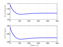
Figure 2: Feed rate $F_{in}(t)$ and Screw speed $N(t)$

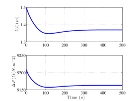
Figure 3: Interface $l(t)$ and pressure difference $\Delta P(t)$

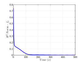
Figure 4: Filling ratio $\|f_{p}(t,\cdot)-f_{p_{e}}\|_{H^{2}(0,1)}$

V Conclusion

In this paper, we study the stabilization of a physical model for the extrusion process, which is described by conservation laws coupled through a dynamical interface. The exponential stabilization is obtained for the closed-loop system with natural feedback controls through indirect measurements. The proof relies on Lyapunov approach. Numerical simulations are made as supplementary to the theoretical results. As a future work, it is interesting to study the controllability of boundary profile, i.e., to reach the desired moisture and temperature at the die under suitable controls. This problem is rather challenging for mathematical theory but also very useful in applications. The proposed result is a first step towards controlling complex screw extrusion systems that include unknown parameters and time-varying disturbances acting on the pressure dynamics and the viscosity in the FFZ.

Physical definition of the parameters
$L=2$ $m$ Extruder Length $B=2.4\times 10^{-6}$ $m^{4}$ Geometric parameter $K_{d}=2.4\times 10^{-3}$ $m^{3}$ Geometric parameter $\zeta=0.003$ $m$ Screw Pitch $\eta=125$ $Pa$ $s^{-1}$ Melt viscosity $\rho_{o}=350$ $kg$ $m^{-3}$ Melt density $S_{eff}=0.014$ $m^{2}$ Effective area $V_{eff}=\zeta S_{eff}$ Effective volume

Proof of Proposition 2. It suffices to consider the existence of $k_{1}$ satisfying (11). Case 1) $a_{1}<0$. (11) is true for $k_{1}\rightarrow 0$. Case 2) $a_{1}\geqslant 0$ and $a_{2}b_{1}\neq 0$. If $b_{2}=0$, (11) is true either for $k_{1}\rightarrow+\infty$ or for $k_{1}\rightarrow-\infty$; If $b_{2}\neq 0$, (11) is true either for $k_{1}\rightarrow\displaystyle\frac{1}{b_{2}}+$ or for $k_{1}\rightarrow\displaystyle\frac{1}{b_{2}}-$. Upon the existence of $k_{1}$, (12) is true either for $k_{2}$ is arbitrary if $a_{3}b_{1}=0$ or for $k_{2}\rightarrow f_{p_{e}}\rho_{o}V_{eff}k_{1}$ if $a_{3}b_{1}\neq 0$. ∎

References

• [1] J-M. Coron. Control and nonlinearity, volume 136 of Mathematical Surveys and Monographs. American Mathematical Society, Providence, RI, 2007.
• [2] J-M. Coron, G. Bastin, and B. d’Andréa Novel. Dissipative boundary conditions for one-dimensional nonlinear hyperbolic systems. SIAM J. Control Optim., 47(3):1460–1498, 2008.
• [3] J-M. Coron, B. d’Andréa Novel, and G. Bastin. A strict lyapunov function for boundary control of hyperbolic systems of conservation laws. IEEE Trans. Automat. Control, 52(1):2–11, 2007.
• [4] J.-M. Coron, B. d’Andréa Novel, and G. Bastin. A lyapunov approach to control irrigation canals modeled by saint venant equations. Proc. Eur. Control Conf.,Karlruhe, Germany, Sep. 1999.
• [5] J-M. Coron and Z. Q. Wang. Output feedback stabilization for a scalar conservation law with a nonlocal velocity. SIAM J. Math. Analysis, 45(5):2646–2665, 2013.
• [6] A. Diagne, G. Bastin, and J.-M. Coron. Lyapunov exponential stability of 1-D linear hyperbolic systems of balance laws. Automatica J. IFAC, 48(1):109–114, 2012.
• [7] M. Diagne, V. Dos Santos Martins, F. Couenne, and B. Maschke. Well posedness of the model of an extruder in infinite dimension. In Decision and Control and European Control Conference (CDC-ECC), 2011 50th IEEE Conference on, pages 1311–1316, 2011.
• [8] M. Diagne, P. Shang, and Z. Q. Wang. Cauchy problem for coupled hyperbolic systems through a moving interface. arXiv:1404.3375, 2014.
• [9] Mamadou Diagne, Francoise Couenne, and Bernhard Maschke. Mass transport equation with moving interface and its control as an input delay system. In IFAC, 11th Workshop on Time-Delay Systems, WTC, Grenoble, France, volume 11, 2013.
• [10] J. Elsey, J. Riepenhausen, B. Mckay, G.W. Barton, and M. Willis. Modeling and control of a food extrusion process. Computers Chemical Engineering, 21:361–366, 1997.
• [11] J. M. Greenberg and Tatsien Li. The effect of boundary damping for the quasilinear wave equation. J. Differential Equations, 52(1):66–75, 1984.
• [12] M. Gugat, G. Leugering, S. Tamasoiu, and K. Wang. $H^{2}$-stabilization of the isothermal Euler equations: a Lyapunov function approach. Chin. Ann. Math. Ser. B, 33(4):479–500, 2012.
• [13] M.K. Kulshreshtha, Claudio A Zaror, and David J Jukes. Simulating the performance of a control system for food extruders using model-based set-point adjustment. Food Control, 6:135–141, 1995.
• [14] M.K. Kulshrestha and C.A. Zaror. An unsteady state model for twin screw extruders. Tran IChemE, PartC, 70:21–28, 1992.
• [15] C-H. Li. Modelling extrusion cooking. Mathematical and Computer Modelling, 33:553–563, 2001.
• [16] T.-T. Li. Global classical solutions for quasilinear hyperbolic systems. Research in Applied Mathematics. Masson and Viley, Berlin, 1994.
• [17] Q Lu, SJ Mulvaney, F Hsieh, and HE Huff. Model and strategies for computer control of a twin-screw extruder. Food Control, 4(1):25–33, 1993.
• [18] M. McAfee and S. Thompson. A novel approach to dynamic modeling of polymer extrusion for improved process control. Systems and Control Engineering, 221:617–627, 2007.
• [19] R.G. Moreira, A.K. Srivastava, and J.B. Gerrish. Feedforward control model for a twin-screw food extruder. Food Control, 6:361–386, July 1990.
• [20] S.A. Nield, H.M. Budman, and C. Tzoganakis. Control of a LPDE reactive extrusion process. Control Engineering Practice, 8:911–920, 2000.
• [21] J. R. Pacrez-Correa and C. A. Zaror. Recent advances in process control and their potential applications to food processing. Food Control, 4(4):202–209, 1993.
• [22] A. Tchousso, T. Besson, and C-Z. Xu. Exponential stability of distributed parameter systems governed by symmetric hyperbolic partial differential equations using Lyapunov’s second method. ESAIM Control Optim. Calc. Var., 15(2):403–425, 2009.
• [23] C-Z. Xu and G. Sallet. Exponential stability and transfer functions of processes governed by symmetric hyperbolic systems. ESAIM Control Optim. Calc. Var., 7:421–442 (electronic), 2002.