A law of the iterated logarithm for Grenander’s estimator

Abstract

In this note we prove the following law of the iterated logarithm for the Grenander estimator of a monotone decreasing density: If $f(t_{0})>0$, $f^{\prime}(t_{0})<0$, and $f^{\prime}$ is continuous in a neighborhood of $t_{0}$, then

$$\phantom{bla}\limsup_{n\rightarrow\infty}\left(\frac{n}{2\log\log n}\right)^{1/3}(\widehat{f}_{n}(t_{0})-f(t_{0}))=\left|f(t_{0})f^{\prime}(t_{0})/2\right|^{1/3}2M$$

almost surely where

$$M\equiv\sup_{g\in{\cal G}}T_{g}=(3/4)^{1/3}\ \ \ \mbox{and}\ \ \ T_{g}\equiv\mathop{\rm argmax}_{u}\{g(u)-u^{2}\};$$

here ${\cal G}$ is the two-sided Strassen limit set on ${\mathbb{R}}$. The proof relies on laws of the iterated logarithm for local empirical processes, Groeneboom’s switching relation, and properties of Strassen’s limit set analogous to distributional properties of Brownian motion.

label=e1]lutz.duembgen@stat.unibe.ch label=e2]jaw@stat.washington.edu and label=e3]m.lee.wolff@gmail.com

t1Supported in part by Swiss National Science Foundation t2Supported in part by NSF Grant DMS-1104832 and NI-AID grant 2R01 AI291968-04

1 Introduction: the MLE of a monotone density

Nonparametric estimation of a monotone density was first considered by Grenander [1956]. Suppose that $X_{1},\ldots,X_{n}$ are i.i.d. with distribution function $F$ on $[0,\infty)$ having a decreasing density $f$. Grenander showed that the maximum likelihood estimator $\hat{f}_{n}$ of $f$ is the (left-) derivative of the least concave majorant of the empirical distribution function ${\mathbb{F}}_{n}$

$$\widehat{f}_{n} = \{\mbox{left derivative of the least concave majorant of }{\mathbb{F}}_{n}\}.$$

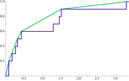
Figure 1: Empirical distribution and Least concave majorant, $n=10$

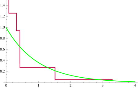
Figure 2: Grenander Estimator and Exp(1) density, $n=10$

The asymptotic distribution of $\hat{f}_{n}(t_{0})$ at a fixed point $t_{0}$ with $f^{\prime}(t_{0})<0$ was obtained by Prakasa Rao [1969], and given a somewhat different proof by Groeneboom [1985]. If $f^{\prime}(t_{0})<0$ and $f^{\prime}$ is continuous in a neighborhood of $t_{0}$, then

$$n^{1/3}(\widehat{f}_{n}(t_{0})-f(t_{0}))\rightarrow_{d}\Big{|}\frac{1}{2}f(t_{0})f^{\prime}(t_{0})\Big{|}^{1/3}2{\mathbb{Z}},$$ (1.1)

where

$$2{\mathbb{Z}} \ = \mbox{slope at 0 of the least concave majorant of }\ \ W(t)-t^{2}\,$$

$$\stackrel{{\scriptstyle d}}{{=}} \mbox{slope at 0 of the greatest convex }\ \mbox{minorant of }\ \ W(t)+t^{2}$$

$$\stackrel{{\scriptstyle d}}{{=}} 2\,\mathop{\rm argmin}_{t\in{\mathbb{R}}}\{W(t)+t^{2}\};$$

here $\{W(t):\ t\in{\mathbb{R}}\}$ is a two-sided Brownian motion process starting at $0$. In fact, the convergence in (1.1) can be extended to weak convergence of the (local) Grenander process as follows. Let $\{{\mathbb{S}}_{a,b}(t):\ t\in{\mathbb{R}}\}$ denote the slope process corresponding to the least concave majorant of $X_{a,b}(t)=aW(t)-bt^{2}$, with $a=\sqrt{f(t_{0})}$ and $b=|f^{\prime}(t_{0})|/2$. Then for fixed $t_{0}$ with $f^{\prime}(t_{0})<0$ and $f^{\prime}$ continuous in a neighborhood of $t_{0}$,

$$n^{1/3}(\hat{f}_{n}(t_{0}+n^{-1/3}t)-f(t_{0}))\Rightarrow{\mathbb{S}}_{a,b}(t)$$

in the Skorokhod topology on $D[-K,K]$ for every finite $K>0$; see e.g. Groeneboom [1989], Kim and Pollard [1990], and Huang and Zhang [1994]. Groeneboom [1989] gives a complete analytic characterization of the limiting distribution ${\mathbb{Z}}$ and further, the distributional structure of the process ${\mathbb{S}}$. The distribution of ${\mathbb{Z}}={\mathbb{S}}(0)/2$ has been studied numerically by Groeneboom and Wellner [2001] which relies heavily on Groeneboom [1985] and Groeneboom [1989]. Balabdaoui and Wellner [2014] show that the distribution of ${\mathbb{Z}}$ is log-concave. Note that there is an “invariance principle” involved here: the centered slope of the least concave majorant of ${\mathbb{F}}_{n}$ converges weakly to a constant times the slope of the least concave majorant of $X(t)=W(t)-t^{2}$. We can regard the slope in this Gaussian limit problem, $2{\mathbb{Z}}$, as an “estimator” of the slope of the line $2t$ in the Gaussian problem of “estimating” the “canonical” linear function $2t$ in “Gaussian white noise” $dW(t)$ since

$$dX(t)=2tdt+dW(t)\,.$$

2 A law of the iterated logarithm for the Grenander estimator

Our main goal is to prove the following Law of the Iterated Logarithm (LIL) for the Grenander estimator corresponding to the limiting distribution result in (1.1).

Theorem 1.

Suppose that $f(t_{0})>0$, $f_{0}^{\prime}(t_{0})<0$ with $f^{\prime}$ continuous in a neighborhood of $t_{0}$. Then

$$\limsup_{n\rightarrow\infty}\frac{n^{1/3}(\widehat{f}_{n}(t_{0})-f(t_{0}))}{(2\log\log n)^{1/3}}\ =\ \Big{|}\frac{1}{2}f(t_{0})f^{\prime}(t_{0})\Big{|}^{1/3}2M$$

almost surely where

$$M\equiv\sup_{g\in{\cal G}}\mathop{\rm argmax}_{t\in{\mathbb{R}}}\{g(t)-t^{2}\}=\left(\frac{3}{4}\right)^{1/3};$$

here ${\cal G}$ is the two-sided Strassen limit set on ${\mathbb{R}}$ given by

$${\cal G}\ =\ \left\{g:{\mathbb{R}}\rightarrow{\mathbb{R}}\,\big{|}\,g(t)=\int_{0}^{t}\dot{g}(s)ds,\ t\in{\mathbb{R}},\ \ \int_{-\infty}^{\infty}\dot{g}^{2}(s)ds\leq 1\right\}\,.$$ (2.1)

Our proof of Theorem 1 will rely on functional laws of the iterated logarithm for the local empirical process established by Mason [1988]; see also Deheuvels and Mason [1994], Einmahl and Mason [1998], Einmahl and Mason [1997], and Mason [2004]. Along the way we will also prove several lemmas concerning the limit set ${\cal G}$.

Proof.

We begin the proof of Theorem 1 with a switching argument. Let $b_{n}\equiv(n^{-1}2\log\log n)^{1/3}$. Then we want to find a number $x_{0}$ such that

$$P(b_{n}^{-1}(\widehat{f}_{n}(t_{0})-f(t_{0}))>x\ \ \mbox{i.o.})=\left\{\begin{array}[]{l l}0,&\ \ \mbox{if}\ x>x_{0},\\ 1,&\ \ \mbox{if}\ x<x_{0}.\end{array}\right.$$

Now we let

$$\widehat{s}_{n}(a)\equiv\mathop{\rm argmax}_{s}\{{\mathbb{F}}_{n}(s)-as\},\ \ a\geq 0,$$ (2.3)

and note that $\{\widehat{f}_{n}(t_{0})>a\}=\{\widehat{s}_{n}(a)>t_{0}\}$ by Groeneboom’s switching relation (see e.g. Groeneboom [1985], van der Vaart and Wellner [1996] page 296, and Balabdaoui et al. [2011], Theorem 2.1, page 881). Thus the event in the last display can be rewritten as

$$\left\{\widehat{f}_{n}(t_{0})>f(t_{0})+b_{n}x\ \ \mbox{i.o.}\right\} = \left\{\widehat{s}_{n}(f(t_{0})+b_{n}x)>t_{0}\ \ \mbox{i.o.}\right\}.$$ (2.4)

But, by letting $s=t_{0}+b_{n}h$ in (2.3) we see that

$$\widehat{s}_{n}(f(t_{0})+b_{n}x)-t_{0} = b_{n}\mathop{\rm argmax}_{h}\{{\mathbb{F}}_{n}(t_{0}+b_{n}h)-(f(t_{0})+b_{n}x)(t_{0}+b_{n}h)\},$$

and hence the right side of (2.4) can be rewritten as $\{\widehat{h}_{n}>0\ \mbox{i.o.}\}$ where

$$\widehat{h}_{n} = \mathop{\rm argmax}_{h}\{{\mathbb{F}}_{n}(t_{0}+b_{n}h)-(f(t_{0})+b_{n}x)(t_{0}+b_{n}h)\}$$ (2.5)

$$= \mathop{\rm argmax}_{h}\left\{b_{n}^{-2}\{{\mathbb{F}}_{n}(t_{0}+b_{n}h)-{\mathbb{F}}_{n}(t_{0})-(F(t_{0}+b_{n}h)-F(t_{0}))\}\right.$$

$$\qquad\left.+\ b_{n}^{-2}\{F(t_{0}+b_{n}h)-F(t_{0})-f(t_{0})b_{n}h\}-xh\right\}.$$

The second term on the right side in the last display converges to $f^{\prime}(t_{0})h^{2}/2$ as $n\rightarrow\infty$. The handle the first term we appeal to (a slight extension of) Theorem 2 of Mason [1988]; see also Deheuvels and Mason [1994] Theorem A and Theorem 1.1, pages 1620-1621: by considering $h\in{\mathbb{R}}$ and introducing the two-sided version ${\cal G}$ of the Strassen limit set given in (2.1) much as in Wichura [1974], we see that the sequence of functions

$$\left\{b_{n}^{-2}\{{\mathbb{F}}_{n}(t_{0}+b_{n}h)-{\mathbb{F}}_{n}(t_{0})-(F(t_{0}+b_{n}h)-F(t_{0}))\}:\ h\in{\mathbb{R}}\right\}$$

is almost surely relatively compact with limit set

$$\{g(f(t_{0})\cdot):\ g\in{\cal G}\}$$

where ${\cal G}$ is given by (2.1).

This is most easily seen as follows: let ${\mathbb{G}}_{n}$ be the empirical d.f. of $\xi_{1},\ldots,\xi_{n}$ i.i.d. Uniform$(0,1)$. As in Deheuvels and Mason [1994], with $n^{-1}k_{n}\equiv b_{n}$ so that $k_{n}=nb_{n}=n^{2/3}(2\log\log n)^{1/3}\nearrow\infty$ and $n^{-1}k_{n}=b_{n}\searrow 0$, the processes

$$\frac{\xi_{n}(s)}{\sqrt{2\log\log n}}$$

$$= \frac{n^{1/2}}{\sqrt{k_{n}/n}}\frac{\left\{{\mathbb{G}}_{n}(F(t_{0}+n^{-1}k_{n}s))-{\mathbb{G}}_{n}(F(t_{0}))-(F(t_{0}+n^{-1}k_{n}s)-F(t_{0}))\right\}}{\sqrt{2\log\log n}}$$

with $s\geq 0$ are almost surely relatively compact with limit set ${\cal K}_{\infty}(c)\equiv\{t\mapsto g(ct):\ g\in{\cal K}_{\infty}\}$ with $c=f(t_{0})$. Here we also note that

$$\frac{n^{1/2}}{\sqrt{k_{n}/n}\sqrt{2\log\log n}}=\frac{n^{2/3}}{(2\log\log n)^{2/3}}=b_{n}^{-2}.$$

Thus the processes involved in the argmax in (2.5) are almost surely relatively compact with limit set

$$\{g(f(t_{0})h)+2^{-1}f^{\prime}(t_{0})h^{2}-xh:\ \ g\in{\cal G}\},$$

and by Lemma 1 below this set is equal to

$$\left\{ag(h)-bh^{2}-xh:\ \ g\in{\cal G}\right\}$$

where $a\equiv\sqrt{f(t_{0})}$, and $b=|f^{\prime}(t_{0})|/2$. Thus by Lemma 2 below, the set of limits for the argmax in (2.5) equals

$$\left\{(a/b)^{2/3}\mathop{\rm argmax}_{h}\{g(h)-h^{2}\}-x/(2b):\ \ g\in{\cal G}\right\}$$

where

$$\left(\frac{a}{b}\right)^{2/3}=\left(\frac{\sqrt{f(t_{0})}}{2^{-1}|f^{\prime}(t_{0})|}\right)^{2/3}=\left(\frac{4f(t_{0})}{|f^{\prime}(t_{0})|^{2}}\right)^{1/3}.$$

Hence, with $T_{g}=\mathop{\rm argmax}_{h}\{g(h)-h^{2}\}$,

$$\left\{\widehat{h}_{n}>0\ \ \mbox{i.o.}\right\} \stackrel{{\scriptstyle a.s.}}{{=}} \left\{\left(\frac{a}{b}\right)^{2/3}\sup_{g\in{\cal G}}T_{g}>\frac{x}{2b}\right\}$$

$$= \left\{2b\left(\frac{a}{b}\right)^{2/3}\sup_{g\in{\cal G}}T_{g}>x\right\}$$

$$= \emptyset$$

if

$$x>x_{0}\equiv 2b\left(\frac{a}{b}\right)^{2/3}\sup_{g\in{\cal G}}T_{g}=\Big{|}\frac{1}{2}f(t_{0})f^{\prime}(t_{0})\Big{|}^{1/3}2\sup_{g\in{\cal G}}T_{g}.$$

It remains only to show that $\sup_{g\in{\cal G}}T_{g}=(3/4)^{1/3}$. This follows from Lemma 3 in Section 4 below. ∎

Lemma 1.

Let $c>0$ and $d\in{\mathbb{R}}$. Then

$$\left\{t\mapsto g(ct+d)-g(d):\ g\in{\cal G}\right\}=\sqrt{c}{\cal G}.$$

Proof.

If $g\in{\cal G}$, then

$$g(ct+d)-g(d) = \int_{d}^{ct+d}\dot{g}(s)ds=\int_{0}^{ct}\dot{g}(v+d)dv=\int_{0}^{t}\dot{g}(cu+d)cdu$$

$$= \sqrt{c}\int_{0}^{t}\sqrt{c}\dot{g}(cu+d)du$$

$$= \sqrt{c}\tilde{g}(t)$$

where $\tilde{g}\in{\cal G}$ since

$$\int_{-\infty}^{\infty}(\sqrt{c}\dot{g}(cu+d))^{2}du=\int_{-\infty}^{\infty}\dot{g}^{2}(w)dw\leq 1.$$

This shows that the set of functions $t\mapsto g(ct+d)-g(d)$, $g\in{\cal G}$, is contained in $\sqrt{c}{\cal G}$. On the other hand, any function $\tilde{g}\in{\cal G}$ with derivative $\dot{\tilde{g}}$ may be written as $\tilde{g}(t)=\int\sqrt{c}\dot{g}(cu+d)du$ with $\dot{g}$ given by $\dot{g}(s)\equiv\sqrt{c^{-1}}\dot{\tilde{g}}(c^{-1}s-c^{-1}d)$ and satisfying $\int_{-\infty}^{\infty}\dot{g}(s)^{2}ds=\int_{-\infty}^{\infty}\dot{\tilde{g}}(s)^{2}ds\leq 1$. ∎

Lemma 2.

Let $\alpha,\beta$ be positive constants and $\gamma\in{\mathbb{R}}$. Then

$$\left\{\mathop{\rm argmax}_{h}\{\alpha g(h)-\beta h^{2}-\gamma h\}:\ \ g\in{\cal G}\right\}$$ (2.6)

$$= \left\{(\alpha/\beta)^{2/3}\mathop{\rm argmax}_{h}\{g(h)-h^{2}\}-\gamma/(2\beta):\ \ g\in{\cal G}\right\}.$$

Proof.

Note first that

$$M_{g} \equiv \mathop{\rm argmax}_{h}\left\{\alpha g(h)-\beta h^{2}-\gamma h\right\}$$

$$= \mathop{\rm argmax}_{h}\left\{\alpha g(h)-\beta(h+\gamma/(2\beta))^{2}\right\}$$

$$= \mathop{\rm argmax}_{h}\left\{g(h)-(\beta/\alpha)(h+\gamma/(2\beta))^{2}\right\}$$

$$= \mathop{\rm argmax}_{v}\left\{g(v+d)-(\beta/\alpha)v^{2}\right\}+d$$

with $d:=-\gamma/(2\beta)$. Moreover, for any $c>0$ and

$$\tilde{g}(u)\equiv c^{-1/2}\left(g(cu+d)-g(d)\right)$$

we may write

$$M_{g} = c\mathop{\rm argmax}_{u}\left\{g(cu+d)-g(d)-(\beta/\alpha)c^{2}u^{2}\right\}+d$$

$$= c\mathop{\rm argmax}_{u}\left\{c^{1/2}\tilde{g}(u)-(\beta/\alpha)c^{2}u^{2}\right\}+d$$

$$= c\mathop{\rm argmax}_{u}\left\{\tilde{g}(u)-(\beta/\alpha)c^{3/2}u^{2}\right\}+d.$$

In case of $c=(\alpha/\beta)^{2/3}$ we obtain

$$M_{g}=(\alpha/\beta)^{2/3}\mathop{\rm argmax}_{u}\left\{\tilde{g}(u)-u^{2}\right\}-\gamma/(2\beta).$$

Now the claim follows from Lemma 1, because the set $\left\{\tilde{g}:g\in{\cal G}\right\}$ equals ${\cal G}$. ∎

3 Some comparisons and connections

As noted in the introduction,

$$2{\mathbb{Z}}\stackrel{{\scriptstyle d}}{{=}}\mbox{slope at zero of the least concave majorant of}\ \ W(t)-t^{2}.$$

This suggests that with $T_{g}=\mbox{argmax}_{t}\{g(t)-t^{2}\}$ we have

$$\left\{2\sup T_{g}:\ g\in{\cal G}\right\}$$

$$= \sup\{\mbox{slope at}\ 0\ \mbox{of the least concave majorant of }\ g(t)-t^{2}:\ g\in{\cal G}\}.$$

4 Proof for the variational problem

It is natural to conjecture that $\sup_{g\in{\cal G}}T_{g}=(3/4)^{1/3}\approx 0.90856\ldots$. This is motivated by the asymptotic behavior of Chernoff’s density; see Groeneboom [1989], Corollary 3.4, page 94: since the density

$$f_{{\mathbb{Z}}}(z)\sim\frac{1}{2Ai^{\prime}(a_{1})}4^{4/3}z\exp\left(-\frac{2}{3}z^{3}+3^{1/3}a_{1}z\right)$$

as $z\rightarrow\infty$, the tail probability $P({\mathbb{Z}}>z)$ satisfies

$$P({\mathbb{Z}}>z)\sim\frac{1}{2Ai^{\prime}(a_{1})}4^{4/3}\frac{1}{z}\exp\left(-\frac{2}{3}z^{3}\right)$$

as $z\rightarrow\infty$ where $a_{1}\dot{=}-2.3381$ is the largest zero of the Airy function $Ai$ and $Ai^{\prime}(a_{1})\dot{=}0.7022$. Thus from (1.1) we expect that

$$\limsup_{n\rightarrow\infty}\frac{n^{1/3}(\widehat{f}_{n}(t_{0})-f(t_{0}))}{((3/2)\log\log n)^{1/3}}\ =\ \Big{|}\frac{1}{2}f(t_{0})f^{\prime}(t_{0})\Big{|}^{1/3}2,$$

or, equivalently,

$$\limsup_{n\rightarrow\infty}\frac{n^{1/3}(\widehat{f}_{n}(t_{0})-f(t_{0}))}{(2\log\log n)^{1/3}} \ =\ \Big{|}\frac{1}{2}f(t_{0})f^{\prime}(t_{0})\Big{|}^{1/3}2\cdot\frac{1}{2^{1/3}}\cdot\left(\frac{3}{2}\right)^{1/3}$$

$$\ =\ \Big{|}\frac{1}{2}f(t_{0})f^{\prime}(t_{0})\Big{|}^{1/3}2\cdot\left(\frac{3}{4}\right)^{1/3}.$$

On the other hand the proof of Theorem 1 above leads to

$$\limsup_{n\rightarrow\infty}\frac{n^{1/3}(\widehat{f}_{n}(t_{0})-f(t_{0}))}{(2\log\log n)^{1/3}} \ =\ \Big{|}\frac{1}{2}f(t_{0})f^{\prime}(t_{0})\Big{|}^{1/3}2\cdot M\ \ \ \mbox{a.s.}$$

where

$$M\equiv\sup_{g\in{\cal G}}\mbox{argmax}_{t\in{\mathbb{R}}}\{g(t)-t^{2}\}\equiv\sup_{g\in{\cal G}}T_{g}.$$

Thus we conjecture that $M=(3/4)^{1/3}$.

Lemma 3.

Let $t_{0}>0$ be an arbitrary positive number and let $\dot{g}\in L_{1}([0,t_{0}])$ be an arbitrary function satisfying

$$\int_{0}^{t_{0}}\dot{g}(s)ds-t_{0}^{2}\geq\int_{0}^{t}\dot{g}(s)ds-t^{2}\ \ \ \mbox{for}\ \ 0\leq t\leq t_{0}.$$

Then

$$\int_{0}^{t_{0}}\dot{g}(u)^{2}du\geq\int_{0}^{t_{0}}(2u)^{2}du=\frac{4t_{0}^{3}}{3}.$$

Proof.

Let $\dot{g}_{0}(u)\equiv 2u$. The claimed inequality is trivial if the integral on the left side is infinite, so we may view $\dot{g}$ and $\dot{g_{0}}$ as elements of the Hilbert space $L_{2}([0,t_{0}])$. Then the assumption on $\dot{g}$ may be rewritten as

$$\langle\dot{g}-\dot{g}_{0},1\rangle\geq\langle\dot{g}-\dot{g}_{0},1_{[0,t]}\rangle\ \ \mbox{for}\ \ 0\leq t\leq t_{0}.$$

In other words,

$$\langle\dot{g}-\dot{g}_{0},1_{(t,t_{0}]}\rangle\geq 0\ \ \ \mbox{for}\ \ 0\leq t\leq t_{0},$$

and this is equivalent to

$$\langle\dot{g}-\dot{g}_{0},f\rangle\geq 0$$

for all functions $f$ in the closed convex cone ${\mathbb{K}}$ generated by the indicator functions $1_{(t,t_{0}]}$. This is the set of non-negative and non-decreasing functions on $[0,t_{0}]$. In particular, $\dot{g}_{0}\in{\mathbb{K}}$, so

$$\langle\dot{g}-\dot{g}_{0},\dot{g}_{0}\rangle\geq 0.$$

Together with the Cauchy-Schwarz inequality we obtain

$$0\leq\langle\dot{g}-\dot{g}_{0},\dot{g}_{0}\rangle=\langle\dot{g},\dot{g}_{0}\rangle-\|\dot{g}_{0}\|^{2}\leq\|\dot{g}\|\|\dot{g}_{0}\|-\|\dot{g}_{0}\|^{2},$$

so $\|\dot{g}\|\geq\|\dot{g}_{0}\|$. This inequality is strict unless $\dot{g}=\lambda\dot{g}_{0}$ for some $\lambda\in{\mathbb{R}}$. In this special case the last display reads $0\leq(\lambda-1)\|\dot{g}_{0}\|^{2}$, so $\lambda\geq 1$ and $\|\dot{g}\|=\lambda\|\dot{g}_{0}\|$ with equality if, and only if, $\lambda=1$ and $\dot{g}=\dot{g}_{0}$. ∎

Example 1.

If we take $f(x)=e^{-x}1_{[0,\infty)}(x)$ and $t_{0}=\log 2$, then

$$\Big{|}\frac{1}{2}f(t_{0})f^{\prime}(t_{0})\Big{|}^{1/3}\cdot 2=(2^{-3})^{1/3}\cdot 2=1,$$

so the limit superior is just $\sup_{g\in{\cal G}}T_{g}=(3/4)^{1/3}$.

Example 2.

If we take $f(x)=(1+x)^{-2}1_{[0,\infty)}(x)$, then $-f^{\prime}(x)=2(1+x)^{-3}$ and hence with $t_{0}=1$ we have $f(1)=1/4=-f^{\prime}(1)$. Then

$$\Big{|}\frac{1}{2}f(t_{0})f^{\prime}(t_{0})\Big{|}^{1/3}\cdot 2=(2^{-5/3})\cdot 2=2^{-2/3},$$

so the limit superior is $2^{-2/3}\sup_{g\in{\cal G}}T_{g}=(3/16)^{1/3}$.

Example 3.

If we take $f(x)=(\sqrt{2}-x)1_{[0,\sqrt{2}]}(x)$ and $t_{0}=\sqrt{2}-1$, then $f(t_{0})=1$, $-f^{\prime}(t_{0})=1$, and

$$\Big{|}\frac{1}{2}f(t_{0})f^{\prime}(t_{0})\Big{|}^{1/3}\cdot 2=(2^{-1/3})\cdot 2=2^{+2/3},$$

so the limit superior is $2^{+2/3}\sup_{g\in{\cal G}}T_{g}=2^{2/3}(3/4)^{1/3}=3^{1/3}$.

5 Some corollaries

Theorem 1 has a number of corollaries and consequences, since the argument in the proof applies to a number of problems involving nonparametric estimation of a monotone function. Our first corollary, however, involves estimation of the mixing distribution $G$ in the mixture representation of a monotone density: that is,

$$f(x)=\int_{0}^{\infty}\frac{1}{y}1_{[0,y)}(x)dG(y)=\int_{\{y>x\}}\frac{1}{y}dG(y),\qquad x\in(0,\infty)$$ (5.1)

for some distribution function $G$ on $(0,\infty)$. This fact apparently goes back at least to Schoenberg [1941]; see the introduction of Williamson [1956], and Feller [1971], page 158. The relationship (5.1) implies that the corresponding distribution function $F$ is given by

$$F(x) = \int_{0}^{\infty}\frac{x}{y}1_{[0,y)}(x)dG(y)+\int_{0}^{\infty}1_{[y,\infty)}(x)dG(y)$$

$$= xf(x)+G(x)\,,$$

and this can be “inverted” to yield

$$G(x)=F(x)-xf(x)\,.$$ (5.2)

From Figure 3 we see that the function on the right side of (5.2) is non-negative and non-decreasing: the shaded area gives exactly the difference $F(x)-xf(x)$.

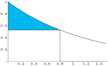
Figure 3: Graphical view of the inversion formula, monontone density

The identity (5.2) implies that the nonparametric maximum likelihood estimator of $G$ is $\widehat{G}_{n}$ given by

$$\widehat{G}_{n}(t)=\widehat{F}_{n}(t)-t\widehat{f}_{n}(t),\ \ \mbox{for}\ \ t\geq 0$$

where $\widehat{F}_{n}(t)=\int_{0}^{t}\widehat{f}_{n}(x)dx$ is the least concave majorant of ${\mathbb{F}}_{n}$ and the MLE of $F$ assuming that $f$ is monotone (and hence $F$ is concave). Thus for $t_{0}>0$ we can write

$$n^{1/3}(\widehat{G}_{n}(t_{0})-G(t_{0}))=n^{1/3}(\widehat{F}_{n}(t_{0})-F(t_{0}))-t_{0}n^{1/3}(\widehat{f}_{n}(t_{0})-f(t_{0}))$$

From Marshall’s lemma Marshall [1970] and $n^{1/2}\|{\mathbb{F}}_{n}-F\|_{\infty}=O_{p}(1)$ it follows that $n^{1/3}\|\widehat{F}_{n}-F\|_{\infty}=o_{p}(1)$. Thus if $t_{0}>0$ is a point at which the hypotheses of Theorem 1 hold, then the convergence in (1.1) implies that

$$n^{1/3}(\widehat{G}_{n}(t_{0})-G(t_{0}))\rightarrow_{d}t_{0}\Big{|}\frac{1}{2}f(t_{0})f^{\prime}(t_{0})\Big{|}^{1/3}2{\mathbb{Z}},$$ (5.3)

Similarly, from Marshall’s lemma Marshall [1970] and Chung’s law of the iterated logarithm for $\|{\mathbb{F}}_{n}-F\|_{\infty}$ (see e.g. Shorack and Wellner [1986], page 505), we know that with $b_{n}\equiv(2\log\log n)^{1/2}$

$$\limsup_{n\rightarrow\infty}n^{1/2}\|\widehat{F}_{n}-F\|_{\infty}/b_{n}\leq\limsup_{n\rightarrow\infty}n^{1/2}\|{\mathbb{F}}_{n}-F\|_{\infty}/b_{n}=1/2\ \ \mbox{a.s.}.$$

It follows that if $t_{0}>0$ is a point at which the hypotheses of Theorem 1 hold, then Theorem 1 yields a LIL result for $\widehat{G}_{n}(t_{0})$ as follows:

Collorary 1.

Suppose that $f(t_{0})>0$ and $f^{\prime}(t_{0})<0$ with $f^{\prime}$ continuous in a neighborhood of $t_{0}$. Then

$$\limsup_{n\rightarrow\infty}\frac{n^{1/3}(\widehat{G}_{n}(t_{0})-G(t_{0}))}{(2\log\log n)^{1/3}}=t_{0}\Big{|}\frac{1}{2}f(t_{0})f^{\prime}(t_{0})\Big{|}^{1/3}2(3/4)^{1/3}\$$

almost surely.

6 A further problem

For the problem of estimating a convex decreasing density, Groeneboom, Jongbloed and Wellner [2001] described the limiting distribution of the estimator (at a point under a natural curvature condition) in terms of an “invelope” of two-sided integrated Brownian motion plus $t^{4}$ which was characterized in Groeneboom, Jongbloed and Wellner [2001]. The same distribution has appeared in other nonparametric convex function estimation problems, for example for log-concave density estimation: see Balabdaoui, Rufibach and Wellner [2009]. In spite of this description of the limiting distribution for the convex density case in terms of integrated Brownian motion, almost nothing is known concerning a direct analytical description of the limit distribution comparable to the results of Groeneboom [1985, 1989] for Chernoff’s distribution. (On the other hand, a preliminary numerical investigation of the distribution is given by Azadbakhsh, Jankowski and Gao [2014].)

This leads to the following question: can some information concerning the constants involved in the limiting distribution in the convex function case be obtained by establishing LIL results analogous to those established here in the monotone case?

References

• Azadbakhsh, Jankowski and Gao [2014] {barticle}[author] \bauthor\bsnmAzadbakhsh, \bfnmMahdis\binitsM., \bauthor\bsnmJankowski, \bfnmHanna\binitsH. and \bauthor\bsnmGao, \bfnmXin\binitsX. (\byear2014). \btitleComputing confidence intervals for log-concave densities. \bjournalComput. Statist. Data Anal. \bvolume75 \bpages248–264. \bmrnumber3178372 \endbibitem
• Balabdaoui, Rufibach and Wellner [2009] {barticle}[author] \bauthor\bsnmBalabdaoui, \bfnmFadoua\binitsF., \bauthor\bsnmRufibach, \bfnmKaspar\binitsK. and \bauthor\bsnmWellner, \bfnmJon A.\binitsJ. A. (\byear2009). \btitleLimit distribution theory for maximum likelihood estimation of a log-concave density. \bjournalAnn. Statist. \bvolume37 \bpages1299–1331. \bmrnumber2509075 (2010h:62290) \endbibitem
• Balabdaoui and Wellner [2014] {barticle}[author] \bauthor\bsnmBalabdaoui, \bfnmFadoua\binitsF. and \bauthor\bsnmWellner, \bfnmJon A.\binitsJ. A. (\byear2014). \btitleChernoff’s density is log-concave. \bjournalBernoulli \bvolume20 \bpages231–244. \bmrnumber3160580 \endbibitem
• Balabdaoui et al. [2011] {barticle}[author] \bauthor\bsnmBalabdaoui, \bfnmFadoua\binitsF., \bauthor\bsnmJankowski, \bfnmHanna\binitsH., \bauthor\bsnmPavlides, \bfnmMarios\binitsM., \bauthor\bsnmSeregin, \bfnmArseni\binitsA. and \bauthor\bsnmWellner, \bfnmJon\binitsJ. (\byear2011). \btitleOn the Grenander estimator at zero. \bjournalStatist. Sinica \bvolume21 \bpages873–899. \bmrnumber2829859 \endbibitem
• Deheuvels and Mason [1994] {barticle}[author] \bauthor\bsnmDeheuvels, \bfnmPaul\binitsP. and \bauthor\bsnmMason, \bfnmDavid M.\binitsD. M. (\byear1994). \btitleFunctional laws of the iterated logarithm for local empirical processes indexed by sets. \bjournalAnn. Probab. \bvolume22 \bpages1619–1661. \bmrnumber1303659 (96e:60048) \endbibitem
• Einmahl and Mason [1997] {barticle}[author] \bauthor\bsnmEinmahl, \bfnmUwe\binitsU. and \bauthor\bsnmMason, \bfnmDavid M.\binitsD. M. (\byear1997). \btitleGaussian approximation of local empirical processes indexed by functions. \bjournalProbab. Theory Related Fields \bvolume107 \bpages283–311. \bmrnumber1440134 (98d:60060) \endbibitem
• Einmahl and Mason [1998] {bincollection}[author] \bauthor\bsnmEinmahl, \bfnmUwe\binitsU. and \bauthor\bsnmMason, \bfnmDavid M.\binitsD. M. (\byear1998). \btitleStrong approximations to the local empirical process. In \bbooktitleHigh dimensional probability (Oberwolfach, 1996). \bseriesProgr. Probab. \bvolume43 \bpages75–92. \bpublisherBirkhäuser, Basel. \bmrnumber1652321 (99h:60060) \endbibitem
• Feller [1971] {bbook}[author] \bauthor\bsnmFeller, \bfnmWilliam\binitsW. (\byear1971). \btitleAn introduction to probability theory and its applications. Vol. II. \bseriesSecond edition. \bpublisherJohn Wiley & Sons, Inc., New York-London-Sydney. \bmrnumber0270403 (42 ##5292) \endbibitem
• Grenander [1956] {barticle}[author] \bauthor\bsnmGrenander, \bfnmUlf\binitsU. (\byear1956). \btitleOn the theory of mortality measurement. I. \bjournalSkand. Aktuarietidskr. \bvolume39 \bpages70–96. \bmrnumber0086459 (19,188d) \endbibitem
• Groeneboom [1985] {binproceedings}[author] \bauthor\bsnmGroeneboom, \bfnmP.\binitsP. (\byear1985). \btitleEstimating a monotone density. In \bbooktitleProceedings of the Berkeley conference in honor of Jerzy Neyman and Jack Kiefer, Vol. II (Berkeley, Calif., 1983). \bseriesWadsworth Statist./Probab. Ser. \bpages539–555. \bpublisherWadsworth, Belmont, CA. \bmrnumber822052 (87i:62076) \endbibitem
• Groeneboom [1989] {barticle}[author] \bauthor\bsnmGroeneboom, \bfnmPiet\binitsP. (\byear1989). \btitleBrownian motion with a parabolic drift and Airy functions. \bjournalProbab. Theory Related Fields \bvolume81 \bpages79–109. \bmrnumber981568 (90c:60052) \endbibitem
• Groeneboom, Jongbloed and Wellner [2001] {barticle}[author] \bauthor\bsnmGroeneboom, \bfnmPiet\binitsP., \bauthor\bsnmJongbloed, \bfnmGeurt\binitsG. and \bauthor\bsnmWellner, \bfnmJon A.\binitsJ. A. (\byear2001). \btitleA canonical process for estimation of convex functions: the “invelope” of integrated Brownian motion $+t^{4}$. \bjournalAnn. Statist. \bvolume29 \bpages1620–1652. \bmrnumber1891741 (2003c:62075) \endbibitem
• Groeneboom and Wellner [2001] {barticle}[author] \bauthor\bsnmGroeneboom, \bfnmPiet\binitsP. and \bauthor\bsnmWellner, \bfnmJon A.\binitsJ. A. (\byear2001). \btitleComputing Chernoff’s distribution. \bjournalJ. Comput. Graph. Statist. \bvolume10 \bpages388–400. \bmrnumber1939706 \endbibitem
• Huang and Zhang [1994] {barticle}[author] \bauthor\bsnmHuang, \bfnmYouping\binitsY. and \bauthor\bsnmZhang, \bfnmCun-Hui\binitsC.-H. (\byear1994). \btitleEstimating a monotone density from censored observations. \bjournalAnn. Statist. \bvolume22 \bpages1256–1274. \bmrnumber1311975 (95m:62085) \endbibitem
• Kim and Pollard [1990] {barticle}[author] \bauthor\bsnmKim, \bfnmJeanKyung\binitsJ. and \bauthor\bsnmPollard, \bfnmDavid\binitsD. (\byear1990). \btitleCube root asymptotics. \bjournalAnn. Statist. \bvolume18 \bpages191–219. \bmrnumber1041391 (91f:62059) \endbibitem
• Marshall [1970] {bincollection}[author] \bauthor\bsnmMarshall, \bfnmAlbert W.\binitsA. W. (\byear1970). \btitleDiscussion on Barlow and van Zwet’s paper. In \bbooktitleNonparametric Techniques in Statistical Inference, (\beditor\bfnmMadan Lal\binitsM. L. \bsnmPuri, ed.). \bseriesProceedings of the First International Symposium on Nonparametric Techniques held at Indiana University, June \bvolume1969 \bpages174–176. \bpublisherCambridge University Press, \baddressLondon. \bmrnumberMR0273755 (42 ##8632) \endbibitem
• Mason [1988] {barticle}[author] \bauthor\bsnmMason, \bfnmDavid M.\binitsD. M. (\byear1988). \btitleA strong invariance theorem for the tail empirical process. \bjournalAnn. Inst. H. Poincaré Probab. Statist. \bvolume24 \bpages491–506. \bmrnumber978022 (89m:60076) \endbibitem
• Mason [2004] {barticle}[author] \bauthor\bsnmMason, \bfnmDavid M.\binitsD. M. (\byear2004). \btitleA uniform functional law of the logarithm for the local empirical process. \bjournalAnn. Probab. \bvolume32 \bpages1391–1418. \bmrnumber2060302 (2005f:60080) \endbibitem
• Prakasa Rao [1969] {barticle}[author] \bauthor\bsnmPrakasa Rao, \bfnmB. L. S.\binitsB. L. S. (\byear1969). \btitleEstimation of a unimodal density. \bjournalSankhyā Ser. A \bvolume31 \bpages23–36. \bmrnumber0267677 (42 ##2579) \endbibitem
• Schoenberg [1941] {barticle}[author] \bauthor\bsnmSchoenberg, \bfnmI. J.\binitsI. J. (\byear1941). \btitleOn integral representations of completely monotone and related functions (abstract). \bjournalBull. Amer. Math. Soc. \bvolume47 \bpages208. \endbibitem
• Shorack and Wellner [1986] {bbook}[author] \bauthor\bsnmShorack, \bfnmGalen R.\binitsG. R. and \bauthor\bsnmWellner, \bfnmJon A.\binitsJ. A. (\byear1986). \btitleEmpirical processes with applications to statistics. \bseriesWiley Series in Probability and Mathematical Statistics: Probability and Mathematical Statistics. \bpublisherJohn Wiley & Sons, Inc., New York. \bmrnumber838963 (88e:60002) \endbibitem
• van der Vaart and Wellner [1996] {bbook}[author] \bauthor\bparticlevan der \bsnmVaart, \bfnmAad W.\binitsA. W. and \bauthor\bsnmWellner, \bfnmJon A.\binitsJ. A. (\byear1996). \btitleWeak convergence and empirical processes. \bseriesSpringer Series in Statistics. \bpublisherSpringer-Verlag, New York \bnoteWith applications to statistics. \bmrnumber1385671 (97g:60035) \endbibitem
• Wichura [1974] {barticle}[author] \bauthor\bsnmWichura, \bfnmMichael J.\binitsM. J. (\byear1974). \btitleFunctional laws of the iterated logarithm for the partial sums of I.I.D. random variables in the domain of attraction of a completely asymmetric stable law. \bjournalAnn. Probability \bvolume2 \bpages1108–1138. \bmrnumber0358950 (50 ##11407) \endbibitem
• Williamson [1956] {barticle}[author] \bauthor\bsnmWilliamson, \bfnmR. E.\binitsR. E. (\byear1956). \btitleMultiply monotone functions and their Laplace transforms. \bjournalDuke Math. J. \bvolume23 \bpages189–207. \bmrnumber0077581 (17,1061d) \endbibitem