Statistical ConvNet Features for Dynamic Texture and Scene Classification

Dynamic texture and scene classification by transferring deep image features

Abstract

Dynamic texture and scene classification are two fundamental problems in understanding natural video content. Extracting robust and effective features is a crucial step towards solving these problems. However the existing approaches suffer from the sensitivity to either varying illumination, or viewpoint changing, or even camera motion, and/or the lack of spatial information. Inspired by the success of deep structures in image classification, we attempt to leverage a deep structure to extract feature for dynamic texture and scene classification. To tackle with the challenges in training a deep structure, we propose to transfer some prior knowledge from image domain to video domain. To be specific, we propose to apply a well-trained Convolutional Neural Network (ConvNet) as a mid-level feature extractor to extract features from each frame, and then form a representation of a video by concatenating the first and the second order statistics over the mid-level features. We term this two-level feature extraction scheme as a Transferred ConvNet Feature (TCoF). Moreover we explore two different implementations of the TCoF scheme, i.e., the spatial TCoF and the temporal TCoF, in which the mean-removed frames and the difference between two adjacent frames are used as the inputs of the ConvNet, respectively. We evaluate systematically the proposed spatial TCoF and the temporal TCoF schemes on three benchmark data sets, including DynTex, YUPENN, and Maryland, and demonstrate that the proposed approach yields superior performance.

1 Introduction

Dynamic texture and dynamic scene classification are two fundamental problems in understanding natural video content and have gained considerable research attention [39, 27, 14, 40, 13, 12, 31, 6, 37, 16, 11, 20, 15, 34]. Roughly, dynamic textures can be described as visual processes, which consist of a group of particles with random motions; dynamic scenes can be considered as places where events occur. In Fig. 1, we show some sample images from a dynamic scene data set YUPENN [11]. The ability to automatically categories dynamic textures or scenes is useful, since it can be used to recognize the presence of events, surfaces, actions, and phenomena in a video surveillance system.

However automatically categorizing dynamic textures or dynamic scenes is a challenging problem, since the existence of a wide range of naturally occurring variations in a short video, e.g., illumination variations, viewpoint changes, or even significant camera motions. It is commonly accepted that constructing a robust and effective representation of a video sequence is a crucial step towards solving these problems. In the past decade, a large number of methods for video representation have been proposed, e.g., Linear Dynamic System (LDS) based methods [14, 31, 1, 6], GIST based method [25], Local Binary Pattern (LBP) based methods [24, 40, 28, 29, 30], and Wavelet based methods [12, 16, 17, 39]. Unfortunately, the existing approaches suffer from the sensitivity to either varying illumination, or viewpoint changing, or even the camera motion, and/or the lack of spatial information.

Recently there is a surge of research interests in developing deep structures for solving real world applications. Deep structure based approaches set up numerous recognition records in image classification [2, 33], object detection [32], face recognition and verification [36, 35], speech recognition [10], and natural language processing [8, 9]. Inspired by the great success of deep structures in image classification, in this paper, we attempt to leverage a deep structure to extract feature for dynamic texture and scene classification. However, learning a deep structure needs huge amount of train data and is quite expensive in computational demand. Unfortunately, as in other video classification tasks, the dynamic textures and scenes classification tasks suffer from the small size of training data. As a result, the lack of training data is actually an obstacle to deploy a deep structure for video classification tasks.

By noticing of that there are a lots of work in learning deep structures for classifying images, in this paper, we attempt to transfer the knowledge in image domain to compensate the deficiency of training data in training a deep structure to represent dynamic textures and scenes. Concretely, we propose to apply a well-trained Convolutional Neural Network (ConvNet) as a mid-level feature extractor to extract features from each frame in a video, and then form a representation of a video by concatenating the first and the second order statistics over the mid-level features. We term this two-level feature extraction scheme as a Transferred ConvNet Feature (TCoF).

Our aim in this paper is to explore a robust and effective way to capture the spatial and temporal information in dynamic textures and scenes. To be specific, our contributions are highlighted as follows:

• We propose a two-level feature extraction scheme to represent dynamic textures and scenes, which applies a trained Convolutional Neural Network (ConvNet) as a feature extractor to extract mid-level features from each frame in a video and then computes the first and the second order statistics over the mid-level features. To the best of our knowledge, this is the first investigation of using a deep network with transferred knowledge to represent dynamic texture or scenes.

• We investigate the effects of the spatial and temporal mid-level features on three benchmark data sets. Experimental results show that: a) the spatial feature is more effective for categorizing the dynamic textures and dynamic scenes and b) when the video is stabilized the temporal feature could provide some complementary information.

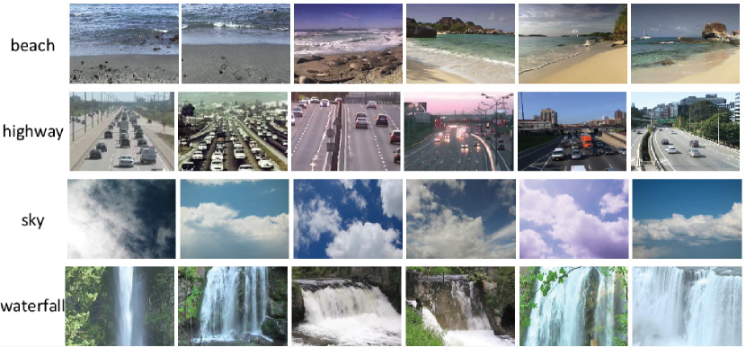
Figure 1: Sample images from dynamic scene data set YUPENN. Each row corresponds a category.

The remainder of the paper is organized as follows. We review the related studies in Section 2 and present our proposals in Section 3. We evaluate the proposed spatial and temporal TCoF schemes in Section 4 and finally we conclude this paper with a discussion in Section 5.

2 Related Work

In the literature, there are numerous approaches for dynamic texture and scene classification. While being closely relevant, dynamic texture classification [39, 27, 14, 40, 13, 12, 31, 6] and dynamic scene classification [37, 16, 11, 20, 15, 34] are usually considered separately as two different problems by far.

The research history of dynamic texture classification is much longer than that of the dynamic scene. The later, as far as we know, started since two dynamic scene data sets – Maryland Dynamic Scene data set “in the wild” [34] and York stabilized Dynamic Scene data set [27] – were released. Although there might not be a clear distinction in nature, the slight difference of dynamic texture from dynamic scene is that the frames in a video of dynamic texture consist of images with richer texture whereas the frames in a video of dynamic scene are a natural scene involving over time. In addition, having mentioned of the data sets, compared to dynamic textures which are usually stabilized videos, the dynamic scene data set might include some significant camera motions.

The critical challenges in categorizing the dynamic textures or scenes come from the wide range of variations around the naturally occurring phenomena. To overcome the difficulty, numerous methods for video representation have been proposed. Among them, Linear Dynamic System (LDS) based methods [14, 31, 1, 6], GIST based method [25], Local Binary Pattern (LBP) based methods [24, 40, 28, 29, 30], and wavelet based methods [12, 16, 17, 39] are the most widely used. LDS is a statistical generative model which captures the spatial appearance and dynamics in a video [14]. While LDS yields promising performance on viewpoint-invariant sequences, it performs poor on viewpoint-variant sequences [31, 1, 6]. Besides, it is also sensitive to illumination variations. GIST [25] represents the spatial envelope of an image (or a frame in video) holistically by Gabor filter. However GIST suffers from scale and rotation variations. Among LBP based methods, Local Binary Pattern on Three Orthogonal Planes (LBP-TOP) [40] is the most widely used. LBP-TOP describes a video by computing local binary pattern from three orthogonal planes ($xy$, $xt$ and $yt$) only. After LBP-TOP, several variants have been proposed, e.g., Local Ternary Pattern on Three Orthogonal Planes (LTP-TOP) [30], Weber Local Descriptor on Three Orthogonal Planes (WLD-TOP) [7], Local Phase Quantization on Three Orthogonal Planes (LQP-TOP) [30]. While LBP-TOP and its variants are effective at capturing spatial and temporal information and robust to illumination variations, they are suffering from camera motions. Recently, wavelet based methods are also proposed, e.g., Spatiotemporal Oriented Energy (SOE) [16], Wavelet Domain Multifractal Analysis (WDMA) [17], and Bag-of-Spacetime-Energy (BoSE)[16]. Combined with the Improved Fisher Vector (IFV) encoding strategy [26, 4], BoSE leads to the state-of-the-art performance on dynamic scene classification. However, the computational cost of BoSE is expensive due to slow feature extraction and quantization.

The aforementioned methods can be roughly divided into two categories: the global approaches and the local approaches. The global approaches extract features from each frame in a video sequence by treating each frame as a whole, e.g., LDS [14] and GIST [25]. While the global approaches describe the spatial layout information well, they suffer from the sensitivity to illumination variations, viewpoint changes, or scale and rotation variations. The local approaches construct a statistics (e.g., histogram) on a bunch of features extracted from local patches in each frame or local volumes in a video sequence, including LBP-TOP [40], LQP-TOP [30], BoSE [16], Bag of LDS [31]. While the local approaches are robustness to transformations (e.g., rotation, illumination), they suffer from the lack of spatial layout information which is important to represent a dynamic texture or dynamic scene.

In this paper, we attempt to leverage a deep structure with transferred knowledge from image domain to construct a robust and effective representation for dynamic textures and scenes. To be specific, we propose to use a pre-trained ConvNet – which has been trained on the large-scale image data set ImageNet [21], [33], [2] – as transferred (prior) knowledge, and then fine-tune the ConvNet with the frames in the videos of training set. Equipped with a trained ConvNet, we extract mid-level features from each frame in a video and represent a video by the concatenation of the first and the second order statistics over the mid-level features.

Compare to previous studies, our approach possesses the following advantages:

• Our approach represents a video with a two-level strategy. The deep structure used in the frame level is easier to train or even train-free, since we can adopt prior knowledge from image domain.

• The extracted frame-level features are robust to translations, small scale variations, partial rotations, and illumination variations.

• Our approach represents a video sequence by a concatenation of the first and the second order statistics of the frame-level features. This process is fast and effective.

In the next section, we will present the framework and two different implementations of our proposal.

3 Our Proposal: Transferred ConvNet Feature (TCoF)

Our TCoF scheme consists of three stages:

• Constructing a ConvNet with transferred knowledge from image domain;

• Extracting the mid-level feature with the ConvNet from each frame in a video;

• Forming the video-level representation by concatenating the calculated first and the second order statistics over the frame-level features.

3.1 Convolutional Neural Network with Transferred Knowledge for Extracting Frame-Level Features

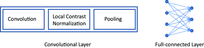
Figure 2: The typical structure of a ConvNet.

Notice that there are a lots of work in learning deep structures for classifying images. Among them, Convolutional Neural Networks (ConvNets) have been demonstrated to be extremely successful in computer vision [22, 21, 32, 18, 5, 2].

We show a typical structure of a ConvNet in Fig. 2. The ConvNet consists of two types of layers: convolutional layers and full-connected layers. The convolutional part, as shown in the left panel of Fig. 2, consists of three components – convolutions, Local Contrast Normalization (LCN), and pooling. Among the three components, the convolution block is compulsory, and LCN and the pooling are optional. The convolution components capture complex image structures. The LCN achieves invariance to illumination variations. The pooling component can not only yield partial invariance to scale variations and translations, but also reduce the complexity for the downstream layers. Due to sharing parameters which is motivated by the local reception field in biological vision system, the number of free parameters in the convolutional layer are significantly reduced. The full-connected layer, as shown in the right panel of Fig. 2, is the same as a multi-layer perception neural network.

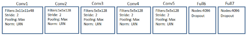
Figure 3: The architecture of the ConvNet used in our TCoF scheme.

In our TCoF framework, we use a ConvNet with five convolutional layers and two full-connected layers as shown in Fig. 3, which is the same as the most successful ConvNet implementation introduced by Krizhevsky et al. [21] and won the large-scale ImageNet contest, to extract the mid-level feature from each frame in a video. Note that we remove the final full-connected layer in the ConvNet introduced in [21].

As mentioned previously, training well a deep network like that in Fig.3 needs huge mount of training data and is quite expensive in computational demand. In our case, for dynamic texture or scene, the training data is limited. In stead of training a deep network from scratch, which is quite time-consuming, we propose to use the pre-trained ConvNet [21] as the initialization, and fine-tune the ConvNet with the frames in videos from training data if necessary. By using a good initialization, we virtually transfer miscellaneous prior knowledge from image domain (e.g., data set ImageNet) to the dynamic textures and scenes tasks.

3.2 Construct Video-Level Representation

Given a video sequence containing $N$ frames, the ConvNet yields $N$ ConvNet features. Note that as the input to the ConvNet in TCoF, we use each frame in a video subtracting an averaged image.

Denote $X$ as a set of the ConvNet features $\{\textbf{x}_{1},\textbf{x}_{2},...,\textbf{x}_{N}\}$ where $\textbf{x}_{i}\in R^{d}$ is the ConvNet feature extracted from $i$-th frame. We extract the first and the second order statistics on feature set $X$.

The first-order statistics of $X$ is the mean vector which is defined as follows:

$$\textbf{u}=\frac{1}{N}\sum_{i=1}^{N}\textbf{x}_{i},$$ (1)

where u captures the average behaviors of the $N$ ConvNet features which reflect the average characteristics in the video sequence.

The second-order statistics is the covariance matrix which is defined as follows:

$$\textbf{S}=\frac{1}{N}\sum_{i=1}^{N}(\textbf{x}_{i}-\textbf{u})(\textbf{x}_{i}-\textbf{u})^{\top},$$ (2)

where S describes the variation of the $N$ ConvNet features from the mean vector u and the correlations among different dimensions. The dimension of covariance feature is $\frac{d\times(d+1)}{2}$. When $d$ is large (e.g., $d=4096$), the dimension of the covariance feature is high. Instead, we propose to extract only the diagonal entries in S as the second-order feature, that is,

$$\textbf{v}=\text{diag}(\textbf{S}),$$ (3)

where $\text{diag}(\cdot)$ means to extract the diagonal entries of a matrix as a vector. The vector v is $d$-dimensional and captures the variations along each dimension in the ConvNet features.

Having calculated the first and the second order statistics, we form the video-level representation, TCoF, by concatenating u and v, i.e.,

$$\textbf{f}=\left[\begin{array}[]{c}\textbf{u}\\ \textbf{v}\\ \end{array}\right],$$ (4)

where the dimension of a TCoF representation is $2d$.

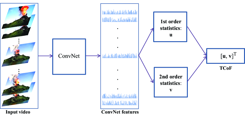
Figure 4: An illustration of our TCoF scheme.

For clarity, we illustrate the flowchart of constructing a TCoF representation for a video sequence in Fig. 4.

Remarks 1. Our proposed TCoF belongs to global approach. Since the spatial layout information can be captured well, we term the TCoF scheme described above as the spatial TCoF. Our proposed TCoF possesses the robustness to translations, small scale variations, partial rotations, and illumination variations owing to the ConvNet component. In addition, the process of extracting a TCoF vector is extremely fast since that the ConvNet adopt a so-called stride tactics and the second step in TCoF is to calculate the two statistics.

3.3 Modeling Temporal Information

While it is well accepted that dynamic information can enrich our understanding of the textures or scenes, modeling the dynamic information is difficult. Unlike the motion of rigid object, dynamic texture and scene are usually involving of non-rigid objects and thus the optical flow information seems relatively random.

In this paper, we propose to use the difference of the adjacent two frames in a short-time to capture the random-like micro-motion patterns. To be specific, we take the difference between the $(i+\tau)$-th and $i$-th frames as the input of the ConvNet component in TCoF scheme, where $\tau\in\{1,\cdots,N-1\}$ is an integer which corresponds to the resolution in time to capture the random-like micro-motion patterns. In practice, we set $\tau$ as a small integer, e.g., 1, 2 or 3.

Given a video sequence containing $N$ frames, the ConvNet produces $N-\tau$ temporal frame-level features. Then we extract the first and the second order statistics on the temporal ConvNet features to form a temporal TCoF for the input video, in the same way as the spatial TCoF in Section 3.2.

Remarks 2. The temporal TCoF differs from the spatial TCoF in the input of the ConvNet. In the spatial TCoF, we take each frame in a video subtracting a precalculated average image as input; whereas in the temporal TCoF we take the difference of two frames in a short-time and there is no need to subtract an average image.

Remarks 3. In our proposed TCoF, we treat the extracted $N$ ConvNet features as a set and ignore the sequential information among features. The rationale of this simplification comes from the property of dynamic textures and dynamic scenes. Note that the dynamic textures are visual processes of a group of particles with random motions, and dynamic scenes are places where natural events are occurring, the sequential information in these processes are relatively random and thus less critical. Experimental results in Section 4.3 support this point.

4 Experiments

In this section, we introduce the benchmark data sets, the baseline methods, and the implementation details, and then present the experimental evaluations of our approach.

4.1 Data Sets Description

DynTex [27] is a widely used dynamic texture data set, containing 656 videos with each sequence recorded in PAL format. The sequences in DynTex are divided into three data subsets – “Alpha”, “Beta” and “Gamma”: a) “Alpha” data subset contains 60 sequences which are equally divided into 3 categories: “sea”, “grass” and “trees”; b) “Beta” data subset consists 162 sequences which are grouped into 10 categories: “sea”, “grass”, “trees”, “flags”, “calm water”, “fountains”, “smoke”, “escalator”, “traffic”, and “rotation”; c) “Gamma” data subset is composed of 264 sequences which are grouped into 10 categories: “flowers”, “sea”, “trees without foliage”, “dense foliage”, “escalator”, “calm water”, “flags”, “grass”, “traffic” and “fountains”. Compared to “Alpha” and “Beta” data subsets, this data subset contains more complex image variations, e.g., scale, orientation, and etc. Sample frames from the three data subsets are shown in Fig. 5.

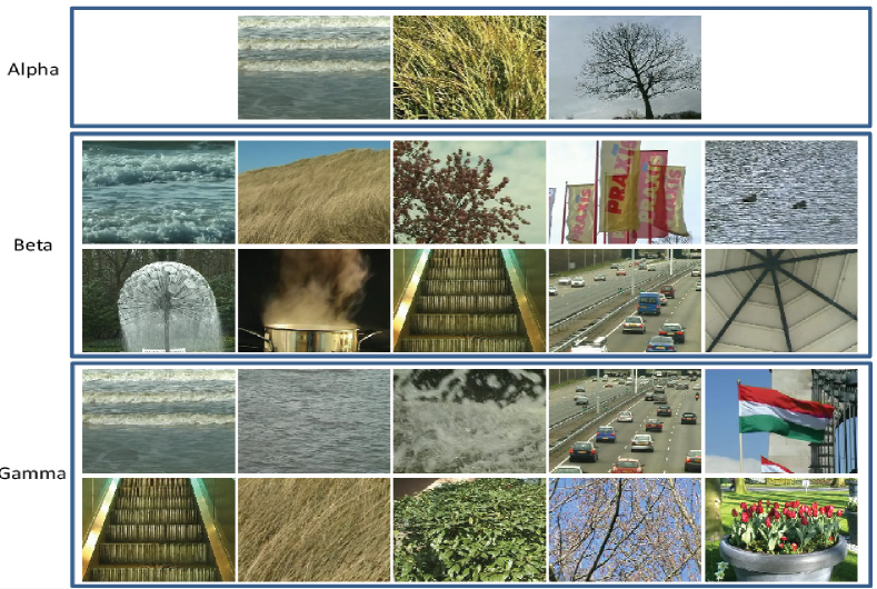
Figure 5: Sample frames from DynTex data set. The “Alpha” , “Beta”, and “Gamma” show the sample frames from each category in the data set.

YUPENN [11] is a “stabilized” dynamic scenes data set. This data set was introduced to emphasize scene-specific temporal information. YUPENN consists of fourteen dynamic scene categories with 30 color videos in each category. The sequences in YUPENN have significant variations, such as frame rate, scene appearance, scale, illumination, and camera viewpoint. Some sample frames are shown in Fig. 6.

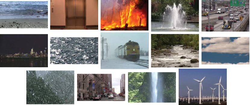
Figure 6: Samples from dynamic scene data set YUPENN. Each image corresponds to a category of video sequence.

Maryland [34] is a dynamic scene data set which was introduced firstly. It consists of 13 categories with 10 videos per category. The data set have large variations in illumination, frame rate, viewpoint, and scale. Besides, there are variations in resolution and camera dynamics. Some sample frames are shown in Fig. 7.

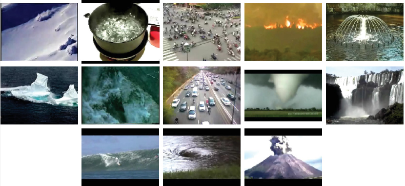
Figure 7: Sample frames from Maryland scenes data set.

4.2 Baselines and Implementation Details

Baselines We compare our proposed TCoF approach with the following state-of-the-art methods.

• GIST [25]: Holistic representation of the spatial envelope which is widely used in 2D static scene classification.

• Histogram of Flow (HOF) [23]: The HOF is an well-known descriptor in action recognition.

• Local Binary Pattern on Three Orthogonal Planes (LBP-TOP) [40]: The LBP-TOP is widely used in dynamic texture, dynamic facial expression, and dynamic facial micro-expression.

• Chaotic Dynamic Features (Chaos) [34].

• Slow Feature Analysis (SFA) [37].

• Synchrony Autoencoder (SAE) [20].

• Synchrony K-means (SK-means) [20].

• Complementary Spacetime Orientation (CSO) [15]: In CSO, the complementary spatial and temporal features are fused in a random forest framework.

• Bag of Spacetime Energy (BoSE) [16].

Implementation Details. In both the spatial TCoF (s-TCoF) and the temporal TCoF (t-TCoF), we resize the frame into $224\times 224$ and normalize both s-TCoF and t-TCoF with $L_{2}$-norm, respectively. For the combination of both the spatial and temporal TCoF, we take the concatenation of the two normalized s-TCoF and t-TCoF and denote it as st-TCoF. We do not use any data augmentation method. For our t-TCoF, we use $\tau=3$. We use the CAFFE toolbox [18] to extract the proposed TCoFs. Note that we take the weights in each layers but the final full connection layer in the well-trained ConvNet [21] as the initialization. And then, the whole ConvNet could be fine-tuned with the train data. While the fine-tuning stage is easier than training a ConvNet from scratch with random initialization, we observed that the improvement by the extra fine-tuning was minor. Thus we use the ConvNet without a further fine-tuning to extract the mid-level features. For LBP-TOP, we use the best performing setting of $\text{LBP-TOP}_{8,8,8,1,1,1}$, and the ${\chi}^{2}$ kernel. To fairly compare with previous methods, we test our approach and other baselines with both the nearest neighbor (NN) classifier and SVM classifier separately. In SVM, we use a linear SVM with Libsvm toolbox [3], in which the tradeoff parameter $C$ is fixed to 40 in all our experiments. Following the standard protocol, we use Leave-One-Out (LOO) cross-validation.

4.3 Evaluation of the Spatial and Temporal TCoFs

In this subsection, we evaluate systematically the influence of using the spatial and temporal TCoFs on DynTex, YUPENN, and Maryland data sets.

Effectiveness of the $s$-TCoF. Since that the s-TCoF features are constructed by accumulating all features in all frames, it is interesting to investigate the effect to the final performance of using different number of frames. To this end, we evaluate the s-TCoF using seven different settings: 1) using only the first frame in a video, 2) using the first $\frac{N}{8}$ frames in a video, 3) using the first $\frac{N}{4}$ frames in a video, 4) using the first $\frac{N}{2}$ frames in a video, and 5) using all $N$ frames in a video. Experimental results are shown in Table 1.

Table 1: Evaluation of the spatial TCoF (s-TCoF) by using different number of frames.

Datasets	1st	$\frac{N}{8}$	$\frac{N}{4}$	$\frac{N}{2}$	$N$
Alpha(NN)	100	100	100	100	100
Beta (NN)	98.77	99.38	99.38	98.77	99.38
Gamma(NN)	97.73	97.35	96.97	96.97	96.59
YUPENN(NN)	95.71	96.43	96.19	96.43	95.48
YUPENN(SVM)	96.90	96.90	96.90	97.14	96.90
Maryland(NN)	72.31	80.00	75.38	77.69	76.92
Maryland(SVM)	80.00	83.85	80.77	83.08	88.46

From Table 1, we can see that the spatial TCoF performs well by even using the first frame only, on DynTex and YUPENN data sets. This confirmed the effectiveness of the spatial TCoF scheme.

Table 2: Evaluating the performance of temporal TCoF (t-TCoF) as a function of parameter $\tau$.

Datasets	$\tau=1$	$\tau=2$	$\tau=3$	$\tau=4$	$\tau=5$
Alpha(NN)	98.33	96.67	96.67	96.67	96.67
Beta (NN)	97.53	96.91	97.53	97.53	97.53
Gamma(NN)	93.56	94.32	93.18	93.18	93.94
YUPENN(NN)	90.24	91.19	92.38	93.57	93.10
YUPENN(SVM)	94.52	96.19	96.67	96.90	97.14
Maryland(NN)	55.38	56.92	57.69	61.54	63.85
Maryland(SVM)	66.92	62.31	61.54	63.85	63.85

Effectiveness of the $t$-TCoF. Here, we conduct experiments to evaluate the influence of the parameter $\tau$. Experimental results are shown in Table 2. We observe from Table 2 that t-TCoF is not sensitive to the choice of $\tau$.

Comparison of s-TCof and t-TCoF. Note that almost all the results of s-TCoF in Table 1 outperform that of t-TCoF in Table 2. This suggest that s-TCoF is more effective than t-TCoF, since the randomness of the micro-motions in dynamic texture or natural dynamic scene makes the temporal information less critical. Nevertheless t-TCoF could provide complementary information to s-TCoF in some case that will be shown later.

4.4 Comparisons with the State-of-the-Art Methods

Dynamic Texture Classification on DynTex Data Set We conduct a set of experiments to compare our methods with LBP-TOP. Experimental results are shown in Table 3.

Table 3: Classification Results on DynTex dynamic texture data set. The performance of LBP-TOP is based on our implementation. All methods use NN classifier.

Datasets	LBP-TOP	s-TCoF	t-TCoF	st-TCoF
Alpha	96.67	100	96.67	98.33
Beta	85.80	99.38	97.53	98.15
Gamma	84.85	95.83	93.56	98.11

We observe from Table 3 that:

1. The s-TCoF performs the best on data subsets Alpha and Beta. This results confirm that the s-TCoF is effective for dynamic texture classification.

2. On Gamma subset, s-TCoF and t-TCoF significantly outperform LBP-TOP. Moreover by combining s-TCoF with t-TCoF, we achieve the best result. This result suggests that t-TCoF might provide complementary information to s-TCoF.

Dynamic Scene Classification on YUPENN. We compare our methods with the state-of-the-art methods, including CSO, GIST, SFA, SOE, SAE, BOSE, SK-means, and LBP-TOP, and the experimental results are presented in Table 4 and Table 5. We observe from Table 4 that:

1. The s-TCoF and t-TCoF both outperform the state-of-the-art methods. Note that YUPENN consist of stabilized videos. These results confirm that both s-TCoF and t-TCoF are effective for dynamic scene data in a stabilized setting.

2. The combination of the s-TCoF and t-TCoF, i.e., the st-TCoF, performs the best, in which reduce the error relatively over $30\%$. As shown is Table 5, s-TCoF and t-TCoF are complementary to each other on some categories, e.g., “Light Storm”, “Railway”, “Snowing”, and “Wind. Farm”.

Table 4: Classification results on scene data set YUPENN. The results of are taken from the corresponding papers. The performance of LBP-TOP is based on our implementation.

Methods	CSO	GIST	SFA	SAE	SOE	BoSE	SK-means	LBP-TOP	s-TCoF	t-TCoF	st-TCoF
NN	-	56	-	80.7	74	-	-	75.95	96.43	93.10	98.81
SVM	85.95	-	85.48	96.0	80.71	96.19	95.2	84.29	97.14	97.86	99.05

Table 5: Category-wise accuracy ($\%$) for different methods on dynamic scene data set YUPENN. All methods use linear SVM classifier. Our methods and LBP-TOP are based on our implementation. The other results are taken from [16].

Categories	HOF+	Chaos+	SOE	SFA	CSO	LBP-TOP	BoSE	s-TCoF	t-TCoF	st-TCoF
	GIST	GIST
Beach	87	30	93	93	100	87	100	97	97	97
Elevator	87	47	100	97	100	97	97	100	100	100
Forest Fire	63	17	67	70	83	87	93	100	97	100
Fountain	43	3	43	57	47	37	87	100	97	100
Highway	47	23	70	93	73	77	100	97	100	100
Light Storm	63	37	77	87	93	93	97	90	100	100
Ocean	97	43	100	100	90	97	100	100	100	100
Railway	83	7	80	93	93	80	100	97	100	100
Rush River	77	10	93	87	97	100	97	97	97	97
Sky-Clouds	87	47	83	93	100	93	97	100	97	100
Snowing	47	10	87	70	57	83	97	90	97	97
Street	77	17	90	97	97	93	100	100	97	100
Waterfall	47	10	63	73	77	90	83	93	93	97
Wind. Farm	53	17	83	87	93	67	100	100	100	100
Overall	68.33	22.86	80.71	85.48	85.95	84.29	96.19	97.14	97.86	99.05

Dynamic Scene Classification on dynamic scene data set Maryland. We present the comparison of our methods with the state-of-the-art methods in Table 6. We observe from Table 6 that:

1. The s-TCoF significantly outperforms the other methods. This suggests that the spatial information is extremely important for scene understanding.

2. The results of t-TCoF are much worse than s-TCoF. This might be due to the significant camera motions in this data set.

Table 6: Classification results on scene data set Maryland. The results of are taken from the corresponding papers. The performance of LBP-TOP is based on our implementation.

Methods	CSO	SFA	SOE	BoSE	LBP-TOP	s-TCoF	t-TCoF	st-TCoF
NN	-	-	-	-	31.54	74.62	58.46	74.62
SVM	67.69	60	43.1	77.69	39.23	88.46	66.15	88.46

4.5 Further Investigations and Remarks

Data Visualization. To show the discriminative power of the proposed approach, we use t-Stochastic Neighbor Embedding (t-SNE) [38] to visualize the data distributions of the dynamic scene data sets YUPENN and Maryland. Results are shown in Fig. 8 and Fig. 9, respectively. We observe from Fig. 8 and Fig. 9 that s-TCoF, t-TCoF, and st-TCoF yield distinct separations between categories. These results reveal the effectiveness of our proposed TCoF approach vividly.

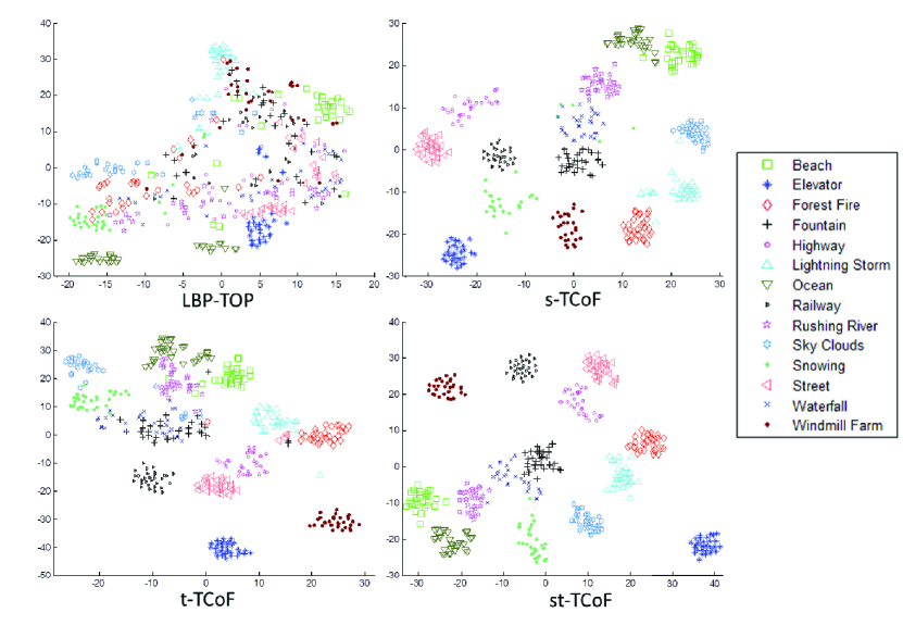
Figure 8: Data visualization of LBP-TOP, s-TCoF, t-TCoF, and st-TCoF on YUPENN dynamic scene data set. Each point in the figure corresponds to a video sequence.

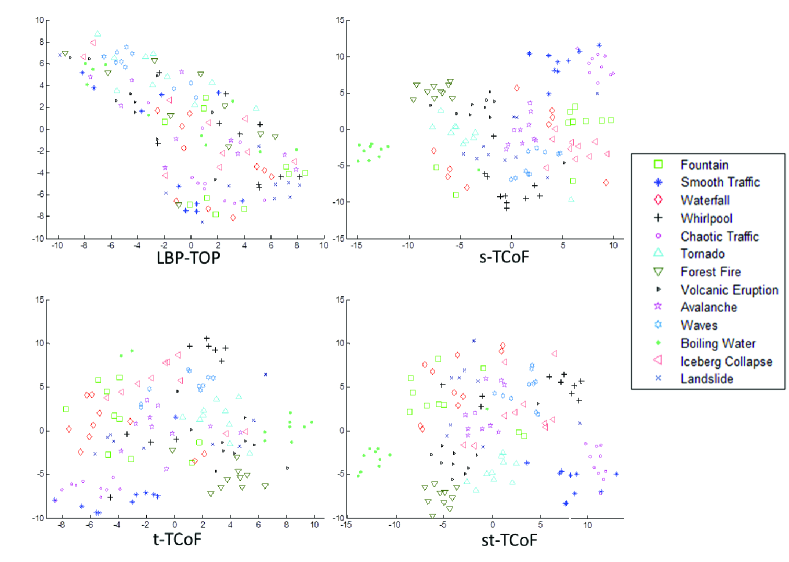
Figure 9: Data visualization of LBP-TOP, s-TCoF, t-TCoF, and st-TCoF on Maryland dynamic scene data set. Each point in the figure corresponds to a video sequence.

Remarks. Note that in our TCoF schemes, we treat the frames in a video as orderless images and extract mid-level features with a ConvNet. By doing so, the sequential information among features is ignored. The superior experimental results suggest that such a simplification is harmless. The sequential information in these processes contributes less (or not at all) discriminativeness, because that the dynamic textures can be viewed as visual processes of a group of particles with random motions, and the dynamic scenes are places where natural events are occurring. The effectiveness underlying our proposed TCoF approach for dynamic texture and scene classification is due to the following aspects:

• Rich filters’ combination built on color channels in ConvNet describes richer structures and color information. The filters that are built on different image patches capture stronger and richer structures compared to the hand-crafted features.

• ConvNet makes the extracted features robust to sorts of image transformations due to the max-pooling and LCN components. Specifically the max-pooling tactics makes ConvNet robust to translations, small scale variations, and partial rotations, and LCN makes ConvNet robust to illumination variations.

• The first and the second order statistics capture enough information over the mid-level features.

• When the video sequences are stabilized, the t-TCoF might provide complementary information to the s-TCoF.

5 Conclusion and Discussion

We have proposed a robust and effective feature extraction approach for dynamic texture and scene classification, termed as Transferred ConvNet Features (TCoF), which was built on the first and the second order statistics of the mid-level features extracted by a ConvNet with transferred knowledge from image domain. We have investigated two different implementations of the TCoF scheme, i.e., the spatial TCoF and the temporal TCoF. We have evaluated systematically the proposed approaches on three benchmark data sets and confirmed that: a) the proposed spatial TCoF was effective, and b) the temporal TCoF could provides complementary information when the camera is stabilized.

Unlike images, representing a video sequence needs to consider the following aspects:

1. To depict the spatial information. In most cases, we can recognize the dynamic textures and scenes from a single frame in a video. Thus, extracting the spatial information of each frame in a video might be an effective way to represent the dynamic textures or scenes.

2. To capture the temporal information. In dynamic textures or scenes, there are some specific micro-motion patterns. Capturing these micro-motion patterns might help to better understand the dynamic textures or scenes.

3. To fuse the spatial and temporal information. When the spatial and temporal information are complementary, combining both of them might boost the recognition performance.

Different from the rigid or semi-rigid objects (e.g., actions), the dynamics of texture and scene are relatively random and non-directional. Whereas the temporal information might be the most important cue in action recognition [23, 19], our investigation in this paper suggests that the sequential information in dynamic textures or scenes is not that critical for classification.

References

- Afsari et al. [2012] Afsari, B., Chaudhry, R., Ravichandran, A., Vidal, R., 2012. Group action induced distances for averaging and clustering linear dynamical systems with applications to the analysis of dynamic scenes. In: IEEE Conference on Computer Vision and Pattern Recognition (CVPR). IEEE, pp. 2208–2215.
- Azizpour et al. [2014] Azizpour, H., Razavian, A. S., Sullivan, J., Maki, A., Carlsson, S., 2014. From generic to specific deep representations for visual recognition. arXiv preprint arXiv:1406.5774.
- Chang and Lin [2011] Chang, C.-C., Lin, C.-J., 2011. Libsvm: a library for support vector machines. ACM Transactions on Intelligent Systems and Technology (TIST) 2 (3), 27.
- Chatfield et al. [2011] Chatfield, K., Lempitsky, V., Vedaldi, A., Zisserman, A., 2011. The devil is in the details: an evaluation of recent feature encoding methods. In: British Machine Vision Conference.
- Chatfield et al. [2014] Chatfield, K., Simonyan, K., Vedaldi, A., Zisserman, A., 2014. Return of the devil in the details: Delving deep into convolutional nets. In: British Machine Vision Conference.
- Chaudhry et al. [2013] Chaudhry, R., Hager, G., Vidal, R., 2013. Dynamic template tracking and recognition. International Journal of Computer Vision 105 (1), 19–48.
- Chen et al. [2013] Chen, J., Zhao, G., Salo, M., Rahtu, E., Pietikainen, M., 2013. Automatic dynamic texture segmentation using local descriptors and optical flow. IEEE Transactions on Image Processing 22 (1), 326–339.
- Collobert and Weston [2008] Collobert, R., Weston, J., 2008. A unified architecture for natural language processing: Deep neural networks with multitask learning. In: Proceedings of the 25th International Conference on Machine Learning. ACM, pp. 160–167.
- Collobert et al. [2011] Collobert, R., Weston, J., Bottou, L., Karlen, M., Kavukcuoglu, K., Kuksa, P., 2011. Natural language processing (almost) from scratch. The Journal of Machine Learning Research 12, 2493–2537.
- Deng et al. [2013] Deng, L., Li, J., Huang, J.-T., Yao, K., Yu, D., Seide, F., Seltzer, M., Zweig, G., He, X., Williams, J., et al., 2013. Recent advances in deep learning for speech research at microsoft. In: IEEE International Conference on Acoustics, Speech and Signal Processing (ICASSP). IEEE, pp. 8604–8608.
- Derpanis et al. [2012] Derpanis, K. G., Lecce, M., Daniilidis, K., Wildes, R. P., 2012. Dynamic scene understanding: The role of orientation features in space and time in scene classification. In: IEEE Conference on Computer Vision and Pattern Recognition (CVPR). IEEE, pp. 1306–1313.
- Derpanis and Wildes [2010] Derpanis, K. G., Wildes, R. P., 2010. Dynamic texture recognition based on distributions of spacetime oriented structure. In: IEEE Conference on Computer Vision and Pattern Recognition (CVPR). IEEE, pp. 191–198.
- Derpanis and Wildes [2012] Derpanis, K. G., Wildes, R. P., 2012. Spacetime texture representation and recognition based on a spatiotemporal orientation analysis. IEEE Transactions on Pattern Analysis and Machine Intelligence 34 (6), 1193–1205.
- Doretto et al. [2003] Doretto, G., Chiuso, A., Wu, Y. N., Soatto, S., 2003. Dynamic textures. International Journal of Computer Vision 51 (2), 91–109.
- Feichtenhofer et al. [2013] Feichtenhofer, C., Pinz, A., Wildes, R. P., 2013. Spacetime forests with complementary features for dynamic scene recognition. British Machine Vision Conference.
- Feichtenhofer et al. [2014] Feichtenhofer, C., Pinz, A., Wildes, R. P., 2014. Bags of spacetime energies for dynamic scene recognition. In: IEEE Conference on Computer Vision and Pattern Recognition (CVPR). IEEE.
- Ji et al. [2013] Ji, H., Yang, X., Ling, H., Xu, Y., 2013. Wavelet domain multifractal analysis for static and dynamic texture classification. IEEE Transactions on Image Processing 22 (1), 286–299.
- Jia [2013] Jia, Y., 2013. Caffe: An open source convolutional architecture for fast feature embedding. http://caffe.berkeleyvision.org.
- Karpathy et al. [2014] Karpathy, A., Toderici, G., Shetty, S., Leung, T., Sukthankar, R., Fei-Fei, L., 2014. Large-scale video classification with convolutional neural networks. In: IEEE Conference on Computer Vision and Pattern Recognition (CVPR).
- Konda et al. [2013] Konda, K., Memisevic, R., Michalski, V., 2013. Learning to encode motion using spatio-temporal synchrony. In: International Conference on Learning Representations.
- Krizhevsky et al. [2012] Krizhevsky, A., Sutskever, I., Hinton, G. E., 2012. Imagenet classification with deep convolutional neural networks. In: Advances in Neural Information Processing Systems. pp. 1097–1105.
- LeCun et al. [1998] LeCun, Y., Bottou, L., Bengio, Y., Haffner, P., 1998. Gradient-based learning applied to document recognition. Proceedings of the IEEE 86 (11), 2278–2324.
- Marszalek et al. [2009] Marszalek, M., Laptev, I., Schmid, C., 2009. Actions in context. In: IEEE Conference on Computer Vision and Pattern Recognition. IEEE, pp. 2929–2936.
- Ojala et al. [2002] Ojala, T., Pietikainen, M., Maenpaa, T., 2002. Multiresolution gray-scale and rotation invariant texture classification with local binary patterns. IEEE Transactions on Pattern Analysis and Machine Intelligence 24 (7), 971–987.
- Oliva and Torralba [2001] Oliva, A., Torralba, A., 2001. Modeling the shape of the scene: A holistic representation of the spatial envelope. International Journal of Computer Vision 42 (3), 145–175.
- Perronnin et al. [2010] Perronnin, F., Sánchez, J., Mensink, T., 2010. Improving the fisher kernel for large-scale image classification. In: European Conference on Computer Vision. Springer, pp. 143–156.
- Péteri et al. [2010] Péteri, R., Fazekas, S., Huiskes, M. J., 2010. Dyntex: A comprehensive database of dynamic textures. Pattern Recognition Letters 31 (12), 1627–1632.
- Pietikäinen et al. [2011] Pietikäinen, M., Hadid, A., Zhao, G., Ahonen, T., 2011. Computer vision using local binary patterns. Vol. 40. Springer.
- Qi et al. [2012] Qi, X., Xiao, R., Guo, J., Zhang, L., 2012. Pairwise rotation invariant co-occurrence local binary pattern. In: European Conference on Computer Vision. Springer, pp. 158–171.
- Rahtu et al. [2012] Rahtu, E., Heikkilä, J., Ojansivu, V., Ahonen, T., 2012. Local phase quantization for blur-insensitive image analysis. Image and Vision Computing 30 (8), 501–512.
- Ravichandran et al. [2013] Ravichandran, A., Chaudhry, R., Vidal, R., 2013. Categorizing dynamic textures using a bag of dynamical systems. IEEE Transactions on Pattern Analysis and Machine Intelligence 35 (2), 342–353.
- Sermanet et al. [2013] Sermanet, P., Eigen, D., Zhang, X., Mathieu, M., Fergus, R., LeCun, Y., 2013. Overfeat: Integrated recognition, localization and detection using convolutional networks. arXiv preprint arXiv:1312.6229.
- Sharif Razavian et al. [2014] Sharif Razavian, A., Azizpour, H., Sullivan, J., Carlsson, S., 2014. Cnn features off-the-shelf: an astounding baseline for recognition. arXiv preprint arXiv:1403.6382.
- Shroff et al. [2010] Shroff, N., Turaga, P., Chellappa, R., 2010. Moving vistas: Exploiting motion for describing scenes. In: IEEE Conference on Computer Vision and Pattern Recognition (CVPR). IEEE, pp. 1911–1918.
- Sun et al. [2014a] Sun, Y., Wang, X., Tang, X., 2014a. Deep learning face representation by joint identification-verification. arXiv preprint arXiv:1406.4773.
- Sun et al. [2014b] Sun, Y., Wang, X., Tang, X., 2014b. Deep learning face representation from predicting 10,000 classes. In: The IEEE Conference on Computer Vision and Pattern Recognition (CVPR).
- Theriault et al. [2013] Theriault, C., Thome, N., Cord, M., 2013. Dynamic scene classification: Learning motion descriptors with slow features analysis. In: IEEE Conference on Computer Vision and Pattern Recognition (CVPR). IEEE, pp. 2603–2610.
- Van der Maaten and Hinton [2008] Van der Maaten, L., Hinton, G., 2008. Visualizing data using t-sne. Journal of Machine Learning Research 9 (2579-2605), 85.
- Xu et al. [2011] Xu, Y., Quan, Y., Ling, H., Ji, H., 2011. Dynamic texture classification using dynamic fractal analysis. In: IEEE International Conference on International Conference on Computer Vision (ICCV). IEEE, pp. 1219–1226.
- Zhao and Pietikainen [2007] Zhao, G., Pietikainen, M., 2007. Dynamic texture recognition using local binary patterns with an application to facial expressions. IEEE Transactions on Pattern Analysis and Machine Intelligence 29 (6), 915–928.