The lowest hidden charmed tetraquark state from QCD sum rules

Zhi-Gang Wang 111E-mail: zgwang@aliyun.com.

Department of Physics, North China Electric Power University, Baoding 071003, P. R. China

Abstract

In this article, we study the $S\bar{S}$ type scalar tetraquark state $cq\bar{c}\bar{q}$ in details with the QCD sum rules by calculating the contributions of the vacuum condensates up to dimension-10 in the operator product expansion, and obtain the value $M_{Z_{c}}=\left(3.82^{+0.08}_{-0.08}\right)\,\rm{GeV}$, which is the lowest mass for the hidden charmed tetraquark states from the QCD sum rules. Furthermore, we calculate the hadronic coupling constants $G_{Z_{c}\eta_{c}\pi}$ and $G_{Z_{c}DD}$ with the three-point QCD sum rules, then study the strong decays $Z_{c}\to\eta_{c}\pi\,,\,DD$, and observe that the total width $\Gamma_{Z_{c}}\approx 21\,\rm{MeV}$. The present predictions can be confronted with the experimental data in the futures at the BESIII, LHCb and Belle-II.

PACS number: 12.39.Mk, 12.38.Lg

Key words: Tetraquark state, QCD sum rules

1 Introduction

The scattering amplitude for one-gluon exchange in an $SU(N_{c})$ gauge theory is proportional to

$\displaystyle t^{a}_{ki}t^{a}_{lj}$ $\displaystyle=$ $\displaystyle-\frac{N_{c}+1}{4N_{c}}(\delta_{jk}\delta_{il}-\delta_{ik}\delta_{jl})+\frac{N_{c}-1}{4N_{c}}(\delta_{jk}\delta_{il}+\delta_{ik}\delta_{jl})\,,$ (1)

where the $t^{a}$ is the generator of the gauge group, and the $i,j$ and $k,l$ are the color indexes of the two quarks in the incoming and outgoing channels respectively. For $N_{c}=3$, the negative sign in front of the antisymmetric antitriplet indicates the interaction is attractive and favors the formation of the diquark states in the color antitriplet, while the positive sign in front of the symmetric sextet indicates the interaction is repulsive and disfavors the formation of the diquark states in the color sextet [1].

The antitriplet diquark states have five Dirac tensor structures, scalar $C\gamma_{5}$, pseudoscalar $C$, vector $C\gamma_{\mu}\gamma_{5}$, axial vector $C\gamma_{\mu}$ and tensor $C\sigma_{\mu\nu}$. The structures $C\gamma_{\mu}$ and $C\sigma_{\mu\nu}$ are symmetric, the structures $C\gamma_{5}$, $C$ and $C\gamma_{\mu}\gamma_{5}$ are antisymmetric. The attractive interactions of one-gluon exchange favor formation of the diquarks in color antitriplet $\overline{3}_{c}$, flavor antitriplet $\overline{3}_{f}$ and spin singlet $1_{s}$ (or flavor sextet $6_{f}$ and spin triplet $3_{s}$) [2, 3], so the favored configurations are the scalar and axial-vector diquark states. The scalar ($S$) and axial-vector ($A$) heavy-light diquark states have almost degenerate masses from the QCD sum rules [4, 5]. In Refs.[6, 7], we take the $C\gamma_{5}-C\gamma_{5}$, $C\gamma_{\mu}-C\gamma^{\mu}$, $C\gamma_{\mu}\gamma_{5}-C\gamma^{\mu}\gamma_{5}$ type interpolating currents to study the masses of the scalar tetraquark states in a systematic way using the QCD sum rules, and observe that the $S\bar{S}$ and $A\bar{A}$ type scalar tetraquark states have almost degenerate masses, about $4.36\,\rm{GeV}$, which is much larger than that from the phenomenological models [8, 9, 10].

In Ref.[8], Ebert, Faustov and Galkin calculate the masses of the excited heavy tetraquarks with hidden charm within the relativistic diquark-antidiquark picture based on the quasipotential approach, and obtain the values $M_{J=0}=3.852\,\rm{GeV}$ and $3.812\,\rm{GeV}$ for the $A\bar{A}$ and $S\bar{S}$ type scalar tetraquark states $cq\bar{c}\bar{q}$, respectively. While L. Maiani et al obtain the values $M_{J=0}=3.832\,\rm{GeV}$ and $3.723\,\rm{GeV}$ for the $A\bar{A}$ and $S\bar{S}$ type scalar tetraquark states $cq\bar{c}\bar{q}$ respectively in the type-I diquark-antidiquark model [9], and $M_{J=0}=4.000\,\rm{GeV}$ and $3.770\,\rm{GeV}$ for the $A\bar{A}$ and $S\bar{S}$ type scalar tetraquark states $cq\bar{c}\bar{q}$ respectively in the type-II diquark-antidiquark model [10]. In those model-dependent studies, the masses of the $A\bar{A}$-type scalar tetraquark states are larger than that of the $S\bar{S}$ type scalar tetraquark states.

In Refs.[11, 12, 13, 14, 15, 16], we explore the energy scale dependence of the hidden charmed (bottom) tetraquark states and molecular states in details for the first time, and suggest a formula

$\displaystyle\mu$ $\displaystyle=$ $\displaystyle\sqrt{M^{2}_{X/Y/Z}-(2{\mathbb{M}}_{Q})^{2}}\,,$ (2)

with the effective heavy $Q$-quark mass ${\mathbb{M}}_{Q}$ to determine the energy scales of the QCD spectral densities in the QCD sum rules, which works well. According to the formula, the energy scale $\mu=1\,\rm{GeV}$ taken in Refs.[6, 7] is too low to result in robust predictions.

In Ref.[14], we choose the $C\gamma_{\mu}-C\gamma_{\nu}$ type interpolating currents to study the $A\bar{A}$-type scalar, axial-vector and tensor tetraquark states in details with the QCD sum rules. The predicted masses of the axial-vector and tensor tetraquark states favor assigning the $Z_{c}(4020)$ and $Z_{c}(4025)$ as the $J^{PC}=1^{+-}$ or $2^{++}$ diquark-antidiquark type tetraquark states. While there are no experimental candidates to match the predicted mass of the scalar tetraquark state $M_{J=0}=\left(3.85^{+0.15}_{-0.09}\right)\,\rm{GeV}$. The value is consistent with the prediction $M_{J=0}=3.852\,\rm{GeV}$ based on the quasipotential approach [8], while the upper bound reaches the prediction $M_{J=0}=4.000\,\rm{GeV}$ based on the type-II diquark-antidiquark model [10]. According to Refs.[8, 9, 10], the $S\bar{S}$-type scalar tetraquark states have smaller masses than that of the corresponding $A\bar{A}$-type scalar tetraquark states. It is interesting to see whether or not such conclusion survives when confronted with the QCD sum rules. In Refs.[11, 12, 13], we observe that the masses of the $S\bar{A}$ or $A\bar{S}$ type axial-vector tetraquark states are larger than that of the $A\bar{A}$ type scalar tetraquark states. So the $S\bar{S}$ scalar tetraquark state maybe the lowest tetraquark state.

In this article, we study the scalar $S\bar{S}$-type hidden charmed tetraquark state (thereafter we will denote it as $Z_{c}$) by calculating the contributions of the vacuum condensates up to dimension-10, and try to obtain the lowest mass based on the QCD sum rules. Furthermore, we calculate the hadronic coupling constants $G_{Z_{c}\eta_{c}\pi}$ and $G_{Z_{c}DD}$ with the three-point QCD sum rules, then study the strong decays $Z_{c}\to\eta_{c}\pi\,,\,DD$.

The article is arranged as follows: we derive the QCD sum rules for the mass and pole residue of the scalar tetraquark state $Z_{c}$ and for the hadronic coupling constants $G_{Z_{c}\eta_{c}\pi}$ and $G_{Z_{c}DD}$ in section 2; in section 3, we present the numerical results and discussions; section 4 is reserved for our conclusion.

2 QCD sum rules for the scalar tetraquark state

In the following, we write down the two-point correlation function $\Pi(p)$ in the QCD sum rules,

$\displaystyle\Pi(p)$ $\displaystyle=$ $\displaystyle i\int d^{4}xe^{ip\cdot x}\langle 0|T\left\{J(x)J^{\dagger}(0)\right\}|0\rangle\,,$ (3)
$\displaystyle J(x)$ $\displaystyle=$ $\displaystyle\epsilon^{ijk}\epsilon^{imn}u^{j}(x)C\gamma_{5}c^{k}(x)\bar{d}^{m}(x)\gamma_{5}C\bar{c}^{n}(x)\,,$ (4)

where the $i$, $j$, $k$, $m$, $n$ are color indexes, the $C$ is the charge conjugation matrix.

At the hadronic side, we can insert a complete set of intermediate hadronic states with the same quantum numbers as the current operator $J(x)$ into the correlation function $\Pi(p)$ to obtain the hadronic representation [17, 18, 19]. After isolating the ground state contribution of the scalar tetraquark state, we get the following result,

$\displaystyle\Pi(p)$ $\displaystyle=$ $\displaystyle\frac{\lambda_{Z_{c}}^{2}}{M_{Z_{c}}^{2}-p^{2}}+\cdots\,\,,$ (5)

where the pole residue $\lambda_{Z_{c}}$ is defined by $\langle 0|J(0)|Z(p)\rangle=\lambda_{Z_{c}}$ .

In the following, we briefly outline the operator product expansion for the correlation function $\Pi(p)$ in perturbative QCD. We contract the $u$, $d$ and $c$ quark fields in the correlation function $\Pi(p)$ with Wick theorem, and obtain the result:

$\displaystyle\Pi(p)$ $\displaystyle=$ $\displaystyle i\epsilon^{ijk}\epsilon^{imn}\epsilon^{i^{\prime}j^{\prime}k^{\prime}}\epsilon^{i^{\prime}m^{\prime}n^{\prime}}\int d^{4}xe^{ip\cdot x}$ (6)
$\displaystyle{\rm Tr}\left[\gamma_{5}C^{kk^{\prime}}(x)\gamma_{5}CU^{jj^{\prime}T}(x)C\right]{\rm Tr}\left[\gamma_{5}C^{n^{\prime}n}(-x)\gamma_{5}CD^{m^{\prime}mT}(-x)C\right]\,,$

where the $U_{ij}(x)$, $D_{ij}(x)$ and $C_{ij}(x)$ are the full $u$, $d$ and $c$ quark propagators respectively (the $U_{ij}(x)$ and $D_{ij}(x)$ can be written as $S_{ij}(x)$ for simplicity),

$\displaystyle S_{ij}(x)$ $\displaystyle=$ i​δi​j​​x2​π2​x4βˆ’Ξ΄i​jβ€‹βŸ¨q¯​q⟩12βˆ’Ξ΄i​j​x2β€‹βŸ¨q¯​gs​σ​G​q⟩192βˆ’i​gs​Gα​βa​ti​ja​(​x​σα​β+σα​β​​x)32​π2​x2βˆ’i​δi​j​x2​​x​gs2β€‹βŸ¨q¯​q⟩27776𝑖subscript𝛿𝑖𝑗π‘₯2superscriptπœ‹2superscriptπ‘₯4subscript𝛿𝑖𝑗delimited-βŸ¨βŸ©Β―π‘žπ‘ž12subscript𝛿𝑖𝑗superscriptπ‘₯2delimited-βŸ¨βŸ©Β―π‘žsubscriptπ‘”π‘ πœŽπΊπ‘ž192𝑖subscript𝑔𝑠subscriptsuperscriptπΊπ‘Žπ›Όπ›½subscriptsuperscriptπ‘‘π‘Žπ‘–π‘—π‘₯superscriptπœŽπ›Όπ›½superscriptπœŽπ›Όπ›½π‘₯32superscriptπœ‹2superscriptπ‘₯2𝑖subscript𝛿𝑖𝑗superscriptπ‘₯2π‘₯superscriptsubscript𝑔𝑠2superscriptdelimited-βŸ¨βŸ©Β―π‘žπ‘ž27776\displaystyle\frac{i\delta_{ij}\!\not\!{x}}{2\pi^{2}x^{4}}-\frac{\delta_{ij}\langle\bar{q}q\rangle}{12}-\frac{\delta_{ij}x^{2}\langle\bar{q}g_{s}\sigma Gq\rangle}{192}-\frac{ig_{s}G^{a}_{\alpha\beta}t^{a}_{ij}(\!\not\!{x}\sigma^{\alpha\beta}+\sigma^{\alpha\beta}\!\not\!{x})}{32\pi^{2}x^{2}}-\frac{i\delta_{ij}x^{2}\!\not\!{x}g_{s}^{2}\langle\bar{q}q\rangle^{2}}{7776} (7)
$\displaystyle-\frac{\delta_{ij}x^{4}\langle\bar{q}q\rangle\langle g_{s}^{2}GG\rangle}{27648}-\frac{1}{8}\langle\bar{q}_{j}\sigma^{\mu\nu}q_{i}\rangle\sigma_{\mu\nu}-\frac{1}{4}\langle\bar{q}_{j}\gamma^{\mu}q_{i}\rangle\gamma_{\mu}+\cdots\,,$
$\displaystyle C_{ij}(x)$ $\displaystyle=$ $\displaystyle\frac{i}{(2\pi)^{4}}\int d^{4}ke^{-ik\cdot x}\left\{\frac{\delta_{ij}}{\!\not\!{k}-m_{c}}-\frac{g_{s}G^{n}_{\alpha\beta}t^{n}_{ij}}{4}\frac{\sigma^{\alpha\beta}(\!\not\!{k}+m_{c})+(\!\not\!{k}+m_{c})\sigma^{\alpha\beta}}{(k^{2}-m_{c}^{2})^{2}}\right.$
$\displaystyle\left.+\frac{g_{s}D_{\alpha}G^{n}_{\beta\lambda}t^{n}_{ij}(f^{\lambda\beta\alpha}+f^{\lambda\alpha\beta})}{3(k^{2}-m_{c}^{2})^{4}}-\frac{g_{s}^{2}(t^{a}t^{b})_{ij}G^{a}_{\alpha\beta}G^{b}_{\mu\nu}(f^{\alpha\beta\mu\nu}+f^{\alpha\mu\beta\nu}+f^{\alpha\mu\nu\beta})}{4(k^{2}-m_{c}^{2})^{5}}+\cdots\right\}\,,$
$\displaystyle f^{\lambda\alpha\beta}$ $\displaystyle=$ $\displaystyle(\!\not\!{k}+m_{c})\gamma^{\lambda}(\!\not\!{k}+m_{c})\gamma^{\alpha}(\!\not\!{k}+m_{c})\gamma^{\beta}(\!\not\!{k}+m_{c})\,,$
$\displaystyle f^{\alpha\beta\mu\nu}$ $\displaystyle=$ $\displaystyle(\!\not\!{k}+m_{c})\gamma^{\alpha}(\!\not\!{k}+m_{c})\gamma^{\beta}(\!\not\!{k}+m_{c})\gamma^{\mu}(\!\not\!{k}+m_{c})\gamma^{\nu}(\!\not\!{k}+m_{c})\,,$ (8)

and $t^{n}=\frac{\lambda^{n}}{2}$, the $\lambda^{n}$ is the Gell-Mann matrix, $D_{\alpha}=\partial_{\alpha}-ig_{s}G^{n}_{\alpha}t^{n}$ [19], then compute the integrals both in the coordinate and momentum spaces to obtain the correlation function $\Pi(p)$ therefore the QCD spectral density. In Eq.(7), we retain the terms $\langle\bar{q}_{j}\sigma_{\mu\nu}q_{i}\rangle$ and $\langle\bar{q}_{j}\gamma_{\mu}q_{i}\rangle$ originate from the Fierz re-arrangement of the $\langle q_{i}\bar{q}_{j}\rangle$ to absorb the gluons emitted from the heavy quark lines so as to extract the mixed condensate and four-quark condensate ⟨q¯​gs​σ​G​q⟩delimited-βŸ¨βŸ©Β―π‘žsubscriptπ‘”π‘ πœŽπΊπ‘ž\langle\bar{q}g_{s}\sigma Gq\rangle and $g_{s}^{2}\langle\bar{q}q\rangle^{2}$, respectively.

Once the analytical expression is obtained, we can take the quark-hadron duality below the continuum threshold $s_{0}$ and perform Borel transform with respect to the variable $P^{2}=-p^{2}$ to obtain the following QCD sum rule:

Ξ»Zc2​exp⁑(βˆ’MZc2T2)=∫4​mc2s0𝑑s​ρ​(s)​exp⁑(βˆ’sT2),subscriptsuperscriptπœ†2subscript𝑍𝑐subscriptsuperscript𝑀2subscript𝑍𝑐superscript𝑇2superscriptsubscript4superscriptsubscriptπ‘šπ‘2subscript𝑠0differential-dπ‘ πœŒπ‘ π‘ superscript𝑇2\displaystyle\lambda^{2}_{Z_{c}}\,\exp\left(-\frac{M^{2}_{Z_{c}}}{T^{2}}\right)=\int_{4m_{c}^{2}}^{s_{0}}ds\,\rho(s)\,\exp\left(-\frac{s}{T^{2}}\right)\,, (9)

where

ρ​(s)πœŒπ‘ \displaystyle\rho(s) $\displaystyle=$ $\displaystyle\rho_{0}(s)+\rho_{3}(s)+\rho_{4}(s)+\rho_{5}(s)+\rho_{6}(s)+\rho_{7}(s)+\rho_{8}(s)+\rho_{10}(s)\,,$ (10)
$\displaystyle\rho_{0}(s)$ $\displaystyle=$ $\displaystyle\frac{1}{512\pi^{6}}\int_{y_{i}}^{y_{f}}dy\int_{z_{i}}^{1-y}dz\,yz\,(1-y-z)^{3}\left(s-\overline{m}_{c}^{2}\right)^{2}\left(7s^{2}-6s\overline{m}_{c}^{2}+\overline{m}_{c}^{4}\right)\,,$ (11)
$\displaystyle\rho_{3}(s)$ $\displaystyle=$ $\displaystyle-\frac{m_{c}\langle\bar{q}q\rangle}{16\pi^{4}}\int_{y_{i}}^{y_{f}}dy\int_{z_{i}}^{1-y}dz\,(y+z)(1-y-z)\left(s-\overline{m}_{c}^{2}\right)\left(2s-\overline{m}_{c}^{2}\right)\,,$ (12)
$\displaystyle\rho_{4}(s)$ $\displaystyle=$ βˆ’mc2384​π4β€‹βŸ¨Ξ±s​G​GΟ€βŸ©β€‹βˆ«yiyf𝑑yβ€‹βˆ«zi1βˆ’y𝑑z​(zy2+yz2)​(1βˆ’yβˆ’z)3superscriptsubscriptπ‘šπ‘2384superscriptπœ‹4delimited-⟨⟩subscriptπ›Όπ‘ πΊπΊπœ‹superscriptsubscriptsubscript𝑦𝑖subscript𝑦𝑓differential-d𝑦superscriptsubscriptsubscript𝑧𝑖1𝑦differential-d𝑧𝑧superscript𝑦2𝑦superscript𝑧2superscript1𝑦𝑧3\displaystyle-\frac{m_{c}^{2}}{384\pi^{4}}\langle\frac{\alpha_{s}GG}{\pi}\rangle\int_{y_{i}}^{y_{f}}dy\int_{z_{i}}^{1-y}dz\left(\frac{z}{y^{2}}+\frac{y}{z^{2}}\right)(1-y-z)^{3} (13)
$\displaystyle\left\{2s-\overline{m}_{c}^{2}+\frac{\overline{m}_{c}^{4}}{6}\delta\left(s-\overline{m}_{c}^{2}\right)\right\}$
+1512​π4β€‹βŸ¨Ξ±s​G​GΟ€βŸ©β€‹βˆ«yiyf𝑑yβ€‹βˆ«zi1βˆ’y𝑑z​(y+z)​(1βˆ’yβˆ’z)2​(10​s2βˆ’12​s​mΒ―c2+3​mΒ―c4),1512superscriptπœ‹4delimited-⟨⟩subscriptπ›Όπ‘ πΊπΊπœ‹superscriptsubscriptsubscript𝑦𝑖subscript𝑦𝑓differential-d𝑦superscriptsubscriptsubscript𝑧𝑖1𝑦differential-d𝑧𝑦𝑧superscript1𝑦𝑧210superscript𝑠212𝑠superscriptsubscriptΒ―π‘šπ‘23superscriptsubscriptΒ―π‘šπ‘4\displaystyle+\frac{1}{512\pi^{4}}\langle\frac{\alpha_{s}GG}{\pi}\rangle\int_{y_{i}}^{y_{f}}dy\int_{z_{i}}^{1-y}dz\left(y+z\right)(1-y-z)^{2}\left(10s^{2}-12s\overline{m}_{c}^{2}+3\overline{m}_{c}^{4}\right)\,,
$\displaystyle\rho_{5}(s)$ $\displaystyle=$ mcβ€‹βŸ¨q¯​gs​σ​G​q⟩64​π4β€‹βˆ«yiyf𝑑yβ€‹βˆ«zi1βˆ’y𝑑z​(y+z)​(3​sβˆ’2​mΒ―c2)subscriptπ‘šπ‘delimited-βŸ¨βŸ©Β―π‘žsubscriptπ‘”π‘ πœŽπΊπ‘ž64superscriptπœ‹4superscriptsubscriptsubscript𝑦𝑖subscript𝑦𝑓differential-d𝑦superscriptsubscriptsubscript𝑧𝑖1𝑦differential-d𝑧𝑦𝑧3𝑠2superscriptsubscriptΒ―π‘šπ‘2\displaystyle\frac{m_{c}\langle\bar{q}g_{s}\sigma Gq\rangle}{64\pi^{4}}\int_{y_{i}}^{y_{f}}dy\int_{z_{i}}^{1-y}dz\,(y+z)\left(3s-2\overline{m}_{c}^{2}\right) (14)
βˆ’mcβ€‹βŸ¨q¯​gs​σ​G​q⟩64​π4β€‹βˆ«yiyf𝑑yβ€‹βˆ«zi1βˆ’y𝑑z​(yz+zy)​(1βˆ’yβˆ’z)​(3​sβˆ’2​mΒ―c2),subscriptπ‘šπ‘delimited-βŸ¨βŸ©Β―π‘žsubscriptπ‘”π‘ πœŽπΊπ‘ž64superscriptπœ‹4superscriptsubscriptsubscript𝑦𝑖subscript𝑦𝑓differential-d𝑦superscriptsubscriptsubscript𝑧𝑖1𝑦differential-d𝑧𝑦𝑧𝑧𝑦1𝑦𝑧3𝑠2superscriptsubscriptΒ―π‘šπ‘2\displaystyle-\frac{m_{c}\langle\bar{q}g_{s}\sigma Gq\rangle}{64\pi^{4}}\int_{y_{i}}^{y_{f}}dy\int_{z_{i}}^{1-y}dz\,\left(\frac{y}{z}+\frac{z}{y}\right)(1-y-z)\left(3s-2\overline{m}_{c}^{2}\right)\,,
$\displaystyle\rho_{6}(s)$ $\displaystyle=$ $\displaystyle\frac{m_{c}^{2}\langle\bar{q}q\rangle^{2}}{12\pi^{2}}\int_{y_{i}}^{y_{f}}dy+\frac{g_{s}^{2}\langle\bar{q}q\rangle^{2}}{108\pi^{4}}\int_{y_{i}}^{y_{f}}dy\int_{z_{i}}^{1-y}dz\,yz\left\{2s-\overline{m}_{c}^{2}+\frac{\overline{m}_{c}^{4}}{6}\delta\left(s-\overline{m}_{c}^{2}\right)\right\}$ (15)
$\displaystyle-\frac{g_{s}^{2}\langle\bar{q}q\rangle^{2}}{512\pi^{4}}\int_{y_{i}}^{y_{f}}dy\int_{z_{i}}^{1-y}dz\,(1-y-z)\left\{2\left(\frac{z}{y}+\frac{y}{z}\right)\left(3s-2\overline{m}_{c}^{2}\right)+\left(\frac{z}{y^{2}}+\frac{y}{z^{2}}\right)\right.$
$\displaystyle\left.m_{c}^{2}\left[2+\overline{m}_{c}^{2}\delta\left(s-\overline{m}_{c}^{2}\right)\right]\right\}$
$\displaystyle-\frac{g_{s}^{2}\langle\bar{q}q\rangle^{2}}{3888\pi^{4}}\int_{y_{i}}^{y_{f}}dy\int_{z_{i}}^{1-y}dz\,(1-y-z)\left\{3\left(\frac{z}{y}+\frac{y}{z}\right)\left(3s-2\overline{m}_{c}^{2}\right)+\left(\frac{z}{y^{2}}+\frac{y}{z^{2}}\right)\right.$
$\displaystyle\left.m_{c}^{2}\left[2+\overline{m}_{c}^{2}\delta\left(s-\overline{m}_{c}^{2}\right)\right]+(y+z)\left[12\left(2s-\overline{m}_{c}^{2}\right)+2\overline{m}_{c}^{4}\delta\left(s-\overline{m}_{c}^{2}\right)\right]\right\}\,,$
$\displaystyle\rho_{7}(s)$ $\displaystyle=$ mc3β€‹βŸ¨q¯​q⟩288​π2β€‹βŸ¨Ξ±s​G​GΟ€βŸ©β€‹βˆ«yiyf𝑑yβ€‹βˆ«zi1βˆ’y𝑑z​(yz3+zy3+1y2+1z2)​(1βˆ’yβˆ’z)superscriptsubscriptπ‘šπ‘3delimited-βŸ¨βŸ©Β―π‘žπ‘ž288superscriptπœ‹2delimited-⟨⟩subscriptπ›Όπ‘ πΊπΊπœ‹superscriptsubscriptsubscript𝑦𝑖subscript𝑦𝑓differential-d𝑦superscriptsubscriptsubscript𝑧𝑖1𝑦differential-d𝑧𝑦superscript𝑧3𝑧superscript𝑦31superscript𝑦21superscript𝑧21𝑦𝑧\displaystyle\frac{m_{c}^{3}\langle\bar{q}q\rangle}{288\pi^{2}}\langle\frac{\alpha_{s}GG}{\pi}\rangle\int_{y_{i}}^{y_{f}}dy\int_{z_{i}}^{1-y}dz\left(\frac{y}{z^{3}}+\frac{z}{y^{3}}+\frac{1}{y^{2}}+\frac{1}{z^{2}}\right)(1-y-z) (16)
$\displaystyle\left(1+\frac{\overline{m}_{c}^{2}}{T^{2}}\right)\delta\left(s-\overline{m}_{c}^{2}\right)$
βˆ’mcβ€‹βŸ¨q¯​q⟩96​π2β€‹βŸ¨Ξ±s​G​GΟ€βŸ©β€‹βˆ«yiyf𝑑yβ€‹βˆ«zi1βˆ’y𝑑z​(yz2+zy2)​(1βˆ’yβˆ’z)​{2+mΒ―c2​δ​(sβˆ’mΒ―c2)}subscriptπ‘šπ‘delimited-βŸ¨βŸ©Β―π‘žπ‘ž96superscriptπœ‹2delimited-⟨⟩subscriptπ›Όπ‘ πΊπΊπœ‹superscriptsubscriptsubscript𝑦𝑖subscript𝑦𝑓differential-d𝑦superscriptsubscriptsubscript𝑧𝑖1𝑦differential-d𝑧𝑦superscript𝑧2𝑧superscript𝑦21𝑦𝑧2superscriptsubscriptΒ―π‘šπ‘2𝛿𝑠superscriptsubscriptΒ―π‘šπ‘2\displaystyle-\frac{m_{c}\langle\bar{q}q\rangle}{96\pi^{2}}\langle\frac{\alpha_{s}GG}{\pi}\rangle\int_{y_{i}}^{y_{f}}dy\int_{z_{i}}^{1-y}dz\left(\frac{y}{z^{2}}+\frac{z}{y^{2}}\right)(1-y-z)\left\{2+\overline{m}_{c}^{2}\delta\left(s-\overline{m}_{c}^{2}\right)\right\}
βˆ’mcβ€‹βŸ¨q¯​q⟩96​π2β€‹βŸ¨Ξ±s​G​GΟ€βŸ©β€‹βˆ«yiyf𝑑yβ€‹βˆ«zi1βˆ’y𝑑z​{2+mΒ―c2​δ​(sβˆ’mΒ―c2)}subscriptπ‘šπ‘delimited-βŸ¨βŸ©Β―π‘žπ‘ž96superscriptπœ‹2delimited-⟨⟩subscriptπ›Όπ‘ πΊπΊπœ‹superscriptsubscriptsubscript𝑦𝑖subscript𝑦𝑓differential-d𝑦superscriptsubscriptsubscript𝑧𝑖1𝑦differential-d𝑧2superscriptsubscriptΒ―π‘šπ‘2𝛿𝑠superscriptsubscriptΒ―π‘šπ‘2\displaystyle-\frac{m_{c}\langle\bar{q}q\rangle}{96\pi^{2}}\langle\frac{\alpha_{s}GG}{\pi}\rangle\int_{y_{i}}^{y_{f}}dy\int_{z_{i}}^{1-y}dz\left\{2+\overline{m}_{c}^{2}\delta\left(s-\overline{m}_{c}^{2}\right)\right\}
βˆ’mcβ€‹βŸ¨q¯​q⟩576​π2β€‹βŸ¨Ξ±s​G​GΟ€βŸ©β€‹βˆ«yiyf𝑑y​{2+m~c2​δ​(sβˆ’m~c2)},subscriptπ‘šπ‘delimited-βŸ¨βŸ©Β―π‘žπ‘ž576superscriptπœ‹2delimited-⟨⟩subscriptπ›Όπ‘ πΊπΊπœ‹superscriptsubscriptsubscript𝑦𝑖subscript𝑦𝑓differential-d𝑦2superscriptsubscript~π‘šπ‘2𝛿𝑠superscriptsubscript~π‘šπ‘2\displaystyle-\frac{m_{c}\langle\bar{q}q\rangle}{576\pi^{2}}\langle\frac{\alpha_{s}GG}{\pi}\rangle\int_{y_{i}}^{y_{f}}dy\left\{2+\widetilde{m}_{c}^{2}\,\delta\left(s-\widetilde{m}_{c}^{2}\right)\right\}\,,
$\displaystyle\rho_{8}(s)$ $\displaystyle=$ βˆ’mc2β€‹βŸ¨q¯​qβŸ©β€‹βŸ¨q¯​gs​σ​G​q⟩24​π2β€‹βˆ«01𝑑y​(1+m~c2T2)​δ​(sβˆ’m~c2)superscriptsubscriptπ‘šπ‘2delimited-βŸ¨βŸ©Β―π‘žπ‘ždelimited-βŸ¨βŸ©Β―π‘žsubscriptπ‘”π‘ πœŽπΊπ‘ž24superscriptπœ‹2superscriptsubscript01differential-d𝑦1superscriptsubscript~π‘šπ‘2superscript𝑇2𝛿𝑠superscriptsubscript~π‘šπ‘2\displaystyle-\frac{m_{c}^{2}\langle\bar{q}q\rangle\langle\bar{q}g_{s}\sigma Gq\rangle}{24\pi^{2}}\int_{0}^{1}dy\left(1+\frac{\widetilde{m}_{c}^{2}}{T^{2}}\right)\delta\left(s-\widetilde{m}_{c}^{2}\right) (17)
+mc2β€‹βŸ¨q¯​qβŸ©β€‹βŸ¨q¯​gs​σ​G​q⟩48​π2β€‹βˆ«01𝑑y​1y​(1βˆ’y)​δ​(sβˆ’m~c2),superscriptsubscriptπ‘šπ‘2delimited-βŸ¨βŸ©Β―π‘žπ‘ždelimited-βŸ¨βŸ©Β―π‘žsubscriptπ‘”π‘ πœŽπΊπ‘ž48superscriptπœ‹2superscriptsubscript01differential-d𝑦1𝑦1𝑦𝛿𝑠superscriptsubscript~π‘šπ‘2\displaystyle+\frac{m_{c}^{2}\langle\bar{q}q\rangle\langle\bar{q}g_{s}\sigma Gq\rangle}{48\pi^{2}}\int_{0}^{1}dy\frac{1}{y(1-y)}\delta\left(s-\widetilde{m}_{c}^{2}\right)\,,
$\displaystyle\rho_{10}(s)$ $\displaystyle=$ mc2β€‹βŸ¨q¯​gs​σ​G​q⟩2192​π2​T6β€‹βˆ«01𝑑y​m~c4​δ​(sβˆ’m~c2)superscriptsubscriptπ‘šπ‘2superscriptdelimited-βŸ¨βŸ©Β―π‘žsubscriptπ‘”π‘ πœŽπΊπ‘ž2192superscriptπœ‹2superscript𝑇6superscriptsubscript01differential-d𝑦superscriptsubscript~π‘šπ‘4𝛿𝑠superscriptsubscript~π‘šπ‘2\displaystyle\frac{m_{c}^{2}\langle\bar{q}g_{s}\sigma Gq\rangle^{2}}{192\pi^{2}T^{6}}\int_{0}^{1}dy\,\widetilde{m}_{c}^{4}\,\delta\left(s-\widetilde{m}_{c}^{2}\right) (18)
βˆ’mc4β€‹βŸ¨q¯​q⟩2216​T4β€‹βŸ¨Ξ±s​G​GΟ€βŸ©β€‹βˆ«01𝑑y​{1y3+1(1βˆ’y)3}​δ​(sβˆ’m~c2)superscriptsubscriptπ‘šπ‘4superscriptdelimited-βŸ¨βŸ©Β―π‘žπ‘ž2216superscript𝑇4delimited-⟨⟩subscriptπ›Όπ‘ πΊπΊπœ‹superscriptsubscript01differential-d𝑦1superscript𝑦31superscript1𝑦3𝛿𝑠superscriptsubscript~π‘šπ‘2\displaystyle-\frac{m_{c}^{4}\langle\bar{q}q\rangle^{2}}{216T^{4}}\langle\frac{\alpha_{s}GG}{\pi}\rangle\int_{0}^{1}dy\left\{\frac{1}{y^{3}}+\frac{1}{(1-y)^{3}}\right\}\delta\left(s-\widetilde{m}_{c}^{2}\right)
+mc2β€‹βŸ¨q¯​q⟩272​T2β€‹βŸ¨Ξ±s​G​GΟ€βŸ©β€‹βˆ«01𝑑y​{1y2+1(1βˆ’y)2}​δ​(sβˆ’m~c2)superscriptsubscriptπ‘šπ‘2superscriptdelimited-βŸ¨βŸ©Β―π‘žπ‘ž272superscript𝑇2delimited-⟨⟩subscriptπ›Όπ‘ πΊπΊπœ‹superscriptsubscript01differential-d𝑦1superscript𝑦21superscript1𝑦2𝛿𝑠superscriptsubscript~π‘šπ‘2\displaystyle+\frac{m_{c}^{2}\langle\bar{q}q\rangle^{2}}{72T^{2}}\langle\frac{\alpha_{s}GG}{\pi}\rangle\int_{0}^{1}dy\left\{\frac{1}{y^{2}}+\frac{1}{(1-y)^{2}}\right\}\delta\left(s-\widetilde{m}_{c}^{2}\right)
βˆ’mc2β€‹βŸ¨q¯​gs​σ​G​q⟩2192​π2​T4β€‹βˆ«01𝑑y​1y​(1βˆ’y)​m~c2​δ​(sβˆ’m~c2)superscriptsubscriptπ‘šπ‘2superscriptdelimited-βŸ¨βŸ©Β―π‘žsubscriptπ‘”π‘ πœŽπΊπ‘ž2192superscriptπœ‹2superscript𝑇4superscriptsubscript01differential-d𝑦1𝑦1𝑦superscriptsubscript~π‘šπ‘2𝛿𝑠superscriptsubscript~π‘šπ‘2\displaystyle-\frac{m_{c}^{2}\langle\bar{q}g_{s}\sigma Gq\rangle^{2}}{192\pi^{2}T^{4}}\int_{0}^{1}dy\frac{1}{y(1-y)}\widetilde{m}_{c}^{2}\,\delta\left(s-\widetilde{m}_{c}^{2}\right)
+mc2β€‹βŸ¨q¯​gs​σ​G​q⟩2384​π2​T2β€‹βˆ«01𝑑y​1y​(1βˆ’y)​δ​(sβˆ’m~c2)superscriptsubscriptπ‘šπ‘2superscriptdelimited-βŸ¨βŸ©Β―π‘žsubscriptπ‘”π‘ πœŽπΊπ‘ž2384superscriptπœ‹2superscript𝑇2superscriptsubscript01differential-d𝑦1𝑦1𝑦𝛿𝑠superscriptsubscript~π‘šπ‘2\displaystyle+\frac{m_{c}^{2}\langle\bar{q}g_{s}\sigma Gq\rangle^{2}}{384\pi^{2}T^{2}}\int_{0}^{1}dy\frac{1}{y(1-y)}\delta\left(s-\widetilde{m}_{c}^{2}\right)
+mc2β€‹βŸ¨q¯​q⟩2216​T6β€‹βŸ¨Ξ±s​G​GΟ€βŸ©β€‹βˆ«01𝑑y​m~c4​δ​(sβˆ’m~c2),superscriptsubscriptπ‘šπ‘2superscriptdelimited-βŸ¨βŸ©Β―π‘žπ‘ž2216superscript𝑇6delimited-⟨⟩subscriptπ›Όπ‘ πΊπΊπœ‹superscriptsubscript01differential-d𝑦superscriptsubscript~π‘šπ‘4𝛿𝑠superscriptsubscript~π‘šπ‘2\displaystyle+\frac{m_{c}^{2}\langle\bar{q}q\rangle^{2}}{216T^{6}}\langle\frac{\alpha_{s}GG}{\pi}\rangle\int_{0}^{1}dy\,\widetilde{m}_{c}^{4}\,\delta\left(s-\widetilde{m}_{c}^{2}\right)\,,

the subscripts 00, $3$, $4$, $5$, $6$, $7$, $8$, $10$ denote the dimensions of the vacuum condensates, $y_{f}=\frac{1+\sqrt{1-4m_{c}^{2}/s}}{2}$, $y_{i}=\frac{1-\sqrt{1-4m_{c}^{2}/s}}{2}$, $z_{i}=\frac{ym_{c}^{2}}{ys-m_{c}^{2}}$, $\overline{m}_{c}^{2}=\frac{(y+z)m_{c}^{2}}{yz}$, $\widetilde{m}_{c}^{2}=\frac{m_{c}^{2}}{y(1-y)}$, $\int_{y_{i}}^{y_{f}}dy\to\int_{0}^{1}dy$, $\int_{z_{i}}^{1-y}dz\to\int_{0}^{1-y}dz$ when the $\delta$ functions $\delta\left(s-\overline{m}_{c}^{2}\right)$ and $\delta\left(s-\widetilde{m}_{c}^{2}\right)$ appear. We take into account the vacuum condensates which are vacuum expections of the operators of the orders π’ͺ​(Ξ±sk)π’ͺsuperscriptsubscriptπ›Όπ‘ π‘˜\mathcal{O}(\alpha_{s}^{k}) with $k\leq 1$ consistently.

Differentiate Eq.(9) with respect to $\frac{1}{T^{2}}$, then eliminate the pole residues $\lambda_{Z_{c}}$, we obtain the QCD sum rule for the mass of the scalar tetraquark state,

MZc2=∫4​mc2s0𝑑s​dd​(βˆ’1/T2)​ρ​(s)​exp⁑(βˆ’sT2)∫4​mc2s0𝑑s​ρ​(s)​exp⁑(βˆ’sT2).subscriptsuperscript𝑀2subscript𝑍𝑐superscriptsubscript4superscriptsubscriptπ‘šπ‘2subscript𝑠0differential-d𝑠𝑑𝑑1superscript𝑇2πœŒπ‘ π‘ superscript𝑇2superscriptsubscript4superscriptsubscriptπ‘šπ‘2subscript𝑠0differential-dπ‘ πœŒπ‘ π‘ superscript𝑇2\displaystyle M^{2}_{Z_{c}}=\frac{\int_{4m_{c}^{2}}^{s_{0}}ds\frac{d}{d\left(-1/T^{2}\right)}\rho(s)\exp\left(-\frac{s}{T^{2}}\right)}{\int_{4m_{c}^{2}}^{s_{0}}ds\rho(s)\exp\left(-\frac{s}{T^{2}}\right)}\,. (19)

In the following, we perform Fierz re-arrangement to the current $J$ both in the color and Dirac-spinor spaces to obtain the result,

$\displaystyle J$ $\displaystyle=$ $\displaystyle\frac{1}{4}\left\{\,-\bar{c}c\,\bar{d}u+\bar{c}i\gamma_{5}c\,\bar{d}i\gamma_{5}u-\bar{c}\gamma^{\mu}c\,\bar{d}\gamma_{\mu}u-\bar{c}\gamma^{\mu}\gamma_{5}c\,\bar{d}\gamma_{\mu}\gamma_{5}u+\frac{1}{2}\bar{c}\sigma_{\mu\nu}c\,\bar{d}\sigma^{\mu\nu}u\right.$ (20)
$\displaystyle\left.+\bar{c}u\,\bar{d}c-\bar{c}i\gamma_{5}u\,\bar{d}i\gamma_{5}c+\bar{c}\gamma^{\mu}u\,\bar{d}\gamma_{\mu}c+\bar{c}\gamma^{\mu}\gamma_{5}u\,\bar{d}\gamma_{\mu}\gamma_{5}c-\frac{1}{2}\bar{c}\sigma_{\mu\nu}u\,\bar{d}\sigma^{\mu\nu}c\,\right\}\,,$

the components couple to the meson pairs $\chi_{c0}a_{0}^{+}(980)$, $\eta_{c}\pi^{+}$, $J/\psi\rho^{+}$, $\chi_{c1}\pi^{+}$, $\chi_{c1}a_{1}^{+}(1260)$, $h_{c}h_{1}^{+}(1170)$, $(D_{0}(2400)\bar{D}_{0}(2400))^{+}$, $(D\bar{D})^{+}$, $(D^{*}\bar{D}^{*})^{+}$, $(D_{1}(2420)\bar{D}_{1}(2420))^{+}$, $(D_{1}(2430)\bar{D}_{1}(2430))^{+}$, respectively. The strong decays

$\displaystyle Z_{c}^{\pm}(0^{++})$ $\displaystyle\to$ $\displaystyle\chi_{c0}a_{0}^{\pm}(980)\,,\,\eta_{c}\pi^{\pm}\,,\,J/\psi\rho^{\pm}\,,\,\chi_{c1}\pi^{\pm}\,,\,\chi_{c1}a_{1}^{\pm}(1260)\,,\,h_{c}h_{1}^{\pm}(1170)\,,\,(D_{0}(2400)\bar{D}_{0}(2400))^{\pm}\,,\,$ (21)
$\displaystyle(D\bar{D})^{\pm}\,,\,(D^{*}\bar{D}^{*})^{\pm}\,,\,(D_{1}(2420)\bar{D}_{1}(2420))^{\pm}\,,\,(D_{1}(2430)\bar{D}_{1}(2430))^{\pm}\,,$

are Okubo-Zweig-Iizuka super-allowed, if they are kinematically allowed. The diquark-antidiquark type tetraquark state can be taken as a special superposition of a series of meson-meson pairs, and embodies the net effects. The decays to its components (meson-meson pairs) are Okubo-Zweig-Iizuka super-allowed, but the re-arrangements in the color-space are non-trivial [20, 21].

The numerical analysis indicates that the ground state mass of the $S\bar{S}$-type scalar tetraquark state is about $3.82\,\rm{GeV}$, the strong decays

$\displaystyle Z_{c}^{\pm}(0^{++})$ $\displaystyle\to$ $\displaystyle\eta_{c}\pi^{\pm}\,,\,\chi_{c1}\pi^{\pm}\,,\,(D\bar{D})^{\pm}\,,$ (22)

are kinematically allowed. The decay $Z_{c}^{\pm}(0^{++})\to\chi_{c1}\pi^{\pm}$ takes place through relative P-wave and is kinematically suppressed.

Now we write down the three-point correlation functions Ξ 1​(p,q)subscriptΞ 1π‘π‘ž\Pi_{1}(p,q) and Ξ 2​(p,q)subscriptΞ 2π‘π‘ž\Pi_{2}(p,q) to study the strong decays $Z_{c}^{\pm}(0^{++})\to\eta_{c}\pi^{\pm}\,,\,(D\bar{D})^{\pm}$,

Ξ 1​(p,q)subscriptΞ 1π‘π‘ž\displaystyle\Pi_{1}(p,q) $\displaystyle=$ $\displaystyle i^{2}\int d^{4}xd^{4}ye^{ip\cdot x}e^{iq\cdot y}\langle 0|T\left\{J_{\eta_{c}}(x)J_{\pi}(y)J(0)\right\}|0\rangle\,,$
Ξ 2​(p,q)subscriptΞ 2π‘π‘ž\displaystyle\Pi_{2}(p,q) $\displaystyle=$ $\displaystyle i^{2}\int d^{4}xd^{4}ye^{ip\cdot x}e^{iq\cdot y}\langle 0|T\left\{J_{D^{-}}(x)J_{D^{0}}(y)J(0)\right\}|0\rangle\,,$ (23)

where the currents

$\displaystyle J_{\eta_{c}}(x)$ $\displaystyle=$ $\displaystyle\bar{c}(x)i\gamma_{5}c(x)\,,$
$\displaystyle J_{\pi}(y)$ $\displaystyle=$ $\displaystyle\bar{u}(y)i\gamma_{5}d(y)\,,$
$\displaystyle J_{D^{-}}(x)$ $\displaystyle=$ $\displaystyle\bar{c}(x)i\gamma_{5}d(x)\,,$
$\displaystyle J_{D^{0}}(y)$ $\displaystyle=$ $\displaystyle\bar{u}(y)i\gamma_{5}c(y)\,,$ (24)

interpolate the mesons $\eta_{c}$, $\pi$, $D^{-}$, $D^{0}$, respectively.

We insert a complete set of intermediate hadronic states with the same quantum numbers as the current operators into the three-point correlation functions Ξ 1​(p,q)subscriptΞ 1π‘π‘ž\Pi_{1}(p,q) and Ξ 2​(p,q)subscriptΞ 2π‘π‘ž\Pi_{2}(p,q) and isolate the ground state contributions to obtain the following results,

Ξ 1​(p,q)subscriptΞ 1π‘π‘ž\displaystyle\Pi_{1}(p,q) $\displaystyle=$ $\displaystyle\frac{f_{\pi}M_{\pi}^{2}f_{\eta_{c}}M_{\eta_{c}}^{2}\lambda_{Z_{c}}G_{Z_{c}\eta_{c}\pi}}{2(m_{u}+m_{d})m_{c}}\frac{-q\cdot p}{(M_{Z_{c}}^{2}-p^{\prime 2})(M_{\eta_{c}}^{2}-p^{2})(M_{\pi}^{2}-q^{2})}+\cdots\,,$
Ξ 2​(p,q)subscriptΞ 2π‘π‘ž\displaystyle\Pi_{2}(p,q) $\displaystyle=$ $\displaystyle\frac{f_{D}^{2}M_{D}^{4}\lambda_{Z_{c}}G_{Z_{c}DD}}{(m_{c}+m_{q})^{2}}\frac{-q\cdot p}{(M_{Z_{c}}^{2}-p^{\prime 2})(M_{D}^{2}-p^{2})(M_{D}^{2}-q^{2})}+\cdots\,,$ (25)

where $p^{\prime}=p+q$, the $f_{D}$, $f_{\eta_{c}}$ and $f_{\pi}$ are the decay constants of the mesons $D$, $\eta_{c}$ and $\pi$, respectively, the $G_{Z_{c}\eta_{c}\pi}$ and $G_{Z_{c}DD}$ are the hadronic coupling constants. In the following, we write down the definitions,

$\displaystyle\langle 0|J_{\eta_{c}}(0)|\eta_{c}(p)\rangle$ $\displaystyle=$ $\displaystyle\frac{f_{\eta_{c}}M_{\eta_{c}}^{2}}{2m_{c}}\,\,,$
$\displaystyle\langle 0|J_{\pi}(0)|\pi(q)\rangle$ $\displaystyle=$ $\displaystyle\frac{f_{\pi}M_{\pi}^{2}}{m_{u}+m_{d}}\,\,,$
$\displaystyle\langle 0|J_{D}(0)|D(p/q)\rangle$ $\displaystyle=$ $\displaystyle\frac{f_{D}M_{D}^{2}}{m_{c}+m_{q}}\,\,,$ (26)
$\displaystyle\langle\eta_{c}(p)\pi(q)|Z_{c}(p^{\prime})\rangle$ $\displaystyle=$ $\displaystyle-iq\cdot pG_{Z_{c}\eta_{c}\pi}(q^{2})\,,$
$\displaystyle\langle D(p)D(q)|Z_{c}(p^{\prime})\rangle$ $\displaystyle=$ $\displaystyle-iq\cdot pG_{Z_{c}DD}(q^{2})\,.$ (27)
Refer to caption
Figure 1: The connected Feynman diagram contributes to the correlation function Ξ 1​(p,q)subscriptΞ 1π‘π‘ž\Pi_{1}(p,q), where the dashed and solid lines denote the heavy quark and light quark lines, respectively. Other diagrams obtained by interchanging of the heavy quark lines or light quark lines are implied.
Refer to caption
Figure 2: The connected Feynman diagram contributes to the correlation function Ξ 2​(p,q)subscriptΞ 2π‘π‘ž\Pi_{2}(p,q), where the dashed and solid lines denote the heavy quark and light quark lines, respectively. Other diagrams obtained by interchanging of the heavy quark lines and (or) light quark lines are implied.

We carry out the operator product expansion and take into account the color connected Feynman diagrams [20, 21], and obtain the following results,

Ξ 1​(p,q)subscriptΞ 1π‘π‘ž\displaystyle\Pi_{1}(p,q) $\displaystyle=$ βˆ’mcβ€‹βŸ¨q¯​gs​σ​G​q⟩32​π2​q2β€‹βˆ«01𝑑x​qβ‹…pmc2βˆ’x​(1βˆ’x)​p2+β‹―,subscriptπ‘šπ‘delimited-βŸ¨βŸ©Β―π‘žsubscriptπ‘”π‘ πœŽπΊπ‘ž32superscriptπœ‹2superscriptπ‘ž2superscriptsubscript01differential-dπ‘₯β‹…π‘žπ‘superscriptsubscriptπ‘šπ‘2π‘₯1π‘₯superscript𝑝2β‹―\displaystyle-\frac{m_{c}\langle\bar{q}g_{s}\sigma Gq\rangle}{32\pi^{2}q^{2}}\int_{0}^{1}dx\frac{q\cdot p}{m_{c}^{2}-x(1-x)p^{2}}+\cdots\,, (28)
Ξ 2​(p,q)subscriptΞ 2π‘π‘ž\displaystyle\Pi_{2}(p,q) $\displaystyle=$ βˆ’mcβ€‹βŸ¨q¯​gs​σ​G​q⟩64​π2​qβ‹…pq2βˆ’mc2β€‹βˆ«01𝑑x​1+xmc2βˆ’(1βˆ’x)​p2subscriptπ‘šπ‘delimited-βŸ¨βŸ©Β―π‘žsubscriptπ‘”π‘ πœŽπΊπ‘ž64superscriptπœ‹2β‹…π‘žπ‘superscriptπ‘ž2superscriptsubscriptπ‘šπ‘2superscriptsubscript01differential-dπ‘₯1π‘₯superscriptsubscriptπ‘šπ‘21π‘₯superscript𝑝2\displaystyle-\frac{m_{c}\langle\bar{q}g_{s}\sigma Gq\rangle}{64\pi^{2}}\frac{q\cdot p}{q^{2}-m_{c}^{2}}\int_{0}^{1}dx\frac{1+x}{m_{c}^{2}-(1-x)p^{2}} (29)
βˆ’mcβ€‹βŸ¨q¯​gs​σ​G​q⟩64​π2​qβ‹…pmc2βˆ’p2β€‹βˆ«01𝑑x​2βˆ’xx​q2βˆ’mc2+β‹―.subscriptπ‘šπ‘delimited-βŸ¨βŸ©Β―π‘žsubscriptπ‘”π‘ πœŽπΊπ‘ž64superscriptπœ‹2β‹…π‘žπ‘superscriptsubscriptπ‘šπ‘2superscript𝑝2superscriptsubscript01differential-dπ‘₯2π‘₯π‘₯superscriptπ‘ž2superscriptsubscriptπ‘šπ‘2β‹―\displaystyle-\frac{m_{c}\langle\bar{q}g_{s}\sigma Gq\rangle}{64\pi^{2}}\frac{q\cdot p}{m_{c}^{2}-p^{2}}\int_{0}^{1}dx\frac{2-x}{xq^{2}-m_{c}^{2}}+\cdots\,.

In Fig.1 and Fig.2, we draw the connected Feynman diagrams contribute to the correlation functions Ξ 1​(p,q)subscriptΞ 1π‘π‘ž\Pi_{1}(p,q) and Ξ 2​(p,q)subscriptΞ 2π‘π‘ž\Pi_{2}(p,q), respectively. The Ξ 1​(p,q)subscriptΞ 1π‘π‘ž\Pi_{1}(p,q) and Ξ 2​(p,q)subscriptΞ 2π‘π‘ž\Pi_{2}(p,q) can be expanded in terms of the $\cos\theta$, Ξ 1/2​(p,q)=Ξ 0​(p2,q2)+Ξ 1​(p2,q2)​cos⁑θ+Ξ 2​(p2,q2)​cos2⁑θ+β‹―subscriptΞ 12π‘π‘žsuperscriptΞ 0superscript𝑝2superscriptπ‘ž2superscriptΞ 1superscript𝑝2superscriptπ‘ž2πœƒsuperscriptΞ 2superscript𝑝2superscriptπ‘ž2superscript2πœƒβ‹―\Pi_{1/2}(p,q)=\Pi^{0}(p^{2},q^{2})+\Pi^{1}(p^{2},q^{2})\cos\theta+\Pi^{2}(p^{2},q^{2})\cos^{2}\theta+\cdots, at the QCD side, where the $\theta$ is the included angle of the Euclidean momenta $p$ and $q$, i.e. $\cos\theta=p\cdot{q}/\sqrt{q^{2}p^{2}}$. There exists only one term (Ξ 1​(p2,q2)​cos⁑θsuperscriptΞ 1superscript𝑝2superscriptπ‘ž2πœƒ\Pi^{1}(p^{2},q^{2})\cos\theta) for the Ξ 1​(p,q)subscriptΞ 1π‘π‘ž\Pi_{1}(p,q), while there exist two terms (Ξ 0​(p2,q2)superscriptΞ 0superscript𝑝2superscriptπ‘ž2\Pi^{0}(p^{2},q^{2}) and Ξ 1​(p2,q2)​cos⁑θsuperscriptΞ 1superscript𝑝2superscriptπ‘ž2πœƒ\Pi^{1}(p^{2},q^{2})\cos\theta) for the Ξ 2​(p,q)subscriptΞ 2π‘π‘ž\Pi_{2}(p,q). At the phenomenological side, the hadronic coupling constants $G_{SPP^{\prime}}(p,q)$ have the possible forms $G_{SPP^{\prime}}^{0}$, $G_{SPP^{\prime}}^{1}\cos\theta$, $G_{SPP^{\prime}}^{2}\cos^{2}\theta$, $\cdots$, where the $S$ denotes the scalar mesons, the $P$ and $P^{\prime}$ denote the pseudoscalar mesons. In the present case, it is better to choose the form $G_{SPP^{\prime}}^{1}\cos\theta$, as the correlation functions Ξ 1​(p,q)subscriptΞ 1π‘π‘ž\Pi_{1}(p,q) and Ξ 2​(p,q)subscriptΞ 2π‘π‘ž\Pi_{2}(p,q) both have the term proportional to $\cos\theta$ at the QCD side. The $\cos\theta$ is the pertinent tensor structure, as the correlation functions Ξ 1​(p,q)subscriptΞ 1π‘π‘ž\Pi_{1}(p,q) and Ξ 2​(p,q)subscriptΞ 2π‘π‘ž\Pi_{2}(p,q) should have the same tensor structure at the phenomenological side. There exists some shortcoming, if we choose the form $G_{SPP^{\prime}}^{0}$ and take the replacement $2p\cdot{q}=p^{\prime 2}-p^{2}-q^{2}$, then set $p^{2}=p^{\prime 2}$ and perform the Borel transform with respect to the variable $P^{2}=-p^{2}$, as the $p$, $q$ and $p^{\prime}$ are not independent variables, the $\cos\theta$ cannot be replaced.

Once the analytical expressions of the correlation functions Ξ 1​(p,q)subscriptΞ 1π‘π‘ž\Pi_{1}(p,q) and Ξ 2​(p,q)subscriptΞ 2π‘π‘ž\Pi_{2}(p,q) at both the QCD side and hadron side are obtained, we perform the Borel transform with respect to the variable $P^{2}=-p^{2}$ by setting $p^{2}=p^{\prime 2}$, then take the quark-hadron duality and obtain the following QCD sum rules,

$\displaystyle\frac{f_{\pi}M_{\pi}^{2}f_{\eta_{c}}M_{\eta_{c}}^{2}\lambda_{Z_{c}}G_{Z_{c}\eta_{c}\pi}}{2(m_{u}+m_{d})m_{c}(M_{Z_{c}}^{2}-M_{\eta_{c}}^{2})}\left\{\exp\left(-\frac{M_{\eta_{c}}^{2}}{T^{2}}\right)-\exp\left(-\frac{M_{Z_{c}}^{2}}{T^{2}}\right)\right\}+C_{Z_{c}\eta_{c}\pi}\exp\left(-\frac{s_{0}}{T^{2}}\right)$
=βˆ’mcβ€‹βŸ¨q¯​gs​σ​G​q⟩32​π2​Q2+MΟ€2Q2β€‹βˆ«01𝑑x​1x​(1βˆ’x)​exp⁑(βˆ’mc2x​(1βˆ’x)​T2),absentsubscriptπ‘šπ‘delimited-βŸ¨βŸ©Β―π‘žsubscriptπ‘”π‘ πœŽπΊπ‘ž32superscriptπœ‹2superscript𝑄2superscriptsubscriptπ‘€πœ‹2superscript𝑄2superscriptsubscript01differential-dπ‘₯1π‘₯1π‘₯superscriptsubscriptπ‘šπ‘2π‘₯1π‘₯superscript𝑇2\displaystyle=-\frac{m_{c}\langle\bar{q}g_{s}\sigma Gq\rangle}{32\pi^{2}}\frac{Q^{2}+M_{\pi}^{2}}{Q^{2}}\int_{0}^{1}dx\frac{1}{x(1-x)}\exp\left(-\frac{m_{c}^{2}}{x(1-x)T^{2}}\right)\,, (30)
$\displaystyle\frac{f_{D}^{2}M_{D}^{4}\lambda_{Z_{c}}G_{Z_{c}DD}}{(m_{c}+m_{q})^{2}(M_{Z_{c}}^{2}-M_{D}^{2})}\left\{\exp\left(-\frac{M_{D}^{2}}{T^{2}}\right)-\exp\left(-\frac{M_{Z_{c}}^{2}}{T^{2}}\right)\right\}+C_{Z_{c}DD}\exp\left(-\frac{s_{0}}{T^{2}}\right)$
$\displaystyle=-\frac{m_{c}\langle\bar{q}g_{s}\sigma Gq\rangle}{64\pi^{2}}(Q^{2}+M_{D}^{2})\int_{0}^{1}dx\left\{\frac{1}{Q^{2}+m_{c}^{2}}\frac{1+x}{(1-x)}\exp\left(-\frac{m_{c}^{2}}{(1-x)T^{2}}\right)\right.$
$\displaystyle\left.+\frac{2-x}{xQ^{2}+m_{c}^{2}}\exp\left(-\frac{m_{c}^{2}}{T^{2}}\right)\right\}\,,$ (31)

where the $s_{0}$ is the continuum threshold parameter for the $Z_{c}$, and the $C_{Z_{c}\eta_{c}\pi}$ and $C_{Z_{c}DD}$ are unknown parameters introduced to take into account the single-pole contributions associated with pole-continuum transitions. In numerical analysis, we will denote the right sides of Eqs.(30-31) as $F_{1}(Q^{2})$ and $F_{2}(Q^{2})$ respectively. In the three-point QCD sum rules, the single-pole contributions are not suppressed if a single Borel transform is taken.

3 Numerical results and discussions

The vacuum condensates are taken to be the standard values $\langle\bar{q}q\rangle=-(0.24\pm 0.01\,\rm{GeV})^{3}$, ⟨q¯​gs​σ​G​q⟩=m02β€‹βŸ¨q¯​q⟩delimited-βŸ¨βŸ©Β―π‘žsubscriptπ‘”π‘ πœŽπΊπ‘žsuperscriptsubscriptπ‘š02delimited-βŸ¨βŸ©Β―π‘žπ‘ž\langle\bar{q}g_{s}\sigma Gq\rangle=m_{0}^{2}\langle\bar{q}q\rangle, $m_{0}^{2}=(0.8\pm 0.1)\,\rm{GeV}^{2}$, ⟨αs​G​GΟ€βŸ©=(0.33​GeV)4delimited-⟨⟩subscriptπ›Όπ‘ πΊπΊπœ‹superscript0.33GeV4\langle\frac{\alpha_{s}GG}{\pi}\rangle=(0.33\,\rm{GeV})^{4} at the energy scale $\mu=1\,\rm{GeV}$ [17, 18, 19, 22, 23]. The quark condensate and mixed quark condensate evolve with the renormalization group equation, ⟨q¯​qβŸ©β€‹(ΞΌ)=⟨q¯​qβŸ©β€‹(Q)​[Ξ±s​(Q)Ξ±s​(ΞΌ)]49delimited-βŸ¨βŸ©Β―π‘žπ‘žπœ‡delimited-βŸ¨βŸ©Β―π‘žπ‘žπ‘„superscriptdelimited-[]subscript𝛼𝑠𝑄subscriptπ›Όπ‘ πœ‡49\langle\bar{q}q\rangle(\mu)=\langle\bar{q}q\rangle(Q)\left[\frac{\alpha_{s}(Q)}{\alpha_{s}(\mu)}\right]^{\frac{4}{9}} and ⟨q¯​gs​σ​G​qβŸ©β€‹(ΞΌ)=⟨q¯​gs​σ​G​qβŸ©β€‹(Q)​[Ξ±s​(Q)Ξ±s​(ΞΌ)]227delimited-βŸ¨βŸ©Β―π‘žsubscriptπ‘”π‘ πœŽπΊπ‘žπœ‡delimited-βŸ¨βŸ©Β―π‘žsubscriptπ‘”π‘ πœŽπΊπ‘žπ‘„superscriptdelimited-[]subscript𝛼𝑠𝑄subscriptπ›Όπ‘ πœ‡227\langle\bar{q}g_{s}\sigma Gq\rangle(\mu)=\langle\bar{q}g_{s}\sigma Gq\rangle(Q)\left[\frac{\alpha_{s}(Q)}{\alpha_{s}(\mu)}\right]^{\frac{2}{27}}.

The hadronic input parameters are taken as $M_{\pi}=0.13957\,\rm{GeV}$, $f_{\pi}=0.130\,\rm{GeV}$, $M_{D^{\pm}}=1.8695\,\rm{GeV}$, $M_{D^{0}}=1.86491\,\rm{GeV}$, $f_{D}=0.208\,\rm{GeV}$, $M_{\eta_{c}}=2.9837\,\rm{GeV}$, $f_{\eta_{c}}=0.350\,\rm{GeV}$ [24, 25, 26].

We take the values $m_{u}({\mu=\rm 1GeV})=m_{d}({\mu=\rm 1GeV})=m_{q}({\mu=\rm 1GeV})=0.006\,\rm{GeV}$ from the Gell-Mann-Oakes-Renner relation, and choose the $\overline{MS}$ mass $m_{c}(m_{c})=(1.275\pm 0.025)\,\rm{GeV}$ from the Particle Data Group [24], and take into account the energy-scale dependence of the $\overline{MS}$ masses from the renormalization group equation,

$\displaystyle m_{q}(\mu)$ $\displaystyle=$ mq​(1​G​e​V)​[Ξ±s​(ΞΌ)Ξ±s​(1​G​e​V)]49,subscriptπ‘šπ‘ž1GeVsuperscriptdelimited-[]subscriptπ›Όπ‘ πœ‡subscript𝛼𝑠1GeV49\displaystyle m_{q}({\rm 1GeV})\left[\frac{\alpha_{s}(\mu)}{\alpha_{s}({\rm 1GeV})}\right]^{\frac{4}{9}}\,,
$\displaystyle m_{c}(\mu)$ $\displaystyle=$ mc​(mc)​[Ξ±s​(ΞΌ)Ξ±s​(mc)]1225,subscriptπ‘šπ‘subscriptπ‘šπ‘superscriptdelimited-[]subscriptπ›Όπ‘ πœ‡subscript𝛼𝑠subscriptπ‘šπ‘1225\displaystyle m_{c}(m_{c})\left[\frac{\alpha_{s}(\mu)}{\alpha_{s}(m_{c})}\right]^{\frac{12}{25}}\,,
Ξ±s​(ΞΌ)subscriptπ›Όπ‘ πœ‡\displaystyle\alpha_{s}(\mu) $\displaystyle=$ $\displaystyle\frac{1}{b_{0}t}\left[1-\frac{b_{1}}{b_{0}^{2}}\frac{\log t}{t}+\frac{b_{1}^{2}(\log^{2}{t}-\log{t}-1)+b_{0}b_{2}}{b_{0}^{4}t^{2}}\right]\,,$ (32)

where $t=\log\frac{\mu^{2}}{\Lambda^{2}}$, $b_{0}=\frac{33-2n_{f}}{12\pi}$, $b_{1}=\frac{153-19n_{f}}{24\pi^{2}}$, $b_{2}=\frac{2857-\frac{5033}{9}n_{f}+\frac{325}{27}n_{f}^{2}}{128\pi^{3}}$, $\Lambda=213\,\rm{MeV}$, $296\,\rm{MeV}$ and $339\,\rm{MeV}$ for the flavors $n_{f}=5$, $4$ and $3$, respectively [24].

Now we study the mass and pole residue of the $S\bar{S}$ type scalar tetraquark state. We impose the two criteria (pole dominance and convergence of the operator product expansion) on the hidden charmed tetraquark state to choose the Borel parameter $T^{2}$ and threshold parameter $s_{0}$.

In the heavy quark limit, the $c$ (and $b$) quark can be taken as a static well potential, which binds the light quark $q^{\prime}$ to form a diquark in the color antitriplet channel or binds the light antiquark $\bar{q}$ to form a meson in the color singlet channel (or a meson-like state in the color octet channel). Then the heavy tetraquark states are characterized by the effective heavy quark masses ${\mathbb{M}}_{Q}$ (or constituent quark masses) and the virtuality $V=\sqrt{M^{2}_{X/Y/Z}-(2{\mathbb{M}}_{Q})^{2}}$ (or bound energy not as robust). It is natural to take the energy scale $\mu=V$, the formula works well for the $X(3872)$, $Z_{c}(3885)$, $Z_{c}(3900)$, $Z_{c}(4020)$, $Z_{c}(4025)$, $Z(4050)$, $Z(4250)$, $Y(4360)$, $Z(4430)$, $Y(4630)$, $Y(4660)$, $Z_{b}(10610)$ and $Z_{b}(10650)$ in the scenario of tetraquark states [11, 12, 13, 14]. The relation

$\displaystyle M^{2}_{X/Y/Z}=(2{\mathbb{M}}_{c})^{2}+\mu^{2}\,,$ (33)

with the value ${\mathbb{M}}_{c}=1.8\,\rm{GeV}$ determined in previous works [11, 12, 13, 14] puts a strong constraint on the masses of the possible tetraquark states.

The mass gaps between the ground states and the first radial excited states are usually taken as $(0.4-0.6)\,\rm{GeV}$, for example, the $Z(4430)$ is tentatively assigned as the first radial excitation of the $Z_{c}(3900)$ according to the analogous decays,

$\displaystyle Z_{c}(3900)^{\pm}$ $\displaystyle\to$ $\displaystyle J/\psi\pi^{\pm}\,,$
$\displaystyle Z(4430)^{\pm}$ $\displaystyle\to$ $\displaystyle\psi^{\prime}\pi^{\pm}\,,$ (34)

and the mass differences $M_{Z(4430)}-M_{Z_{c}(3900)}=576\,\rm{MeV}$, $M_{\psi^{\prime}}-M_{J/\psi}=589\,\rm{MeV}$ [10, 27, 28]. The relation

$\displaystyle\sqrt{s_{0}}$ $\displaystyle=$ $\displaystyle M_{X/Y/Z}+(0.4-0.6)\,\rm{GeV}\,,$ (35)

puts another strong constraint on the masses of the possible tetraquark states.

In calculations, we observe that

$\displaystyle\mu\uparrow\,\,\,\,\,M_{Z}\downarrow\,,$
$\displaystyle\mu\downarrow\,\,\,\,\,M_{Z}\uparrow\,,$ (36)

from the QCD sum rule in Eq.(19). While Eq.(33) indicates that

$\displaystyle\mu\uparrow\,\,\,\,\,M_{Z}\uparrow\,,$
$\displaystyle\mu\downarrow\,\,\,\,\,M_{Z}\downarrow\,.$ (37)

There must be a compromise, which leads to the optimal energy scale $\mu$, mass $M_{Z}$ and threshold parameter $s_{0}$.

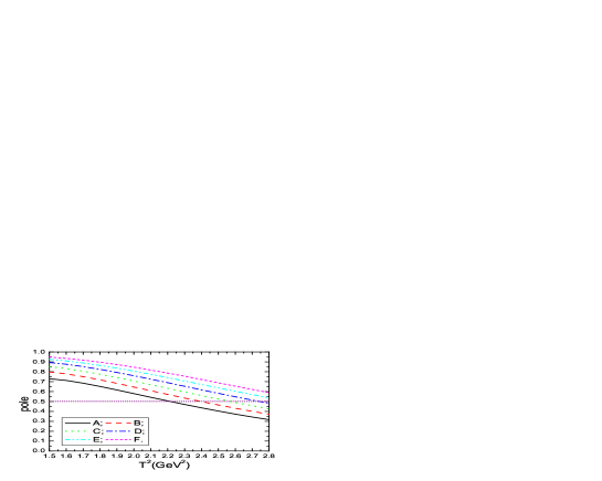
In Fig.3, the contribution of the pole term is plotted with variations of the threshold parameter $s_{0}$ and Borel parameter $T^{2}$ at the energy scale $\mu=1.3\,\rm{GeV}$. From the figure, we can see that the value $\sqrt{s_{0}}\leq 4.1\,\rm{GeV}$ is too small to satisfy the pole dominance condition and result in reasonable Borel window.

Refer to caption
Figure 3: The pole contribution with variations of the Borel parameter $T^{2}$ and threshold parameter $s_{0}$, where the $A$, $B$, $C$, $D$, $E$, $F$ denote the threshold parameters $\sqrt{s_{0}}=4.0$, $4.1$, $4.2$, $4.3$, $4.4$, $4.5\,\rm{GeV}$, respectively.

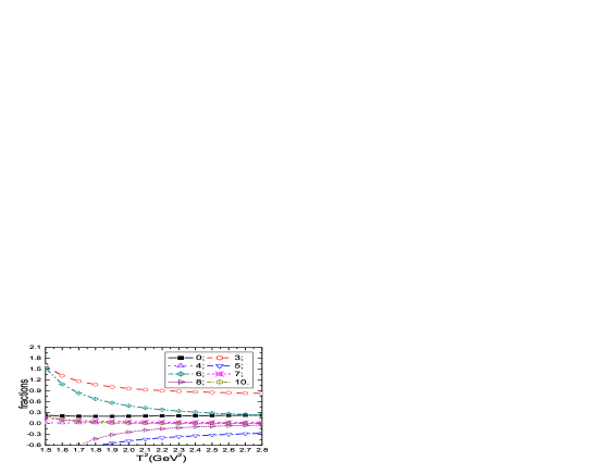
In Fig.4, the contributions of different terms in the operator product expansion are plotted with variations of the Borel parameter $T^{2}$ for the threshold parameter $\sqrt{s_{0}}=4.3\,\rm{GeV}$ at the energy scale $\mu=1.3\,\rm{GeV}$. From the figure, we can see that the $D_{0}$, $D_{3}$, $D_{5}$, $D_{6}$ and $D_{8}$, where the $D_{i}$ denote the contributions of the vacuum condensates of dimensions $D=i$, play an important role, while the $D_{4}$, $D_{7}$ and $D_{10}$ play a minor important role. At the value $T^{2}\leq 2.0\,\rm{GeV}$, the $D_{3}$, $D_{5}$, $D_{6}$ and $D_{8}$ decrease monotonously and quickly with increase of the $T^{2}$, which cannot lead to stable QCD sum rules. At the value $T^{2}=(2.2-2.6)\,\rm{GeV}^{2}$, $D_{3}\gg|D_{5}|\gg D_{6}\gg|D_{8}|$ and $D_{10}\ll 1\%$, the operator product expansion is well convergent, although $D_{0}\approx 20\%$. We approximate the continuum spectral density by ρQ​C​D​(s)β€‹Ξ˜β€‹(sβˆ’s0)subscriptπœŒπ‘„πΆπ·π‘ Ξ˜π‘ subscript𝑠0\rho_{QCD}(s)\Theta(s-s_{0}); the contributions of the quark condensate $\langle\bar{q}q\rangle$ and mixed condensate ⟨q¯​gs​σ​G​q⟩delimited-βŸ¨βŸ©Β―π‘žsubscriptπ‘”π‘ πœŽπΊπ‘ž\langle\bar{q}g_{s}\sigma Gq\rangle can be very large.

Refer to caption
Figure 4: The contributions of different terms in the operator product expansion with variations of the Borel parameter $T^{2}$, where the 0, 3, 4, 5, 6, 7, 8, 10 denote the dimensions of the vacuum condensates.

In this article, we take the Borel parameter $T^{2}=(2.2-2.6)\,\rm{GeV}^{2}$, the continuum threshold parameter $\sqrt{s_{0}}=(4.2-4.4)\,\rm{GeV}$ and the energy scale $\mu=1.3\,\rm{GeV}$, the pole dominance is well satisfied. The Borel parameter, continuum threshold parameter and the pole contribution are shown explicitly in Table 1. The two criteria (pole dominance and convergence of the operator product expansion) of the QCD sum rules are fully satisfied, furthermore, the relations in Eq.(33) and Eq.(35) are also satisfied.

$J^{PC}$ $T^{2}(\rm{GeV}^{2})$ $\sqrt{s_{0}}(\rm{GeV})$ pole $M_{Z}(\rm{GeV})$ $\lambda_{Z}$
$0^{++}$ $2.2-2.6$ $4.3\pm 0.1$ $(49-74)\%$ $3.82^{+0.08}_{-0.08}$ $1.79^{+0.29}_{-0.24}\times 10^{-2}\rm{GeV}^{5}$
Table 1: The Borel parameter, continuum threshold parameter, pole contribution, mass and pole residue of the scalar tetraquark state.
Refer to caption
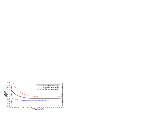
Figure 5: The mass with variations of the Borel parameter $T^{2}$.

Taking into account all uncertainties of the input parameters, finally we obtain the values of the mass and pole residue of the $S\bar{S}$ type scalar tetraquark state, which are shown explicitly in Figs.5-6 and Table 1.

The central value of the present prediction $M_{Z_{c}}=\left(3.82^{+0.08}_{-0.08}\right)\,\rm{GeV}$ for the $S\bar{S}$ type scalar tetraquark state is smaller than that of the $A\bar{A}$ type scalar tetraquark state $M_{J=0}=\left(3.85^{+0.15}_{-0.09}\right)\,\rm{GeV}$ obtained in Ref.[14]. The predictions based on the QCD sum rules are consistent with the values $M_{J=0}=3.852\,\rm{GeV}$ and $3.812\,\rm{GeV}$ for the $A\bar{A}$ and $S\bar{S}$ type scalar tetraquark states $cq\bar{c}\bar{q}$ respectively from the quasipotential approach [8].

Now we take the mass $M_{Z_{c}}$ and pole residue $\lambda_{Z_{c}}$ as basic input parameters to study the hadronic coupling constants $G_{Z_{c}\eta_{c}\pi}$ and $G_{Z_{c}DD}$, and take the same threshold parameter and Borel parameter as in the QCD sum rule for the mass and pole residue. In calculations, we choose the unknown parameters as $C_{Z_{c}\eta_{c}\pi}=0.0009\,\rm{GeV}^{6}$ and $C_{Z_{c}DD}=0.0004\,\rm{GeV}^{6}$ to obtain stable QCD sum rules with variations of the Borel parameter $T^{2}$ at the Borel windows $T^{2}=(2.2-2.6)\,\rm{GeV}^{2}$; the left side and right side of the QCD sum rules coincide. In fact, it is not necessary to choose the same Borel parameters both in the two-point and three-point QCD sum rules. If we take larger Borel parameter, say $T^{2}=(2.5-3.0)\,\rm{GeV}^{2}$ instead of $T^{2}=(2.2-2.6)\,\rm{GeV}^{2}$, we should alter the unknown parameters $C_{Z_{c}\eta_{c}\pi}$ and $C_{Z_{c}DD}$ slightly, then obtain stable QCD sum rules, the resulting values of the hadronic coupling constants change slightly.

Refer to caption
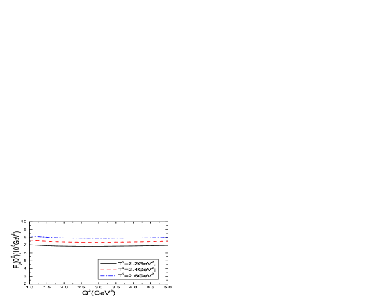
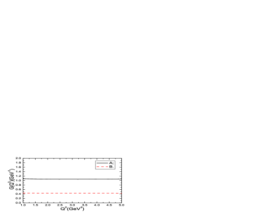
Figure 6: The pole residue with variations of the Borel parameter $T^{2}$.
Refer to caption
Figure 7: The central values of the $F_{2}(Q^{2})$ with variations of the $Q^{2}$.
Refer to caption
Figure 8: The central values of the hadronic coupling constants with variations of the $Q^{2}$, where the $A$ and $B$ denote the $G_{Z_{c}DD}(Q^{2})$ and $G_{Z_{c}\eta_{c}\pi}(Q^{2})$, respectively.

Based on Eqs.(30-31), we can study the $Q^{2}$ dependence of the right side of the QCD sum rules,

$\displaystyle F_{1}(Q^{2})$ $\displaystyle\propto$ $\displaystyle\frac{Q^{2}+M_{\pi}^{2}}{Q^{2}}\approx 1\,,$ (38)

at the region of large (or intermediate) $Q^{2}$ due to the tiny mass of the $\pi$, while the $F_{2}(Q^{2})$ has no such simple $Q^{2}$ dependence due to the heavy quark mass $m_{c}$ and heavy meson mass $M_{D}$. In the limit $Q^{2}\to\infty$,

$\displaystyle F_{2}(Q^{2})$ $\displaystyle=$ βˆ’mcβ€‹βŸ¨q¯​gs​σ​G​q⟩64​π2β€‹βˆ«01𝑑x​{1+x1βˆ’x​exp⁑(βˆ’mc2(1βˆ’x)​T2)+2βˆ’xx​exp⁑(βˆ’mc2T2)},subscriptπ‘šπ‘delimited-βŸ¨βŸ©Β―π‘žsubscriptπ‘”π‘ πœŽπΊπ‘ž64superscriptπœ‹2superscriptsubscript01differential-dπ‘₯1π‘₯1π‘₯superscriptsubscriptπ‘šπ‘21π‘₯superscript𝑇22π‘₯π‘₯superscriptsubscriptπ‘šπ‘2superscript𝑇2\displaystyle-\frac{m_{c}\langle\bar{q}g_{s}\sigma Gq\rangle}{64\pi^{2}}\int_{0}^{1}dx\left\{\frac{1+x}{1-x}\exp\left(-\frac{m_{c}^{2}}{(1-x)T^{2}}\right)+\frac{2-x}{x}\exp\left(-\frac{m_{c}^{2}}{T^{2}}\right)\right\}\,, (39)

which is independence on $Q^{2}$. In Fig.7, we plot the central values of the $F_{2}(Q^{2})$ with variations of the $Q^{2}$ at the range $Q^{2}=(1-5)\,\rm{GeV}^{2}$ for the Borel parameters $T^{2}=2.2\,\rm{GeV}^{2}$, $2.4\,\rm{GeV}^{2}$ and $2.6\,\rm{GeV}^{2}$, respectively. From the figure, we can see that the $Q^{2}$ dependence of the $F_{2}(Q^{2})$ is rather mild and can be neglected approximately. The left sides of the QCD sum rules in Eqs.(30-31) have no explicit $Q^{2}$ dependence, the $Q^{2}$ dependence is embodied in the right sides of the QCD sum rules ($F_{1}(Q^{2})$ and $F_{2}(Q^{2})$), so the hadronic coupling constants $G_{Z_{c}\eta_{c}\pi}$ and $G_{Z_{c}DD}$ are independent on the $Q^{2}$ in the limit $Q^{2}\rightarrow\infty$, the conclusion survives even for much smaller $Q^{2}$, say $Q^{2}=(1-5)\,\rm{GeV}^{2}$ according to Eq.(38) and Fig.7. The central values of the $G_{Z_{c}\eta_{c}\pi}(Q^{2})$ and $G_{Z_{c}DD}(Q^{2})$ can be fitted to the following constant forms,

$\displaystyle G_{Z_{c}\eta_{c}\pi}(Q^{2})$ $\displaystyle=$ $\displaystyle 0.43\,\rm{GeV}^{-1}\,,$
$\displaystyle G_{Z_{c}DD}(Q^{2})$ $\displaystyle=$ $\displaystyle 1.06\,\rm{GeV}^{-1}\,,$ (40)

at the region $Q^{2}=(1-5)\,\rm{GeV}^{2}$; the uncertainties of the $G_{Z_{c}\eta_{c}\pi}$ and $G_{Z_{c}DD}$ are about $25\%$ and $18\%$, respectively. We plot the central values of the hadronic coupling constants $G_{Z_{c}DD}(Q^{2})$ and $G_{Z_{c}\eta_{c}\pi}(Q^{2})$ with variations of the $Q^{2}$ at the region $Q^{2}=(1-5)\,\rm{GeV}^{2}$ for the Borel parameter $T^{2}=2.4\,\rm{GeV}^{2}$ in Fig.8. From the figure, we can see that the fitted functions in Eq.(40) are satisfactory. We extend the coupling constants to the physical regions without difficulty, and calculate the partial decay widths,

$\displaystyle\Gamma_{Z_{c}\to\eta_{c}\pi}$ $\displaystyle=$ $\displaystyle\frac{G_{Z_{c}\eta_{c}\pi}^{2}(M_{Z_{c}}^{2}-M_{\eta_{c}}^{2}-M_{\pi}^{2})^{2}\,p_{\eta_{c}\pi}}{32\pi M_{Z_{c}}^{2}}=(3.0\pm 1.5)\,\rm{MeV}\,,$
$\displaystyle\Gamma_{Z_{c}\to DD}$ $\displaystyle=$ $\displaystyle\frac{G_{Z_{c}DD}^{2}(M_{Z_{c}}^{2}-M_{D^{+}}^{2}-M_{D^{0}}^{2})^{2}\,p_{DD}}{32\pi M_{Z_{c}}^{2}}=(17.9\pm 6.4)\,\rm{MeV}\,,$ (41)

where

$\displaystyle p_{\eta_{c}\pi}$ $\displaystyle=$ $\displaystyle\frac{\sqrt{\left[M_{Z_{c}}^{2}-(M_{\eta_{c}}+M_{\pi})^{2}\right]\left[M_{Z_{c}}^{2}-(M_{\eta_{c}}-M_{\pi})^{2}\right]}}{2M_{Z_{c}}}\,,$
$\displaystyle p_{DD}$ $\displaystyle=$ $\displaystyle\frac{\sqrt{\left[M_{Z_{c}}^{2}-(M_{D^{+}}+M_{D^{0}})^{2}\right]\left[M_{Z_{c}}^{2}-(M_{D^{+}}-M_{D^{0}})^{2}\right]}}{2M_{Z_{c}}}\,.$ (42)

The total width $\Gamma_{Z_{c}}$ of the $Z_{c}(3820)$ can be approximated by $\Gamma_{Z_{c}\to\eta_{c}\pi}+\Gamma_{Z_{c}\to DD}$, the numerical value is about $(20.9\pm 6.6)\,\rm{MeV}$. The radiative decay widths can be estimated by assuming vector meson dominance, for example, $\Gamma_{Z_{c}^{\pm}\to\gamma\rho^{\pm}}\propto\alpha|\Gamma_{Z^{\pm}_{c}\to J/\psi^{*}\rho^{\pm}}|$ for the radiative decays $Z^{\pm}_{c}(3820)\to J/\psi^{*}\rho^{\pm}\to\gamma\rho^{\pm}$, the partial decay widths are of the order ${\cal{O}}(\rm{KeV})$ due to the factor $\alpha=\frac{e^{2}}{4\pi}=\frac{1}{137}$. The strong decays $Z^{\pm}_{c}(3820)\to J/\psi\rho^{\pm}$ are kinematically forbidden, the values of the $\Gamma_{Z^{\pm}_{c}\to J/\psi^{*}\rho^{\pm}}$ are complex, so we take $|\Gamma_{Z^{\pm}_{c}\to J/\psi^{*}\rho^{\pm}}|$. The contributions of the radiative decays to the total width $\Gamma_{Z_{c}}$ are small and can be neglected.

4 Conclusion

In this article, we calculate the contributions of the vacuum condensates up to dimension-10 in the operator product expansion, study the $S\bar{S}$ type scalar tetraquark state $cq\bar{c}\bar{q}$ in details with the QCD sum rules. In calculations, we search for the optimal Borel parameter and threshold parameter to satisfy the energy scale formula $M^{2}_{Z}=(2{\mathbb{M}}_{c})^{2}+\mu^{2}$ and the experiential threshold formula $\sqrt{s_{0}}=M_{Z}+(0.4-0.6)\,\rm{GeV}$, where the $\mu$ is the energy scale of the QCD spectral density, and obtain the values $M_{Z_{c}}=\left(3.82^{+0.08}_{-0.08}\right)\,\rm{GeV}$ and $\lambda_{Z_{c}}=\left(1.79^{+0.29}_{-0.24}\right)\times 10^{-2}\rm{GeV}^{5}$. The central value of the mass of the $S\bar{S}$ type scalar tetraquark state is smaller than that of the $A\bar{A}$ type scalar tetraquark state, the $S\bar{S}$ type scalar tetraquark state $cq\bar{c}\bar{q}$ maybe the lowest hidden charmed tetraquark state. Furthermore, we calculate the hadronic coupling constants $G_{Z_{c}\eta_{c}\pi}$ and $G_{Z_{c}DD}$ with the three-point QCD sum rules by taking into account the color-connected diagrams, then study the strong decays $Z_{c}\to\eta_{c}\pi\,,\,DD$, and observe that the total width $\Gamma_{Z_{c}}\approx 21\,\rm{MeV}$. The present predictions can be confronted with the experimental data in the futures at the BESIII, LHCb and Belle-II.

Acknowledgements

This work is supported by National Natural Science Foundation, Grant Numbers 11375063, and Natural Science Foundation of Hebei province, Grant Number A2014502017.

References

  • [1] M. Huang, Int. J. Mod. Phys. E14 (2005) 675.
  • [2] A. De Rujula, H. Georgi and S. L. Glashow, Phys. Rev. D12 (1975) 147.
  • [3] T. DeGrand, R. L. Jaffe, K. Johnson and J. E. Kiskis, Phys. Rev. D12 (1975) 2060.
  • [4] Z. G. Wang, Eur. Phys. J. C71 (2011) 1524.
  • [5] R. T. Kleiv, T. G. Steele and A. Zhang, Phys. Rev. D87 (2013) 125018.
  • [6] Z. G. Wang, Phys. Rev. D79 (2009) 094027.
  • [7] Z. G. Wang, Eur. Phys. J. C67 (2010) 411.
  • [8] D. Ebert, R. N. Faustov and V. O. Galkin, Eur. Phys. J. C58 (2008) 399.
  • [9] L. Maiani, F. Piccinini, A. D. Polosa and V. Riquer, Phys. Rev. D71 (2005) 014028.
  • [10] L. Maiani, F. Piccinini, A. D. Polosa and V. Riquer, Phys. Rev. D89 (2014) 114010.
  • [11] Z. G. Wang and T. Huang, Phys. Rev. D89 (2014) 054019.
  • [12] Z. G. Wang, Eur. Phys. J. C74 (2014) 2874.
  • [13] Z. G. Wang and T. Huang, Nucl. Phys. A930 (2014) 63.
  • [14] Z. G. Wang, arXiv:1312.1537.
  • [15] Z. G. Wang and T. Huang, Eur. Phys. J. C74 (2014) 2891.
  • [16] Z. G. Wang, Eur. Phys. J. C74 (2014) 2963.
  • [17] M. A. Shifman, A. I. Vainshtein and V. I. Zakharov, Nucl. Phys. B147 (1979) 385.
  • [18] M. A. Shifman, A. I. Vainshtein and V. I. Zakharov, Nucl. Phys. B147 (1979) 448.
  • [19] L. J. Reinders, H. Rubinstein and S. Yazaki, Phys. Rept. 127 (1985) 1.
  • [20] F. S. Navarra and M. Nielsen, Phys. Lett. B639 (2006) 272.
  • [21] J. M. Dias, F. S. Navarra, M. Nielsen and C. M. Zanetti, Phys. Rev. D88 (2013) 016004.
  • [22] P. Colangelo and A. Khodjamirian, hep-ph/0010175.
  • [23] B. L. Ioffe, Prog. Part. Nucl. Phys. 56 (2006) 232.
  • [24] J. Beringer et al, Phys. Rev. D86 (2012) 010001.
  • [25] Z. G. Wang, JHEP 1310 (2013) 208.
  • [26] V. A. Novikov, L. B. Okun, M. A. Shifman, A. I. Vainshtein, M. B. Voloshin and V. I. Zakharov, Phys. Rept. 41 (1978) 1.
  • [27] M. Nielsen and F. S. Navarra, Mod. Phys. Lett. A29 (2014) 1430005.
  • [28] Z. G. Wang, arXiv:1405.3581.