Eccentric first post-Newtonian waveforms for compact binaries in frequency domain with Hansen coefficients

Abstract

The inspiral and merger of supermassive black hole binary systems with high orbital eccentricity are among the promising sources of the advanced gravitational wave observatories. In this paper we derive analytic ready-to-use first post-Newtonian eccentric waveform in Fourier domain with the use of Hansen coefficients. Introducing generic perturbations of celestial mechanics we have generalized the Hansen expansion to the first post-Newtonian order which are then used to express the waveforms. Taking into account the high eccentricity of the orbit leads to the appearance of secular terms in the waveform which are eliminated with the introduction of a phase shift. The waveforms have a systematic structure and as our main result these are expressed in a tabular form.

I Introduction

Compact binaries (i. e. black holes, neutron stars and white dwarfs) with non-vanishing eccentricity are promising sources of gravitational waves. Depending on their parameters these sources emit radiation within the sensitivity band of the forthcoming gravitational wave detectors advanced LIGO and Virgo. Due to their increased sensitivity the source signals will be visible by these detectors for a longer time period with the requirement of an accurate description of both the orbital evolution and the emitted GWs of these systems. detectability The measured signal output of the detectors is cross correlated with theoretical waveform templates in matched filtering. The presence of orbital eccentricity changes significantly the properties of the waveforms resulting in the decrease of their detectability with the use of circular templates.In spite of the general circularization of binary orbits due to GW emission binaries interacting with their environment can retain non-negligible eccentricity at the end of their evolution. For example, there are indications that binaries in dense galactic nuclei LearyKocsis ; KocsisLevin , embedded in a gaseous disk Cuadra ; Sesana can remain eccentric  until the end of their inspiral. Moreover, the interaction of supermassive black hole binaries with star populations Preto ; Lockman and the Kozai mechanism and relativistic orbital resonances in hierarchial triples Wen ; Hoffman ; Seto ; NaozKocsis can also increase orbital eccentricity.

The first analytic eccentric waveform for the unperturbed motion was given by Whalquist . The time-dependent waveform is computed with the help of Fourier-Bessel method in Ref. Moreno and the waveform in Fourier space for arbitrary eccentricity was given in Ref mikoczi .

Recently, within the post-Newtonian (PN) treatment of compact binary evolution the theoretical computations are reaching the level of 4PN. The first post-Newtonian eccentric waveform for bound orbits is computed by Wagoner and Will Wagoner in 1976. The description of the Kepler motion with the 1PN correction is given by Damour and Deruelle in Ref DD which requires three eccentricities (radial, time and angular eccentricity). With the help of this Damour-Deruelle parameterization the eccentric waveform and evolution of the semimajor axis and the radial eccentricity due to radiation reaction is computed by Junker and Schäfer in Ref Junker . The waveform in Fourier domain up to 1PN and 2PN orders are given in Refs. Tessmer ,Tessmer2 .

Our work focuses on ready-to-use eccentric 1PN waveforms in frequency domain. In our description we use the generalized true anomaly parameterization which has the advantage that the solution of the equations of motion can be expressed with only two eccentricities. As a consequence, the gravitational waveforms have a simple structure. Secular terms appearing in the waveforms are eliminated by the use of the Poincaré-Lindstedt method and the introduction of the drift true anomaly parameter. We give both the time-dependent and frequency domain waveforms using the Hansen expansion and the stationary phase approximation (SPA). Moreover, we compute the evolution of the semimajor axis and radial eccentricity up to 1PN accuracy.

The paper is organized as follows. After a short summary of the Damour-Deruelle parameterization in Sec. II we introduce the generalized true anomaly parameterization in Sec. III and the 1PN waveform in Sec. IV. Sec. V. contains the extension of the Hansen coefficients to 1PN order. Fourier domain SPA waveforms are given in Sec VI. The radiation reaction problem and the evolution of the time and phase functions to 1PN order are given in Sec VII. Some of the technical details, i.e. tensor spherical harmonics, orbital parameters to 1PN order, Hansen coefficients and waveform expressions are presented in the Appendices.

II Damour-Deruelle parameterization

In the following, we summarize the first post-Newtonian parameterization of the orbital motion introduced by Damour and Deruelle DD for the description of compact binaries. The Lagrangian of the system contains the Newtonian and 1PN corrections,

$$\mathcal{L} \mathcal{=} \frac{\mu}{2}\mathbf{v}^{2}+\frac{Gm\mu}{r}$$ (1)

$$+\frac{1}{8c^{2}}\left(1-3\eta\right)\mu\mathbf{v}^{4}+\!\frac{Gm\mu}{2rc^{2}}\!\left[\!\left(3\!+\!\eta\right)\mathbf{v}^{2}\!+\!\eta\dot{r}^{2}\!-\!\frac{Gm}{r}\!\right]\mathbf{\ ,}$$

where $r$ is the relative distance, $\mathbf{v}$ is the relative velocity vector, $m=m_{1}+m_{2}$ is the total mass, $\mu=m_{1}m_{2}/m$ is the reduced mass and $\eta=\mu/m$ is the symmetric mass ratio. The overdot denotes the derivative with respect to time $t$. The radial and angular motion can be separated to the linear order, so the Euler-Lagrange equation are

$$\left(\frac{dr}{dt}\right)^{2} =A+\frac{2B}{r}+\frac{C}{r^{2}}+\frac{D}{r^{3}}\mathbf{\ ,}$$ (2)

$$\frac{d\theta}{dt} =\frac{H}{r^{2}}+\frac{I}{r^{3}}\mathbf{\ ,}$$ (3)

where $\theta$ is the azimuthal angle in the orbital plane and the constants $A,B,C,D,H,I$ depend on the conserved quantities such as energy and the orbital angular momentum of the perturbed motion, see Appendix B. The constants $A,B,C,H$ contain Newtonian and 1PN terms while $D$ and $I$ are purely 1PN corrections. The equations of motion, Eqs. (2,3) can be solved by the eccentric anomaly quasi-parameterization $u$, that is

$$r=a_{r}(1-e_{r}\cos u)\mathbf{\ ,}$$ (4)

where the orbital parameters are the semimajor axis $a_{r}$ and the radial eccentricity $e_{r}$. These orbital parameters are characterized by the turning points ($r_{\max}$ and $r_{\min}$ in KMG ,KJ ) of the radial motion. The Kepler equation and angular evolution can be given as

$$n(t-t_{0}) = u-e_{t}\sin u\equiv\mathcal{M}\mathbf{\ ,}$$ (5)

$$\theta-\theta_{0} = (1+k)v_{\theta}\mathbf{\ ,}$$ (6)

$$v_{\theta} = 2\arctan\sqrt{\frac{1+e_{\theta}}{1-e_{\theta}}}\tan\frac{u}{2}\mathbf{,}$$ (7)

in terms of the orbital elements of the 1PN orbital dynamics such as the mean motion $n$, the time eccentricity $e_{t}$, the angle eccentricity $e_{\theta}$, and the pericenter drift $k$ (which is in relationship with the pericenter precession $\left\langle\dot{\gamma}\right\rangle$ averaged over one radial period, see mikoczi ). In the above equations $t_{0}$ and $\theta_{0}$ are integration constants and in our calculations we set $\theta_{0}=t_{0}=0$. The Damour-Deruelle parameterization contains three eccentricities, which are different in 1PN order only. In Newtonian order only the Kepler equation and one eccentricity remain.

We note that the Kepler equation remains the same with the inclusion of the spin-orbit interaction (see ref. Wex ) but it contains higher order contributions such as the spin-spin, quadrupole-monopole and magnetic dipole-dipole interactions KMG or the second post-Newtonian corrections SW . For this reason we use an other parameterization which has only two eccentricities and the evolution of the azimuthal angle $\theta$ is similarly simple as Eq. (6).

III Generalized true anomaly parameterization

We introduce the generalized true anomaly parameterization $\phi$ (denoted by $\chi$ in param ,KMG ) as

$$r=\frac{a_{r}(1-e_{r}^{2})}{1+e_{r}\cos\phi}\mathbf{\ .}$$ (8)

This parameterization has a similar form than the Keplerian parameterization, where the orbital parameters $a_{r}$ and $e_{r}$ include only the leading order Newtonian terms. Eqs. (8) and (4) lead to the relation $\phi=v_{r}=2\arctan\left[\left(1+e_{r}\right)^{1/2}\left(1-e_{r}\right)^{-1/2}\tan\left(u/2\right)\right]$, cf. Eq. (7).

The time evolution of the generalized true anomaly up to 1PN order can be expressed as

$$\dot{\phi}=\frac{na_{r}^{2}(1-e_{r}^{2})^{3/2}}{r^{2}(1-e_{t}e_{r}+(e_{r}-e_{t})\cos\phi)}\mathbf{\ .}$$ (9)

The integration of Eq. (3) with the help of (9) leads to the relation

$$\theta-\theta_{0}=\left(1+\kappa_{1}\right)\phi+\kappa_{2}\sin\phi\mathbf{,}$$ (10)

where we have introduced the 1PN order quantities $\kappa_{1}=3Gm/[a_{r}(1-e_{r}^{2})c^{2}]$ and $\kappa_{2}=G\mu e_{r}/[2a_{r}(1-e_{r}^{2})c^{2}]$. In this parameterization only radial and time eccentricities ($e_{r}$, $e_{t}$) appear while angle eccentricity does not. The relationship between $\phi$ and $v_{\theta}$ is given by Eqs. (6) and (10) up to 1PN order as

$$\phi=v_{\theta}-\frac{G\mu e_{r}}{2a_{r}(1-e_{r}^{2})c^{2}}\sin v_{\theta}.$$ (11)

In the following we will compute the full eccentric 1PN waveform with the use of the generalized true anomaly parameterization $\phi$ without the appearance of secular terms in the expressions and give the time-domain waveforms using the generalized Hansen expansion. Our aim is to express the full analytic eccentric frequency-domain waveform up to 1PN order.

IV Waveform

The first explicit description of the 1PN waveform for binaries was given by Wagoner and Will in 1976 Wagoner . We rewrite their expressions with help of Ref. Thorne and, as a result, the radiation field up to 1PN order has the following form

$$h_{ij}^{TT} = \varepsilon^{4}\frac{G}{D_{L}}\Biggl{\{}\sum_{m=-2}^{2}\overset{(2)}{I}_{2m}T_{ij}^{E2,2m}+\epsilon\Biggl{[}\sum_{m=-2}^{2}{\overset{(2)}{S}}_{2m}\,T_{ij}^{B2,2m}$$ (13)

$$+\sum_{m=-3}^{3}\overset{(3)}{I}_{3m}T_{ij}^{E2,3m}\Biggr{]}\Biggr{\}}\,.$$

Here $D_{L}$ is the luminosity distance, $\varepsilon=Gm/c^{2}r$ is the post-Newtonian parameter, $T_{ij}^{E2,km}$and $T_{ij}^{B2,km}$ are the tensorial electric and magnetic scalar harmonics which are given by Eq. (2.30d) in Thorne . The quantities $\overset{(k)}{I}_{km},$ ${\overset{(k)}{S}}_{km}$ are the $k$th time derivatives of the mass and current multipole moments. The explicit form of these multipoles was given by Junker and Schäfer in 1PN order with eccentric anomaly $u$ in refs. Junker and Tessmer . Later, the authors of Tessmer2 have computed the explicit time-dependent multipoles $\overset{(k)}{I}_{km}$ and ${\overset{(k)}{S}}_{km}$ up to 2PN. Their waveforms contain no secular terms because the authors are not using Eq. (6) but the exponents containing $\theta$ have been expressed as series in $\overset{(k)}{I}_{km},$ ${\overset{(k)}{S}}_{km}$.

It is well-known that some secular terms will appear in the eccentric waveforms if one expands the harmonic functions of the angle $\theta$ in terms of the generalized true anomaly parameterization. These secular terms have to be eliminated in the waveforms which requires the introduction of the drift true anomaly $\phi^{\prime}=\left(1+\kappa_{1}\right)\phi$. Then the harmonic functions of $\theta$ can be described in a perturbative sense (see Soffel ) as

$$\cos\theta \approx \cos\phi^{\prime}-\kappa_{2}\sin\phi\sin\phi^{\prime},$$ (14)

$$\sin\theta \approx \sin\phi^{\prime}+\kappa_{2}\sin\phi\cos\phi^{\prime},$$ (15)

which relations will be used to eliminate secular terms in the eccentric waveforms.

The waveform up to 1PN order for the polarization states are

$$h_{+,\times}(\phi)=h_{+,\times}^{N}(\phi)+h_{+,\times}^{H}(\phi)+h_{+,\times}^{PN}(\phi)\mathbf{.}$$ (16)

The $h_{+,\times}^{N}(\phi)$ is the Newtonian, $h_{+,\times}^{H}(\phi)$ is the half order PN and $h_{+,\times}^{PN}(\phi)$ is the 1PN waveform (see Appendix D and E). Our 1PN waveform has the well-known structure with the generalized true anomaly $\phi$ and drift anomaly $\phi^{\prime}$, as

$$h_{+,\times}^{PN}(\phi) = \sum_{m=0}^{4}\Biggl{[}\left(c_{m(c4)}^{+,\times}\cos m\phi+s_{m(c4)}^{+,\times}\sin m\phi\right)\cos 4\phi^{\prime}$$ (17)

$$+\left(c_{m(s4)}^{+,\times}\cos m\phi+s_{m(s4)}^{+,\times}\sin m\phi\right)\sin 4\phi^{\prime}$$

$$+\left(c_{m(c2)}^{+,\times}\cos m\phi+s_{m(c2)}^{+,\times}\sin m\phi\right)\cos 2\phi^{\prime}$$

$$+\left(c_{m(s2)}^{+,\times}\cos m\phi+s_{m(s2)}^{+,\times}\sin m\phi\right)\sin 2\phi^{\prime}$$

$$+\left(c_{m}^{+,\times}\cos m\phi+s_{m}^{+,\times}\sin m\phi\right)\Biggr{]}\mathbf{,}$$

where the coefficients $c_{m(c4)}^{+,\times}$, $s_{m(c4)}^{+,\times}$,$c_{m(c2)}^{+,\times}$, $s_{m(c4)}^{+,\times}$, $c_{m}^{+,\times}$ and $s_{m}^{+,\times}$ depend on  the radial eccentricity $e_{r}$, the mass parameters $m$, $\mu$, $\eta$ and the two polar angles $\Theta$ and $\Phi$ of the line of sight (see Appendix E). We introduce the quantities

$$\phi_{m}^{\pm 4} = m\phi\pm 4\phi^{\prime}=m_{4\pm}\phi\mathbf{\ ,}$$ (18)

$$\phi_{m}^{\pm 2} = m\phi\pm 2\phi^{\prime}=m_{2\pm}\phi\mathbf{\ ,}$$ (19)

$$\phi_{m} = m\phi\mathbf{\ ,}$$ (20)

with the real numbers $m_{4\pm}=m\pm 4\left(1+\kappa_{1}\right)$, $m_{2\pm}=m\pm 2\left(1+\kappa_{1}\right)$ and coefficients

$$C_{m,+,\times}^{\pm 4} = \frac{c_{m(c4)}^{+,\times}\mp s_{m(s4)}^{+,\times}}{2}\mathbf{\ ,}\mathcal{\qquad}S_{m,+,\times}^{\pm 4}=\frac{s_{m(c4)}^{+,\times}\pm c_{m(s4)}^{+,\times}}{2}\mathbf{\ ,}$$ (21)

$$C_{m,+,\times}^{\pm 2} = \frac{c_{m(c2)}^{+,\times}\mp s_{m(s2)}^{+,\times}}{2}\mathbf{\ ,}\mathcal{\qquad}S_{m,+,\times}^{\pm 2}=\frac{c_{m(c2)}^{+,\times}\pm s_{m(s2)}^{+,\times}}{2}\mathbf{\ .}$$ (22)

We can use the Hansen expansion for the generalized true anomalies as

$$\cos\lambda\phi=\sum_{k=0}^{\infty}C_{k}^{\lambda}\cos k\mathcal{M},\mathcal{\qquad}\sin\lambda\phi=\sum_{k=0}^{\infty}S_{k}^{\lambda}\sin k\mathcal{M}\mathbf{\ ,}$$ (23)

with $C_{0}^{\lambda}=X_{0}^{0,\lambda}$, $C_{k}^{\lambda}=X_{k}^{0,\lambda}+X_{-k}^{0,\lambda}$ and $S_{k}^{\lambda}=X_{k}^{0,\lambda}-X_{-k}^{0,\lambda}$ where $X_{k}^{n,\lambda}$ are the generalized Hansen coefficients for the real number $\lambda$ (since $\kappa_{1}$ is not integer) up to 1PN order. We note that in the Keplerian case (where $\lambda$ is integer and $e=e_{r}=e_{t}=e_{\theta}$) $\cos\lambda\phi$ and $\sin\lambda\phi$ can be extended by trigonometric functions of $\cos\phi$   and $\sin\phi$. Using the Fourier coefficients containing Bessel-functions (see e.g. Brumberg )

$$\cos\phi = -e+\frac{2(1-e^{2})}{e}\sum_{k=1}^{\infty}J_{k}(ke)\cos k\mathcal{M},$$ (24)

$$\sin\phi = 2\sqrt{1-e^{2}}\sum_{k=1}^{\infty}\frac{J_{k}^{\prime}(ke)}{k}\sin k\mathcal{M},$$ (25)

where $\prime$ denotes the derivative with respect to the eccentricity $e$. This ’classical’ extension leads to an increasing order of sums for the increasing value of $\lambda$. Note that Eqs. (24) and (25) are not valid for the 1PN motion. Therefore we extend Hansen coefficients up to 1PN order in the next chapter.

V Generalization of Hansen coefficients

The Hansen coefficients are well-known already since the 19th century in celestial mechanics (see Appendix C). In our description of the time-dependent waveforms there appear Hansen coefficients therefore it is important to extend the Hansen expansion up to 1PN order. The $X_{k}^{n,m}$ Hansen coefficients appear in next series

$$\left(\frac{r}{a}\right)^{n}\exp(im\phi)=\overset{\infty}{\underset{k=-\infty}{\sum}}X_{k}^{n,m}\exp(ik\mathcal{M}).$$ (26)

The definition of Hansen coefficients are

$$X_{k}^{n,m}=\frac{1}{2\pi}\underset{-\pi}{\overset{\pi}{\int}}\left(\frac{r}{a}\right)^{n}\exp(imv-ik\mathcal{M})d\mathcal{M}.$$ (27)

In the waveform there appear the harmonic functions of $m\phi$ where$\ m$ is not an integer parameter. So we have to generalize the formula of the Keplerian Hansen coefficients Jarnagin ,

$$X_{k}^{n,m} = (1+\beta^{2})^{-n-1}\overset{\infty}{\underset{s=0}{\sum}}\overset{\infty}{\underset{t=0}{\sum}}\binom{n-m+1}{s}$$ (28)

$$\times\binom{n+m+1}{t}\left(-\beta\right)^{s+t}I_{k-m-s+t}(ke),$$

where $p=k-m-s+t$ is a index notation and $I_{p}(z)$ is the contour integral

$$I_{p}(z)=\frac{1}{2\pi i}\oint u^{-1-p}\exp\frac{z\left(u-u^{-1}\right)}{2}du.$$ (29)

It is evident if $p$ is an integer (i.e. $m$ is integer) then $I_{p}(z)=J_{p}(z)$ where $J_{p}(z)$ is the Bessel function (e.g. for the Newtonian waveform see mikoczi ). If $p$ is not an integer then $I_{p}(z)=J_{p}(z)+g_{p}(z)$, where $g_{p}(z)$ is the correction integral (WW )

$$g_{p}(z)=-\frac{\sin p\pi}{\pi}\underset{0}{\overset{\infty}{\int}}\exp(-pu-z\sinh u)du$$ (30)

for $R(z)>0$.

Due to the different eccentricities we have to generalize Hansen coefficient in a different way for case of 1PN order. The mean anomaly (see Eq. (87) in Appendix C) is

$$\frac{d\mathcal{M}}{du}=1-e_{t}\cos u.$$ (31)

We have introduced the complex quantity $y=\exp iu$, then

$$\frac{r}{a} = \left(1+\beta_{r}^{2}\right)^{-1}(1-\beta_{r}y)(1-\beta_{r}y^{-1}),$$ (32)

$$\frac{d\mathcal{M}}{du} = 1-\frac{e_{t}}{2}\left(y+y^{-1}\right),$$ (33)

where $\beta_{r}=\beta(e_{r})$ (see Appendix C, $\beta=(1-\sqrt{1-e^{2}})/e$ is the parameter in celestial mechanics). Then the integrand is

$$\left(X_{k}^{n,m}\right)_{PN} = \frac{\left(1+\beta_{r}^{2}\right)^{-n}}{2\pi}\underset{-\pi}{\overset{\pi}{\int}}y^{m-k}(1-\beta_{r}y^{-1})^{n+m}(1-\beta_{r}y)^{n-m}$$ (34)

$$\times\left(1-\frac{e_{t}\left(y+y^{-1}\right)}{2}\right)\exp\frac{ke_{t}\left(y-y^{-1}\right)}{2}du$$

which can be extended in a form of an infinite series of the sum. Then the generalized Hansen coefficients for 1PN order are

$$\left(X_{k}^{n,m}\right)_{PN} = (1+\beta_{r}^{2})^{-n}\overset{\infty}{\underset{s=0}{\sum}}\overset{\infty}{\underset{t=0}{\sum}}\binom{n-m}{s}\binom{n+m}{t}\left(-\beta_{r}\right)^{s+t}$$ (35)

$$\times\left[I_{p}(ke_{t})-\frac{e_{t}}{2}\left(I_{p-1}(ke_{t})+I_{p+1}(ke_{t})\right)\right].$$

If we use a new index notation $j=t-s$ then generalized Hansen coefficients for 1PN are

$$\left(X_{k}^{n,m}\right)_{PN} = (1+\beta_{r}^{2})^{-n}\overset{s_{1}}{\underset{s=0}{\sum}}\overset{j_{1}}{\underset{j=-s}{\sum}}\binom{n-m}{s}\binom{n+m}{s+j}\left(-\beta_{r}\right)^{j}$$ (36)

$$\times\left[I_{p}(ke_{t})-\frac{e_{t}}{2}\left(I_{p-1}(ke_{t})+I_{p+1}(ke_{t})\right)\right].$$

where $p=k-m+j$. We note that for an integer $m$ the square bracket in second line of Eq. (36) can be written as

$$[...]=\left(1-\frac{p}{k}\right)J_{p}(ke_{t})+\frac{\sin(p\pi)}{k\pi}.$$ (37)

Then the explicit time-dependent waveforms, Eq. (17), are

$$h_{+,\times}^{PN}(t)=\sum_{m=0}^{4}\sum_{k=0}^{\infty}\left(\mathcal{C}_{k}^{+,\times,m}\cos k\mathcal{M}+\mathcal{S}_{k}^{+,\times,m}\sin k\mathcal{M}\right)\mathbf{\ ,}$$ (38)

where

$$\mathcal{C}_{k}^{+,\times,m} = C_{m,+,\times}^{-4}C_{k}^{m_{4-}}+C_{m,+,\times}^{+4}C_{k}^{m_{4+}}+C_{m,+,\times}^{-2}C_{k}^{m_{2-}}$$ (39)

$$+C_{m,+,\times}^{+2}C_{k}^{m_{2+}}+c_{m}^{+,\times}C_{k}^{m},$$

$$\mathcal{S}_{k}^{+,\times,m} = S_{m,+,\times}^{-4}S_{k}^{m_{4-}}+S_{m,+,\times}^{+4}S_{k}^{m_{4+}}+S_{m,+,\times}^{-2}S_{k}^{m_{2-}}$$ (40)

$$+S_{m,+,\times}^{+2}S_{k}^{m_{2+}}+s_{m}^{+,\times}S_{k}^{m},$$

These waveform has significantly simpler structure than the corresponding expressions in Tessmer .

VI Waveform in Fourier space

The waveform in Fourier space can be described in the stationary phase approximation of the time-dependent waveform (see Eqs. (B2) and (B3) in the Appendix B of mikoczi ). Taking an arbitrary harmonic function $\mathcal{A}(t)\cos\Phi(t)$, where $\mathcal{A}(t)$, $\Phi(t)$ is the time-dependent amplitude and phase, respectively, and the conditions $\mathcal{\dot{A}}/\mathcal{A}\ll\dot{\Phi}$ and $\ddot{\Phi}\ll\dot{\Phi}^{2}$ are satisfied, then the Fourier transform of the function $\mathcal{A}(t)\cos\Phi(t)$ can be written as

$$\mathcal{F}\left[\mathcal{A}(t)\sin\Phi(t)\right] = \tfrac{\mathcal{A}\left[f(\mathcal{T})\right]}{2}\sqrt{\tfrac{2\pi}{\left|\ddot{\Psi}\left[f(\mathcal{T})\right]\right|}}e^{i\left(\Psi\left[f(\mathcal{T})\right]+\frac{\pi}{4}\right)}\ ,$$ (41)

$$\mathcal{F}\left[\mathcal{A}(t)\cos\Phi(t)\right] = \tfrac{\mathcal{A}\left[f(\mathcal{T})\right]}{2}\sqrt{\tfrac{2\pi}{\left|\ddot{\Psi}\left[f(\mathcal{T})\right]\right|}}e^{i\left(\Psi\left[f(\mathcal{T})\right]-\frac{\pi}{4}\right)}\ ,$$ (42)

where $\Psi\left[f(\mathcal{T})\right]=2\pi f(\mathcal{T})t\left[\nu(\mathcal{T})\right]-\Phi\left[\nu(\mathcal{T})\right]$ is the phasing function, $\mathcal{T}$ is the saddle point and the functions $t\left[\nu(\mathcal{T})\right]$ and $\Phi\left[\nu(\mathcal{T})\right]$ appearing in the above expressions can be obtained from the leading order equations for gravitational radiation by Appell functions (see the Appendix in mikoczi ). It is necessary to add, that here the phase and frequency ($\Psi_{n}$ and $\Psi_{n\pm}$) are not splitting into triplet due to pericenter precession (it was a consequence of the appearance of $\dot{\gamma}$, i.e. heuristic precession in mikoczi ), because it is contained directly the 1PN equations of motion (see the orbital parameter $k$). Therefore the 1PN waveform depends on the single phase and frequency $\Psi_{n}$. Accordingly, the waveform, Eq. (38), in the Fourier space becomes

$$h_{+}^{PN}(f) = \frac{1}{2}\sqrt{\tfrac{2\pi}{\left|\ddot{\Psi}\left[f(\mathcal{T})\right]\right|}}\sum_{m=0}^{4}\sum_{k=0}^{\infty}\Biggl{[}\mathcal{C}_{k}^{+,m}\left[f(\mathcal{T})\right]e^{i\left(\Psi\left[f(\mathcal{T})\right]-\frac{\pi}{4}\right)}$$ (43)

$$+\mathcal{S}_{k}^{+,m}\left[f(\mathcal{T})\right]e^{i\left(\Psi\left[f(\mathcal{T})\right]+\frac{\pi}{4}\right)}\Biggr{]},$$

$$h_{\times}^{PN}(f) = \frac{1}{2}\sqrt{\tfrac{2\pi}{\left|\ddot{\Psi}\left[f(\mathcal{T})\right]\right|}}\sum_{m=0}^{4}\sum_{k=0}^{\infty}\Biggl{[}\mathcal{C}_{k}^{\times,m}\left[f(\mathcal{T})\right]e^{i\left(\Psi\left[f(\mathcal{T})\right]-\frac{\pi}{4}\right)}$$ (44)

$$+\mathcal{S}_{k}^{\times,m}\left[f(\mathcal{T})\right]e^{i\left(\Psi\left[f(\mathcal{T})\right]+\frac{\pi}{4}\right)}\Biggr{]},$$

with the stationary phase condition $\left|\ddot{\Psi}\left[f(\mathcal{T})\right]\right|=2\pi n\dot{\nu}$ and the phasing function $\Psi\left[f(\mathcal{T})\right]=2\pi ft(\mathcal{T})-\Phi_{n}(\mathcal{T})$. The above form can be written as

$$h_{+}^{PN}(f) = \frac{\left(n\dot{\nu}\right)^{-1/2}}{2}\sum_{m,k=0}^{4,\infty}\Biggl{[}\mathcal{C}_{k}^{+,m}e^{i\Psi-}+\mathcal{S}_{k}^{+,m}e^{i\Psi+}\Biggr{]},$$ (45)

$$h_{\times}^{PN}(f) = \frac{\left(n\dot{\nu}\right)^{-1/2}}{2}\sum_{m,k=0}^{4,\infty}\Biggl{[}\mathcal{C}_{k}^{\times,m}e^{i\Psi-}+\mathcal{S}_{k}^{\times,m}e^{i\Psi+}\Biggr{]},$$ (46)

where the phasing functions are $\Psi_{\pm}=2\pi ft(\mathcal{T})-\Phi_{n}(\mathcal{T})\pm\pi/4$.

Afterwards we shall compute the phase $\Phi_{n}(\mathcal{T})$ and time $t(\mathcal{T})$ functions appearing in the 1PN waveform.

VII Radiation reaction to 1PN order

To leading order the averaged radiative change of the semimajor axis and eccentricity is governed by the quadrupole formula, see Peters Peters . In these equations the semimajor axis can be replace by the orbital frequency using Kepler’s third law to have the following expressions

$$\dot{\nu}_{N} = \frac{48(G\mathcal{M}_{c})^{5/3}(2\pi\nu)^{11/3}}{5c^{5}\pi(1-e^{2})^{7/2}}\left(1+\frac{73}{24}e^{2}+\frac{37}{96}e^{4}\right),$$ (47)

$$\dot{e}_{N} = -\frac{304(G\mathcal{M}_{c})^{5/3}(2\pi\nu)^{8/3}}{15c^{5}(1-e^{2})^{5/2}}e\left(1+\frac{121}{304}e^{2}\right),$$ (48)

where $\mathcal{M}_{c}=m\eta^{3/5}$ is the chirp mass of the binary system. The above equations can be integrated and with the use of the exact solution the phase and time functions can be expressed in terms of the Appell functions (see mikoczi ). Afterwards, we will compute 1PN corrections to these equations.

The averaged losses of the radial orbital parameters due the gravitational radiation reaction up to 1PN order is given by Junker and Schäfer Junker . We have to use Kepler’s third law in 1PN order relating the orbital frequency and semimajor axis as

$$a_{r}=\frac{\left(Gm\right)^{1/3}}{(2\pi\nu)^{2/3}}\left(1+\left(\eta-9\right)\frac{\left(2\pi Gm\nu\right)^{2/3}}{3c^{2}}\right).$$ (49)

The radiative evolution of the orbital frequency and eccentricity up to 1PN order can be written as (in this chapter we omit the subscript $r$ of the radial eccentricity)

$$\dot{\nu} = \dot{\nu}_{N}+\dot{\nu}_{PN},$$ (50)

$$\dot{e} = \dot{e}_{N}+\dot{e}_{PN},$$ (51)

with

$$\dot{\nu}_{PN} = \frac{(G\mathcal{M}_{c})^{7/3}\eta^{-2/5}(2\pi\nu)^{13/3}}{560c^{7}\pi(1-e^{2})^{9/2}}\Biggl{[}20368-14784\eta$$ (52)

$$-24e^{2}(2561+2254\eta)-42e^{4}(3885+158\eta)$$

$$+e^{6}(-13147+1036\eta)\Biggr{]},$$

$$\dot{e}_{PN} = -\frac{(G\mathcal{M}_{c})^{7/3}\eta^{-2/5}(2\pi\nu)^{10/3}}{2520c^{7}(1-e^{2})^{7/2}}e\Biggl{[}211944$$ (53)

$$-180320\eta-60e^{2}(11598+1001\eta)$$

$$+e^{4}(-168303+16940\eta)\Biggr{]}.$$

Thereafter we will find the perturbative solution to the above equations up to 1PN order.

We get the relation between $\nu$ and $e$ from Eqs. (50) and (51) up to 1PN order as

$$\frac{d\nu}{de}=\frac{\dot{\nu}_{N}}{\dot{e}_{N}}+\frac{\dot{\nu}_{PN}}{\dot{e}_{N}}-\frac{\dot{\nu}_{N}\dot{e}_{PN}}{\dot{e}_{N}^{2}}.$$ (54)

The exact general solution in the Newtonian order (without the two last terms in the right hand side of Eq. (54)) is

$$\nu_{N}=\frac{Ce^{-18/19}\left(1-e^{2}\right)^{3/2}}{(1+\frac{121}{304}e^{2})^{1305/2299}},$$ (55)

where $\nu_{N}$ is the general Newtonian solution. Hereafter we use the expression $\nu_{N}=\nu_{0}\sigma(e)/\sigma(e_{0})$ where the quantities $\nu_{0}$ and$\ e_{0}$ are initial values for $\nu_{N}(e_{0})=\nu_{0}$ and $\sigma(e)=e^{-18/19}\left(1-e^{2}\right)^{3/2}(1+\frac{121}{304}e^{2})^{-1305/2299}$ is a shorthand notation. The perturbative Eq. (54) has the exact general solution (including the Newtonian and 1PN terms) in a mathematical sense

$$\nu=\left(b_{N}+b_{PN}\right)^{-3/2},$$ (56)

where the quantities $b_{N}$ and $b_{PN}$ are

$$b_{N} = \frac{Ce^{12/19}(1+\frac{121}{304}e^{2})^{870/2299}}{1-e^{2}},$$ (57)

$$b_{PN} = \frac{(2\pi G\mathcal{M}_{c})^{2/3}}{c^{2}\eta^{2/5}(1-e^{2})}\left(1+\frac{121}{304}e^{2}\right)^{870/2299}$$ (58)

$$\times\Biggl{[}\frac{B_{1}+B_{2}e^{2}+B_{3}e^{4}}{(1+\frac{121}{304}e^{2})^{3169/2299}}$$

$$+\,_{2}F_{1}\left(\frac{870}{2299},\frac{13}{19},\frac{32}{19};-\frac{121}{304}e^{2}\right)B_{4}e^{2}\Biggr{]},$$

with the coefficients

$$B_{1} = \frac{1153}{3192}-\frac{89}{114}\eta,$$

$$B_{2} = -\frac{2293125927}{558758080}+\frac{60619}{6984476}\eta,$$

$$B_{3} = -\frac{86928802699}{93871357440}+\frac{129501097}{670509696}\eta,$$

$$B_{4} = \frac{703\,785\,517}{4014\,235\,680}-\frac{49\,913}{735\,208}\eta.$$ (59)

Here ${}_{2}F_{1}\left(\alpha,\beta,\gamma;z\right)$ is the ordinary hypergeometric function. These general solutions for $\nu(e)$ and $a(e)$ are consistent with the 1PN order Kepler equation of (49), strictly speaking if we solve similarly method the original radiation reaction (equations of $\{\dot{a},$ $\dot{e}\}$ depending on the semimajor axis) equation up to 1PN order with the use of Eq. (49) then we will get an identity for semimajor axis $a$ (note that $a=b_{N}$ for Newtonian order).

Let us identify the Newtonian expression $b_{N}^{-3/2}\equiv\nu_{N}=C_{0}\sigma(e)$, where $C_{0}=\nu_{0}/\sigma(e_{0})$. The integration constant $C$ has leading order corrections at 1PN order so if we require the equation $\nu(e_{0})=\nu_{0}$ to hold, we get the valid perturbative solution for the orbital frequency, Eq. (56), to 1PN accuracy   

$$\nu=\nu_{0}\frac{\sigma(e)}{\sigma(e_{0})}\left[1+\frac{3}{2}\nu_{0}^{2/3}\left(b_{PN}(e_{0})-\left(\frac{\sigma(e)}{\sigma(e_{0})}\right)^{2/3}b_{PN}(e)\right)\right].$$ (60)

Then our aim is to compute the time and phase functions

$$t-t_{c} = \int_{0}^{e}\frac{de^{\prime}}{\dot{e}(e^{\prime})},$$ (61)

$$\Phi-\Phi_{c} = 2\pi\int_{0}^{e}\frac{\nu(e^{\prime})}{\dot{e}(e^{\prime})}de^{\prime}$$ (62)

up to 1PN order. The integrals in the Newtonian case is given in Appendix A of mikoczi ,

$$\left(t-t_{c}\right)_{N} = -\frac{15c^{5}\Lambda_{0}^{8/3}}{304(G\mathcal{M}_{c})^{5/3}}\left(\frac{\sigma(e_{0})}{2\pi\nu_{0}}\right)^{8/3}$$ (63)

$$\times\int_{0}^{e}\frac{e^{\prime 29/19}(1-e^{\prime 2})^{-3/2}de^{\prime}}{\left(1+\frac{121}{304}e^{\prime 2}\right)^{-1181/2299}}$$

$$\left(\Phi-\Phi_{c}\right)_{N} = -\frac{15c^{5}\Lambda_{0}^{5/3}}{304(G\mathcal{M}_{c})^{5/3}}$$ (64)

$$\times\int_{0}^{e}\frac{e^{\prime 11/19}}{(1+\frac{121}{304}e^{\prime 2})^{124/2299}}de^{\prime},$$

where we have introduced the notation $\Lambda_{0}=\sigma(e_{0})/(2\pi\nu_{0})$ which depends on the initial eccentricity and orbital frequency. Such type of integrals can be given by extended hypergeometric functions (i.e. Appell functions),

$$\left(t-t_{c}\right)_{N} = -\frac{15c^{5}\Lambda_{0}^{8/3}}{304(G\mathcal{M}_{c})^{5/3}}$$ (65)

$$\times\frac{e^{1-\alpha}}{1-\alpha}F_{1}\left(\frac{1-\alpha}{2},\hat{\beta},-\gamma,\frac{3-\alpha}{2};\delta e^{2},e^{2}\right).$$

$$\left(\Phi-\Phi_{c}\right)_{N} = -\frac{15c^{5}\Lambda_{0}^{5/3}}{304(G\mathcal{M}_{c})^{5/3}}$$ (66)

$$\times\frac{e^{1-\tilde{\alpha}}}{1-\tilde{\alpha}}F_{1}\left(\frac{1-\tilde{\alpha}}{2},\breve{\beta},0,\frac{3-\tilde{\alpha}}{2};\delta e^{2},e^{2}\right),$$

where $F_{1}\left(\alpha,\beta,\beta^{\prime},\gamma;x,y\right)$ is the Appell function (see WW ) and the constants are $\alpha=-10/19,\tilde{\alpha}=8/19$, $\breve{\beta}=124/2299,\hat{\beta}=-1181/2299,\gamma=3/2,$ $\delta=$ $-121/304$ . Similiar integrands appear in 1PN order. Then we can compute the integrand of time function to 1PN order as

$$\left(t-t_{c}\right)_{PN} = -\frac{5c^{3}\Lambda_{0}^{2}}{76G\mathcal{M}_{c}\eta^{2/5}}\int_{0}^{e}\frac{e^{\prime 17/19}(1-e^{\prime 2})^{-3/2}}{\left(1+\frac{121}{304}e^{\prime 2}\right)^{\allowbreak-1181/2299}}$$ (67)

$$\times\Biggl{[}\newline \frac{\tilde{B}_{1}+\tilde{B}_{2}e^{\prime 2}+\tilde{B}_{3}e^{\prime 2}}{\left(1+\frac{121}{304}e^{\prime 2}\right)^{3169/2299}}$$

$$+\,_{2}F_{1}\left(\frac{870}{2299},\frac{13}{19},\frac{32}{19};-\frac{121}{304}e^{\prime 2}\right)\tilde{B}_{4}e^{\prime 2}\Biggr{]}de^{\prime}$$

$$-4\nu_{0}^{2/3}b_{PN}(e_{0})\left(t-t_{c}\right)_{N},$$

with

$$\tilde{B}_{1} = \frac{204288B_{1}-211944+180320\eta}{68096},$$

$$\tilde{B}_{2} = \frac{204288B_{2}+60(11598+1001\eta)}{68096},$$

$$\tilde{B}_{3} = \frac{204288B_{3}+168303-16940\eta}{68096},$$

$$\,\tilde{B}_{4} = 3B_{4}.$$ (68)

Note that in Eq. (67) the last term is coming from the solution of the orbital frequency in Eq. (60). Computation of the integral Eq. (67) is difficult thus we use the approximation ${}_{2}F_{1}\left(\frac{870}{2299},\frac{13}{19},\frac{32}{19};-\frac{121}{304}e^{2}\right)\simeq 1$ because its limit is $1$ for $e\rightarrow 1$ and $0.9474$ for $e\rightarrow 1$. Then the time function is

$$\left(t-t_{c}\right)_{PN} \simeq -\frac{5c^{3}\Lambda_{0}^{2}}{76G\mathcal{M}_{c}\eta^{2/5}}$$ (69)

$$\times\Biggl{[}\int_{0}^{e}\frac{e^{\prime 17/19}(1-e^{\prime 2})^{-3/2}(\tilde{B}_{1}+\tilde{B}_{2}e^{\prime 2}+\tilde{B}_{3}e^{\prime 4})}{\left(1+\frac{121}{304}e^{\prime 2}\right)^{\allowbreak 1988/2299}}\newline de\prime$$

$$+\tilde{B}_{4}\int_{0}^{e}\,\frac{e^{\prime 55/19}(1-e^{\prime 2})^{-3/2}}{\left(1+\frac{121}{304}e^{\prime 2}\right)^{\allowbreak-1181/2299}}de^{\prime}\Biggr{]}$$

$$-4\nu_{0}^{2/3}b_{PN}(e_{0})\left(t-t_{c}\right)_{N}.$$

The final result is

$$\left(t-t_{c}\right)_{PN} \simeq -\frac{5c^{3}\Lambda_{0}^{2}}{76G\mathcal{M}_{c}\eta^{2/5}}$$ (70)

$$\times\Biggl{[}\overset{2}{\underset{i=0}{\sum}}\frac{e^{\alpha_{i}}}{\alpha_{i}}F_{1}\left(\frac{\alpha_{i}}{2},\beta,\gamma,\frac{2+\alpha_{i}}{2};\delta e^{2},e^{2}\right)\tilde{B}_{i}$$

$$+\frac{e^{\alpha_{2}}}{\alpha_{2}}F_{1}\left(\frac{\alpha_{2}}{2},\hat{\beta},\gamma,\frac{2+\alpha_{2}}{2};\delta e^{2},e^{2}\right)\tilde{B}_{4}\Biggr{]}$$

$$-4\Gamma_{0}\left(t-t_{c}\right)_{N},$$

where we have introduced the shorthand notations $\gamma=3/2,\delta=$ $-121/304,$ $\beta=1988/2299$, $\hat{\beta}=-1181/2299,$ $\ \alpha_{i}=1-(\alpha_{0}+2i)$, $\alpha_{0}=17/19$ and $\Gamma_{0}=\nu_{0}^{2/3}b_{PN}(e_{0})$. The phase function $\Phi-\Phi_{c}$ can be computed similarly. The integrand of the phase function $\Phi-\Phi_{c}$ up to linear order is

$$\left(\Phi-\Phi_{c}\right)_{PN} = -\frac{5c^{3}\Lambda_{0}}{76G\mathcal{M}_{c}\eta^{2/5}}\int_{0}^{e}\frac{e^{\prime-1/19}}{(1+\frac{121}{304}e^{\prime 2})^{124/2299}}$$ (71)

$$\times\Biggl{[}\frac{\hat{B}_{1}+\hat{B}_{2}e^{\prime 2}+\hat{B}_{3}e^{\prime 4}}{(1+\frac{121}{304}e^{\prime 2})^{3169/2299}}$$

$$+\,_{2}F_{1}\left(\frac{870}{2299},\frac{13}{19},\frac{32}{19};-\frac{121}{304}e^{\prime 2}\right)\hat{B}_{4}e^{\prime 2}\Biggr{]}de^{\prime}$$

$$-\frac{15}{2}\Gamma_{0}\left(\Phi-\Phi_{c}\right)_{N},$$

where we have introduced the quantities $\hat{B}_{i}=\tilde{B}_{i}-9B_{i}/8$. We use the above approximation ${}_{2}F_{1}(..)\simeq 1$, thus the final form of the phase function is

$$\left(\Phi-\Phi_{c}\right)_{PN} \simeq -\frac{5c^{3}\Lambda_{0}}{76G\mathcal{M}_{c}\eta^{2/5}}$$ (72)

$$\Biggl{[}\overset{2}{\underset{i=0}{\sum}}\frac{e^{\tilde{\alpha}_{i}}}{\tilde{\alpha}_{i}}F_{1}\left(\frac{\tilde{\alpha}_{i}}{2},\tilde{\beta},0,\frac{2+\tilde{\alpha}_{i}}{2};\delta e^{2},e^{2}\right)\hat{B}_{i}$$

$$+\frac{e^{\tilde{\alpha}_{2}}}{\tilde{\alpha}_{2}}F_{1}\left(\frac{\tilde{\alpha}_{2}}{2},\hat{\beta},0,\frac{2+\tilde{\alpha}_{2}}{2};\delta e^{2},e^{2}\right)\hat{B}_{4}\Biggr{]}$$

$$-\frac{15\Gamma_{0}}{2}\left(\Phi-\Phi_{c}\right)_{N},$$

where $\gamma=3/2,\delta=$ $-121/304,$ $\tilde{\beta}=3293/2299$, $\hat{\beta}=-1181/2299,$ $\tilde{\alpha}_{i}=1-(\tilde{\alpha}_{0}+2i)$ and $\tilde{\alpha}_{0}=-1/19$. These constants are summarized in Table I. In summary, the time and phase function up to 1PN are

$$t-t_{c} = t_{N}+t_{PN}$$ (73)

$$\Phi-\Phi_{c} = \Phi_{N}+\Phi_{PN}$$ (74)

$$t_{N} = -\frac{15c^{5}\Lambda_{0}^{8/3}}{304(G\mathcal{M}_{c})^{5/3}}F(e,\alpha,\hat{\beta},\gamma,\delta),$$

$$t_{PN} = -\frac{5c^{3}\Lambda_{0}^{2}}{76G\mathcal{M}_{c}\eta^{2/5}}\Biggl{[}\overset{3}{\underset{i=1}{\sum}}F(e,\alpha_{i},\beta,\gamma,\delta)\tilde{B}_{i}$$

$$+F(e,\alpha_{2},\hat{\beta},\gamma,\delta)\tilde{B}_{4}\Biggr{]}-4\Gamma_{0}t_{N},$$

$$\Phi_{N} = -\frac{15c^{5}\Lambda_{0}^{5/3}}{304(G\mathcal{M}_{c})^{5/3}}F(e,\tilde{\alpha},\breve{\beta},0,\delta),$$

$$\Phi_{PN} = -\frac{5c^{3}\Lambda_{0}}{76G\mathcal{M}_{c}\eta^{2/5}}\Biggl{[}\overset{3}{\underset{i=1}{\sum}}F(e,\tilde{\alpha}_{i},\hat{\beta},0,\delta)\hat{B}_{i}$$ (75)

$$+F(e,\tilde{\alpha}_{2},\tilde{\beta},0,\delta)\hat{B}_{4}\Biggr{]}-\frac{15}{2}\Gamma_{0}\Phi_{N}.$$

with $\Lambda_{0}=\sigma(e_{0})/(2\pi\nu_{0})$, $\Gamma_{0}=\nu_{0}^{2/3}b_{PN}(e_{0})$ and the function $F(e,\alpha,\beta,\gamma,\delta)\doteq F_{1}\left(\frac{\alpha}{2},\beta,\gamma,\frac{2+\alpha}{2};\delta e^{2},e^{2}\right)e^{\alpha}/\alpha$.

The qualitative behavior of the orbital evolution is presented in Figures 1-3.

Table 1: Constants of the time and phase functions.

$\delta=$ $-\frac{121}{304}$	N	PN
$t-t_{c}$	$\gamma=\frac{3}{2}$	$\gamma=\frac{3}{2}$
	$\hat{\beta}=-\frac{1181}{2299}$	$\beta=\frac{1988}{2299}$
	$\alpha=-\frac{10}{19}$	$\alpha_{0}=\frac{17}{19}$, $\alpha_{1}=\frac{55}{19}$, $\alpha_{2}=\frac{93}{19}$
$\Phi-\Phi_{c}$	$\gamma=0$	$\gamma=0$
	$\breve{\beta}=\frac{124}{2299}$	$\tilde{\beta}=\frac{3293}{2299}$
	$\tilde{\alpha}=\frac{8}{19}$	$\tilde{\alpha}_{0}=\frac{1}{19}$, $\tilde{\alpha}_{1}=\frac{37}{19}$, $\tilde{\alpha}_{2}=\frac{75}{19}$

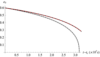
Figure 1: (color online). Comparison of the analytical and numerical results for the evolution of the eccentricity. The initial eccentricity is $e_{0}=0.6$, the masses of binary are $m_{i}=10^{6}(1+z)M_{\odot}$ with redshift $z=1$. The inspiral starts one year before the last stable orbit (LSO) calculated in the Newtonian order which corresponds to the initial frequency $\nu_{0}=8.09\mu\mathrm{Hz}$. In the Newtonian case the dotted black line denotes the analytic, while the gray line the numeric solution. For the 1PN orbital evolution the analytic and numeric solutions are denoted by the dotdashed and red lines, respectively. It can be seen that the perturbative solution is in perfect agreement with the numerical one.

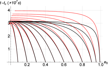
Figure 2: (color online). The time function for various initial eccentricities. Newtonian and 1PN expressions are denoted by solid (black) and dashed (red) lines, respectively. The masses of the components are $m_{i}=10^{6}(1+z)M_{\odot}$ with redshift $z=1$. The inspiral time is set to 1 year before LSO calculated in the Newtonian order.

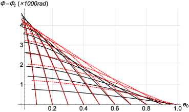
Figure 3: (color online). The phase functions for various initial eccentricities. Newtonian and 1PN expressions are denoted by solid (black) and dashed (red) lines, respectively. The masses of the components are $m_{i}=10^{6}(1+z)M_{\odot}$ with redshift $z=1$. The inspiral time is set to 1 year before LSO calculated in the Newtonian order.

VIII Summary

In our work we have investigated the orbital evolution and emitted radiation of binary systems on eccentric orbits up to 1PN order. Both the time and frequency domain waveforms are presented in a simple form with use the generalized true anomaly parameterization. To express the time dependence of the waveforms the Hansen coefficients were generalized to 1PN accuracy. Moreover, the radiation reaction problem and the evolution of the time and phase functions are given to 1PN accuracy.

Appendix A Tensor spherical harmonics

Following the notation of Mathews the traceless, symmetric and unit basis tensors can be written as

$$t^{\pm 2} = \frac{1}{2}\left(e_{x}\otimes e_{x}-e_{y}\otimes e_{y}\right)\pm\frac{i}{2}\left(e_{x}\otimes e_{y}+e_{y}\otimes e_{x}\right),$$

$$t^{\pm 1} = \mp\frac{1}{2}\left(e_{x}\otimes e_{z}+e_{z}\otimes e_{x}\right)-\frac{i}{2}\left(e_{y}\otimes e_{z}+e_{z}\otimes e_{y}\right),$$

$$t^{0} = \frac{1}{\sqrt{6}}\left(-e_{x}\otimes e_{x}-e_{y}\otimes e_{y}+2e_{z}\otimes e_{z}\right).$$ (76)

The scalar harmonic tensors on this basis are given by

$$T^{2l^{\prime},lm}=\underset{m^{\prime}=-l^{\prime}}{\overset{l^{\prime}}{\sum}}\underset{m^{\prime\prime}=-2}{\overset{2}{\sum}}(l^{\prime}2m^{\prime}m^{\prime\prime},lm)Y^{l^{\prime}m^{\prime}}t^{m^{\prime\prime}},$$ (77)

where $(l^{\prime}2m^{\prime}m^{\prime\prime},lm)$ denotes the Clebsch-Gordan coefficients and $Y^{lm}$ is the conventional spherical harmonic. Then the electric and magnetic tensor harmonics can be expresssed as

$$T^{E2,lm} = \sqrt{\frac{l(l+1)}{2(2l+1)(2l+3)}}T^{2\text{ }l+2,lm}+\sqrt{\frac{3(l-1)(l+2)}{(2l+1)(2l+3)}}T^{2\text{ }l,lm}$$ (78)

$$+\sqrt{\frac{(l+1)(l+2)}{2(2l-1)(2l+1)}}T^{2\text{ }l-2,lm},$$

$$T^{B2,lm} = -i\sqrt{\frac{l-1}{2l+1}}T^{2\text{ }l+1,lm}-i\sqrt{\frac{l+2}{2l+1}}T^{2\text{ }l-1,lm}.$$ (79)

As an example we consider the tensor harmonics $T^{E2,22}$ and $T^{B2,22}$ appearing in the Newtonian waveform. Using the relationship between the Descartes and spherical polar coordinates,

$$e_{x} = e_{r}\sin\theta\cos\varphi+e_{\theta}\cos\theta\cos\varphi-e_{\varphi}\sin\varphi,$$

$$e_{y} = e_{r}\sin\theta\sin\varphi+e_{\theta}\cos\theta\sin\varphi+e_{\varphi}\cos\varphi,$$

$$e_{z} = e_{r}\cos\theta-e_{\theta}\sin\theta,$$ (80)

the tensor harmonics have the form

$$T^{E2,22} = \frac{1}{8}\sqrt{\frac{5}{2\pi}}[\left(1+\cos^{2}\theta\right)h_{+}+2i\cos\theta h_{\times}]e^{2i\varphi},$$ (81)

$$T^{B2,22} = -\frac{1}{16}\sqrt{\frac{5}{2\pi}}[\left(3+\cos 2\theta\right)h_{\times}-4i\cos\theta h_{+}]e^{2i\varphi},$$ (82)

where $h_{+}=e_{\theta}\otimes e_{\theta}-e_{\varphi}\otimes e_{\varphi}$ and $h_{\times}=e_{\theta}\otimes e_{\varphi}+e_{\varphi}\otimes e_{\theta}$ are the two independent polarizations. The tensor spherical harmonics up to 2PN are given in Tessmer2 .

Appendix B Orbital parameters of the 1PN dynamics

The orbital parameters up to 1PN order are given by DD

$$n =\frac{\left(-A\right)^{3/2}}{B}\mathbf{,}$$

$$a_{R} =-\frac{B}{A}+\frac{D}{2C_{0}}\mathbf{,}$$

$$e_{t} =\left[1-\frac{A}{B^{2}}\left(C-\frac{BD}{C_{0}}\right)\right]^{1/2}\mathbf{,}$$

$$e_{R} =\left(1-\frac{AD}{2BC_{0}}\right)e_{t}\mathbf{,}$$

$$e_{\theta} =\left(1+\frac{AD}{BC_{0}}-\frac{AI}{BH}\right)e_{t}\mathbf{,}$$

$$k =\frac{3Gm}{a_{r}(1-e_{R}^{2})},$$ (83)

with the quantities $A-K$ are

$$A =\frac{2E}{\mu}\left(1+\frac{3}{2}\left(3\eta-1\right)\frac{E}{\mu c^{2}}\right)\mathbf{,}$$

$$B =GM\left(1+\left(7\eta-6\right)\frac{E}{\mu c^{2}}\right)\mathbf{,}$$

$$C =-\frac{J^{2}}{\mu^{2}}\left(1+2\left(3\eta-1\right)\frac{E}{\mu c^{2}}\right)+\left(5\eta-10\right)\frac{G^{2}M^{2}}{c^{2}}\mathbf{,}$$

$$D =\left(-3\eta+8\right)\frac{GMJ^{2}}{\mu^{2}c^{2}}\mathbf{,}$$

$$H =\frac{J}{\mu}\left(1+\left(3\eta-1\right)\frac{E}{\mu c^{2}}\right)\mathbf{,}$$

$$I =\left(2\eta-4\right)\frac{GMJ}{\mu c^{2}}\mathbf{,}$$

$$K =\frac{J}{\mu\left(\frac{J^{2}}{\mu^{2}}-\frac{6G^{2}M^{2}}{c^{2}}\right)^{1/2}}.$$ (84)

Appendix C Hansen coefficients

The Hansen coefficients are important functions of the celestial mechanics which are known for more than 100 years. The expansion of Hansen-coefficients is

$$\left(\frac{r}{a}\right)^{n}\exp(im\phi)=\overset{\infty}{\underset{k=-\infty}{\sum}}X_{k}^{n,m}\exp(ik\mathcal{M}),$$ (85)

where $r$ is the relative distance, $a$ is the semimajor axis, $\phi$ is the true anomaly and $\mathcal{M}$ is the mean anomaly using by the standard notations of celestial mechanics. The coefficients $X_{k}^{n,m}$ are called the Hansen-coefficients. Here the constants $n$ and $m$ are integers. The Fourier series representation of the Hansen coefficients is

$$X_{k}^{n,m}=\frac{1}{2\pi}\underset{-\pi}{\overset{\pi}{\int}}\left(\frac{r}{a}\right)^{n}\exp(im\phi-ik\mathcal{M})d\mathcal{M}.$$ (86)

The integrand can be transformation to other argument, specifically the eccentric and true anomalies with the use of the leading order Kepler-equation,

$$\frac{d\mathcal{M}}{du} = 1-e\cos u,$$ (87)

$$\frac{d\mathcal{M}}{dv} = \frac{\left(1-e^{2}\right)^{3/2}}{\left(1+e\cos\phi\right)^{2}}.$$ (88)

We introduce the complex variables $x=\exp i\phi$ and $y=\exp iu$ ($z=\exp i\mathcal{M}$ for the contour integral), then the relationship between the eccentric and true anomalies (Erdi ) with $x$ and $y$ complex variables is

$$\frac{x-1}{x+1}=\frac{1+\beta}{1-\beta}\frac{y-1}{y+1},$$ (89)

and one gets for the variable $x$

$$\exp i\phi=y(1-\beta y^{-1})(1-\beta y)^{-1},$$ (90)

and the mean anomaly $\mathcal{M}$

$$\frac{d\mathcal{M}}{du} = \frac{r}{a}=\left(1+\beta^{2}\right)^{-1}(1-\beta y)(1-\beta y^{-1}),$$ (91)

$$\exp i\mathcal{M} = y\exp\left[-\frac{e}{2}\left(y-y^{-1}\right)\right].$$ (92)

The integrand with eccentric anomaly $u$ is given as

$$X_{k}^{n,m} = \frac{\left(1+\beta^{2}\right)^{-n-1}}{2\pi}\underset{-\pi}{\overset{\pi}{\int}}y^{m-k}(1-\beta y^{-1})^{n+m+1}$$ (93)

$$\times(1-\beta y)^{n-m+1}\exp\left[\frac{ke}{2}\left(y-y^{-1}\right)\right]du.$$

The integral can be extended to infinity as a series of the Bessel functions

$$X_{k}^{n,m}=(1+\beta^{2})^{-n-1}\overset{\infty}{\underset{p=-\infty}{\sum}}E_{k-p}^{n,m}J_{p}(ke).$$ (94)

The coefficients $E_{l}^{n,m}$ for $l\geqq m$ and $E_{-l}^{n,-m}$ for $l<m$ can be expressed by the hypergeometric function $F(a,b;c;d)$ as

$$E_{l}^{n,m} = \left(-\beta\right)^{l-m}\binom{n-m+1}{l-m}$$ (95)

$$\times F(l-n-1,-m-n-1;l-m+1;\beta^{2}).$$

The first description of this formula was given by Hill Plummer . The other representation of the Hansen coefficients can be found in the work of Tisserand on celestial mechanics from 1889,

$$X_{k}^{n,m}=\frac{\left(-\beta\right)^{\left|k-m\right|}}{(1+\beta^{2})^{n+1}}\overset{\infty}{\underset{s=0}{\sum}}\mathcal{P}_{s}\mathcal{Q}_{s}\beta^{2s},$$ (96)

where

$$\mathcal{P}_{s} = \left\{\begin{array}[]{l}P_{s+k-m}\qquad k\geqq m\\ P_{s}\qquad\qquad k<m\end{array}\right\},$$ (99)

$$\mathcal{Q}_{s} = \left\{\begin{array}[]{l}Q_{s}\qquad\qquad k\geqq m\\ Q_{s+m-k}\qquad k<m\end{array}\right\},$$ (102)

and

$$P_{s} = \overset{s}{\underset{r=0}{\sum}}\binom{n-m+1}{s-r}\frac{1}{r!}\left(\frac{kr}{2\beta}\right)^{r},$$ (103)

$$Q_{s} = \overset{s}{\underset{r=0}{\sum}}\binom{n+m+1}{s-r}\frac{1}{r!}\left(-\frac{kr}{2\beta}\right)^{r}.$$ (104)

Appendix D Leading and half order waveforms

The leading order waveform with the true anomaly $\phi$ due to Einstein quadrupole formula are (the notation of ref. mikoczi for azimuthal polar angle is $\gamma=\Phi$)

$$h_{+}^{N}(\phi) = \frac{1}{1-e^{2}}\sum_{m=0}^{5}\left(c_{m}^{N+}\cos m\phi+s_{m}^{N+}\sin m\phi\right),$$ (105)

$$h_{\times}^{N}(\phi) = \frac{1}{1-e^{2}}\sum_{m=0}^{5}\left(c_{m}^{N\times}\cos m\phi+s_{m}^{N\times}\sin m\phi\right),$$ (106)

where

$$c_{0}^{N+} =-\frac{e^{2}}{2}(1+3\cos 2\Phi-2\cos 2\Theta\sin^{2}\Phi), c_{0}^{N\times} =2e^{2}\cos\Theta\sin 2\Phi,$$

$$c_{1}^{N+} =\frac{e}{2}(-1+\cos 2\Theta-5(1+\cos^{2}\Theta)\cos 2\Phi), c_{1}^{N\times} =5e\cos\Theta\sin 2\Phi,$$

$$c_{2}^{N+} =-(3+\cos 2\Theta)\cos 2\Phi, c_{2}^{N\times} =4\cos\Theta\sin 2\Phi,$$

$$c_{3}^{N+} =-\frac{e}{4}(3+\cos 2\Theta)\cos 2\Phi, c_{3}^{N\times} =e\cos\Theta\sin 2\Phi,$$

$$s_{1}^{N+} =-\frac{5e}{4}(3+\cos 2\Theta)\sin 2\Phi, s_{1}^{N\times} =-5\cos\Theta\cos 2\Phi,$$

$$s_{2}^{N+} =-(3+\cos 2\Theta)\sin 2\Phi, s_{2}^{N\times} =-4\cos\Theta\cos 2\Phi,$$

$$s_{3}^{N+} =-\frac{e}{4}(3+\cos 2\Theta)\sin 2\Phi, s_{3}^{N\times} =-e\cos\Theta\cos 2\Phi.$$ (107)

The half order waveforms (denoted by the superscript $H$) are

$$h_{+}^{H}(\phi) = \frac{16}{\left(1-e^{2}\right)^{3/2}}\sum_{m=0}^{5}\left(c_{m}^{+}\cos m\phi+s_{m}^{+}\sin m\phi\right),$$ (108)

$$h_{\times}^{H}(\phi) = \frac{8}{\left(1-e^{2}\right)^{3/2}}\sum_{m=0}^{5}\left(c_{m}^{\times}\cos m\phi+s_{m}^{\times}\sin m\phi\right),$$ (109)

where

$$c_{0}^{H+} = -e\left(2\left(-11+2e^{2}+\left(-1+6e^{2}\right)\cos 2\Theta\right)\sin\Theta\sin\Phi-2e^{2}(5\sin\Theta+\sin 3\Theta)\sin 3\Phi\right),$$

$$c_{1}^{H+} = -\frac{1}{4}\left(2\left(-44-19e^{2}+\left(-4+39e^{2}\right)\cos 2\Theta]\right)\sin\Theta\sin\Phi-35e^{2}(5\sin\Theta+\sin 3\Theta)\sin 3\Phi\right),$$

$$c_{2}^{H+} = e((23\sin\Theta-5\sin 3\Theta)\sin\Phi+15(5\sin\Theta+\sin 3\Theta)\sin 3\Phi),$$

$$c_{3}^{H+} = -\frac{1}{4}\left(e^{2}(-23\sin\Theta+5\sin 3\Theta)\sin\Phi-2\left(18+7e^{2}\right)(5\sin\Theta+\sin 3\Theta)\sin 3\Phi\right),$$

$$c_{4}^{H+} = 5e(5\sin\Theta+\sin 3\Theta)\sin 3\Phi,$$

$$c_{5}^{H+} = \frac{3}{4}e^{2}(5\sin\Theta+\sin 3\Theta)\sin 3\Phi,$$

$$s_{1}^{H+} = -\frac{1}{2}\cos\Phi\left(\left(42-72e^{2}+175e^{2}\cos 2\Phi\right)\sin\Theta+\left(2-32e^{2}+35e^{2}\cos 2\Phi\right)\sin 3\Theta\right),$$

$$s_{2}^{H+} = -e((23\sin\Theta-5\sin 3\Theta)\cos\Phi+15(5\sin\Theta+\sin 3\Theta)\cos 3\Phi),$$

$$s_{3}^{H+} = -\frac{1}{4}\left(e^{2}(23\sin\Theta-5\sin 3\Theta)\cos\Phi+2\left(18+7e^{2}\right)(5\sin\Theta+\sin 3\Theta)\cos 3\Phi\right),$$

$$s_{4}^{H+} = -5e(5\sin\Theta+\sin 3\Theta)\cos 3\Phi,$$

$$s_{5}^{H+} = -\frac{3}{4}e^{2}(5\sin\Theta+\sin 3\Theta)\cos 3\Phi.$$ (110)

Appendix E 1PN waveform

E.1 The coefficients proportional to $\cos m\phi$

There are coefficients proportional to $\cos m\tilde{\phi}$ and $\sin m\tilde{\phi}$ in the 1PN waveform, Eq. (17). Coefficients for $\cos 4\tilde{\phi}$ and $\sin 4\tilde{\phi}$ are (we have introduced the shorthand notations $c_{m\Phi}=\cos m\Phi$, $s_{m\Phi}=\sin m\Phi$, $c_{m\Theta}=\cos m\Theta$, $s_{m\Theta}=\sin m\Theta$, $G_{\Theta}=-5+4c_{2\Theta}+c_{4\Theta}$ and $\lambda_{\eta}=-1+3\eta$. For example, $s_{3(c4)}^{+}$ mean plus polarization, proportional to $\sin 3{\phi}$ and proportional to $\sin 4\tilde{\phi}$)

$$c_{4(c4)}^{+} = \frac{1}{32}c_{4\Phi}G_{\Theta}\lambda_{\eta}\eta e^{4},$$

$$c_{4(s4)}^{+} = \frac{1}{32}s_{4\Phi}G_{\Theta}\lambda_{\eta}\eta e^{4},$$

$$c_{3(c4)}^{+} = \frac{55}{256}c_{4\Phi}G_{\Theta}\lambda_{\eta}\eta e^{3},$$

$$c_{3(s4)}^{+} = \frac{55}{256}s_{4\Phi}G_{\Theta}\lambda_{\eta}\eta e^{2},$$

$$c_{2(c4)}^{+} = \frac{125}{192}c_{4\Phi}G_{\Theta}\lambda_{\eta}\eta e^{2},$$

$$c_{2(s4)}^{+} = \frac{125}{192}s_{4\Phi}G_{\Theta}\lambda_{\eta}\eta e^{2},$$

$$c_{1(c4)}^{+} = \frac{1}{768}c_{4\Phi}G_{\Theta}\lambda_{\eta}\eta(764+135e^{2})e,$$

$$c_{1(s4)}^{+} = \frac{1}{768}s_{4\Phi}G_{\Theta}\lambda_{\eta}\eta(764+135e^{2})e,$$

$$c_{0(c4)}^{+} = \frac{1}{192}c_{4\Phi}G_{\Theta}\lambda_{\eta}\eta(64+71e^{2}),$$

$$c_{0(s4)}^{+} = \frac{1}{192}s_{4\Phi}G_{\Theta}\lambda_{\eta}\eta(64+71e^{2}).$$ (111)

The coefficients proportional to $\cos 2\tilde{\phi}$ and $\sin 2\tilde{\phi}$ are

$$c_{3(c2)}^{+} = \frac{1}{64}c_{2\Phi}\left[291+c_{4\Theta}-3\eta(27+c_{4\Theta})+4(19+9\eta)c_{2\Theta}\right]\eta e^{3},$$

$$c_{3(s2)}^{+} = \frac{1}{64}s_{2\Phi}\left[291+c_{4\Theta}-3\eta(27+c_{4\Theta})+4(19+9\eta)c_{2\Theta}\right]\eta e^{3},$$

$$c_{2(c2)}^{+} = -\frac{1}{48}c_{2\Phi}(-983+114e^{2}+375\eta+18e^{2}\eta+c_{4\Theta}(1+6e^{2})\lambda_{\eta}+2c_{2\Theta}(-116-81\eta+6e^{2}(3+\eta)))e^{2}\eta,$$

$$c_{2(s2)}^{+} = -\frac{1}{48}s_{2\Phi}(-983+114e^{2}+375\eta+18e^{2}\eta+c_{4\Theta}(1+6e^{2})\lambda_{\eta}+2c_{2\Theta}(-116-81\eta+6e^{2}(3+\eta)))e^{2}\eta,$$

$$c_{1(c2)}^{+} = \frac{1}{192}c_{2\Phi}(5948+99e^{2}-3012\eta-1089\eta e^{2}-c_{4\Theta}(4+81e^{2})\lambda_{\eta}+4c_{2\Theta}(33e^{2}(-1+\eta)+4(76+81\eta)))e\eta,$$

$$c_{1(s2)}^{+} = \frac{1}{192}s_{2\Phi}(5948+99e^{2}-3012\eta-1089\eta e^{2}-c_{4\Theta}(4+81e^{2})\lambda_{\eta}+4c_{2\Theta}(33e^{2}(-1+\eta)+4(76+81\eta)))e\eta,$$

$$c_{0(c2)}^{+} = \frac{1}{48}c_{2\Phi}(508+e^{2}(353-465\eta)-228\eta-c_{4\Theta}(-4+19e^{2})\lambda_{\eta}+2c_{2\Theta}(52+60\eta+e^{2}(14+57\eta)))\eta,$$

$$c_{0(s2)}^{+} = \frac{1}{48}s_{2\Phi}(508+e^{2}(353-465\eta)-228\eta-c_{4\Theta}(-4+19e^{2})\lambda_{\eta}+2c_{2\Theta}(52+60\eta+e^{2}(14+57\eta)))\eta.$$ (112)

The coefficients without $\tilde{\phi}$ dependence are

$$c_{3}^{+} = -\frac{1}{256}\left[(5-15\eta)c_{4\Theta}+11(-11+\eta)+4(29+\eta)c_{2\Theta}\right]\eta e^{3},$$

$$c_{2}^{+} = \frac{5}{64}\left[37+4(-9+\eta)c_{2\Theta}-7\eta+\lambda_{\eta}c_{4\Theta}\right]e^{2}\eta,$$

$$c_{1}^{+} = \frac{1}{256}(1196+675e^{2}-196\eta-265e^{2}\eta+c_{4\Theta}(-4+39e^{2})\lambda_{\eta}+4c_{2\Theta}(-300+52\eta+e^{2}(-159+37\eta)))e\eta,$$

$$c_{0}^{+} = \frac{1}{64}\eta(363-50e^{2}-73\eta-10e^{2}\eta+c_{4\Theta}(-1+6e^{2})\lambda_{\eta}+c_{2\Theta}(-364-8e^{2}(-7+\eta)+76\eta)).$$ (113)

E.2 Coefficients proportional to $\sin m\phi$

The coefficients proportional to $\cos 4\tilde{\phi}$ and $\sin 4\tilde{\phi}$ are

$$s_{4(c4)}^{+} = -\frac{1}{32}s_{4\Phi}G_{\Theta}\lambda_{\eta}\eta e^{4},$$

$$s_{4(s4)}^{+} = \frac{1}{32}c_{4\Phi}G_{\Theta}\lambda_{\eta}\eta e^{4},$$

$$s_{3(c4)}^{+} = -\frac{25}{128}s_{4\Phi}G_{\Theta}\lambda_{\eta}\eta e^{3},$$

$$s_{3(s4)}^{+} = \frac{25}{128}c_{4\Phi}G_{\Theta}\lambda_{\eta}\eta e^{3},$$

$$s_{2(c4)}^{+} = -\frac{15}{32}s_{4\Phi}G_{\Theta}\lambda_{\eta}\eta e^{2},$$

$$s_{2(s4)}^{+} = -\frac{15}{32}c_{4\Phi}G_{\Theta}\lambda_{\eta}\eta e^{2},$$

$$s_{1(c4)}^{+} = \frac{1}{128}G_{\Theta}s_{4\Phi}\lambda_{\eta}(52+9e^{2})\eta e,$$

$$s_{1(s4)}^{+} = -\frac{1}{128}G_{\Theta}c_{4\Phi}\lambda_{\eta}(52+9e^{2})\eta e.$$ (114)

The coefficients proportional to $\cos 2\tilde{\phi}$ and $\sin 2\tilde{\phi}$ (coefficients of $\sin m\phi$) are

$$s_{3(c2)}^{+} = \frac{1}{64}s_{2\Phi}(-293-92c_{2\Theta}+c_{4\Theta}+3\eta(29+4c_{2\Theta}-c_{4\Theta}))\eta e^{3},$$

$$s_{3(s2)}^{+} = -\frac{1}{64}c_{2\Phi}(-293-92c_{2\Theta}+c_{4\Theta}+3\eta(29+4c_{2\Theta}-c_{4\Theta}))\eta e^{3},$$

$$s_{2(c2)}^{+} = \frac{1}{16}s_{2\Phi}(-259+81\eta+c_{4\Theta}(-3+2e^{2})\lambda_{\eta}+2e^{2}(19+3\eta)+4c_{2\Theta}(2(-10+\eta)+e^{2}(3+\eta)))\eta e^{2},$$

$$s_{2(s2)}^{+} = -\frac{1}{16}s_{2\Phi}(-259+81\eta+c_{4\Theta}(-3+2e^{2})\lambda_{\eta}+2e^{2}(19+3\eta)+4c_{2\Theta}(2(-10+\eta)+e^{2}(3+\eta)))\eta e^{2},$$

$$s_{1(c2)}^{+} = \frac{1}{64}s_{2\Phi}(-900+204\eta+5c_{4\Theta}(-4+3e^{2})\lambda_{\eta}+11e^{2}(1+21\eta)+4c_{2\Theta}(-4(17+\eta)+e^{2}(1+19\eta)))\eta e,$$

$$s_{1(s2)}^{+} = -\frac{1}{64}s_{2\Phi}(-900+204\eta+5c_{4\Theta}(-4+3e^{2})\lambda_{\eta}+11e^{2}(1+21\eta)+4c_{2\Theta}(-4(17+\eta)+e^{2}(1+19\eta)))\eta e.$$ (115)

The coefficients proportional to $\cos 4\tilde{\phi}$ and $\sin 4\tilde{\phi}$ are (we have introduced the notation $H_{\Theta}=c_{\Theta}-c_{3\Theta}$)

$$c_{4(c4)}^{\times} = \frac{1}{4}s_{4\Phi}H_{\Theta}\lambda_{\eta}\eta e^{4},$$

$$s_{4(c4)}^{\times} = -\frac{1}{4}s_{4\Phi}H_{\Theta}\lambda_{\eta}\eta e^{4},$$

$$c_{3(c4)}^{\times} = \frac{55}{64}s_{4\Phi}H_{\Theta}\lambda_{\eta}\eta e^{3},$$

$$s_{3(c4)}^{\times} = -\frac{55}{64}c_{4\Phi}H_{\Theta}\lambda_{\eta}\eta e^{3},$$

$$c_{2(c4)}^{\times} = \frac{125}{48}s_{4\Phi}H_{\Theta}\lambda_{\eta}\eta e^{2},$$

$$s_{2(c4)}^{\times} = -\frac{125}{48}c_{4\Phi}H_{\Theta}\lambda_{\eta}\eta e^{2},$$

$$c_{1(c4)}^{\times} = \frac{1}{182}s_{4\Phi}H_{\Theta}\lambda_{\eta}\eta(764+135e^{2})e,$$

$$s_{1(c4)}^{\times} = -\frac{1}{182}c_{4\Phi}H_{\Theta}\lambda_{\eta}\eta(764+135e^{2})e.$$ (116)

The coefficients proportional to $\cos 2\tilde{\phi}$ and $\sin 2\tilde{\phi}$ are

$$c_{3(c2)}^{\times} = \frac{1}{32}s_{2\Phi}\left[(3-9\eta)c_{3\Theta}+11(-17+3\eta)c_{\Theta}\right]\eta e^{3},$$

$$s_{3(c2)}^{\times} = -\frac{1}{32}c_{2\Phi}\left[(3-9\eta)c_{3\Theta}+11(-17+3\eta)c_{\Theta}\right]\eta e^{3},$$

$$c_{2(c2)}^{\times} = \frac{1}{24}s_{2\Phi}\left[(-17+6e^{2})\lambda_{\eta}c_{3\Theta}+(-625+159\eta+6e^{2}(13+\eta))c_{\Theta}\right]\eta e^{2},$$

$$s_{2(c2)}^{\times} = -\frac{1}{24}c_{2\Phi}\left[(-17+6e^{2})\lambda_{\eta}c_{3\Theta}+(-625+159\eta+6e^{2}(13+\eta))c_{\Theta}\right]\eta e^{2},$$

$$c_{1(c2)}^{\times} = \frac{1}{96}s_{2\Phi}\left[5c_{3\Theta}(-28+9e^{2})\lambda_{\eta}+(3(7+155\eta)e^{2}+4(-931+321\eta))c_{\Theta}\right]\eta e,$$

$$s_{1(c2)}^{\times} = -\frac{1}{96}c_{2\Phi}\left[5c_{3\Theta}(-28+9e^{2})\lambda_{\eta}+(3(7+155\eta)e^{2}+4(-931+321\eta))c_{\Theta}\right]\eta e.$$ (117)

References

• (1) R. M. O’Leary, B. Kocsis, and A. Loeb, Mon. Not. R. Astron. Soc. 395, 2127 (2009).
• (2) B. Kocsis and J. Levin, Phys. Rev. D85, 123005 (2012).
• (3) J. Cuadra, P. J. Armitage, R. D. Alexander, and M. C. Begelman, Mon. Not. R. Astron. Soc. 393, 1423 (2009).
• (4) A. Sesana, Astrophys. J. 719, 851 (2010).
• (5) M. Preto, I. Berentzen, P. Berczik, D. Merritt, and R. Spurzem, J. Phys. Conf. Ser. 154, 012049 (2009).
• (6) U. Löckmann and H. Baumgardt, Mon. Not. R. Astron. Soc. 384, 323 (2008).
• (7) L. Wen, Astrophys. J. 598, 419 (2003).
• (8) L. Hoffman and L. Loeb, Mon. Not. R. Astron. Soc. 377, 957 (2007).
• (9) N. Seto, Phys. Rev. D85, 064037 (2012).
• (10) S. Naoz, B. Kocsis, A. Loeb, and N. Yunes, Astrophys. J. 773, 187 (2013).
• (11) H. Wahlquist, Gen. Relativ. Gravit. 19, 1101 (1987).
• (12) C. Moreno-Garrido, J. Buitrago, and E. Mediavilla, Mon. Not. R. Astron. Soc. 274, 115 (1995).
• (13) B. Mikóczi, B. Kocsis, P. Forgács and M. Vasúth, Phys. Rev. D86, 104027 (2012).
• (14) R. V. Wagoner and C. M. Will Astrophys. J. 210, 764 (1976). err 215, 984 (1977).
• (15) T. Damour and N. Deruelle,  Ann. Inst. Henri Poincaré A 43 , 107 (1985).
• (16) W. Junker and G. Schäfer, Mon. Not. R. Astron. Soc. 254, 146 (1992).
• (17) M. Tessmer and G. Schäfer, Phys. Rev. D82, 1240064 (2010).
• (18) M. Tessmer and G. Schäfer, Ann. Phys. 523, 813 (2011).
• (19) A. Klein, P. Jetzer, Phys. Rev. D81, 124001 (2010).
• (20) Z. Keresztes, B. Mikóczi and L. Á. Gergely, Phys. Rev. D71, 124043 (2005).
• (21) N. Wex, Class. Quantum Grav 12, 983 (1995).
• (22) G. Schäfer, N. Wex, Phys. Lett A 174, 196 (1993), erratum: 177, 461 (1993).
• (23) P. C. Peters, Phys. Rev. 136, B1224 (1954).
• (24) L. Á. Gergely, Z. I. Perjés and M. Vasúth, Astrophys. J. Suppl. 126, 79 (2000).
• (25) H. C. Plummer, An Introductory Treatise On Dynamic Astronomy, Cambridge (1918).
• (26) M. H. Soffel, Relativity in Astrometry, Celestial Mechanics and Geodesy, Springer-Verlag Berlin Heidelberg (1989).
• (27) M. P. Jarnagin, Astron. Papers Am. Eph. Naut. Almanac 18, 36 (1965).
• (28) V. A. Brumberg, Essential Relativistic Celestial Mechanics, Bristol: Adam Hilger (1991).
• (29) J. Mathews J. Soc. Ind. Appl. Math. 10, 768 (1962).
• (30) K. S. Thorne, Rev. Mod. Phys. 52, 299 (1980).
• (31) P. Colwell, Solving Kepler’s Equations. Over three Centuries, Willmann-Bell (1993).
• (32) E. T. Whittaker and G. N. Watson,  A course of modern analysis, University of Cambridge (1927).
• (33) B. Érdi, Mesterséges Holdak mozgása, (in Hungarian), Tankönyvkiadó, Budapest (1989).