Shear instabilities in shallow-water magnetohydrodynamics

Abstract

Within the framework of shallow-water magnetohydrodynamics, we investigate the linear instability of horizontal shear flows, influenced by an aligned magnetic field and stratification. Various classical instability results, such as Høiland’s growth rate bound and Howard’s semi-circle theorem, are extended to this shallow-water system for quite general profiles. Two specific piecewise-constant velocity profiles, the vortex sheet and the rectangular jet, are studied analytically and asymptotically; it is found that the magnetic field and stratification (as measured by the Froude number) are generally both stabilising, but weak instabilities can be found at arbitrarily large Froude number. Numerical solutions are computed for corresponding smooth velocity profiles, the hyperbolic-tangent shear layer and the Bickley jet, for a uniform background field. A generalisation of the long-wave asymptotic analysis of Drazin & Howard (1962) is employed in order to understand the instability characteristics for both profiles. For the shear layer, the mechanism underlying the primary instability is interpreted in terms of counter-propagating Rossby waves, thereby allowing an explication of the stabilising effects of the magnetic field and stratification.

1 Introduction

The interaction of horizontal shear flows and magnetic fields in stably stratified layers is central to many problems in astrophysical fluid dynamics — involving, for example, planetary interiors, stellar radiative zones and accretion discs. An important example of such a flow, which has received considerable attention recently, is that of the solar tachocline (see Hughes, Rosner & Weiss 2007). The tachocline, discovered via helioseismic observations, is a thin layer in the Sun, extending downwards from the (neutrally stable) base of the convective zone to the (stably stratified) top of the radiative interior, characterised by radial velocity shear and also planetary scale horizontal shears, associated with the equator to pole differential rotation of the Sun. Most models of the solar dynamo invoke the tachocline as the site for the storage and generation of the Sun’s strong, predominantly toroidal magnetic field.

Here we are interested in the stability of such shear flows, and how this depends upon the velocity profile, magnetic field strength, and stratification. Specifically, we consider the linear stability of a steady parallel flow and aligned magnetic field, both sheared in the horizontal cross-stream direction, in the inviscid and perfectly conducting limit. In this first study, we consider the case where there is no background rotation. The nonlinear regime of such instabilities typically leads to turbulent flows; these may be important for dynamo action, through some mean-field $\alpha$-effect, and also for the transport of mass and momentum, which can feed back on the large-scale flow.

It is possible to examine the stability of such flows in a continuously stratified three-dimensional setting (e.g., Miura & Pritchett, 1982; Cally, 2003). However, here we adopt the alternative approach of considering the dynamics of a thin fluid layer under the shallow-water approximation, which is valid when the horizontal length scale of the motion is long compared with the depth of the fluid layer, as is typically the case in large-scale astrophysical flows. This leads to a set of two-dimensional partial differential equations, with no explicit dependence on the vertical co-ordinate, which offers a considerable mathematical simplification. Such shallow-water equations capture the fundamental dynamics of density stratification, including gravity waves, and allow the interaction of stratification with horizontal shear flows and magnetic fields to be analysed in the simplest possible setting.

It should be noted that hydrodynamic shallow-water models, which date back to Laplace, are derived by considering a thin fluid layer of constant density bounded below by a rigid medium and above by a fluid of negligible inertia (e.g., Vallis, 2006, §3.1). The corresponding reduction for electrically conducting fluids — the shallow-water magnetohydrodynamic (SWMHD) equations of Gilman (2000) — additionally requires the fluid layer to be a perfect conductor, and to be bounded above and below by perfect conductors. There are few direct astrophysical analogues for such a configuration. However, we can borrow an important idea from planetary atmospheric dynamics, where the hydrodynamic shallow-water equations are widely used to understand waves and instabilities in a continuously stratified atmospheric layer. This is justified because there is a formal mathematical analogy between the linearised equations in the two systems, provided the layer depth in the shallow-water model is taken to be a so-called equivalent depth (e.g., Gill, 1982, §6.11), so that the shallow-water gravity wave speed (in the horizontal) matches that of (the fastest) gravity waves in a continuously stratified layer. We have this analogy in mind throughout this study.

The SWMHD equations have been studied widely in recent years. They have been shown to possess a hyperbolic as well as a Hamiltonian structure (De Sterck, 2001; Dellar, 2002), and to support wave motions such as inertia-gravity waves and Alfvén waves (Schecter et al., 2001; Zaqarashivili et al., 2008; Heng & Spitkovsky, 2009). As reviewed by Gilman & Cally (2007), they have also been used to study the linear instability of shear flows in spherical geometry, often with modelling tachocline instabilities in mind. These previous studies considered basic states that were functions only of latitude, investigating the dependence of the instabilities on the strength and spatial structure of the magnetic field and on a (reduced) gravity parameter (Gilman & Dikpati, 2002; Dikpati et al., 2003).

In contrast to previous investigations of the instabilities of shear flows in SWMHD, which focused on global instabilities in spherical geometry, here we concentrate on local instabilities, with the aim of examining the linear instability problem in a wider context; for this, we consider the problem in planar geometry. We first derive some growth rate bounds and stability criteria, valid for general basic states. We then study how the instability characteristics of prototypical flows are modified by the combined action of magnetic fields and stratification, which, in isolation, are generally thought to be stabilising. The corresponding hydrodynamic problem has a long history, dating back to Rayleigh, and we are able to draw upon ideas and methods from a substantial literature (e.g., Drazin & Reid, 1981; Vallis, 2006).

We start, in §2, by formulating the linear instability problem for plane-parallel basic states with the flow and field dependent on the cross-stream direction. In §3, we derive extensions of classical growth rate bounds, semi-circle theorems, stability criteria, and parity results for modal solutions. In §4, instabilities of piecewise-constant velocity profiles (the vortex sheet and the rectangular jet) with a uniform magnetic field are examined analytically. Analogous smooth profiles (the hyperbolic-tangent shear layer and the Bickley jet) are studied in §5, both numerically and asymptotically, via a generalisation of the long-wave analysis of Drazin & Howard (1962). The primary instability mechanism for shear layers is interpreted in terms of counter-propagating Rossby waves. The results are discussed in §6.

2 Mathematical formulation

2.1 Governing equations

We consider a thin layer of perfectly electrically conducting fluid moving under the influence of gravity. We use a Cartesian geometry, with horizontal coordinates $x$ and $y$, and an upwards pointing coordinate $z$. At time $t$, the fluid, which is taken to be inviscid and of constant density $\rho$, has a free surface at $z=h(x,y,t)$ and is bounded below by a rigid impermeable boundary at $z=-H(x,y)$.

We consider motions with a characteristic horizontal length scale $L_{0}$ that is long compared with a characteristic layer depth $H_{0}$. One can then make a shallow-water reduction in which the vertical momentum balance is taken to be magneto-hydrostatic, and for which the horizontal velocity $\boldsymbol{u}$ and horizontal magnetic field ${\boldsymbol{B}}$ are independent of $z$. When the bottom boundary is perfectly electrically conducting (and is thus a magnetic field line) and the free surface remains a field line, the magnetic shallow-water equations of Gilman (2000) are obtained. These are an extension of the classical shallow-water equations of geophysical fluid dynamics.

We use these equations in non-dimensional form. We denote the characteristic horizontal velocity of the basic state by $U_{0}$, and the characteristic magnetic field strength by $B_{0}$. Non-dimensionalising $x$ and $y$ by $L_{0}$, $t$ by the advective time-scale $L_{0}/U_{0}$, $H$ by $H_{0}$, $h$ by $U_{0}^{2}/g$ (where $g$ is the acceleration due to gravity), velocity by $U_{0}$, and magnetic field by $B_{0}$, the SWMHD equations are

$$\frac{\partial\boldsymbol{u}}{\partial{t}}+\boldsymbol{u}\cdot\nabla\boldsymbol{u} =-\nabla h+M^{2}{\boldsymbol{B}}\cdot\nabla{\boldsymbol{B}},$$ (1a)

$$\frac{\partial{\boldsymbol{B}}}{\partial{t}}+\boldsymbol{u}\cdot\nabla{\boldsymbol{B}} ={\boldsymbol{B}}\cdot\nabla\boldsymbol{u},$$ (1b)

$$F^{2}\frac{\partial{h}}{\partial{t}}+\nabla\cdot\left((H+F^{2}h)\boldsymbol{u}\right) =0,$$ (1c)

where $F=U_{0}/\sqrt{gH_{0}}$ and $M=(B_{0}/\sqrt{\mu\rho})/U_{0}$, with $\mu$ being the permeability of the fluid. In addition to (1$a$–$c$), the shallow-water reduction implies

$$\nabla\cdot\left((H+F^{2}h){\boldsymbol{B}}\right)=0.$$ (2)

However, (2) need not be considered explicitly; if it is satisfied at some initial time, then (1$a$–$c$) guarantee that it remains satisfied for all time.

The system has two non-dimensional parameters. The Froude number $F$ is the ratio of the characteristic horizontal velocity of the basic state to the gravity wave speed $\sqrt{gH_{0}}$ (and is related to the reduced gravity parameter $G$ of Gilman & Dikpati (2002) via $G=F^{-2}$). The parameter $M$ is the ratio of the Alfvén wave speed $B_{0}/\sqrt{\mu\rho}$ to the characteristic horizontal velocity of the basic state. When $H$ is constant and $F\rightarrow 0$, (1c) and (2) become $\nabla\cdot\boldsymbol{u}=0$ and $\nabla\cdot{\boldsymbol{B}}=0$ respectively, and we recover the equations for two-dimensional incompressible magnetohydrodynamics, with $h$ playing the role of pressure. When $M\rightarrow 0$, (1b) decouples from (1$a$–$c$), and we recover the hydrodynamic shallow-water equations; these have a well-known correspondence with two-dimensional compressible hydrodynamics (e.g., Vallis, 2006, §3.1), which we exploit from time to time.

As an example of astrophysical parameter values, we estimate $F$ and $M$ in the solar tachocline, using data from Gough (2007). We set $U_{0}$ to be the equator to pole difference in the zonal velocity, implying $U_{0}\approx 500\,{\rm m\,s^{-1}}$. There is considerable uncertainty in the strength of the magnetic field in the tachocline (Hughes et al., 2007), although a likely range is $10^{3}\,{\rm G}\lesssim B_{0}\lesssim 10^{5}\,{\rm G}$. Then, taking $\rho=210\,{\rm kg\,m^{-3}}$, we find $0.01\lesssim M\lesssim 1$. To estimate $F$, we must choose a gravity wave speed $\sqrt{gH_{0}}$ for the layer. One means of doing this is to take $H_{0}$ to be the depth of the tachocline and to interpret $g$ as a reduced gravity, accounting for the fractional density difference of the overlying fluid, as in Dikpati & Gilman (2001). However, here we pursue the analogy between shallow-water flows and those of a continuously stratified layer with buoyancy frequency $N$ and depth $H_{1}$, and choose $\sqrt{gH_{0}}$ to be the speed of the fastest gravity wave in such a layer, which is $NH_{1}/\pi$ (Gill, 1982, §6.11). Taking $H_{1}\approx 2\times 10^{7}$ m (i.e. $0.03R_{\odot}$, where $R_{\odot}$ is the solar radius) and $N\approx 8\times 10^{-4}\,{\rm s}^{-1}$, which are bulk values that might describe a mode spanning the entire tachocline, gives a gravity wave speed $NH_{1}/\pi=\sqrt{gH_{0}}\approx 5000\,{\rm m\,s^{-1}}$, corresponding to an equivalent depth $H_{0}\approx 50$ km (taking $g\approx 540\,{\rm m\,s^{-2}}$). Again taking $U_{0}\approx 500\,{\rm m\,s^{-1}}$, we thus estimate $F\approx 0.1$, although it is clear that $F$ would be somewhat smaller or larger if one considered motions towards the top of the radiative zone (with stronger stratification) or towards the base of the convection zone (with weaker stratification).

2.2 The linear instability problem

Above a topography of the form $H=H(y)$, we consider a basic state $h=0$, $\boldsymbol{u}=U(y)\boldsymbol{e}_{x}$ and ${\boldsymbol{B}}=B(y)\boldsymbol{e}_{x}$, so that the magnetic field is initially aligned with the flow. We then consider perturbations in $h$, $\boldsymbol{u}=(u,v)$ and ${\boldsymbol{B}}=(b_{x},b_{y})$ to this state of the form

$$\xi(x,y,t)=\mbox{Re}\{\hat{\xi}(y)\exp\left({\rm i}\alpha(x-ct)\right)\},$$ (3)

where $\alpha$ is the (real) wavenumber and $c$ is the (complex) phase speed. Dropping the hatted notation, the linear evolution is described by

$$\left(\frac{\partial}{\partial{t}}+U\frac{\partial}{\partial{x}}\right)u+U^{\prime}v =-\frac{\partial{}h}{\partial{x}}+M^{2}\left(B\frac{\partial{}b_{x}}{\partial{x}}+B^{\prime}b_{y}\right),$$ (4a)

$$\left(\frac{\partial}{\partial{t}}+U\frac{\partial}{\partial{x}}\right)v =-\frac{\partial{h}}{\partial{y}}+M^{2}B\frac{\partial{}b_{y}}{\partial{x}},$$ (4b)

$$\left(\frac{\partial}{\partial{t}}+U\frac{\partial}{\partial{x}}\right)b_{x}+B^{\prime}v =B\frac{\partial{u}}{\partial{x}}+U^{\prime}b_{y},$$ (4c)

$$\left(\frac{\partial}{\partial{t}}+U\frac{\partial}{\partial{x}}\right)b_{y} =B\frac{\partial{v}}{\partial{x}},$$ (4d)

$$F^{2}\left(\frac{\partial}{\partial{t}}+U\frac{\partial}{\partial{x}}\right)h+H\left(\frac{\partial{u}}{\partial{x}}+\frac{\partial{v}}{\partial{y}}\right)+H^{\prime}v =0,$$ (4e)

where a prime denotes differentiation. Eliminating for $v$, we obtain

$$\left(\frac{S^{2}(Hv)^{\prime}}{H(U-c)^{2}K^{2}}\right)^{\prime}-\left(\frac{\alpha^{2}S^{2}}{H(U-c)^{2}}-\frac{U^{\prime}}{H(U-c)}\left(\frac{S^{2}}{(U-c)^{2}K^{2}}\right)^{\prime}+\frac{Q^{\prime}S^{2}}{(U-c)^{3}K^{2}}\right)Hv=0,$$ (5)

where $Q=-U^{\prime}/H$ is the background potential vorticity, and

$$S^{2}(y)=(U(y)-c)^{2}-M^{2}B^{2}(y),\qquad K^{2}(y)=1-F^{2}S^{2}(y).$$ (6)

Following Howard (1961), under the transformation $Hv=(U-c)G$, equation (5) becomes

$$\left(\frac{S^{2}}{K^{2}}\frac{G^{\prime}}{H}\right)^{\prime}-\frac{\alpha^{2}S^{2}}{H}G=0.$$ (7)

We shall use this more compact form for the remainder of this study. In the non-magnetic shallow-water limit ($M=0$), (5) reduces to equation (3.4) of Balmforth (1999). In the two-dimensional incompressible magnetohydrodynamic limit ($F=0$ and $H=1$), (7) reduces to equation (3.5) of Hughes & Tobias (2001).

We shall consider (7) in either an unbounded domain, for which $|G|\rightarrow 0$ as $|y|\rightarrow\infty$, or in a bounded domain with rigid side walls, where $G=0$ and hence $b_{y}=0$ via (4d). Either way, for given real $\alpha$, (7) is then an eigenvalue problem for the unknown phase speed $c=c_{r}+{\rm i}c_{i}$. We will focus on instabilities, i.e. $c_{i}\neq 0$, in which case (7) has no singularities for real values of $y$. Since the transformation $\alpha\rightarrow-\alpha$ leaves (7) unchanged, we may take $\alpha\geq 0$ without loss of generality. Instability then occurs if $c_{i}>0$, with growth rate $\alpha c_{i}$.

3 General theorems

In this section we derive three results that hold for general shear flows $U(y)$: two provide bounds on the growth rate of any instability, whereas the third concerns implications of the parity of the basic state flow.

3.1 Growth rate bound

A bound on the instability growth rate may be obtained by calculating the rate of change of the total disturbance energy using the combination

$$Hu^{*}\times\eqref{ch3:linear-equ1a}+Hv^{*}\times\eqref{ch3:linear-equ1b}+(M^{2}Hb_{x}^{*})\times\eqref{ch3:linear-equ1c}+(M^{2}Hb_{y}^{*})\times\eqref{ch3:linear-equ1d}+h\times\eqref{ch3:linear-equ1e},$$

where ^∗ denotes complex conjugate. On adopting the form (3) for the perturbations, the real part of this expression gives (on dropping hats)

$$\alpha{}c_{i}\left(H\left(|u|^{2}+|v|^{2}+M^{2}|b_{x}|^{2}+M^{2}|b_{y}|^{2}\right)+F^{2}|h|^{2}\right)=$$ (8)

$$-\mbox{Re}\left(HU^{\prime}\left(vu^{*}-M^{2}b_{x}^{*}b_{y}\right)+M^{2}HB^{\prime}\left(vb_{x}^{*}-u^{*}b_{y}\right)\right)-\mbox{Re}\frac{\mathrm{d}}{\mathrm{d}y}(Hvh^{*}).$$

On integrating over the $y$ domain, employing the boundary condition on $v$, and manipulating the remaining terms on the right hand side using $\pm 2\mbox{Re}(pq^{*})\leq|p|^{2}+|q|^{2}$, we obtain the following bound on the growth rate:

$$\alpha{}c_{i}\leq\frac{1}{2}(\max|U^{\prime}|+M\max|B^{\prime}|).$$ (9)

In the absence of magnetic field, this reduces to the well-known bound in hydrodynamics (Høiland, 1953; Howard, 1961).

3.2 Semi-circle theorems

In a classic paper, Howard (1961) proved that for incompressible hydrodynamic parallel shear flows, the wave speed $c$ of any unstable mode must lie within a semi-circle in the complex plane determined by properties of the basic state flow. Subsequently, semi-circle theorems have been derived for several other hydrodynamical and hydromagnetic systems (e.g., Collings & Grimshaw, 1980; Hayashi & Young, 1987; Shivamoggi & Debnath, 1987; Hughes & Tobias, 2001). In a similar manner, a semi-circle theorem may be derived for the SWMHD system.

Multiplying equation (7) by $G^{*}$, integrating over $y$ and using the boundary condition on $v$ (and hence $G$) gives the relation

$$\int\frac{S^{2}}{K^{2}}\frac{|G^{\prime}|^{2}}{H}\,\mathrm{d}y+\alpha^{2}\int\frac{S^{2}|G|^{2}}{H}\,\mathrm{d}y=0.$$ (10)

The imaginary part of (10) gives

$$c_{i}\int\ (U-c_{r})\chi\,\mathrm{d}y=0,\qquad\textnormal{where}\qquad\chi=\frac{|G^{\prime}|^{2}}{H|K|^{4}}+\alpha^{2}\frac{|G|^{2}}{H}\geq 0.$$ (11)

Equation (11) immediately yields Rayleigh’s result that for unstable modes ($c_{i}>0$), $c_{r}$ lies in the range of $U$ (i.e. $U_{\textnormal{min}}\leq{c_{r}}\leq U_{\textnormal{max}}$, where the subscripts ‘min’ and ‘max’ refer to the minimum and maximum values across the domain).

On using equation (11), the real part of (10) gives

$$(c_{r}^{2}+c_{i}^{2})\int\chi\,\mathrm{d}y=\int\chi\left(U^{2}-M^{2}B^{2}\right)\,\mathrm{d}y-F^{2}\int\frac{|S|^{4}}{H|K|^{4}}|G^{\prime}|^{2}\,\mathrm{d}y,$$ (12)

which implies that

$$0\leq(c_{r}^{2}+c_{i}^{2})\int\chi\,\mathrm{d}y\leq\left(U^{2}-M^{2}B^{2}\right)_{\textnormal{max}}\int\chi\,\mathrm{d}y.$$ (13)

This gives the first semi-circle bound: the complex wave speed $c$ of an unstable eigenfunction must lie within the region defined by

$$c_{r}^{2}+c_{i}^{2}\leq\left(U^{2}-M^{2}B^{2}\right)_{\textnormal{max}}.$$ (14)

The second semi-circle bound is obtained, in the standard manner, from the inequality $0\geq\int(U-U_{\textnormal{max}})(U-U_{\textnormal{min}})\chi\,\mathrm{d}y$. Substituting from (11) and deriving an inequality from (12) leads to the expression

$$0\geq\left(c_{r}^{2}+c_{i}^{2}-(U_{\textnormal{min}}+U_{\textnormal{max}})c_{r}+U_{\textnormal{min}}U_{\textnormal{max}}+M^{2}(B^{2})_{\textnormal{min}}\right)\int\chi\,\mathrm{d}y,$$ (15)

which gives the second semi-circle bound: the speed $c$ of an unstable eigenfunction must lie within the region defined by

$$\left(c_{r}-\frac{U_{\textnormal{min}}+U_{\textnormal{max}}}{2}\right)^{2}+c_{i}^{2}\leq\left(\frac{U_{\textnormal{max}}-U_{\textnormal{min}}}{2}\right)^{2}-M^{2}(B^{2})_{\textnormal{min}}.$$ (16)

Thus, taking these results together, the eigenvalue $c$ of an unstable mode must lie within the intersection of the two semi-circles defined by (14) and (16). In the absence of magnetic field, semi-circle (16) lies wholly within semi-circle (14), and we recover the well-known result of Howard (1961). However, as observed by Hughes & Tobias (2001), who considered the stability of aligned fields and flows in incompressible MHD, for non-zero magnetic field there is the possibility of the two semi-circles overlapping, being disjoint, or indeed ceasing to exist; thus, in addition to giving eigenvalue bounds for unstable modes, these results also provide sufficient conditions for stability. From (14) and (16) it therefore follows that the basic state is linearly stable if any one of the following three conditions is satisfied:

$$M|B|\geq|U|\qquad{\textnormal{everywhere in the domain}};$$ (17)

$$M|B|_{\textnormal{min}}\geq\frac{|U_{\textnormal{max}}-U_{\textnormal{min}}|}{2};$$ (18)

$$\frac{U_{\textnormal{max}}+U_{\textnormal{min}}}{2}-\sqrt{\left(\frac{U_{\textnormal{max}}-U_{\textnormal{min}}}{2}\right)^{2}+M^{2}(B^{2})_{\textnormal{min}}}\geq\sqrt{\left(U^{2}-M^{2}B^{2}\right)_{\textnormal{max}}}.$$ (19)

These results are equivalent to those given by Hughes & Tobias (2001) for incompressible MHD.

A drawback of the above approach is that the bounds do not contain the Froude number $F$. Although it is possible to introduce $F$ into the semi-circle bounds using similar manipulations to that employed by Pedlosky (1964), as shown by Mak (2013) this does not sharpen the bound and we thus omit it.

3.3 Consequences of basic state parity

For the hydrodynamic case, it can be shown that symmetries of the basic state lead to symmetries in the stability problem (Howard, 1963). These results may be generalised to SWMHD if we make the further assumptions that $B^{2}(y)$ and $H(y)$ are even functions about $y=0$.

We first consider the case when $U(y)$ is odd about $y=0$. Equation (7) is unchanged under $c\rightarrow-c$ and $G(y)\rightarrow G(-y)$. Since the equation is also unchanged under $c\rightarrow c^{*}$ and $G\rightarrow G^{*}$, it follows that an eigenfunction with eigenvalue $c=c_{r}+c_{i}$ must be accompanied by eigenfunctions with $c=\pm c_{r}\pm{\rm i}c_{i}$. Thus unstable solutions either have $c_{r}=0$ or are a pair of counter-propagating waves with the same phase speed. As argued by Howard (1963), the symmetry in the basic state implies that there is no preferred direction for wave propagation, consistent with the form of the eigenvalues.

Now consider the case when $U(y)$ is even about $y=0$. Then

$$G_{e}(y)=\frac{1}{2}\left(G(y)+G(-y)\right)\qquad\textnormal{and}\qquad G_{o}(y)=\frac{1}{2}\left(G(y)-G(-y)\right)$$ (20)

are also eigenfunctions of (7). Following Drazin & Howard (1966), if we now take $G_{o}$ multiplied by (7) with $G=G_{e}$ and subtract this from $G_{e}$ multiplied by (7) with $G=G_{o}$, integrating over $-L_{y}\leq y\leq L_{y}$ gives

$$W(G_{e},G_{o})\equiv[G_{e}^{\prime}G_{o}-G_{o}^{\prime}G_{e}]^{+L_{y}}_{-L_{y}}=\textrm{constant}=0,$$ (21)

owing to the imposed boundary conditions on the eigenfunction. The vanishing of the Wronskian $W$ implies that the functions $G_{e}$ and $G_{o}$ are linearly dependent throughout the domain, which is possible only if one of them is identically zero. Thus an unstable eigenfunction corresponding to a particular eigenvalue is either an even or odd function about $y=0$.

4 Piecewise-constant profiles: vortex sheet and rectangular jet

We now consider some simple flow configurations for which the eigenvalue problem (7) can be reduced to an algebraic equation for $c$, from which the conditions for stability can be readily determined. To do this, we take $H=1$ (no topography) and $B=1$ (a uniform magnetic field). We seek solutions of (7) in an unbounded domain, with

$$|G|\rightarrow 0\quad\textnormal{as}\quad|y|\rightarrow\infty.$$ (22)

We consider velocity profiles $U(y)$ that are piecewise constant. If $U(y)$ is discontinuous at $y=y_{0}$, then the eigenfunction $G$ must satisfy two jump conditions at $y=y_{0}$. In the usual way, the (linearised) kinematic boundary condition implies

$$\left[\frac{v}{U-c}\right]^{y_{0}^{+}}_{y_{0}^{-}}=\left[G\right]^{y_{0}^{+}}_{y_{0}^{-}}=0.$$ (23a)

The pressure (or free surface displacement) is also continuous at $$y=y_{0} G y=y_{0}$$. The corresponding condition on is most easily derived by integrating (7) across , yielding

$$\left[\frac{S^{2}}{K^{2}}G^{\prime}\right]^{y_{0}^{+}}_{y_{0}^{-}}=0.$$ (23b)

4.1 Vortex sheet

We first consider the velocity profile

$$U(y)=\begin{cases}+1,&y>0,\\ -1,&y<0.\end{cases}$$

Then, for $y\neq 0$, (7) becomes $G^{\prime\prime}-\alpha^{2}K^{2}G=0$. Using (22) and (23a), we thus find

$$G(y)=\begin{cases}\exp\left(-\alpha{}K_{+}y\right),&y>0,\\ \exp\left(+\alpha{}K_{-}y\right),&y<0,\end{cases}$$ (24)

where

$$K_{\pm}=\sqrt{1-F^{2}\left((1\mp{}c)^{2}-M^{2}\right)},\qquad\mbox{Re}\left(K_{\pm}\right)>0.$$ (25)

The second jump condition (23b) then implies an eigenvalue relation for $c$:

$$\frac{(1-c)^{2}-M^{2}}{K_{+}}+\frac{(1+c)^{2}-M^{2}}{K_{-}}=0.$$ (26)

Note that $c$ is independent of the wavenumber $\alpha$, so any unstable mode with $c_{i}>0$ has an unbounded growth rate as $\alpha\rightarrow\infty$. This is an artefact of considering ideal fluids; viscosity will preferentially suppress small scales and remove this unphysical behaviour.

There are several special cases. When $F=M=0$, we recover the classical Kelvin–Helmholtz instability with $c=\pm{\rm i}$. When $F=0$ but $M\neq 0$, (26) reduces to the incompressible MHD case of Michael (1955), with $c^{2}=-(1-M^{2})$; thus, the Kelvin–Helmholtz instability is stabilised when $M\geq 1$, since the disturbance has to do work to bend the field lines. When $M=0$ but $F\neq 0$, (26) gives the classical hydrodynamic shallow-water dispersion relation, which is analogous to that of two-dimensional compressible hydrodynamics. The Kelvin–Helmholtz instability is stabilised when $F\geq\sqrt{2}$ (Miles, 1958; Bazdenkov & Pogutse, 1983), since the disturbance has to do work to move the free surface against gravity. Thus, increasing $F$ or $M$ in the absence of the other is stabilising.

In the general case where $F$ and $M$ are both non-zero, (26) can be rearranged and squared to yield a quartic equation for $c$:

$$F^{2}c^{4}-2\left(1+F^{2}\left(M^{2}+1\right)\right)c^{2}+\left(M^{2}-1\right)\left(2+F^{2}\left(M^{2}-1\right)\right)=0.$$ (27)

Here we have ignored the degenerate case with $c=0$, which is a solution of (26) when $M=1$. By comparing solutions of (27) with those of (26) found using a Newton iteration method, we find that only two roots of (27) also satisfy (26): these are $c=\pm c_{\rm v}$, where

$$c_{\rm v}={\rm i}\left(\frac{\sqrt{1+4F^{2}+4F^{4}M^{2}}-(1+F^{2}+F^{2}M^{2})}{F^{2}}\right)^{1/2}.$$ (28)

A contour plot of $\mbox{Im}(c_{\rm v})$ is shown in figure 1. From (28), there is instability only if

$$M<1\qquad\textnormal{and}\qquad F<\sqrt{\frac{2}{1-M^{2}}}.$$ (29)

Although increasing $F$ is always stabilising at fixed $M$, the critical value of $F$ above which the flow is stable increases as $M$ increases towards $1$. Thus, although magnetic field and free-surface effects are stabilising in isolation, together they can lead to instabilities at arbitrarily large values of $F$, provided

$$1-\frac{2}{F^{2}}<M^{2}<1.$$ (30)

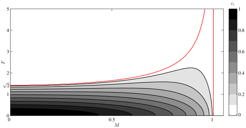
Figure 1: Contours of $\mbox{Im}(c_{\rm v})$, given by expression (28), with stability boundaries (29) in red.

Using an asymptotic analysis, it is possible to investigate these instabilities further at large $F$ and with $M$ just smaller than unity. Rewriting (28) in terms of $1-M^{2}$ and expanding for $|1-M^{2}|\ll 1$, we obtain

$$c_{\rm v}\sim{\rm i}\left(\frac{1-M^{2}}{1+2F^{2}}-\frac{2F^{6}(1-M^{2})^{2}}{(1+2F^{2})^{3}}\right)^{1/2},\qquad|1-M^{2}|\ll 1,$$ (31)

where terms of $O\left((1-M^{2})^{3}\right)$ have been neglected. When $F=O(1)$, the first term on the right-hand side of (31) dominates. However, in the regime of interest (30) with $F^{2}\sim(1-M^{2})^{-1}\gg 1$, the two terms on the right-hand side of (31) have the same order of magnitude, and instead we obtain

$$c_{\rm v}\sim{}{\rm i}\left(\frac{1-M^{2}}{2F^{2}}-\frac{(1-M^{2})^{2}}{4}\right)^{1/2}\quad\textnormal{as}\quad F^{-2}\sim(1-M^{2})\rightarrow 0.$$ (32)

This simple formula is consistent with both stability boundaries in (29), and, as shown in figure 2, closely predicts $c_{i}$ in this weak instability regime, even when $F$ is of order unity. Using (32), it is straightforward to show that $\mbox{Im}(c_{\rm v})$ is maximised when $M^{2}=1-1/F^{2}$, with $c_{\rm v}\sim{\rm i}/(2F^{2})$, so that the growth rate of the most unstable mode decays like $F^{-2}$ in this regime.

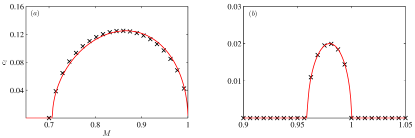
Figure 2: The weak instability regime of the vortex sheet for ($a$) $F=2$, ($b$) $F=5$, as determined directly from (28) (crosses) and from the asymptotic result (32) (line).

4.2 Rectangular jet

We now consider the top-hat velocity profile

$$U(y)=\begin{cases}1,\ &|y|<1,\\ 0,\ &|y|>1.\end{cases}$$ (33)

Then, (7) and (22) imply

$$G=\left\{\begin{array}[]{cc}A_{+}\exp\left(-\alpha{K_{0}}(y-1)\right),&\;\;y>+1,\\ A_{e}\cosh(\alpha{K_{1}}y)+A_{o}\sinh(\alpha{K_{1}}y),&|y|<1,\\ A_{-}\exp\left(+\alpha{K_{0}}(y+1)\right),&\;\;y<-1,\end{array}\right.$$ (34)

for some $A_{+}$, $A_{-}$, $A_{e}$ and $A_{o}$, where

$$K_{0} =\sqrt{1-F^{2}(c^{2}-M^{2})},\quad\textnormal{with}\;\;\mbox{Re}(K_{0})>0\;\;\mbox{for bounded solutions},$$ (35a)

$$K_{1} =\sqrt{1-F^{2}\left((1-c)^{2}-M^{2}\right)},\quad\mbox{with}\;\;-\frac{\pi}{2}<\arg\left(K_{1}\right)\leq\frac{\pi}{2}.$$ (35b)

Here we follow Rayleigh’s formulation (Drazin & Reid, 1981) and consider eigenfunctions that are either even or odd. For the even mode, we set $A_{o}=0$, $A_{+}=A_{-}$ and write $c=c_{e}$. Then (23a,$b$) and (34) give

$$\frac{c_{e}^{2}-M^{2}}{K_{0}}+\frac{(1-c_{e})^{2}-M^{2}}{K_{1}}\tanh(\alpha K_{1})=0.$$ (36)

For the odd mode, we set $A_{e}=0$, $A_{+}=-A_{-}$ and write $c=c_{o}$. Then (23a,$b$) and (34) give

$$\frac{c_{o}^{2}-M^{2}}{K_{0}}+\frac{(1-c_{o})^{2}-M^{2}}{K_{1}}\coth(\alpha{}K_{1})=0.$$ (37)

In contrast to the vortex sheet dispersion relation (26), here $c$ depends upon $\alpha$.

Two special cases may be solved analytically. When $F=M=0$, so that $K_{0,1}=1$, expressions (36) and (37) yield unstable modes with

$$c_{e}=\frac{T+{\rm i}\sqrt{T}}{1+T},\qquad c_{o}=\frac{1+{\rm i}\sqrt{T}}{1+T},\qquad\mbox{where}\;\;T=\tanh\alpha,$$ (38)

so that the flow is unstable for all $\alpha$, with $\mbox{Im}(c)$ approaching a maximum value of $1/2$ as $\alpha\rightarrow\infty$ (Rayleigh, 1878). When $F=0$ but $M\neq 0$, so that $K_{0,1}=1$ again, (36) and (37) yield

$$c_{e}=c_{e}^{(0)}=\frac{T+{\rm i}\sqrt{T-M^{2}(1+T)^{2}}}{1+T},\qquad c_{o}=c_{o}^{(0)}=\frac{1+{\rm i}\sqrt{T-M^{2}(1+T)^{2}}}{1+T}.$$ (39)

(Gedzelman (1973) gave formulae for these two cases (his (3.4) and (3.5)), but both are missing factors of $2$.) Both modes are stable for all $\alpha$ when $M\geq 1/2$; otherwise, both modes are unstable (with the same growth rate) provided that

$$M<M_{c}^{(0)}=\frac{\sqrt{T}}{1+T}\;\Leftrightarrow\;\alpha>\alpha_{c}^{(0)}=\tanh^{-1}\left(\frac{1-2M^{2}-\sqrt{1-4M^{2}}}{2M^{2}}\right).$$ (40)

Thus, the magnetic field introduces a long-wave cutoff.

The other special case with $M=0$ but $F\neq 0$ cannot be solved analytically. Then, (36) and (37) are equivalent to expressions given by Gill (1965), who considered corresponding instabilities for two-dimensional compressible hydrodynamics. An important property is that, at fixed $\alpha$ and $F$, there can be a large number of unstable modes for sufficiently large $F$, which are often interpreted in terms of over-reflection (Takehiro & Hayashi, 1992). This is in contrast to the behaviour at $F=0$, where just two modes exist (one even and one odd), as described by (38).

We generalise these results to cases with $F\neq 0$ and $M\neq 0$ by solving (36) and (37) numerically using a Newton iteration. We start by limiting attention to the smooth extensions of the unstable even and odd modes (38) that exist at $F=0$ and $M=0$, and then tracking these modes over ($M,F$) space; the existence of other unstable modes at high $F$ is discussed in §4.2.5. Contours of $\mbox{Im}(c)$ obtained using this tracking approach are shown in figure 3, for a wide range of $F$, $M$ and $\alpha$. We note that (i) neither mode is unstable for $M>1/2$; (ii) for small $\alpha$, the even mode is stabilised at values of $M$ considerably less than $1/2$; (iii) for small $\alpha$ and small $F$, the odd mode is stabilised at values of $M$ considerably less than $1/2$; (iv) both modes remain unstable for large $F$; (v) when both modes are unstable, the even mode is generally more unstable than the odd mode; (vi) at large $\alpha$, the even and odd modes lead to instabilities of comparable strength, which mimic that of the vortex sheet (cf. figure 1). We now use asymptotic analyses to describe this behaviour in more detail.

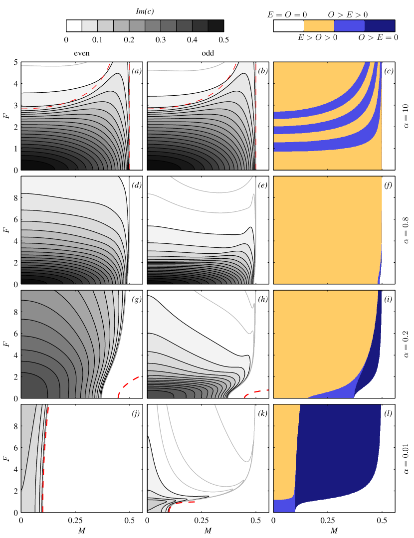
Figure 3: Instability of the rectangular jet. Smooth extensions at fixed $\alpha$ from $(M,F)=(0,0)$ of the unstable modes (38), computed numerically using (36) and (37). Note the different choice of $F$-axis used in the top panels. Left: contours of $\mbox{Im}(c)$ for the even mode. Centre: contours of $\mbox{Im}(c)$ for the odd mode. The black contours are in intervals of $0.025$ from $0.025$ to $0.5$; weak instabilities are shown by the grey contours at $0$, $0.001$, $0.005$ and $0.01$. The $\alpha\gg 1$ stability boundaries (43) are shown as dashed lines in panels ($a,b$). The $\alpha\ll 1$ stability boundaries (48) and (51) are shown as dashed lines in panels ($g,j$) and ($h,k$) respectively. Right: regime diagrams deduced from the left and centre panels, comparing the growth rate of the even mode ($E$) with that of the odd mode ($O$). No regions were found with $E>O=0$.

4.2.1 Instability at large $\alpha$

When $M$ and $F$ are of order unity, $\tanh(\alpha{}K_{1})\approx 1$ when $\alpha\gg 1$ (provided $\alpha\mbox{Re}(K_{1})\gg 1$), so that both (36) and (37) may be approximated by

$$\frac{(\tilde{c}+1/2)^{2}-M^{2}}{\sqrt{1-F^{2}((\tilde{c}+1/2)^{2}-M^{2})}}+\frac{(\tilde{c}-1/2)^{2}-M^{2}}{\sqrt{1-F^{2}\left((\tilde{c}-1/2)^{2}-M^{2}\right)}}=0,$$ (41)

where $\tilde{c}=c_{e}-1/2$ or $\tilde{c}=c_{o}-1/2$. This dispersion relation is similar in form to that for the vortex sheet (26), and a solution may be found in the same way:

$$\tilde{c}={\rm i}\left(\frac{\sqrt{1+F^{2}+F^{4}M^{2}}-(1+F^{2}/4+F^{2}M^{2})}{F^{2}}\right)^{1/2}.$$ (42)

Physically, a sufficiently localised short-wave disturbance sees only one flank of the jet, and thus a vortex sheet instability is obtained to a first approximation. From (42), there is instability only when

$$M<\frac{1}{2}\qquad\textnormal{and}\qquad F<\sqrt{\frac{8}{1-4M^{2}}}.$$ (43)

As shown by the dashed lines in figures 3$a,b$, the conditions (43) approximately bound the region of strong instabilities in ($M,F$) space, even when $\alpha=10$. However, it is also clear that there are additional weak instabilities (shown as grey contours) even when $F>\sqrt{8/(1-4M^{2})}$; the nature of these modes will be discussed in §4.2.5. In contrast, the $M=1/2$ cutoff is robust. Indeed, as is evident from figures 3$d,e$, the magnetic field cutoff stays close to $M=1/2$ (for all $F$) even when $\alpha\approx 1$. For example, at $\alpha=0.8$ and $F=0$, the cutoff $M_{c}\approx 0.490$, using (40).

4.2.2 Instability at small $\alpha$

We consider first the even mode. Assuming that $K_{1}$ remains bounded (which may be confirmed a posteriori), $\tanh(\alpha{}K_{1})\approx\alpha{}K_{1}$ when $\alpha\ll 1$, so that (36) becomes

$$\frac{c_{e}^{2}-M^{2}}{\sqrt{1-F^{2}(c_{e}^{2}-M^{2})}}+\alpha\left((1-c_{e})^{2}-M^{2}\right)=0.$$ (44)

Suppose that $F^{2}=O(1)$. If $M=O(1)$, then $c_{e}=\pm{}M$ at leading order, and the next correction in $\alpha$ is also real: no instabilities are predicted, consistent with figure 3$j$. However, if $M^{2}\sim\alpha\ll 1$, then at leading order, (44) gives

$$c_{e}\sim\pm{\rm i}\sqrt{\alpha-M^{2}}\qquad\textnormal{as}\qquad M^{2}\sim\alpha\rightarrow 0,\quad F^{2}=O(1),$$ (45)

which is consistent with the small $M$ and $\alpha$ limits of (39). Thus a weak magnetic field reduces the strength of the hydrodynamic instability and eventually suppresses it, with instability when

$$M<M_{c}=\alpha^{1/2},\;\mbox{or equivalently when}\;\alpha>\alpha_{c}=M^{2}.$$ (46)

A dependence on $F$ appears only at the next order in $\alpha$, which is why the cutoff in figure 3$j$ is approximately independent of $F$.

To capture the destabilising influence of $F$ apparent in figure 3$g$, the analysis may be extended to larger values of $F$ with $F^{2}\sim\alpha^{-1}\gg 1$. In this case, the square root in (44) also enters the balance at leading order, and we obtain

$$c_{e}\sim{\rm i}\left(\frac{\alpha^{2}F^{2}}{2}-M^{2}+\sqrt{\frac{\alpha^{4}F^{4}}{4}+\alpha^{2}}\right)^{1/2}\qquad\textnormal{as}\qquad M^{2}\sim{}F^{-2}\sim\alpha\rightarrow 0,$$ (47)

which formally reduces to (45) when $F$ is of order unity. Again there is a long-wave cutoff due to the magnetic field, with instability only when

$$M<M_{c}=\frac{\alpha^{2}F^{2}+\sqrt{4\alpha^{2}+\alpha^{4}F^{4}}}{2}\;\;\Leftrightarrow\;\;\alpha>\alpha_{c}=\frac{M^{2}}{\sqrt{1+M^{2}F^{2}}}.$$ (48)

This cutoff, which is shown as a dashed contour in figures 3$g,j$, captures the destabilising influence of $F$. Indeed, in contrast to the result (43) for $\alpha\gg 1$, equation (47) does not predict stabilisation at large $F$ when $\alpha\ll 1$, consistent with the results shown in figures 3$g,j$. The accuracy of this dispersion relation and cutoff when $\alpha\ll 1$ can be seen in figure 4.

In the same $\alpha\ll 1$ limit, the dispersion relation (37) for the odd mode reduces to

$$\frac{\alpha(c_{o}^{2}-M^{2})}{\sqrt{1-F^{2}(c_{o}^{2}-M^{2})}}+\frac{(1-c_{o})^{2}-M^{2}}{1-F^{2}\left((1-c_{o})^{2}-M^{2}\right)}=0.$$ (49)

Suppose that $F^{2}=O(1)$. If $M=O(1)$, then $c_{o}$ is real at the first two orders in $\alpha$: no instabilities are predicted, consistent with figure 3$k$. However, if $M^{2}\sim\alpha\ll 1$, then at leading order, (49) gives

$$c_{o}\sim 1+{\rm i}\left(\frac{\alpha}{\sqrt{1-F^{2}}}-M^{2}\right)^{1/2}\;\textnormal{as}\;\;M^{2}\sim\alpha\rightarrow 0,\;F^{2}=O(1),\;1-F^{2}=O(1).$$ (50)

When $F<1$, again there is a cutoff due to the magnetic field, with instability only when

$$M<M_{c}=\frac{\alpha^{1/2}}{(1-F^{2})^{1/4}},\;\;\mbox{or equivalently when}\;\;\alpha>\alpha_{c}=M^{2}\sqrt{1-F^{2}}.$$ (51)

This cutoff, which is shown as a dashed contour in figures 3$h,k$, captures the sharp destabilising transition as $F\rightarrow 1$, which is particularly evident in figure 3$k$. However, when $F>1$, expression (50) shows that $c_{o}$ always has a positive imaginary part, so that there is no cutoff at small $M$ (when $\alpha\ll 1$). This is clear in figures 3$h,k$, where there are weak instabilities for large $F$ with $M$ close to $1/2$. The absence of a cutoff when $F>1$ is also evident in figure 4$b$.

When $F$ is close to $1$, the asymptotics leading to (50) break down, and one must instead seek solutions with $c=1+O(\alpha^{2/5})$. The resulting (quintic) equation does not admit solutions in closed form (Mak, 2013), although the special case with $F=1$ may be solved exactly, yielding $c_{o}=1+\alpha^{2/5}{\rm e}^{3\pi{\rm i}/5}/2^{1/5}$. Thus $c_{o}$ is independent of $M$ in this regime, consistent with the behaviour shown in the bottom left corners of figures 3$h,k$.

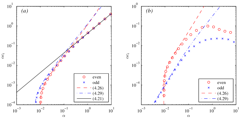
Figure 4: Instability of the rectangular jet at $M=0.1$, for ($a$) $F=0.8$ and ($b$) $F=5$. Shown are the growth rates of the even and odd modes, computed numerically from (36) and (37), and the asymptotic predictions when $\alpha\ll 1$ for the even mode (47) and the odd mode (50). In ($a$), the asymptotic prediction (42) for both modes when $\alpha\gg 1$ is also plotted.

4.2.3 Preferred mode of instability: even versus odd modes

From figure 3, it can be seen that the even mode is more unstable than the odd mode for some parameters but not for others. When $\alpha\gg 1$, both even and odd modes satisfy the same dispersion relation (41) to leading order, as seen in figures 3$a,b$; as shown in figure 3$c$, the even mode is generally more unstable than the odd mode, although this is a weak effect. In contrast, when $\alpha\ll 1$, the odd mode is generally more unstable, as shown in figure 3$l$. In particular, when $F<1$, the odd mode is more unstable (from (45) and (50)) and is unstable over a larger region of parameter space (from (46) and (51)). When $F>1$, again the odd mode is unstable over a larger region of ($M,F$) space; the even mode is stabilised according to (48), whilst the odd mode has no cutoff at small $M$, from (51).

The nature of the transition when $\alpha$ is of order unity can be quantified by performing a small $F$ analysis. We thus write $c=c^{(0)}+F^{2}c^{(1)}+O(F^{4})$ and substitute into (36) for $c_{e}$ and (37) for $c_{o}$. The leading order terms $c_{e}^{(0)}$ and $c_{o}^{(0)}$ are given by (39). In the case where there is instability at leading order, i.e. when (40) is satisfied, we then find

$$\begin{split}&\mbox{Im}\left(c_{e}^{(1)}\right)=a_{e}g,\;\;\;\mbox{Im}\left(c_{o}^{(1)}\right)=a_{o}g,\;\;\;\mbox{where}\;\;g(\alpha,M)=\frac{T^{2}-6T+1}{(T+1)^{2}}+4M^{2},\\ &a_{e}=\frac{T+T^{2}-\alpha(1-T^{2})}{4(1+T)^{2}\sqrt{T-M^{2}(1+T)^{2}}},\;\;\;a_{o}=\frac{T+T^{2}+\alpha T(1-T^{2})}{4(1+T)^{2}\sqrt{T-M^{2}(1+T)^{2}}},\end{split}$$ (52)

and $T=\tanh\alpha$. It is easy to see that $a_{o}>a_{e}>0$ for all $\alpha$, so the behaviour is determined by the sign of $g$. More precisely, the even mode is more unstable (at small $F$) when $4M^{2}<(6T-1-T^{2})/(T+1)^{2}$. This is impossible when $T<3-2\sqrt{2}$, so the odd mode is more unstable at small $F$ when $\alpha<0.1733$, for all $M$. If $T>3-2\sqrt{2}$, then the even mode is more unstable at small $F$ when

$$M<M_{c}=\frac{\sqrt{6T-1-T^{2}}}{2(1+T)}\;\Leftrightarrow\;\alpha<\tanh^{-1}\left(\frac{3-4M^{2}-2\sqrt{2-4M^{2}}}{1+4M^{2}}\right).$$ (53)

For example, when $\alpha=0.2$, the most unstable mode at small $F$ is even when $M<0.159$ and odd when $0.159<M<0.371$ (cf. figure 3$i$); when $\alpha=0.8$, the most unstable mode is even when $M<0.479$ and odd when $0.479<M<0.490$ (cf. figure 3$f$). As $\alpha\rightarrow\infty$, $T\rightarrow 1$ and $M_{c}\rightarrow 1/2$, so there is only a vanishingly thin region close to $M=1/2$ where the odd mode is more unstable at small $F$.

4.2.4 Maximum growth rate

At fixed $F$ and $M$, it is natural to try to find the most unstable wavenumber by maximising $\alpha c_{i}$ with respect to $\alpha$. However, this is not guaranteed to lead to a finite value of $\alpha$: for example, when $F=0$, (39) shows that $c_{i}\rightarrow\sqrt{1-4M^{2}}/2$ as $\alpha\rightarrow\infty$, so provided $M<1/2$ the growth rate $\alpha c_{i}$ increases without bound as $\alpha\rightarrow\infty$. The same phenomenon persists for small $F$, as illustrated in figure 4$a$ at $M=0.1$ and $F=0.8$. However, when $F>\sqrt{8/(1-4M^{2})}$ and $M<1/2$, the asymptotic theory of §4.2.1 for $\alpha\gg 1$ predicts that the flow is stable. In practice, we have seen in figures 3$a,b$ that there are weak instabilities for these parameters, but the growth rates decay sufficiently rapidly with $\alpha$ that a most unstable mode typically occurs at finite $\alpha$, as illustrated in figure 4$b$ at $M=0.1$ and $F=5$. However, we have been unable to find an analytical expression for the most unstable wavenumber in this regime.

4.2.5 Multiple modes of instability at large $F$

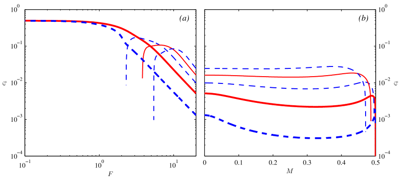
Figure 5: Instability of the rectangular jet at $\alpha=1$, and $M=0$ (left) and $F=20$ (right). Shown is $c_{i}=\mbox{Im}(c)$ computed numerically from (36) and (37). Even modes are shown as solid lines, and odd modes as dashed lines. The unique even and odd modes that smoothly connect to the modes at $(M,F)=(0,0)$ are shown as thicker lines.

In addition to the smooth extensions of the unstable even mode and odd mode that exist at $(M,F)=(0,0)$ (the primary modes), there exist secondary modes of instability for sufficiently large $F$. Instabilities of this type are shown in figure 5. At $M=0$, the first such secondary mode, which is odd, appears close to $F=2.3$; the next secondary mode, which is even, appears close to $F=3.8$. For larger values of $F$, the secondary modes are more unstable than the primary modes; this behaviour persists for $M\neq 0$, as shown in figure 5$b$. Although an asymptotic description of the secondary modes is possible as $F\rightarrow\infty$, the growth rates are relatively small, so these modes are not discussed further.

5 Smooth profiles: hyperbolic-tangent shear layer and Bickley jet

As a model of more realistic velocity profiles, we consider in this section the instabilities of the hyperbolic-tangent shear layer and the Bickley jet. These may be regarded as smooth versions of the piecewise-linear profiles studied in §4. Linear instability calculations involving these two profiles are well documented in a wide variety of contexts (e.g., Lipps, 1962; Howard, 1963; Michalke, 1964; Sutherland & Peltier, 1992; Hughes & Tobias, 2001) and these provide a comparison and check on our results. We again restrict attention (for simplicity) to the case of a uniform background magnetic field, $B(y)\equiv 1$, and with no underlying topography.

5.1 Numerical method

We seek a numerical solution of the eigenvalue equation (7), written as

$$G^{\prime\prime}+\left(\frac{(S^{2})^{\prime}}{S^{2}}-\frac{(K^{2})^{\prime}}{K^{2}}\right)G^{\prime}-\alpha^{2}K^{2}G=0,$$ (54)

where, again, $S^{2}=(U-c)^{2}-M^{2}$ and $K^{2}=1-F^{2}S^{2}$. Although the velocity profiles are defined over the entire real line, we solve (54) on $y\in[-L,L]$, using a shooting method, with matching imposed at $y=0$, employing a generalised Newton method as the root-finding algorithm. Since the solutions decay exponentially as $|y|$ becomes large, namely

$$G\sim\exp\left(-\alpha{}K_{\pm}y\right)\qquad\textnormal{as}\qquad|y|\rightarrow\infty,$$ (55)

where

$$K_{\pm}^{2}=1-F^{2}\left((U_{\pm}-c)^{2}-M^{2}\right),\qquad U_{\pm}=\lim_{y\rightarrow\pm\infty}U(y),$$ (56)

we adopt expression (55) as the boundary condition to be implemented at $y=\pm L$. Since our interest is in instabilities, singularities in the governing equation are avoided. To ensure negligible influence of the finite domain, $L$ is doubled until the computed eigenvalue changes by less than 0.5%. The routines are written in MATLAB, using ode113 as the integrator (an Adams-Bashforth method with adaptive grid). Although the boundary conditions are functions of $c$, changing at every iteration, we generally have no problems with convergence provided that the initial guess is close to the true value. Solutions are initialised from $(M,F)=(0,0)$ at some fixed $\alpha$ using a known numerical result documented in, for example, Drazin & Reid (1981). Runs at new parameter values are then initialised using an estimate for $c$ from previously calculated values at nearby parameters. The Bickley jet is even about $y=0$ and hence the parity result of §3.3 holds — i.e. the eigenfunctions are either even or odd. In this case we need integrate only up to $y=0$, with the imposition of either $G^{\prime}(0)=0$ (even mode) or $G(0)=0$ (odd mode).

5.2 Hyperbolic-tangent shear layer

In this subsection, we consider the basic state velocity defined by

$$U(y)=\tanh y.$$ (57)

From inequality (9) we know that the growth rates $\alpha{}c_{i}$ are bounded above by $|U^{\prime}|_{\mathrm{max}}/2=1/2$; furthermore, from the stability criteria (17) or (18), this profile is stable when $M\geq 1$.

When $M=F=0$, instability exists only when $0<\alpha<1$, with a neutral mode at $\alpha=1$ (e.g., Drazin & Reid, 1981, §31.10). in this case, there is a single primary mode of instability, which may be classified as an inflection-point instability and attributed to interacting Rossby waves supported by the background shear (see, for example, the review by Carpenter et al., 2013). For both two-dimensional compressible hydrodynamics and shallow-water hydrodynamics, there is a secondary mode of instability, first found by Blumen et al. (1975). This has a smaller growth rate and a less pronounced spatial decay than the primary mode. Further, whilst the primary mode has $c_{r}=0$, there are two branches for the secondary mode with equal and opposite (non-zero) phase speeds, consistent with the parity results in §3.3, which ensure that $c=\pm c_{r}+{\rm i}c_{i}$ for unstable modes. The secondary mode can be attributed to interacting gravity waves (e.g., Satomura, 1981; Hayashi & Young, 1987; Takehiro & Hayashi, 1992; Balmforth, 1999) and, indeed, can occur for linear shear flows, explicitly filtering out the possibility of Rossby waves due to a background vorticity gradient. This is consistent with the theorem of Ripa (1983), which states that for instability, either the associated potential vorticity profile possesses an inflection point or $F>1$, both of which encourage instability through interacting waves.

Both modes have been found in our SWMHD system. Figure 6 shows contours of $c_{i}$ over $(M,F)$ space at selected values of $\alpha$ for the profile (57), distinguishing between the primary mode (with $c_{r}=0$, shown as solid contours) and the secondary mode (with $c_{r}\neq 0$, shown as dashed contours). In figure 6$a$, at $\alpha=0.7$, and figure 6$b$, at $\alpha=0.44$ (which is the most unstable mode when $M=F=0$ (Michalke, 1964)), only the primary mode exists. In figure 6$c$, at $\alpha=0.2$, and figure 6$d$, at $\alpha=0.01$, both modes exist, although largely in different parts of $(M,F)$ space. Note that figure 6$d$ and figure 1 are remarkably similar, suggesting that long-wave instabilities for this velocity profile resemble those of the vortex sheet. This will be quantified via a long-wave asymptotic analysis in §5.5, in which we derive the more general result that long-wave instabilities of any shear-layer profile display the characteristics of vortex sheet instabilities.

The growth rate $\alpha c_{i}$ is shown in figure 7 as a function of $\alpha$. It can be seen that the secondary modes generally have weaker growth rates than the primary modes, consistent with the results of Blumen et al. (1975). As we shall see in §5.5, the relation between the two types of unstable modes can be explored in some detail in the long wavelength limit.

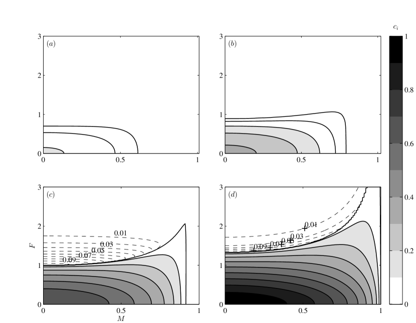
Figure 6: Contours of $c_{i}$ over $(M,F)$ space at ($a$) $\alpha=0.70$, ($b$) $\alpha=0.44$, ($c$) $\alpha=0.20$, ($d$) $\alpha=0.01$. The primary modes (here classified by $|c_{r}|<10^{-3}$) are contoured as solid lines. The secondary modes are contoured as dashed lines.

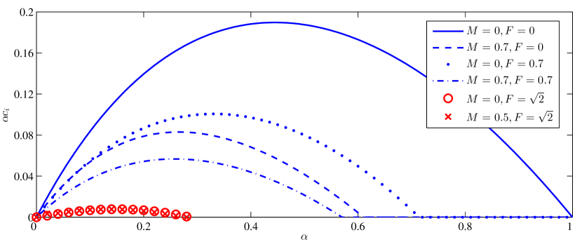
Figure 7: Growth rate versus $\alpha$ at selected parameter values for $U(y)=\tanh y$. The upper four curves are primary modes, the lower two are secondary modes.

5.3 Instability mechanism: Counter-propagating Rossby Waves

As mentioned above, inflection point instabilities can be attributed to interacting Rossby waves supported by the background shear. The constructive interference of a pair of Counter-propagating Rossby Waves (CRWs) has been proposed as the mechanism leading to instability of shear flows in a variety of settings (e.g., Bretherton, 1966; Hoskins et al., 1985; Baines & Mitsudera, 1994; Heifetz et al., 2004; Harnik & Heifetz, 2007). For the SWMHD system, it is therefore natural to enquire how this underlying mechanism is modified by magnetic and shallow-water effects.

Let us first consider the case of $M=0$, $F=0$. The background vorticity profile supports two Rossby waves, propagating in the negative (positive) $x$-direction on the positive (negative) vorticity gradient in $y>0$ ($y<0$). Viewed individually, the Rossby waves are neutral and propagate against the mean flow. If, however, they become phase locked, they can interfere constructively, leading to mutual amplification and hence instability. This is shown schematically in figure 8, where the two Rossby waves are represented as perturbed vorticity contours (or equivalently perturbed material contours) for $y>0$ and $y<0$. The resulting positive and negative vorticity anomalies are also shown. In this configuration, the transverse flow induced by each wave acts to amplify the existing transverse material displacement of the other. There is thus a mutual amplification and instability. This is also consistent with numerical solutions for instabilities of the flow (57) when $M=F=0$; figure 9$a$ shows the vorticity perturbation of the most unstable mode (with $\alpha=0.44$), in agreement with figure 8.

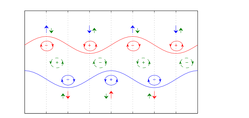
Figure 8: Modified CRW mechanism in schematic form. Shown are two displaced material contours. The associated vorticity anomalies when $M=F=0$ are shown by the closed solid curves; the effect of these on the other contours, leading to instability, is shown by the longer arrows. The closed dashed curves represent the additional vorticity anomalies when $M$ and $F$ are non-zero. The stabilising effect of these, which opposes the driving of the instability, is shown by the shorter arrows.

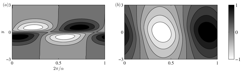
Figure 9: Eigenfunctions of ($a$) vorticity and ($b$) height for the most unstable modes for $U(y)=\tanh y$ at $F=0$, $M=0$.

We now quantify how free-surface and magnetic effects modify this mechanism for SWMHD. We use the SWMHD vorticity equation, which is given by

$$\frac{\mathrm{D}\omega}{\mathrm{D}t}\equiv\frac{\partial\omega}{\partial{}t}+\boldsymbol{u}\cdot\nabla\omega=-(\nabla\cdot\boldsymbol{u})\omega+M^{2}{\boldsymbol{B}}\cdot\nabla{}j+M^{2}(\nabla\cdot{\boldsymbol{B}})j,$$ (58)

where $\omega$ and $j$ are the $z$-components of the vorticity and electric current. Using equations (1c) and (2), (58) can be written as

$$\frac{\mathrm{D}\omega}{\mathrm{D}t}=F^{2}\omega\frac{\mathrm{D}h}{\mathrm{D}t}+F^{2}h\omega\nabla\cdot\boldsymbol{u}+M^{2}(1-F^{2}j){\boldsymbol{B}}\cdot\nabla{}j-M^{2}hj\nabla\cdot{}{\boldsymbol{B}}.$$ (59)

On linearising about the basic state ${\boldsymbol{U}}_{0}=U(y)\boldsymbol{e}_{x}$, ${\boldsymbol{B}}_{0}=\boldsymbol{e}_{x}$, taking modal solutions of the form (3), and noting that $v=(\partial/\partial{}t+U\partial/\partial{}x)\eta$, where $\eta$ is the cross-stream displacement, we obtain the the vorticity budget:

$$\omega=-\eta\Omega^{\prime}+F^{2}h\Omega+M^{2}\frac{j}{U-c},$$ (60)

where $\Omega=-U^{\prime}$ is the basic state vorticity. The three contributions to $\omega$ arise from the advection of the background vorticity and from shallow-water and magnetic effects.

Inspection of figure 6 shows that the instability is most vigorous when $M=F=0$; we therefore expect that the vorticity anomalies from the magnetic and shallow-water effects will be stabilising. The vorticity $\omega$ and the decomposition (60) are shown in figure 10 for a mode at $M=0.25$, $F=0.5$. Even though this eigenfunction results from a calculation with non-zero $F$ and $M$, the $-\eta\Omega^{\prime}$ contribution has the same structure as that of figure 9$a$. The extra contributions from non-zero $F$ and $M$ are shown in figure 10$c,d$; both of these terms are maximised at $y=0$, where they are approximately in phase. Thus, at the simplest level, they lead to the vorticity anomalies shown by the dashed circles in figure 8. The transverse flow induced by these vorticity anomalies counteracts the mutually amplifying transverse flow of the Rossby waves, and is thus stabilising.

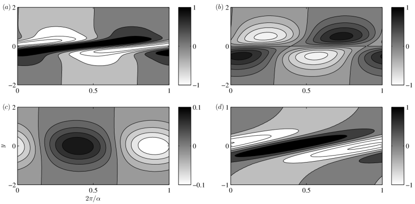
Figure 10: A generic vorticity budget breakdown for the case where neither $F$ nor $M$ is zero; shown here is $F=0.5$ and $M=0.25$, with ($a$) $\omega$, ($b$) $-\eta\Omega^{\prime}$, ($c$) $F^{2}h\Omega$, ($d$) $M^{2}j/(U-c)$. Notice that the vorticity contribution from the magnetic term is substantially larger than that from the shallow-water term.

As a further verification of these ideas, we have also adopted a perturbative approach to the analysis of expression (60), approximating the shallow-water and magnetic contributions using the eigenfunction for $M=F=0$. It can be seen that calculating $F^{2}h\Omega$ using $h$ in figure 9$b$ is consistent with the full linear equations (figure 10$c$). To obtain an estimate of the magnetic contribution, it is necessary to calculate $j$ using the governing equations (4) with the velocity obtained when $M=F=0$. This is slightly more involved than for $h$, but can be shown to provide a vorticity contribution consistent with figure 10$d$ (see Mak 2013).

5.4 Bickley jet

In this subsection we consider the basic state velocity defined by

$$U(y)=\textnormal{sech}^{2}y,$$ (61)

again with $B(y)\equiv 1$. From inequality (9), the growth rate $\alpha{}c_{i}$ is bounded above by $|U^{\prime}|_{\mathrm{max}}/2=2/(3\sqrt{3})$; furthermore, from stability criterion (18), this flow is stable when $M\geq 1/2$. When $M=F=0$, even and odd modes are unstable only in the respective bandwidths $0<\alpha<2$ and $0<\alpha<1$ (e.g., Drazin & Reid, 1981, §31.9).

Figure 11 shows contours of $c_{i}$ over $(M,F)$ space for selected values of $\alpha$. As for figure 6, the eigenvalues are calculated using a mode-tracking procedure, starting from the case of $M=F=0$. The values of $\alpha$ correspond to: (i) the most unstable mode when $M=F=0$ (panels $a$ and $b$); (ii) the mode with highest $c_{i}$ when $M=F=0$ (panels $c$ and $d$); (iii) a long-wave disturbance (panels $e$ and $f$). In all these cases the magnetic field is stabilising. This effect will be quantified later via a long-wave asymptotic analysis.

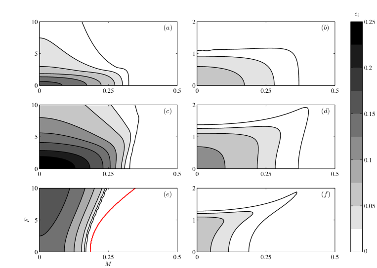
Figure 11: Contours of $c_{i}$ over $(M,F)$ space at selected $\alpha$ for the even (left column) and odd (right column) modes of the Bickley jet, with ($a$) $\alpha=0.9$, ($b$) $\alpha=0.52$, ($c$) $\alpha=0.3$, ($d$) $\alpha=0.23$, ($e,f$) $\alpha=0.05$. The cutoff from the asymptotic result (77) is also plotted in panel ($e$).

Figure 12 shows the growth rate at selected parameter values. In general, the even mode is more unstable than the odd mode. There are isolated regions where the odd mode is more unstable, although these do not necessarily correspond to the regions predicted by the stability analysis for the rectangular jet, described in §4.

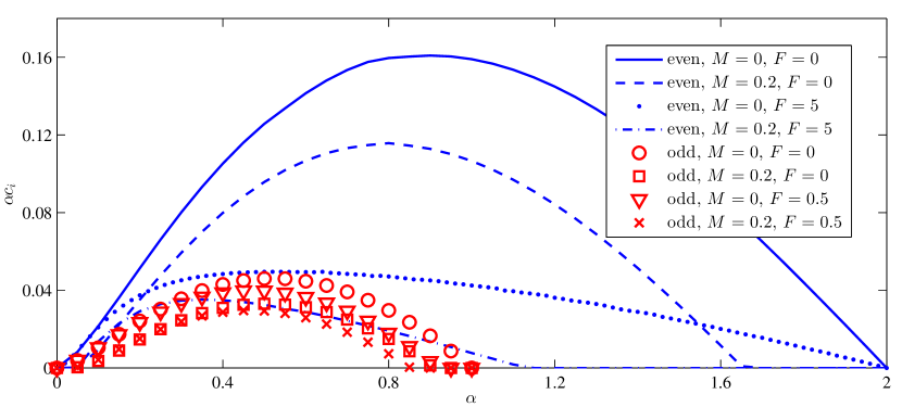
Figure 12: Growth rate of the primary instability of the Bickley jet.

A natural question to ask, prompted by the findings for the shear layer as well as the results for the rectangular jet in §4.2.5, is whether there are additional modes of instability to those shown in figure 12. We have performed a scan over $(M,F)$ space at various values of $\alpha$, with randomly generated initial guesses for $c$ within the smallest rectangle containing the semi-circle (16). A substantial number of computations ($20$ different initialisations at over $200$ different parameter values) were carried out, solving the governing eigenvalue equation with no parity imposed. Other solution branches were found for large $F$ when $\alpha$ is sufficiently large, analogous to the secondary modes for the rectangular jet in §4.2.5. Sample plots of $c_{i}$ and cross-sections of the eigenfunctions for the even modes are shown in figure 13; the results for the odd mode are similar. As in §4.2.5, further secondary modes appear as $F$ increases (figure 13$a$) and the associated growth rates are small (figures 13$a,b$). However, in contrast to the results shown in figure 5 for the rectangular jet, we did not find branch crossings in $c_{i}$ for the Bickley jet; this may occur at higher values of $F$, but computations are demanding since $c_{i}$ becomes increasingly small.

There are two distinctive features of the spatial structure of the eigenfunctions, as shown in figures 13$c,d,e$. First, there is a core region consisting of approximately quantised oscillations: the primary mode has one oscillation, the $n^{\textnormal{th}}$ secondary mode has $n+1$ oscillations. Second, the boundary of the core region is approximately located where $U(y)=c_{r}$. Here the eigenfunctions are highly oscillatory and of larger amplitude, although they are well-resolved in figures 13$c,d,e$.

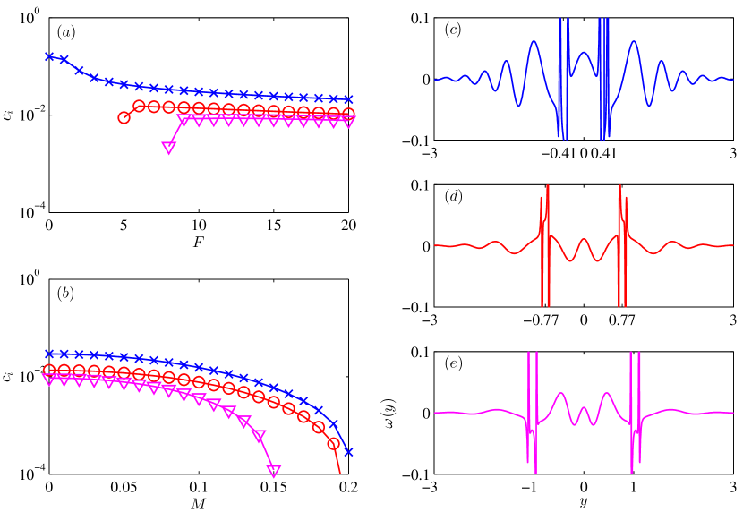
Figure 13: Even mode of the Bickley jet at $\alpha=1$. ($a$) $c_{i}$ as a function of $F$ at $M=0$, $\alpha=1$. ($b$)  $c_{i}$ as a function of $M$ at $F=20$. Crosses show the primary mode, circles and triangles the first two secondary modes. ($c,d,e$) Cross-sections of the vorticity perturbation for $M=0.05$, $F=20$ for the primary and first two secondary modes. The locations where $U=c_{r}$ are labelled on the axes. The spikes reach an amplitude of approximately $0.5$; the display range has been reduced in order that the oscillations within the core are clearly visible.

5.5 Long-wave asymptotics for unbounded smooth profiles

Further understanding of shear flow instabilities in SWMHD can be obtained by generalising the long-wave asymptotic procedure of Drazin & Howard (1962), who considered two-dimensional hydrodynamics. The idea is that, for long-wave disturbances, the leading order behaviour of the instability is determined by $U(y)$ as $|y|\to\infty$, with higher order corrections determined by the flow at finite $y$. In this subsection we extend the formalism of Drazin & Howard (1962) to SWMHD, but with a uniform magnetic field and no topography.

We consider the governing equation (54), written as

$$Z^{2}(G^{\prime\prime}-\alpha^{2}K^{2}G)+(Z^{2})^{\prime}G^{\prime}=0,\qquad Z^{2}=\frac{S^{2}}{K^{2}}.$$ (62)

We assume that $U_{\pm}=U(\pm\infty)$ are well defined and that $U^{\prime}$ (and so $(Z^{2})^{\prime}$) decays sufficiently rapidly as $|y|\to\infty$. Then, on choosing an appropriate frame of reference and suitable normalisation for the basic flow, any velocity profile may be designated as either a shear layer if $U_{\pm}=\pm 1$, or as a jet if $U_{\pm}=0$.

Adopting the same notation as Drazin & Howard (1962), we consider solutions to (62) of the form

$$G(y)=\begin{cases}G_{+}(y)=\chi(y)\exp(-\alpha{K_{+}}y),\ &y>0,\\ G_{-}(y)=\theta(y)\exp(+\alpha{K_{-}}y),\ &y<0,\\ \end{cases}$$ (63)

where $K^{2}_{\pm}=1-F^{2}S^{2}_{\pm}=1-F^{2}\left((U_{\pm}-c)^{2}-M^{2}\right)$. The perturbations must decay as $|y|\to\infty$; hence $\mbox{Re}(K_{\pm})>0$. We consider expansions of the form

$$\chi(y)=\sum^{\infty}_{n=0}(+\alpha)^{n}\chi_{n}(y),\qquad\theta(y)=\sum^{\infty}_{n=0}(-\alpha)^{n}\theta_{n}(y),$$ (64)

with $\chi_{0},\theta_{0}\to\mathrm{constant}\ (\neq 0)$ and $\chi_{n},\theta_{n}\to 0$ as $|y|\to\infty$ $(n\geq 1)$. It turns out to be most convenient to fix $\chi_{0}(\infty)=\theta_{0}(-\infty)=1$, and then to accommodate the necessary degree of freedom in the matching conditions for $G$ at $y=0$, namely $G_{+}(0)=\Gamma{}G_{-}(0)$ and $G_{+}^{\prime}(0)=\Gamma{}G_{-}^{\prime}(0)$ for some constant $\Gamma$. Consistency thus implies

$$G_{+}(0)G_{-}^{\prime}(0)=G_{-}(0)G_{+}^{\prime}(0).$$ (65)

Without loss of generality, we shall focus on the equations for $\chi$; those for $\theta$ follow in a similar fashion. On substituting (63) (with (64)) into (62), equating the coefficients at each order of $\alpha$ gives

$$0 =\left(Z^{2}\chi_{0}^{\prime}\right)^{\prime},$$ (66a)

$$0 =\left(Z^{2}\chi_{1}^{\prime}\right)^{\prime}-K_{+}\left(2Z^{2}\chi_{0}^{\prime}+(Z^{2})^{\prime}\chi_{0}\right),$$ (66b)

$$0 =\left(Z^{2}\chi_{n+2}^{\prime}\right)^{\prime}-K_{+}\left(2Z^{2}\chi_{n+1}^{\prime}+(Z^{2})^{\prime}\chi_{n+1}\right)+Z^{2}(K_{+}^{2}-K^{2})\chi_{n},\ \ n\geq 0.$$ (66c)

Equation (66a) integrates to $Z^{2}\chi_{0}^{\prime}=C$, with the conditions at infinity then giving $C=0$. Thus $\chi_{0}=\textrm{constant}=1$ through our choice of $\chi_{0}(\infty)$. Integration of equations (66$b,c$) then gives, after some algebra,

$$\chi_{1}=\int_{\infty}^{y}\left(1-\frac{Z_{+}^{2}}{Z^{2}}\right)\,\mathrm{d}y_{1},$$ (67)

$$\chi_{2}=\int_{\infty}^{y}\left(\frac{1}{Z^{2}}\int_{\infty}^{y_{1}}(S^{2}-S^{2}_{+})\ \mathrm{d}y_{2}+K_{+}^{2}\int_{\infty}^{y_{1}}\left(1-\frac{Z_{+}^{2}}{Z^{2}}\right)\,\mathrm{d}y_{2}\right)\,\mathrm{d}y_{1}.$$

The matching condition (65) then leads to the result

$$0 =\left(\frac{S_{+}^{2}}{K_{+}}+\frac{S_{-}^{2}}{K_{-}}\right)$$ (68)

$$+\alpha\left(\int_{0}^{\infty}(S^{2}-S_{+}^{2})\,\mathrm{d}y+\int_{-\infty}^{0}(S^{2}-S_{-}^{2})\,\mathrm{d}y\right.$$

$$\left.-\frac{S^{2}_{+}}{K_{+}K_{-}}\int_{-\infty}^{0}\left(1-\frac{S_{-}^{2}}{S^{2}}\right)\mathrm{d}y-\frac{S^{2}_{-}}{K_{+}K_{-}}\int_{0}^{\infty}\left(1-\frac{S_{+}^{2}}{S^{2}}\right)\,\mathrm{d}y\right)+O(\alpha^{2}).$$

On expressing the eigenvalue $c$ as $c=c^{(0)}+\alpha c^{(1)}+\alpha^{2}c^{(2)}+\cdots$, equation (68) then determines the successive $c^{(j)}$.

Although we have focused on the case of a uniform magnetic field, it is possible to include a non-uniform field, subject to imposing conditions analogous to those for $U(y)$. With underlying topography, other assumptions are required (Collings & Grimshaw, 1980).

5.5.1 Shear layers

For a shear layer, $U_{\pm}=\pm 1$, and the leading order term of expression (68) gives

$$\frac{(1-c^{(0)})^{2}-M^{2}}{\sqrt{1-F^{2}\left((1-c^{(0)})^{2}-M^{2}\right)}}+\frac{(1+c^{(0)})^{2}-M^{2}}{\sqrt{1-F^{2}\left((1+c^{(0)})^{2}-M^{2}\right)}}=0.$$ (69)

This is exactly the eigenvalue equation of the vortex sheet (26); hence, for any shear layer, $c\rightarrow c_{\rm v}$, as defined in (28), as $\alpha\rightarrow 0$. This is not surprising; sufficiently long waves see the shear layer as a discontinuity in the flow.

When $F$ is sufficiently large, $c_{\rm v}$ is real (see §4.1). In this case, following Blumen et al. (1975), we calculate $c^{(1)}$ to seek a secondary mode of instability. For the particular case $U(y)=\tanh y$, and after considerable algebra, we obtain

$$c^{(1)}= {\rm i}\frac{\sqrt{F^{2}\left((1-c_{\rm v})^{2}-M^{2}\right)-1}}{4c_{\rm v}^{2}}\frac{(1+c_{\rm v})^{2}-M^{2}}{\sqrt{1+4F^{2}+4F^{4}M^{2}}}\times$$ (70)

$$\qquad\left(1+\frac{c_{\rm v}^{2}}{2}\left(\log\left(\frac{(1+c_{\rm v})^{2}-M^{2}}{(1-c_{\rm v})^{2}-M^{2}}\right)-\delta_{1}-\delta_{2}\right)\right.$$

$$\qquad\qquad\left.+\frac{1-M^{2}-c_{\rm v}^{2}}{4M}\left[\log\left(\frac{(1+M)^{2}-c_{\rm v}^{2}}{(1-M)^{2}-c_{\rm v}^{2}}\right)+\delta_{1}-\delta_{2}\right]\right),$$

where

$$\delta_{1}=\begin{cases}\pi{\rm i},&|c_{\rm v}-M|\leq 1,\\ 0,&\textnormal{otherwise},\end{cases}\qquad\delta_{2}=\begin{cases}\pi{\rm i},&c_{\rm v}+M\leq 1,\\ 0,&\textnormal{otherwise}.\end{cases}$$

It may be shown that for $M\rightarrow 0$, the expression inside the square brackets is equal to $4M(1-c_{\rm v})^{-2}+O(M^{2})$, and that equation (70) is equivalent to equation (21) in Blumen et al. (1975). Equation (70) does indeed describe instability beyond the vortex sheet cutoff. By expanding $c_{\rm v}$ up to powers of $F^{-4}$, it may be shown from (70) that $\mbox{Im}(c^{(1)})\downarrow 0$ as $F\rightarrow\infty$, so there is no cutoff at finite $F$.

The analysis leading to expression (70) is valid only when $c_{\rm v}$ is not small, i.e. for $F^{2}$ not close to $2(1-M^{2})^{-1}$ or $M$ not close to $1$. When $2-F^{2}(1-M^{2})^{-1}$ is small, $O(\alpha^{2/3})$ to be precise, we have $c_{\rm v}\sim\alpha{}c^{(1)}\sim\alpha^{1/3}$. Rescaling and choosing the appropriate branch so that $\mbox{Re}(\sqrt{\cdots})>0$, gives $c^{(1)}$ as the solution of the cubic equation

$$\frac{6+2M^{2}}{(1-M^{2})^{3}}\left(c^{(1)}\right)^{3}+\left(\frac{2}{1-M^{2}}-F^{2}\right)c^{(1)}-{\rm i}\alpha\left(\frac{1}{1-M^{2}}+\frac{1}{2M}\log\frac{1+M}{1-M}\right)=0,$$ (71)

for $\alpha^{2/3}\sim 2(1-M^{2})^{-1}-F^{2}\rightarrow 0$. When $M=0$, equation (71) reduces to equation (23) in Blumen et al. (1975). There are two admissible roots with positive imaginary parts. There is a transition to non-zero real parts when

$$F^{2}_{\textnormal{cusp}}=\frac{2}{1-M^{2}}-3\left(\frac{\alpha^{2}}{4}\frac{6+2M^{2}}{(1-M^{2})^{3}}\left(\frac{1}{1-M^{2}}+\frac{1}{2M}\log\frac{1+M}{1-M}\right)^{2}\right)^{1/3}.$$ (72)

This expression reduces to $F^{2}_{\textnormal{cusp}}=2-3(6\alpha^{2})^{1/3}$ when $M\to 0$, as given by Blumen et al. (1975).

The asymptotic results, together with the numerical computations of §5.2, are presented in figure 14. The agreement between the two, including the location of the cusp given by equation (72), is excellent.

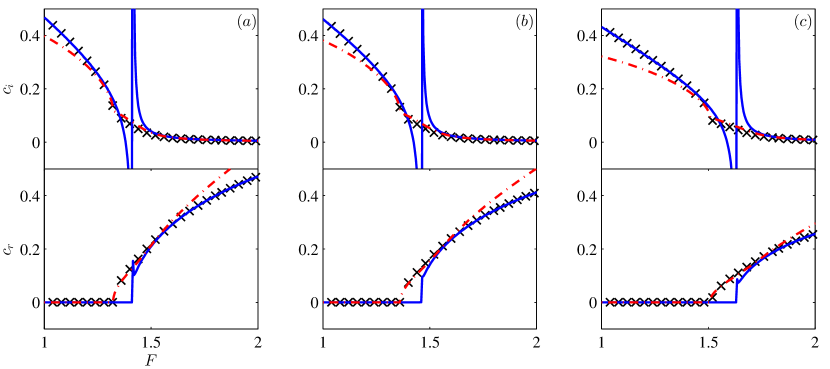
Figure 14: $c_{i}$ and $c_{r}$ versus $F$ at $\alpha=0.01$ for ($a$) $M=0$, ($b$) $M=0.25$, ($c$) $M=0.5$. The crosses are the computed results for $U(y)=\tanh y$, the solid lines are the asymptotic result $c_{\rm v}+\alpha{}c^{(1)}$ with $c^{(1)}$ given by (70), and the dot-dashed lines are the inner expansion given by the relevant solution to the cubic equation (71).

5.5.2 Jets

For a jet, $U_{\pm}=0$ and (68) simplifies to

$$0=\frac{2S_{0}^{2}}{K_{0}}+\alpha\left(\int_{-\infty}^{\infty}(S^{2}-S_{0}^{2})\,\mathrm{d}y-\frac{S_{0}^{2}}{K_{0}^{2}}\int_{-\infty}^{\infty}\left(1-\frac{S_{0}^{2}}{S^{2}}\right)\,\mathrm{d}y\right)+O(\alpha^{2}),$$ (73)

where $S_{0}^{2}=(0-c)^{2}-M^{2}$. Here, for a fixed value of $F$, we need to consider different regimes for $M$.

For $F^{2}=O(1)$, if $M^{2}=O(1)$ then $c^{(0)}$ and $c^{(1)}$ are real. To find an instability we need to consider the regime $M^{2}\sim\alpha$, which implies $c^{(0)}=0$. At the next order, we choose to balance the first two terms on the right hand side of (73), assuming that the second integral is negligible; this is confirmed by the analysis of Appendix A. Defining $E=\int^{+\infty}_{-\infty}U^{2}/2\ \textnormal{d}y$, where $U$ is assumed to decay sufficiently rapidly that $E$ is finite, we obtain

$$c\sim{}{\rm i}\sqrt{\alpha{}E-M^{2}}\qquad\textnormal{as}\qquad M^{2}\sim\alpha\to 0,\quad F^{2}=O(1).$$ (74)

The corresponding result for compressible hydrodynamics was derived by Gill & Drazin (1965), and for incompressible MHD by Gedzelman (1973).

For large $F$, the regime of interest is $M^{2}\sim\alpha$, $F^{2}\sim\alpha^{-1}$. Considering the same balance as above gives

$$c\sim{}{\rm i}\left(\frac{\alpha^{2}F^{2}E^{2}}{2}-M^{2}+\sqrt{\alpha^{2}E^{2}+\frac{\alpha^{4}F^{4}E^{4}}{4}}\right)^{1/2}\qquad\textnormal{as}\qquad F^{-2}\sim{}M^{2}\sim\alpha\to 0.$$ (75)

This result reduces to (74) in the limit of small $F$. Equations (74) and (75) are the extensions to smooth velocity profiles of equations (45) and (47), which are the dispersion relations for the even mode of the top-hat jet. It is interesting to note that the odd modes are not recovered by this analysis.

For the Bickley jet, $2E=\int^{+\infty}_{-\infty}(\textnormal{sech}^{2}y)^{2}\ \textnormal{d}y=4/3$ and (74) and (75) become

$$c\sim{\rm i}\sqrt{\frac{2}{3}\alpha-M^{2}}\qquad\textnormal{as}\qquad M^{2}\sim\alpha\to 0,\quad F^{2}=O(1),$$ (76)

and

$$c\sim{\rm i}\left(\frac{2}{9}\alpha^{2}F^{2}-M^{2}+\frac{2}{3}\sqrt{\alpha^{2}+\frac{\alpha^{4}F^{4}}{9}}\right)^{1/2}\qquad\textnormal{as}\qquad F^{-2}\sim{}M^{2}\sim\alpha\to 0.$$ (77)

In figure 15 the growth rates given by (76) and (77) are plotted against those determined numerically from equation (54); there is good agreement at small $\alpha$. The cutoff implied by (77) is also shown in figure 11$e$.

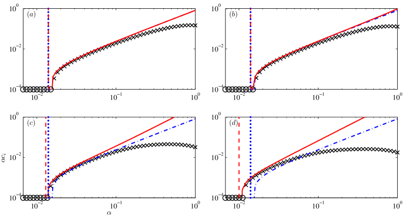
Figure 15: Comparison of the computed growth rates for the even modes (crosses) and the predicted growth rates from the asymptotic results for $U(y)=\textnormal{sech}^{2}y$, for $M=0.1$ and ($a$) $F=0$, ($b$) $F=1$, ($c$) $F=5$, ($d$) $F=10$. $\alpha\times\textrm{Im}$(76) is given by the dot-dashed line (cutoff plotted as vertical dotted line) and $\alpha\times\textrm{Im}$(77) is given by the solid line (cutoff plotted as vertical dashed line).

The above asymptotic procedure does not yield the odd modes for smooth velocity profiles; for these modes, $c_{r}$ remains $O(1)$ as $\alpha\to 0$, as can be verified numerically. The difficulty can be traced back to equation (62) since, when $M^{2}\sim\alpha$, $Z^{2}$ becomes small when $U\approx c_{r}$. The standard asymptotic procedure leading to equations (66) breaks down. Instead it is found that $c_{i}\sim\alpha^{2/3}$, a result that has been derived for the hydrodynamic case by Drazin & Howard (1962).

6 Conclusions and discussions

The SWMHD equations, introduced by Gilman (2000), are a useful model for studying MHD in thin stratified fluid layers. We have investigated the linear instability of parallel shear flows with an aligned magnetic field in planar geometry with no background rotation. The instability of hydrodynamic shear flows is a classical problem, with well known results such as Rayleigh’s inflection point criterion, Howard’s semi-circle theorem and Høiland’s growth rate bound, supplemented by extensive asymptotic and numerical results for various idealised flows. Motivated by geophysical and astrophysical considerations, previous authors have extended separately the analysis to include the influence of shallow-water dynamics and a magnetic field. Here, for the first time, we have applied this classical approach to the SWMHD system, complementing previous work on the instability of specific flow configurations in spherical geometry (Gilman & Dikpati, 2002; Dikpati et al., 2003).

We first considered the stability of arbitrary flow and field profiles, leading to the growth rate bound (9) and the semi-circle theorems (14) and (16), which, in turn, imply the stability criteria (17) – (19). More detailed investigations focused on shear layers and jets, which are known from hydrodynamical problems to be canonical flows (Drazin & Howard, 1962). For each of these we considered both discontinuous profiles, for which dispersion relations can be obtained analytically, and analogous smooth profiles, for which numerical solutions were obtained. We also took the background magnetic field to be uniform; this simple choice already leads to interesting stability characteristics. The imposed field strength is measured by a parameter $M$, whilst the stratification is measured by the Froude number $F$.

For the shear layer we considered the vortex sheet and the hyperbolic tangent velocity profile. For both profiles, a key finding is that, although increasing $M$ or $F$ in the absence of the other is seen to be stabilising, their combined effects can offset each other, resulting in a tongue of instability for arbitrarily large $F$ and $M$ approaching unity. However, the strongest instabilities are found at smaller $F$ and $M$. For the smooth shear layer, these were interpreted through the counter-propagating Rossby waves (CRWs) mechanism, which has been used to understand hydrodynamic shear instabilities (e.g., Carpenter et al., 2013). Here we show that the vorticity anomalies associated with shallow-water effects and magnetic tension oppose those for the underlying CRW mechanism. As far as we can tell, this is the first time such a dynamic argument has been invoked to explain the stabilisation of shear flow instabilities by a magnetic field. For the smooth shear layer alone, there is a weak secondary instability when $F>1$, analogous to those found in other hydrodynamic systems (Blumen et al., 1975; Balmforth, 1999). Further insight was obtained by performing a long wave asymptotic analysis for an arbitrary shear profile, extending the hydrodynamic treatment of Drazin & Howard (1962) to SWMHD. There is a primary mode of instability, yielding a dispersion relation identical to that of the vortex sheet, thus showing the widespread applicability of the vortex sheet model. For sufficiently large $F$, the long wave analysis recovers the weaker secondary mode.

For jets, we considered the top-hat velocity profile and, as its smooth counterpart, the Bickley jet. For both profiles, the modes of instability are either even or odd about the jet axis. At large $\alpha$, dynamics on the flanks of the top-hat become uncoupled, and hence the instabilities become those of the vortex sheets on the flanks. However, this behaviour does not carry over to the Bickley jet, since the even and odd modes are stabilised when $\alpha>2$ and $\alpha>1$, respectively. For small $\alpha$, the even mode is only unstable when $M<M_{c}=O(\alpha^{1/2})$. This result applies for both the top-hat profile and arbitrary smooth jets, showing the widespread applicability of the top-hat model for the even mode at small $\alpha$. For small $\alpha$, the odd mode is also only unstable for sufficiently small $M$. The growth rate $c_{i}=O(\alpha^{1/2})$ for the top-hat profile, but $c_{i}=O(\alpha^{2/3})$ for the Bickley jet, so the analogy between the top-hat and smooth velocity profiles is lost. Although we can be precise about the behaviour at large and small $\alpha$, in general either the even or odd mode may be more unstable. Finally, in addition to these two primary modes of instability, there exist multiple secondary modes of instability at large $F$, with relatively small growth rates.

Given the motivation for this study, it is important to consider the implications of our results for the solar tachocline. Adopting the tachocline radius ($\approx 0.7R_{\odot}$) as a characteristic length scale $L_{0}$ and taking $U_{0}=500\,{\rm m\,s^{-1}}$ as a characteristic velocity, as discussed in §2, the $e$-folding time for an instability is given by $\hat{t}=(\alpha c_{i})^{-1}(L_{0}/U_{0})\approx 10^{6}(\alpha c_{i})^{-1}s$. With $F\approx 0.1$, $\alpha c_{i}\approx 0.1$ over the range of $M$ anticipated for the tachocline, for both shear layers and jets (see figures 7 and 12), leading to large-scale instabilities with $\hat{t}=O(10^{7}){\rm s}$, a relevant timescale for solar dynamics.

It is hard to draw direct comparisons with previous results on SWMHD instabilities (Gilman & Dikpati, 2002; Dikpati et al., 2003; Gilman & Cally, 2007). These studies, which were focused on the tachocline, were in spherical geometry with background rotation. Furthermore, the main emphasis of the work was on the destabilisation of hydrodynamically stable velocity profiles by non-uniform toroidal fields.

Having investigated the quite complicated behaviour that results from our idealised model, there are, within the present geometry, several natural extensions of our study. The inclusion of rotation could be considered; even in the hydrodynamic case this modifies the nature of the instabilities. Non-uniform magnetic fields open up the possibility of destabilising hydrodynamically stable velocity profiles, as in Gilman & Dikpati (2002) and Dikpati et al. (2003). The nonlinear evolution of the instability and the associated changes in the mean flow are clearly of interest; some preliminary results are given in Mak (2013).

This work was supported by the STFC doctoral training grant ST/F006934/1. JM thanks Eyal Heifetz for helpful discussions.

Appendix A Consistency checks for the long-wavelength jet analysis

The aim of this appendix is to show that

$$\frac{c^{2}-M^{2}}{1-F^{2}(c^{2}-M^{2})}\int^{+\infty}_{-\infty}\left(1-\frac{c^{2}-M^{2}}{(U-c)^{2}-M^{2}}\right)\ \textnormal{d}y$$ (78)

is $O\left(\alpha\log(\alpha)\right)$, and hence that the asymptotic analysis of § 5.5.2 is consistent.

Following Drazin & Howard (1962), we assume that $|U|\leq{}A\mathrm{e}^{-a|y|}$, which is satisfied for the Bickley jet. They make the additional assumption that $c$ is ‘almost pure imaginary’; here we adopt the modified assumption that

$$\frac{|c|^{2}+M^{2}}{c_{i}^{2}}\leq{}N=O(1),$$ (79)

which is supported by both our numerical and asymptotic results.

Consider first the case of $F=0$ for which (78) is given by

$$I=(c^{2}-M^{2})\int^{\infty}_{-\infty}\left(1-\frac{c^{2}-M^{2}}{(U-c)^{2}-M^{2}}\right)\ \textnormal{d}y.$$ (80)

For $y>0$, we split the range of integration into $(0,\lambda)$ and $(\lambda,\infty)$, where

$$\lambda=\log\left(\frac{A}{c}\right)^{1/a}=O\left(\log(\alpha)\right),$$ (81)

since $c^{2}=O(\alpha)$. Then

$$(c^{2}-M^{2})\int^{\lambda}_{0}(\cdots)\ \textnormal{d}y\leq|c^{2}-M^{2}|\int^{\lambda}_{0}\left(1+\frac{|c|^{2}+M^{2}}{c_{i}^{2}}\right)\ \textnormal{d}y\\ \leq|c^{2}-M^{2}|\lambda\left(1+N\right)=O(\alpha\log\alpha),$$ (82)

where we have used the usual integral inequalities, the inequality $|(U-c)^{2}-M^{2}|\geq{}c_{i}^{2}$, the assumption that $M^{2}=O(\alpha)$, and the derived result (74) that $c=O(\alpha^{1/2})$.

Similarly,

$$(c^{2}-M^{2})\int^{\infty}_{\lambda}(\cdots)\ \textnormal{d}y=(c^{2}-M^{2})\int^{\infty}_{\lambda}\left(\frac{U^{2}-2Uc}{(U-c)^{2}-M^{2}}\right){\rm d}y\\ \leq\frac{|c^{2}-M^{2}|}{c_{i}^{2}}\int^{\infty}_{\lambda}\left(U^{2}+2|U||c|\right)\textnormal{d}y\leq{}N\left(\dfrac{A^{2}\mathrm{e}^{-2a\lambda}}{2a}+\dfrac{2A|c|\mathrm{e}^{-a\lambda}}{a}\right)=O(\alpha).$$

The dominant contribution is from (82), and hence $I=O(\alpha\log\alpha)$.

When $F$ is non-zero, the only difference is in the pre-factor to the integral (78). However, with $c$ from either (76) or (77) the pre-factor is $O(1)$ and we may conclude that $I=O(\alpha\log\alpha)$.

References

- Baines & Mitsudera (1994) Baines, P. G. & Mitsudera, H. 1994 On the mechanism of shear instabilities. J. Fluid Mech. 276, 327–342.
- Balmforth (1999) Balmforth, N. J. 1999 Shear instability in shallow water. J. Fluid Mech. 387, 97–127.
- Bazdenkov & Pogutse (1983) Bazdenkov, S. V. & Pogutse, O. P. 1983 Supersonic stabilization of a tangential shear in a thin atmosphere. JETP Lett. 37, 375–377.
- Blumen et al. (1975) Blumen, W., Drazin, P. G. & Billings, D. F. 1975 Shear layer instability of an inviscid compressible fluid. Part 2. J. Fluid Mech. 71, 305–316.
- Bretherton (1966) Bretherton, F. P. 1966 Baroclinic instability and the short wavelength cut-off in terms of potential vorticity. Q. J. Roy. Met. Soc. 92, 335–345.
- Cally (2003) Cally, P. S. 2003 Three-dimensional magneto-shear instabilities in the solar tachocline. Mon. Not. R. Astron. Soc. 339, 957–972.
- Carpenter et al. (2013) Carpenter, J. R., Tedford, E. W., Heifetz, E. & Lawrence, G. A. 2013 Instability in stratified shear flow: Review of a physical interpretation based on interacting waves. Appl. Mech. Rev. 64, 061001.
- Collings & Grimshaw (1980) Collings, I. L. & Grimshaw, R. H. J. 1980 The effect of topography on the stability of a barotropic coastal current. Dyn. Atmos. Ocean. 5, 83–106.
- De Sterck (2001) De Sterck, H. 2001 Hyperbolic theory of the “shallow water” magnetohydrodynamics equations. Phys. Plasmas 8, 3293–3304.
- Dellar (2002) Dellar, P. J. 2002 Hamiltonian and symmetric hyperbolic structures of shallow water magnetohydrodynamics. Phys. Plasmas 9, 1130–1136.
- Dikpati & Gilman (2001) Dikpati, M. & Gilman, P. A. 2001 Analysis of hydrodynamic stability of solar tachocline latitudinal differential rotation using a shallow-water model. Astrophys. J. 551, 536–564.
- Dikpati et al. (2003) Dikpati, M., Gilman, P. A. & Rempel, M. 2003 Stability analysis of tachocline latitudinal differential rotation and coexisting toroidal band using a shallow-water model. Astrophys. J. 596, 680–697.
- Drazin & Howard (1962) Drazin, P. G. & Howard, L. N. 1962 The instability to long waves of unbounded parallel inviscid flow. J. Fluid Mech. 14, 257–283.
- Drazin & Howard (1966) Drazin, P. G. & Howard, L. N. 1966 Hydrodynamic stability of parallel flow of inviscid fluid. Advan. Appl. Mech. 9, 1–89.
- Drazin & Reid (1981) Drazin, P. G. & Reid, W. H. 1981 Hydrodynamic Stability, 2nd edn. Cambridge University Press.
- Gedzelman (1973) Gedzelman, S. D. 1973 Hydromagnetic stability of parallel flow of an ideal heterogeneous fluid. J. Fluid Mech. 58, 777–794.
- Gill (1965) Gill, A. E. 1965 Instabilities of “top-hat” jets and wakes in compressible fluids. Phys. Fluids 8, 1428–1430.
- Gill (1982) Gill, A. E. 1982 Atmosphere-Ocean Dynamics. Academic Press.
- Gill & Drazin (1965) Gill, A. E. & Drazin, P. G. 1965 Note on instability of compressible jets and wakes to long-wave disturbance. J. Fluid Mech. 22, 415–415.
- Gilman (2000) Gilman, P. A. 2000 Magnetohydrodynamic “shallow water” equations for the solar tachocline. Astrophys. J. 544, L79–L82.
- Gilman & Cally (2007) Gilman, P. A. & Cally, P. S. 2007 Global MHD instabilities of the tachocline. In The Solar Tachocline (ed. D. W. Hughes, R. Rosner & N. O. Weiss). Cambridge University Press.
- Gilman & Dikpati (2002) Gilman, P. A. & Dikpati, M. 2002 Analysis of instability of latitudinal differential rotation and toroidal field in the solar tachocline using a magnetohydrodynamic shallow-water model. I. Instability for broad toroidal field profiles. Astrophys. J. 576, 1031–1047.
- Gough (2007) Gough, D. O. 2007 An introduction to the solar tachocline. In The Solar Tachocline (ed. D. W. Hughes, R. Rosner & N. O. Weiss). Cambridge University Press.
- Harnik & Heifetz (2007) Harnik, N. & Heifetz, E. 2007 Relating overreflection and wave geometry to the counter-propagating Rossby wave perspective: Toward a deeper mechanistic understanding of shear instability. J. Atmos. Sci. 64, 2238–2261.
- Hayashi & Young (1987) Hayashi, Y.-Y. & Young, W. R. 1987 Stable and unstable shear modes of rotating parallel flows in shallow water. J. Fluid Mech. 184, 477–504.
- Heifetz et al. (2004) Heifetz, E., Bishop, C. H., Hoskins, B. J. & Methven, J. 2004 The counter-propagating Rossby-wave perspective on baroclinic instability. I: Mathematical basis. Q. J. Roy. Met. Soc. 130, 211–231.
- Heng & Spitkovsky (2009) Heng, K. & Spitkovsky, A. 2009 Magnetohydrodynamic shallow water waves: Linear analysis. Astrophys. J. 703, 1819–1831.
- Høiland (1953) Høiland, E. 1953 On two-dimensional perturbation of linear flow. Geofys. Publ. 18, 333–342.
- Hoskins et al. (1985) Hoskins, B. J., McIntyre, M. E. & Robertson, A. W. 1985 On the use and significance of isentropic potential vorticity maps. Q. J. Roy. Met. Soc. 111, 877–946.
- Howard (1961) Howard, L. N. 1961 Note on a paper of John W. Miles. J. Fluid Mech. 10, 509–512.
- Howard (1963) Howard, L. N. 1963 Neutral curves and stability boundaries in stratified flow. J. Fluid Mech. 16, 333–342.
- Hughes et al. (2007) Hughes, D. W., Rosner, R. & Weiss, N. O. 2007 The Solar Tachocline. Cambridge University Press.
- Hughes & Tobias (2001) Hughes, D. W. & Tobias, S. M. 2001 On the instability of magnetohydrodynamic shear flows. Proc. R. Soc. Lond. A 457, 1365–1384.
- Lipps (1962) Lipps, F. B. 1962 The barotropic stability of the mean winds in the atmosphere. J. Fluid Mech. 12, 397–407.
- Mak (2013) Mak, J. 2013 Shear instabilities in shallow-water magnetohydrodynamics. PhD thesis, University of Leeds.
- Michael (1955) Michael, D. H. 1955 Stability of a combined current and vortex sheet in a perfectly conducting fluid. Proc. Camb. Phil. Soc. 51, 528–532.
- Michalke (1964) Michalke, A. 1964 On the inviscid instability of the hyperbolic-tangent velocity profile. J. Fluid Mech. 19, 543–556.
- Miles (1958) Miles, J. W. 1958 On the disturbed motion of a vortex sheet. J. Fluid Mech. 4, 538–552.
- Miura & Pritchett (1982) Miura, A. & Pritchett, P. L. 1982 Nonlocal stability analysis of the MHD Kelvin-Helmholtz instability in a compressible plasma. J. Geophys. Res. 87, 7431–7444.
- Pedlosky (1964) Pedlosky, J. 1964 The stability of currents in the atmosphere and the ocean: Part I. J. Atmos. Sci. 21, 201–219.
- Rayleigh (1878) Rayleigh, Lord 1878 On the instability of jets. Proc. London Math. Soc. 10, 4–12.
- Ripa (1983) Ripa, P. 1983 General stability conditions for zonal flows in a one-layer model on the -plane or the sphere. J. Fluid Mech. 126, 463–489.
- Satomura (1981) Satomura, T. 1981 An investigation of shear instability in a shallow water. J. Met. Soc. Japan 59, 148–170.
- Schecter et al. (2001) Schecter, D. A., Boyd, J. F. & Gilman, P. A. 2001 “Shallow-water” magnetohydrodynamic waves in the solar tachocline. Astrophys. J. 551, L185–L188.
- Shivamoggi & Debnath (1987) Shivamoggi, B. K. & Debnath, L. 1987 Stability of magnetohydrodynamic stratified shear flows. Acta Mech. 68, 33–42.
- Sutherland & Peltier (1992) Sutherland, B. R. & Peltier, W. R. 1992 The stability of stratified jets. Geophys. Astrophys. Fluid Dyn. 66, 101–131.
- Takehiro & Hayashi (1992) Takehiro, S. I. & Hayashi, Y. Y. 1992 Over-reflection and shear instability in a shallow-water model. J. Fluid Mech. 236, 259–279.
- Vallis (2006) Vallis, G. K. 2006 Atmospheric and Oceanic Fluid Dynamics. Cambridge University Press.
- Zaqarashivili et al. (2008) Zaqarashivili, T. V., Oliver, R., Ballester, J. L. & Shergelashvili, B. M. 2008 Rossby waves in “shallow water” magnetohydrodynamics. Astron. Astrophys. 470, 815–820.