1

Spontaneous Motion on Two-dimensional Continuous Attractors

C. C. Alan Fung¹ and S. Amari^2
1Department of Physics, The Hong Kong University of Science and Technology, Clear Water Bay, Hong Kong, China.
²Laboratory for Mathematical Neuroscience, RIKEN Brain Science Institute, Saitama, 351-0198, Japan.

Keywords: Continuous Attractor Neural Networks, Short-term Synaptic Depression, Spike Frequency Adaptation

Abstract

Attractor models are simplified models used to describe the dynamics of firing rate profiles of a pool of neurons. The firing rate profile, or the neuronal activity, is thought to carry information. Continuous attractor neural networks (CANNs) describe the neural processing of continuous information such as object position, object orientation and direction of object motion. Recently, it was found that, in one-dimensional CANNs, short-term synaptic depression can destabilize bump-shaped neuronal attractor activity profiles. In this paper, we study two-dimensional CANNs with short-term synaptic depression and with spike frequency adaptation. We found that the dynamics of CANNs with short-term synaptic depression and CANNs with spike frequency adaptation are qualitatively similar. We also found that in both kinds of CANNs the perturbative approach can be used to predict phase diagrams, dynamical variables and speed of spontaneous motion.

1 Introduction

Neurons communicate with each other through the neurotransmitter diffusion initiated by action potentials, or spikes, and the activity of one neuron can excite or inhibit the activity of another neurons. The firing rates of spike trains are thought to carry information and correlations between the firing rates of neurons depend on the strength of the couplings between those neurons. With some specific settings of couplings (e.g., Mexican-hat couplings (Amari, 1977; Ben-Yishai et al., 1995)) networks of neurons can support a continuous family of local neuronal activity profiles on a field, which can be used to represent continuous information, such as object position, object orientation and direction of object motion.

Local neuronal activities associated with continuous information are observed in various brain regions. Typical examples of cells showing such activity are head-direction cells (Taube et al., 1990; Blair & Sharp, 1995; Zhang, 1996; Taube & Muller, 1998), place cells (O’Keefe & Dostrovsky, 1971; O’Keefe, 1976; O’Keefe & Burgess, 1996; Samsonovich & McNaughton, 1997) and moving-direction cells (Maunsell & van Essen, 1983; Treue et al., 2000). These cells have Gaussian-like tuning curves as functions of stimulus. Among the numerous models proposed to describe behaviors of these systems are continuous attractor neural networks (CANNs), and a recent study of persistent activity in monkey prefrontal cortices has provided evidence of continuous attractors in the central nervous system. (Wimmer et al., 2014). Persistent neuronal activity in monkeys’ prefrontal cortices was discovered during delayed-response tasks (Funahashi et al., 1993). The study by Wimmer et al. (2014) confirmed that pairwise neuronal correlation predicted by theories can be observed in the brain region they investigated (Ben-Yishai et al., 1995; Pouget et al., 1998; Wu et al., 2008).

A one-dimensional (1D) CANN can support a family of Gaussian-like neuronal activity profiles. They are attractors of the network. As shown in Figure 1(a), attractors have the same shapes and are centered at positions corresponding to different preferred stimuli. These Gaussian-like profiles can shift smoothly along the space of attractors. Families of attractor profiles in two-dimensional (2D) CANNs are similar: each attractor profile is a Gaussian-like profile and centered at a particular position in the 2D field (Figure 1(b)). The dynamics of a network state profile to track a stimulus is widely studied in the literature (Ben-Yishai et al., 1995; Samsonovich & McNaughton, 1997; Wu et al., 2008; Fung et al., 2010). If couplings between neurons are static over time (quenched), the steady state of neuronal activity profiles will be static because of the homogeneity and translational invariance of CANNs. If they depend on the firing histories of presynaptic neurons, however, the dynamics of CANNs can be different.

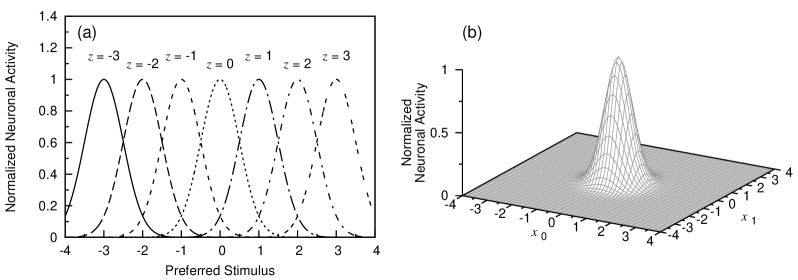
Figure 1: Examples of attractor states of continuous attractor neural networks (CANNs) in (a) a 1D field and (b) a 2D field. In (a), profiles are centered at location $z$, the location they are representing. In (b), $x_{0}$ is the first coordinate of the preferred stimulus and $x_{1}$ is the second coordinate of the preferred stimulus.

Tsodyks & Markram (1997) proposed a model in which the synaptic efficacies between neurons depend on the amount of available neurotransmitters in the presynaptic neurons and this amount depends on the firing history of the presynaptic neuron (Tsodyks & Markram, 1997; Tsodyks et al., 1998). This kind of reduction in synaptic efficacies, due to past presynaptic neuronal activity, is called short-term synaptic depression (STD). There are reports that short-term synaptic depression can exhibit rich dynamics in CANNs (York & van Rossum, 2009; Fung et al., 2012a). Fung et al. (2012a) reported that in 1D CANNs, short-term synaptic depression can destabilize attractor profiles. Within a broad range of strengths of divisive global inhibition, if we increase the degree of STD to a moderate range, static activity profiles will be translationally destabilized. After some translational perturbations, a bump-shaped profile can move spontaneously along the attractor space. In these scenarios, both bump-shaped static states and moving states can coexist. If we further increase the degree of STD, no static profile can be found. If the degree of STD is too large, the steady state of the system can only be a trivial solution. Similar behavior is reported by York & van Rossum (2009) with a different model. We can see that the instability induced by STD can reshape the intrinsic dynamics of the system, even when no stimulus is presented.

Network response in a CANN with static couplings is always lagging behind a continuously moving stimulus. However, with short-term synaptic depression, due to the translational instability, the underlying dynamics of the network can make the response to over-take the actual stimulus. Fung et al. (2012b) suggested that this behavior can be used to implement a delay compensation mechanism. Short-term synaptic depression can also induce global (Leobel & Tsodyks, 2002) and local (Fung et al., 2013; Wang et al., Unpublished) periodic excitements of neuronal activity profiles. These periodic excitements can enhance information processing in the brain. Fung et al. (2013) recently proposed that periodic excitement driven by the intrinsic dynamics can improve the resolution of CANNs. Kilpatrick (2013) also proposed that the neuronal activity pattern may shift between one stimulus and another. These theories suggested that STD may enhance the capability of CANNs.

Studies on CANNs with short-term synaptic depression are mainly on 1D networks. In this paper, we discuss the intrinsic dynamics of bump-shaped solutions of two-dimensional CANNs with short-term synaptic depression. Other 2D models possess rich dynamical behaviors such as spiral waves (Kilpatrick & Bressloff, 2010a), breathing pulses (Kilpatrick & Bressloff, 2010a) and collisions of two bump-shaped profiles (Lu et al., 2011). Here, we focus on the spontaneous motion of a single bump-shaped profile, and analyze its stability. We have also studied the influence of STD on the sizes of bump-shaped profiles and on their changes in shape.

We study not only CANNs with STD, but also CANNs with spike frequency adaptation. Spike frequency adaptation (SFA) is a dynamical feature commonly observed in neurons. Neurons are suppressed after prolonged firing. SFA can be generated by a number of mechanisms (Brown & Adams, 1980; Madison & Nicoll, 1984; Fleidervish et al., 1996; Benda & Herz, 2003). It can also destabilize the amplitudes and positions of static bumps. SFA-induced destabilization of bump-shaped states in CANNs are reported in the literature (e.g., Kilpatrick & Bressloff, 2010b). What we find in our study on CANNs with SFA is similar to what we found in the case with STD. SFA first destabilizes the translational mode and then the amplitudal mode. There is also a parameter region such that both spontaneous-moving-bump solutions and static-bump solutions can coexist.

In this paper, in each case, CANNs with STD and CANNs with SFA, we first introduce the model we used to study the problem and then analyze each scenario using the perturbative method proposed by Fung et al. (2010). These sections are followed by a section discussing the comparison between theoretical and simulation results and discussing the limitations of the perturbative method.

2 The Model

In this work we consider a 2D neural field, where neurons are located on a 2D field with positional coordinates $\mathbf{x}=\left(x_{0},x_{1}\right)$. $\mathbf{x}$ can be interpreted as the preferred stimulus of the neuron sitting at that point in the 2D field. The state of a neural field is specified by the average membrane potential $u\left(\mathbf{x},t\right)$ of neurons at $\mathbf{x}$ at time $t$. The neuronal activity of a neuron at $\mathbf{x}$ is given by a nonlinear function of $u\left(\mathbf{x},t\right)$:

$$r\left(\mathbf{x},t\right)=\frac{u\left(\mathbf{x},t\right)^{2}}{B\left(t\right)}\Theta\left[u\left(\mathbf{x},t\right)\right],$$ (1)

where $\Theta$ is the Heaviside step function and $B\left(t\right)$ is the divisive global inhibition. The neuronal activity is related to the average firing rate of the neuron. The evolution of the global inhibition is given by

$$\tau_{B}\frac{dB\left(t\right)}{dt}=-B\left(t\right)+1+\rho k\int d\mathbf{x}^{\prime}u\left(\mathbf{x}^{\prime},t\right)^{2}\Theta\left[u\left(\mathbf{x}^{\prime},t\right)\right],$$ (2)

where $k$ is the parameter controlling the strength of the divisive global inhibition and $\rho$ is the density of neurons over the field. Here, $B\left(t\right)$ is driven by $u\left(\mathbf{x},t\right)^{2}$. This choice of driving term can simplify our calculations. As we will describe in the following, $u\left(\mathbf{x},t\right)$ is a weighted sum of $r\left(\mathbf{x},t\right)$. So $B\left(t\right)$ effectively depends on $r\left(\mathbf{x},t\right)$. Also, at the steady state, the magnitude of $u\left(\mathbf{x},t\right)$ is directly proportional to that of $r\left(\mathbf{x},t\right)$.

In the network, neurons are connected by excitatory couplings given by

$$J\left(\left|\mathbf{x}-\mathbf{x^{\prime}}\right|\right)=\frac{J_{0}}{2\pi a^{2}}\exp\left(-\frac{\left|\mathbf{x}-\mathbf{x^{\prime}}\right|^{2}}{2a^{2}}\right),$$ (3)

where $\left|~{}\cdot~{}\right|$ is the norm of the argument. $a$ is the radius of effective excitatory connections and $J_{0}$ is the intensity of average coupling over the field. The dynamics of $u\left(x,t\right)$ is governed by

$$\tau_{s}\frac{\partial u\left(\mathbf{x},t\right)}{\partial t}= -u\left(\mathbf{x},t\right)+\rho\int d\mathbf{x^{\prime}}J\left(\left|\mathbf{x}-\mathbf{x^{\prime}}\right|\right)p\left(\mathbf{x^{\prime}},t\right)r\left(\mathbf{x^{\prime}},t\right)$$

$$-v\left(\mathbf{x},t\right)+I^{\text{ext}}\left(\mathbf{x},t\right).$$ (4)

$I^{\text{ext}}\left(\mathbf{x},t\right)$ is the external stimulus, $p\left(\mathbf{x},t\right)$ is the portion of available neurotransmitters of the presynaptic neuron and $v\left(\mathbf{x},t\right)$ is the dynamical variable corresponding to SFA. Since in this work, we are studying intrinsic dynamics in the network, $I^{\rm ext}\left(\mathbf{x},t\right)$ is set to zero throughout the paper.

The portion of available neurotransmitters of the presynaptic neuron at $\mathbf{x}$, $p\left(\mathbf{x},t\right)$, evolves as

$$\tau_{d}\frac{\partial p\left(\mathbf{x},t\right)}{\partial t}=-p\left(\mathbf{x},t\right)+1-\tau_{d}\beta p\left(\mathbf{x},t\right)r\left(\mathbf{x},t\right).$$ (5)

The first term on the right-hand side of this equation is the relaxation of $p\left(\mathbf{x},t\right)$ with time constant $\tau_{d}$. The last term is the consumption rate of neurotransmitters. $\beta$ is a parameter proportional to the neurotransmitter consumption due to each spikes. This parameter controls the strength of STD. On the other hand, the dynamics of $v\left(\mathbf{x},t\right)$ is given by

$$\tau_{i}\frac{dv}{dt}\left(\mathbf{x},t\right)=-v\left(\mathbf{x},t\right)+\gamma f\left[u\left(\mathbf{x},t\right)\right].$$ (6)

$\tau_{i}$ is the timescale of SFA. $\gamma$ is the degree of SFA. $f$ is the dependence of SFA variables on average membrane potential, which is a non-decreasing function. For simplicity, we have chosen

$$f\left(u\right)=u\Theta\left(u\right).$$ (7)

This choice is convenient for our analytic purpose and should not affect the main conclusion qualitatively as long as the adaptation increases with the average membrane potential, $u\left(\mathbf{x},t\right)$, which is correlated with the average neuronal activity.

In the present study, we analyze CANNs with STD and CANNs with SFA separately. For the case of CANNs with STD, we set $\gamma=0$. For CANNs with SFA, we set $\beta=0$.

3 CANNs with STD

3.1 Stationary Solution

In this case, we set $\gamma=0$ and $I^{\rm ext}\left(\mathbf{x},t\right)=0$ to suppress SFA at the moment. For $\beta=0$, $p\left(\mathbf{x},t\right)=1$, two types of non-zero fixed point solutions to Eq. (4) exist when $0<k<k_{c}\equiv\rho J_{0}^{2}/\left(32\pi a\right)$:

$$u\left(\mathbf{x}\right)=u_{00}\exp\left(-\frac{\left|\mathbf{x}-\mathbf{z}\right|^{2}}{4a^{2}}\right),$$ (8)

where $\rho J_{0}u_{00}=4(1\pm\sqrt{1-k/k_{c}})/(k/k_{c})$ and $\mathbf{z}$ is an arbitrary location in the field representing the center of local excitation. It is expected that the fixed point solution with the larger amplitude is stable and the other is unstable. For $\tau_{B}=0$, consider

$$u\left(\mathbf{x},t\right)=\left[u_{00}+\delta u_{00}\left(t\right)\right]\exp\left(-\frac{\left|\mathbf{x}-\mathbf{z}\right|^{2}}{4a^{2}}\right),$$ (9)

where $\delta u_{00}\left(t\right)$ is the deviation of the profile from the fixed point solution. Then the differential equation of the deviation is

$$\tau_{s}\frac{d\delta u_{00}\left(t\right)}{dt}=\mp\sqrt{1-\frac{k}{k_{c}}}\delta u_{00}\left(t\right).$$ (10)

Therefore the smaller fixed point solutions are unstable, while the larger fixed point solutions have stable amplitudes. For non-zero $\tau_{B}$, we have to consider the dynamics of $B(t)$. Let $B(t)=B_{0}+\delta B(t)$, where $B_{0}=1+\tfrac{1}{16}\left(k/k_{c}\right)\left(\rho J_{0}u_{00}\right)^{2}$. The dynamics of the deviation from the fixed point solution is given by

$$\tau_{s}\frac{d}{dt}\left(\begin{array}[]{c}\rho J_{0}\delta u_{00}\left(t\right)\\ \delta B\left(t\right)\end{array}\right)=\left(\begin{array}[]{cc}1&-2\\ \frac{1}{2}\frac{\tau_{s}}{\tau_{B}}(1\pm\sqrt{1-\frac{k}{k_{c}}})&-\frac{\tau_{s}}{\tau_{B}}\end{array}\right)\left(\begin{array}[]{c}\rho J_{0}\delta u_{00}\left(t\right)\\ \delta B\left(t\right)\end{array}\right).$$ (11)

Since the trace of the $2\times 2$ matrix in Eq. (11) is negative for $\tau_{B}<\tau_{s}$ and the sign of the determinant is independent of $\tau_{s}/\tau_{B}$, the solution with the larger $u_{00}$ is stable against perturbations in amplitude, while the solution with the smaller amplitude is unstable. The solution of $u_{00}$ as a function of $k/k_{c}$ is shown in Figure 2.

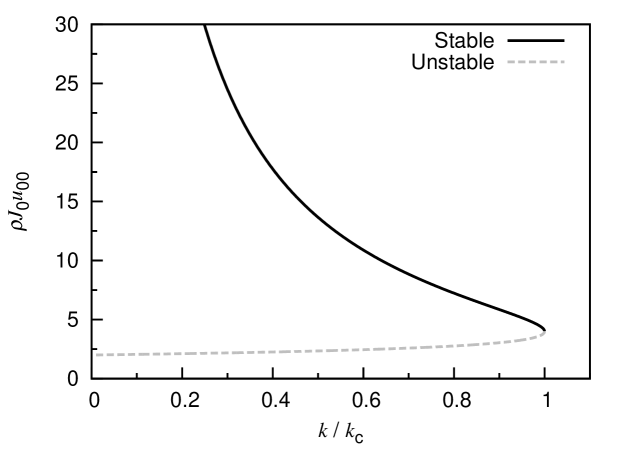
Figure 2: Solution of $\rho J_{0}u_{00}$ as a function of $k/k_{c}$. For each $k/k_{c}$ less than 1, the larger solution of $\rho J_{0}u_{00}$ is stable and the smaller solution is unstable.

For $\beta>0$ and $I^{\text{ext}}\left(\mathbf{x},t\right)=0$, we approximate the attractor profiles of $u\left(\mathbf{x},t\right)$ and $1-p(\mathbf{x},t)$ by non-moving Gaussian distributions

$$u\left(\mathbf{x},t\right)= ~{}u_{00}\left(t\right)\exp\left(-\frac{\left|\mathbf{x}\right|^{2}}{4a^{2}}\right),$$ (12)

$$1-p\left(\mathbf{x},t\right)= ~{}p_{00}\left(t\right)\exp\left(-\frac{\left|\mathbf{x}\right|^{2}}{2a^{2}}\right).$$ (13)

Here, without loss of generality, we consider the case with $\mathbf{z}=\mathbf{0}$. They are not the exact solutions of Eqs. (2), (4) and (5). In this ansatz, $u\left(\mathbf{x},t\right)$ is assumed to have the same shape as that in the $\beta=0$ case. The width of $1-p\left(\mathbf{x},t\right)$ is different from $u\left(\mathbf{x},t\right)$ because the shape of $1-p\left(\mathbf{x},t\right)$ is similar to $u\left(\mathbf{x},t\right)^{2}$ at the small $\beta$ limit. The differential equations governing $u_{00}\left(t\right)$ and $p_{00}\left(t\right)$ can be obtained by projecting Eq. (4) onto $\exp[-\left|\mathbf{x}\right|^{2}/(4a^{2})]$ and projecting Eq. (5) onto $\exp[-\left|\mathbf{x}\right|^{2}/(2a^{2})]$.

As in the study by Fung et al. (2012a), $u\left(\mathbf{x},t\right)$ can be replaced by rescaled variables $\widetilde{u}\left(\mathbf{x},t\right)\equiv\rho J_{0}u\left(\mathbf{x},t\right)$ because $u_{00}\left(t\right)$ has a dimension $1/(\rho J_{0})$. $\widetilde{u}_{00}\left(t\right)\equiv\rho J_{0}u_{00}\left(t\right)$. And $k$ and $\beta$ can be rescaled by $\widetilde{k}\equiv k/k_{c}$ and $\widetilde{\beta}\equiv\tau_{d}\beta/(\rho^{2}J_{0}^{2})$.

Figure 3: Parameter regions of existence of static profiles of $u(\mathbf{x},t)$. Dashed curves: parabolas given by Eq. (17) for different $\widetilde{\beta}B$’s. Solid line: boundary separating parameter regions of static profiles of $u(\mathbf{x},t)$ and silent phase.

With these rescaled variables, the differential equations of $\widetilde{u}_{00}\left(t\right)$, $p_{00}\left(t\right)$ and $B\left(t\right)$ are

$$\tau_{s}\frac{d\widetilde{u}_{00}}{dt}\left(t\right)= ~{}-\widetilde{u}_{00}\left(t\right)+\frac{1}{2}\frac{1}{B\left(t\right)}\widetilde{u}_{00}\left(t\right)^{2}\left[1-\frac{4}{7}p_{00}\left(t\right)\right],$$ (14)

$$\tau_{d}\frac{dp_{00}}{dt}\left(t\right)= ~{}-p_{00}\left(t\right)+\frac{1}{B\left(t\right)}\widetilde{\beta}\widetilde{u}_{00}\left(t\right)^{2}\left[1-\frac{2}{3}p_{00}\left(t\right)\right],$$ (15)

$$\tau_{B}\frac{dB}{dt}\left(t\right)= ~{}-B\left(t\right)+1+\frac{1}{16}\widetilde{k}\widetilde{u}_{00}\left(t\right)^{2}.$$ (16)

As we study the steady state behavior of the network, we need to solve for the fixed point solution first. For the first two differential equations, we may let $\widetilde{\beta}B$ be given. Then we can solve $\widetilde{u}_{00}/B$ and $p_{00}$. For a given $\widetilde{\beta}B$, $\widetilde{k}$ and $\widetilde{\beta}$ are related by

$$\widetilde{k}=\frac{16}{\left(\frac{\widetilde{u}_{00}}{B}\right)^{2}}\left[-\frac{1}{\left(B\widetilde{\beta}\right)^{2}}\widetilde{\beta}^{2}+\frac{1}{B\widetilde{\beta}}\widetilde{\beta}\right].$$ (17)

The parabolas given by this equation for different $\widetilde{\beta}B$s are plotted as dashed lines in Figure 3, where we see that the static fixed point solution exists only when

$$\begin{cases}\widetilde{\beta}\leq\frac{3}{16}\widetilde{k}\frac{1-\sqrt{\widetilde{k}}}{\sqrt{\widetilde{k}}-\frac{1}{7}}&\text{, if }\frac{9}{49}\leq\widetilde{k}\leq 1\\ \widetilde{\beta}\leq\frac{9}{56}\left(\frac{3}{7}-\sqrt{\frac{9}{49}-\widetilde{k}}\right)&\text{, if }0\leq\widetilde{k}\leq\frac{9}{49}\end{cases}.$$ (18)

By considering the stability of fixed point solutions, we obtain the solid line in Figure 3 (also the dotted line in Figure 4). This curve maps the parameter region for the existence of static profiles of $u(\mathbf{x},t)$. The methodology for studying stability of fixed point solutions can be found in Appendix A.

3.1 Translational Instability

We have simplified Eqs. (2), (4) and (5) by introducing the approximation given by Eqs. (12) and (13). This simplification, however, is useful for studying only the amplitudal stability of a bump-shaped solution. For the translational stability, we need to consider the stability of the static solution against asymmetric distortions. Displacing originally aligned $u\left(\mathbf{x},t\right)$ and $p\left(\mathbf{x},t\right)$ profiles of a static solution is a reasonable test, as the dip of $p\left(\mathbf{x},t\right)$ is generated by activities of neurons. If the solution is moving, the dip of $p\left(\mathbf{x},t\right)$ is always lagging behind. As a result, the asymmetric component of $p\left(\mathbf{x},t\right)$ with respect to the center of mass of $u\left(\mathbf{x},t\right)$ becomes non-zero. In the calculation, we may drop asymmetric components of $u\left(\mathbf{x},t\right)$ for the moment, as we can always choose a frame such that the major asymmetric mode is zero.

Let us assume

$$u\left(\mathbf{x},t\right)= ~{}u_{00}\left(t\right)\exp\left(-\frac{\left|\mathbf{x}\right|^{2}}{4a^{2}}\right),$$ (19)

$$p\left(\mathbf{x},t\right)= ~{}p_{00}\left(t\right)\exp\left(-\frac{\left|\mathbf{x}\right|^{2}}{2a^{2}}\right)+p_{10}\left(t\right)\frac{x_{0}}{a}\exp\left(-\frac{\left|\mathbf{x}\right|^{2}}{2a^{2}}\right).$$ (20)

Due to the symmetry of the preferred stimulus space, here we consider only the distortion along the $x_{0}$-direction. By substituting these two assumptions into Eqs. (2), (4) and (5), we can study the stability of static solutions against asymmetric distortions. With assumptions Eqs. (19) and (20), we can derive the stability matrix by calculating the Jacobian matrix at the fixed point solution. Then the dynamics of distortions of $\widetilde{u}_{00}\left(t\right)$, $p_{00}\left(t\right)$, $p_{10}\left(t\right)$ and $B\left(t\right)$ around the static fixed point solution is given by

$$\tau_{s}\frac{d}{dt}\left(\begin{array}[]{c}\delta\widetilde{u}_{00}\left(t\right)\\ \delta p_{00}\left(t\right)\\ \delta B\left(t\right)\\ \delta p_{10}\left(t\right)\end{array}\right)=\left(\begin{array}[]{cc}\mathscr{A}_{\rm STD}&0\\ 0&M\end{array}\right)\left(\begin{array}[]{c}\delta\widetilde{u}_{00}\left(t\right)\\ \delta p_{00}\left(t\right)\\ \delta B\left(t\right)\\ \delta p_{10}\left(t\right)\end{array}\right),$$ (21)

where the $3\times 3$ matrix $\mathscr{A}_{\rm STD}$ is provided in Appendix A. $\mathscr{A}_{\rm STD}$ determines the amplitudal stability of the solution, while $M$ determines translational stability, which is given by

$$M=\frac{1}{\tau_{d}}\left(-1+\frac{\widetilde{\beta}}{B}\frac{4}{9}\widetilde{u}_{00}^{2}+\frac{\tau_{d}}{\tau_{s}}\frac{1}{B}\frac{8}{49}\widetilde{u}_{00}\widetilde{p}_{00}\right).$$ (22)

If $M>0$, the static solution of two-dimensional CANNs with short-term synaptic depression will obviously be translationally unstable because positional distortion will diverge.

By studying the stability matrix, we found that bump-shaped solutions will be translationally stable only if

$$\frac{4}{9}\left(\widetilde{\beta}B\right)\left(\frac{\widetilde{u}_{00}}{B}\right)^{2}+\frac{\tau_{d}}{\tau_{s}}\frac{8}{49}\frac{\widetilde{u}_{00}}{B}p_{00}<1.$$ (23)

In this case, asymmetric distortions cannot initiate spontaneous motion. When this inequality does not hold, there will be a moving solution such that the bump-shaped profile can move spontaneously with a speed dictated by $\widetilde{k}$, $\widetilde{\beta}$ and $\tau_{d}/\tau_{s}$. This inequality provides a prediction of the boundary separating translationally stable static bumps and translationally unstable static bumps, which is plotted as a solid line in Figure 4.

Figure 4: Phase diagram of different phases under this theoretical framework. Circles: simulation results on translational stability. Squares: simulation results on amplitude stability. Triangles: simulation results on stability of moving bumps. Curves: corresponding theoretical predictions. Parameter: $\tau_{d}/\tau_{s}=50$.

Figure 5: (a) Measurements and predictions of $\widetilde{u}_{00}/B$. Symbols: measurements from various $\widetilde{k}$. Curves: different levels of predictions. (b) Measurements and predictions of $\left(\widetilde{u}_{20}+\widetilde{u}_{02}\right)/B$. Symbols: measurements from various $\widetilde{k}$. Curves: different levels of predictions. (c) Measurements and predictions of $\sqrt{\left(\widetilde{u}_{20}-\widetilde{u}_{02}\right)^{2}+\widetilde{u}_{11}^{2}}/B$. Symbols: measurements from various $\widetilde{k}$. Curves: different levels of predictions. (d) Measurements and predictions of the intrinsic moving speed. Symbols: measurements from various $\widetilde{k}$. Curves: different levels of predictions. (a) - (d) Parameters: same as Figure 4.

3.2 Moving Solution

In the one-dimensional situation, when $\widetilde{k}$ is small and $\widetilde{\beta}$ is relatively large, there may be spontaneous moving solutions (Fung et al., 2012a). To analyze the moving solution, we need to consider higher-order expansions of $u\left(\mathbf{x},t\right)$ and $p\left(\mathbf{x},t\right)$. In general, $u\left(\mathbf{x},t\right)$ and $p\left(\mathbf{x},t\right)$ can be expanded by any basis functions. Here we have chosen eigenstates of quantum harmonic oscillator as basis functions.

$$u\left(\mathbf{x},t\right)= ~{}\sum_{k_{0},k_{1}}u_{k_{0}k_{1}}\left(t\right)\psi_{k_{0}}\left(\xi_{0}\right)\psi_{k_{1}}\left(\xi_{1}\right),$$ (24)

$$1-p\left(\mathbf{x},t\right)= ~{}\sum_{k_{0},k_{1}}p_{k_{0}k_{1}}\left(t\right)\varphi_{k_{0}}\left(\xi_{0}\right)\varphi_{k_{1}}\left(\xi_{1}\right),$$ (25)

where

$$\psi_{k}\left(\xi_{i}\right)= ~{}\frac{1}{\sqrt{\sqrt{2\pi}a2^{k}k!}}H_{n}\left(\frac{\xi_{i}}{\sqrt{2}a}\right)\exp\left[-\frac{\xi_{i}^{2}}{4a^{2}}\right],$$ (26)

$$\varphi_{k}\left(\xi_{i}\right)= ~{}\frac{1}{\sqrt{\sqrt{\pi}a2^{k}k!}}H_{n}\left(\frac{\xi_{i}}{a}\right)\exp\left[-\frac{\xi_{i}^{2}}{2a^{2}}\right],\;i=0,1.$$ (27)

In these equations, $\xi_{i}\equiv x_{i}-c_{i}t$. $c_{i}$ is the $i^{\rm th}$-component of the velocity of the moving frame. $H_{n}$ is the $n^{\text{th}}$ order physicists’ Hermite polynomial. As in the ansatz for static solutions (Eqs. (12) and (13)), the widths of the basis functions for ${u}\left(\mathbf{x},t\right)$ and $p\left(\mathbf{x},t\right)$ are different. This choice makes the perturbative expansion more efficient, although the choice of basis functions can be arbitrary.

After substituting Eqs. (24) and (25) into Eqs. (2), (4) and (5) and projections on Eqs. (26) and (27), we obtain

$$\tau_{s}\frac{d\widetilde{u}_{k_{0}k_{1}}}{dt}\left(t\right)= ~{}-\widetilde{u}_{k_{0}k_{1}}\left(t\right)+\frac{\tau_{s}c_{0}}{2a}\left[\sqrt{k_{0}+1}\widetilde{u}_{k_{0}+1,k_{1}}\left(t\right)-\sqrt{k_{0}}\widetilde{u}_{k_{0}-1,k_{1}}\left(t\right)\right]$$

$$~{}+\frac{\tau_{s}c_{1}}{2a}\left[\sqrt{k_{1}+1}\widetilde{u}_{k_{0},k_{1}+1}\left(t\right)-\sqrt{k_{1}}\widetilde{u}_{k_{0},k_{1}-1}\left(t\right)\right]$$

$$~{}+\frac{1}{B\left(t\right)}\sum_{n_{0}n_{1}m_{0}m_{1}}C_{n_{0}m_{0}}^{k_{0}}C_{n_{1}m_{1}}^{k_{1}}\widetilde{u}_{n_{0}n_{1}}\left(t\right)\widetilde{u}_{m_{0}m_{1}}\left(t\right)$$

$$~{}-\frac{1}{B\left(t\right)}\sum_{n_{0}n_{1}m_{0}m_{1}l_{0}l_{1}}D_{n_{0}m_{0}l_{0}}^{k_{0}}D_{n_{1}m_{1}l_{1}}^{k_{1}}\widetilde{u}_{n_{0}n_{1}}\left(t\right)\widetilde{u}_{m_{0}m_{1}}\left(t\right)p_{l_{0}l_{1}}\left(t\right),$$

$$\tau_{d}\frac{dp_{k_{0}k_{1}}}{dt}\left(t\right)= ~{}-p_{k_{0}k_{1}}\left(t\right)+\frac{\tau_{d}c_{0}}{\sqrt{2}a}\left[\sqrt{k_{0}+1}p_{k_{0}+1,k_{1}}\left(t\right)-\sqrt{k_{0}}p_{k_{0}-1,k_{1}}\left(t\right)\right]$$

$$~{}+\frac{\tau_{d}c_{1}}{\sqrt{2}a}\left[\sqrt{k_{1}+1}p_{k_{0},k_{1}+1}\left(t\right)-\sqrt{k_{1}}p_{k_{0},k_{1}-1}\left(t\right)\right]$$

$$~{}+\frac{\widetilde{\beta}}{B\left(t\right)}\sum_{n_{0}n_{1}m_{0}m_{1}}E_{n_{0}m_{0}}^{k_{0}}E_{n_{1}m_{1}}^{k_{1}}\widetilde{u}_{n_{0}n_{1}}\left(t\right)\widetilde{u}_{m_{0}m_{1}}\left(t\right)$$

$$~{}-\frac{\widetilde{\beta}}{B\left(t\right)}\sum_{n_{0}n_{1}m_{0}m_{1}}F_{n_{0}m_{0}l_{0}}^{k_{0}}F_{n_{1}m_{1}l_{1}}^{k_{1}}\widetilde{u}_{n_{0}n_{1}}\left(t\right)\widetilde{u}_{m_{0}m_{1}}\left(t\right)p_{l_{0}l_{1}}\left(t\right),$$ (29)

$$\tau_{B}\frac{dB}{dt}\left(t\right)= ~{}-B\left(t\right)+1+k\rho\sum_{k_{0}k_{1}}\widetilde{u}_{k_{0}k_{1}}\left(t\right)^{2}.$$ (30)

A detailed illustration of the derivation of these equations can be found in Appendix B. Here, $\widetilde{u}_{k_{0}k_{1}}\left(t\right)$’s are rescaled dynamical variables: $\widetilde{u}_{k_{0}k_{1}}\left(t\right)\equiv\rho J_{0}u_{k_{0}k_{1}}\left(t\right)$. Coefficients $C_{nm}^{k}$, $D_{nml}^{k}$, $E_{nm}^{k}$ and $F_{nml}^{k}$ are defined by

$$C_{nm}^{k}\equiv ~{}\int d\xi\psi_{k}\left(\xi\right)\int d\xi^{\prime}\frac{1}{\sqrt{2\pi}a}e^{-\frac{\left(\xi-\xi^{\prime}\right)^{2}}{2a^{2}}}\psi_{n}\left(\xi^{\prime}\right)\psi_{m}\left(\xi^{\prime}\right),$$ (31)

$$D_{nml}^{k}\equiv ~{}\int d\xi\psi_{k}\left(\xi\right)\int d\xi^{\prime}\frac{1}{\sqrt{2\pi}a}e^{-\frac{\left(\xi-\xi^{\prime}\right)^{2}}{2a^{2}}}\psi_{n}\left(\xi^{\prime}\right)\psi_{m}\left(\xi^{\prime}\right)\varphi_{l}\left(\xi^{\prime}\right),$$ (32)

$$E_{nm}^{k}\equiv ~{}\int d\xi\varphi_{k}\left(\xi\right)\int d\xi^{\prime}\psi_{n}\left(\xi^{\prime}\right)\psi_{m}\left(\xi^{\prime}\right),$$ (33)

$$F_{nml}^{k}\equiv ~{}\int d\xi\varphi_{k}\left(\xi\right)\int d\xi^{\prime}\psi_{n}\left(\xi^{\prime}\right)\psi_{m}\left(\xi^{\prime}\right)\varphi_{l}\left(\xi^{\prime}\right).$$ (34)

$C_{00}^{0}$, $D_{000}^{0}$, $E_{00}^{0}$ and $F_{000}^{0}$ can be calculated explicitly. For $C_{nm}^{k}$, $D_{nml}^{k}$, $E_{nm}^{k}$ and $F_{nml}^{k}$ with arbitrary $k$, $n$, $m$ and $l$, the recurrence relations used to generate these coefficients can be found in Appendix B in the paper by Fung et al. (2012a). In practice, we cannot consider infinitely many $\widetilde{u}_{k_{0}k_{1}}\left(t\right)$ and $p_{k_{0}k_{1}}\left(t\right)$. We used finite terms to obtain fairly acceptable results. In Figures 4 and 5, ‘$k_{0}+k_{1}=3$ Perturbation’ means that we consider terms up to $k_{0}+k_{1}=3$.

Unfortunately, the above equations cannot form a complete set of equations sufficient to solve for the fixed point solution. We also need to consider the self-consistent condition:

$$\frac{\int d\boldsymbol{\xi}\widetilde{u}\left(\boldsymbol{\xi},t\right)\xi_{i}}{\int d\boldsymbol{\xi}\widetilde{u}\left(\boldsymbol{\xi},t\right)}=0.$$ (35)

This self-consistent condition helps us to choose the center of mass of $\widetilde{u}\left(\mathbf{x},t\right)$ to be origin of basis functions so that the perturbative method can be efficient. $\widetilde{u}_{k_{0}k_{1}}/B$, $p_{k_{0}k_{1}}$ and $c_{i}$ can be solved numerically by regarding $\widetilde{\beta}B$ as a constant and setting time derivatives equal to zero. For each $\widetilde{\beta}B$, $\widetilde{k}$ and $\widetilde{\beta}$ are related by

$$\tilde{k}=\frac{32\pi a^{2}}{\sum_{k_{0}k_{1}}\left(\frac{\widetilde{u}_{k_{0}k_{1}}\left(t\right)}{B}\right)^{2}}\left[\frac{1}{\widetilde{\beta}B}\widetilde{\beta}-\frac{1}{\left(\widetilde{\beta}B\right)^{2}}\widetilde{\beta}^{2}\right].$$ (36)

Then fixed point solutions corresponding to each $\left(\widetilde{k},\widetilde{\beta}\right)$ can be solved.

By comparing the fixed point solution with the simulation results, we found that not only fixed point solutions but also various measurements of the network state are determined by $\widetilde{\beta}B$ as shown in Figure 5. In Figures 5(b) and 5(c), we compare the values of the second-order variables between simulations and theoretical predictions by transforming them to the polar coordinates via $\xi_{0}=r\cos\theta$ and $\xi_{1}=r\sin\theta$. We can convert second-order basis functions for $\widetilde{u}\left(\mathbf{x},t\right)$ to be combinations of their polar counterparts. Then we can obtain a linear combination of basis functions in polar coordinates:

$$~{}\widetilde{u}_{20}\psi_{2}\left(\xi_{0}\right)\psi_{0}\left(\xi_{1}\right)+\widetilde{u}_{02}\psi_{0}\left(\xi_{0}\right)\psi_{2}\left(\xi_{1}\right)+\widetilde{u}_{11}\psi_{1}\left(\xi_{0}\right)\psi_{1}\left(\xi_{1}\right)$$

$$= ~{}\left(\widetilde{u}_{20}+\widetilde{u}_{02}\right)\frac{1}{2a\sqrt{\pi}}\left(\frac{1}{4}\frac{r^{2}}{a^{2}}-1\right)e^{-\frac{r^{2}}{4a^{2}}}+\left(\widetilde{u}_{20}-\widetilde{u}_{02}-\sqrt{2}i\widetilde{u}_{11}\right)\frac{1}{8a\sqrt{\pi}}\frac{r^{2}}{a^{2}}e^{-\frac{r^{2}}{4a^{2}}}e^{i2\theta}$$

$$~{}+\left(\widetilde{u}_{20}-\widetilde{u}_{02}+\sqrt{2}i\widetilde{u}_{11}\right)\frac{1}{8a\sqrt{\pi}}\frac{r^{2}}{a^{2}}e^{-\frac{r^{2}}{4a^{2}}}e^{-i2\theta}.$$ (37)

In order to compare predictions to simulation results without considering the moving direction in the 2D field, we use $\left(\widetilde{u}_{20}+\widetilde{u}_{02}\right)/B$ (in Figure 5(b)) and
$\left|\widetilde{u}_{20}-\widetilde{u}_{02}-\sqrt{2}i\widetilde{u}_{11}\right|/B$ (in Figure 5(c)) for the case of $k_{0}+k_{1}=2$. $\left(\widetilde{u}_{20}+\widetilde{u}_{02}\right)$ is the average change in the width of the bump-shaped profile relative to the closest static solution, while $\left|\widetilde{u}_{20}-\widetilde{u}_{02}-\sqrt{2}i\widetilde{u}_{11}\right|$ is the magnitude of the anisotropic mode. Illustrations of the polar functions in Eq. (37) are shown in Figure 6.

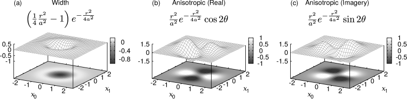
Figure 6: Distortional modes for $k_{0}+k_{1}=2$.

Since $B$ is proportional to $\widetilde{u}_{00}^{2}$, an increase of $\widetilde{u}_{00}/B$ implies a decrease in $\widetilde{u}_{00}$. In Figure 5(a), the slope of $\widetilde{u}_{00}/B$ is discontinuous at about $\widetilde{\beta}B\approx 0.0137$. For $\widetilde{\beta}B\lesssim 0.0137$, the slope is significantly larger than that in the region of $\widetilde{\beta}B\gtrsim 0.0137$. This implies that the motion of a bump helps the bump to maintain its magnitude. It also agrees with the tendency of the average membrane potential (or neuronal activity) profile in 1D CANN that the bump tends to move to a region with a higher concentration of neurotransmitters (York & van Rossum, 2009; Fung et al., 2012a).

Figure 5(c) suggests that an anisotropic mode happens only when the bump is not static, while Figure 5(b) shows that the average width of $u(\mathbf{x},t)$ profile increases with the strength of STD. The behavior of the average change in width, $\left(\widetilde{u}_{20}+\widetilde{u}_{02}\right)$, is similar to that in height. The anisotropic mode happens only when the bump is moving. This suggests that the bump get widened unevenly due to the asymmetric $p(\mathbf{x},t)$ profile.

3.3 Phase Diagram

In the previous subsection, we have shown that the perturbative method can successfully predict different modes of distortions of $\widetilde{u}\left(\mathbf{x},t\right)$ and the intrinsic speed of spontaneous motion. We have also predicted the phase boundary separating translationally stable static bumps and translationally unstable static bumps. To predict different phases in the parameter space, however, we need to study the stability of fixed point solutions given by Eqs. (LABEL:eq:dukkdt), (29) and (30). A detailed discussion of the stability issue can be found in Appendix C.

By studying the stability of fixed point moving solutions, we can obtain a phase boundary separating silent and moving phases, as plotted as a dashed line in Figure 4. In Figure 4, there is a rather complete phase diagram for the model of 2D CANNs with STD we are studying here. For small enough $\widetilde{\beta}$s (below the solid curve in Figure 4), since static bumps are stable in amplitude and translation, this parameter region supports only static bumps. This region is called the static phase.

For parameters between the dotted line and the solid line, static bumps are stable in amplitude but unstable against translational distortions. So in this case, in a rather short time window, both static bumps and moving bumps are able to exist. Because once a translationally unstable static bump get perturbed, it becomes a moving bump. Since both static bumps and moving bumps are observed in this parameter region, we call it the bistable phase. If we further increase $\widetilde{\beta}$, however, even static bump cannot be observed. And only moving bumps can be observed in the parameter region, we call it the moving phase. When both $\widetilde{k}$ and $\widetilde{\beta}$ are large, no non-trivial solution can be found in our analysis or simulations.

In this study we did not find the homogeneous firing patterns reported by York & van Rossum (2009). In the 1D case, however, homogeneous firing can be found in the $\widetilde{k}\rightarrow 0$ regime (Wang et al., Unpublished). Since we are focusing on moderate magnitudes of $\widetilde{k}$, the possibility of uniform firing behavior in 2D CANNs with STD near $\widetilde{k}=0$ is reserved for future studies.

4 CANNs with SFA

4.1 Stationary Solution

By setting $\widetilde{\beta}=0$ in Eq. (5), the CANN model we are considering becomes a network with SFA only. To study the stationary solution in this case, we assume

$$u\left(\mathbf{x}\right)= ~{}u_{00}\exp\left(-\frac{\mathbf{x}^{2}}{4a^{2}}\right),$$ (38)

$$v\left(\mathbf{x}\right)= ~{}v_{00}\exp\left(-\frac{\mathbf{x}^{2}}{4a^{2}}\right).$$ (39)

By substituting Eqs. (38) and (39) into Eqs. (4) and (6), we found that the fixed point solution is given by

$$\widetilde{u}_{00}= ~{}4\frac{1\pm\sqrt{1-\left(1+\gamma\right)^{2}\widetilde{k}}}{\left(1+\gamma\right)\widetilde{k}},$$ (40)

$$\widetilde{v}_{00}= ~{}4\gamma\frac{1\pm\sqrt{1-\left(1+\gamma\right)^{2}\widetilde{k}}}{\left(1+\gamma\right)\widetilde{k}},$$ (41)

$$B= ~{}2\frac{1\pm\sqrt{1-\left(1+\gamma\right)^{2}\widetilde{k}}}{\left(1+\gamma\right)^{2}\widetilde{k}}.$$ (42)

$\widetilde{u}_{00}$ is a rescaled variable defined by $\widetilde{u}_{00}\equiv\rho J_{0}u_{00}$. Similarly, $\widetilde{v}_{00}\equiv\rho J_{0}v_{00}$. We can also rescale $u(\mathbf{x},t)$ and $v(\mathbf{x},t)$ in the same way: i.e., $\widetilde{u}(\mathbf{x},t)\equiv\rho J_{0}u(\mathbf{x},t)$ and $\widetilde{v}(\mathbf{x},t)\equiv\rho J_{0}v(\mathbf{x},t)$. For $\tau_{B}=0$, the fixed point solution with the larger $\widetilde{u}_{00}$ and $\widetilde{v}_{00}$ is stable whenever

$$0<\widetilde{k}<\frac{1+2\gamma}{\left(1+\gamma\right)^{4}},$$ (43)

which is labeled by curve $L$ in Figure 7 for $\widetilde{k}=0.3$. The stability issue can be studied by considering the dynamics of distortions of dynamical variables from their fixed point solutions. Let

$$\widetilde{u}\left(\mathbf{x},t\right)= ~{}\left[\widetilde{u}_{00}+\delta\widetilde{u}_{00}\left(t\right)\right]\exp\left(-\frac{\mathbf{x}^{2}}{4a^{2}}\right),$$ (44)

$$\widetilde{v}\left(\mathbf{x},t\right)= ~{}\left[\widetilde{v}_{00}+\delta\widetilde{v}_{00}\left(t\right)\right]\exp\left(-\frac{\mathbf{x}^{2}}{4a^{2}}\right),$$ (45)

$$B\left(t\right)= ~{}B+\delta B\left(t\right).$$ (46)

By studying the stability of fixed point solutions, we obtain a parameter region for static bumps with stable amplitudes. Detailed analysis of the stability issue can be found in Appendix D. Regions for $\widetilde{k}=0.3$ and various $(\tau_{i}/\tau_{s})$s are shown in Figure 7. For $\tau_{B}>0$, the parameter region over the $(\widetilde{k},\gamma)$ space becomes smaller as $\tau_{B}$ increases. At the $\tau_{i}\gg\tau_{s}$ limit, the range of $\widetilde{k}$ to stabilize the static solution is given by

$$0<\widetilde{k}<\frac{2\gamma+1}{\left(1+\gamma\right)^{4}},$$ (47)

which agrees with Eq. (43). On the other hand, if $\tau_{B}/\tau_{s}\geq 1$, there will be no static solution. In Figure 7, we have shown that if $\gamma$ becomes larger, the maximum value of $\tau_{B}/\tau_{s}$ to stabilize the static solution will be smaller.

Figure 7: Maximum $\tau_{B}/\tau_{s}$ able to stabilize the amplitude of stationary solutions as a function of $\gamma$, given that $\widetilde{k}=0.3$. $L$: maximum $\gamma$ of the existence of stationary solutions.

4.2 Translational Stability

To study the translational stability, we consider the lowest-order asymmetric distortions added to the stationary solution. The major concern here is the step function in Eq. (7), but the step function does not have a first-order effect on translational distortions. We let

$$u\left(\mathbf{x},t\right)= ~{}u_{00}\left(t\right)\exp\left(-\frac{\left|\mathbf{x}\right|^{2}}{4a^{2}}\right),$$ (48)

$$v\left(\mathbf{x},t\right)= ~{}v_{00}\left(t\right)\exp\left(-\frac{\left|\mathbf{x}\right|^{2}}{4a^{2}}\right)+v_{10}\left(t\right)\frac{x_{0}}{a}\exp\left(-\frac{\left|\mathbf{x}\right|^{2}}{4a^{2}}\right).$$ (49)

As we are studying the stability issue of the static solution, let us adopt the solution in Eqs. (40) - (42) and put $v_{10}=0$. Then the dynamics of distortions of dynamical variables near fixed point static solutions becomes

$$\tau_{s}\frac{d}{dt}\left(\begin{array}[]{c}\delta\widetilde{u}_{00}\left(t\right)\\ \delta\widetilde{v}_{00}\left(t\right)\\ \delta B\left(t\right)\\ \delta\widetilde{v}_{10}\left(t\right)\end{array}\right)\\ =\left(\begin{array}[]{cc}\mathscr{A}_{\rm SFA}&0\\ 0&-\frac{\tau_{s}}{\tau_{i}}+\gamma\end{array}\right)\left(\begin{array}[]{c}\delta\widetilde{u}_{00}\left(t\right)\\ \delta\widetilde{v}_{00}\left(t\right)\\ \delta B\left(t\right)\\ \delta\widetilde{v}_{10}\left(t\right)\end{array}\right),$$ (50)

where the $3\times 3$ matrix $\mathscr{A}_{\rm SFA}$ is provided in Appendix D. $\mathscr{A}_{\rm SFA}$ determines amplitudal stability of the static solution. Clearly, the variable $v_{10}$ becomes unstable if $\gamma>\tau_{s}/\tau_{i}$. This implies that if the dynamics of SFA is slow enough, the static solution will be translationally unstable.

4.3 Moving Solution

Once $\gamma>\tau_{s}/\tau_{i}$ is satisfied, spontaneous motion of a bump-shaped solution in 2D CANN with SFA becomes possible. As in the STD case, however, lower-order expansions of $u\left(\mathbf{x},t\right)$ and $p\left(\mathbf{x},t\right)$ are not sufficient to describe the moving solutions. We have to consider higher-order expansions if we want to obtain good predictions on the behavior of moving solutions. Surprisingly, we found that a limited order of expansion of $u\left(\mathbf{x},t\right)$ and $v\left(\mathbf{x},t\right)$ can give some fairly good predictions on the moving solutions.

In general, we consider

$$u\left(\mathbf{x},t\right)= ~{}\sum_{k_{0}k_{1}}u_{k_{0}k_{1}}\left(t\right)\phi_{k_{0}}\left(\xi_{0}\right)\phi_{k_{1}}\left(\xi_{1}\right),$$ (51)

$$v\left(\mathbf{x},t\right)= ~{}\sum_{k_{0}k_{1}}v_{k_{0}k_{1}}\left(t\right)\phi_{k_{0}}\left(\xi_{0}\right)\phi_{k_{1}}\left(\xi_{1}\right).$$ (52)

Here

$$\phi_{k_{i}}\left(\xi_{i}\right)=\frac{1}{\sqrt{\sqrt{2\pi}ak_{i}!}}H_{k_{i}}\left(\frac{\xi_{i}}{a}\right)\exp\left(-\frac{\xi_{i}^{2}}{4a^{2}}\right)$$ (53)

and $H_{k_{i}}$ is the $k_{i}^{\text{th}}$-order probabilist’s Hermite polynomial. Eqs. (40) and (41) become

$$~{}\tau_{s}\frac{d\widetilde{u}_{k_{0}k_{1}}}{dt}\left(t\right)$$

$$= ~{}-\widetilde{u}_{k_{0}k_{1}}\left(t\right)-\widetilde{v}_{k_{0}k_{1}}\left(t\right)+\frac{1}{B\left(t\right)}\sum_{n_{0}n_{1}m_{0}m_{1}}C_{n_{0}m_{0}}^{k_{0}}C_{n_{1}m_{1}}^{k_{1}}\widetilde{u}_{n_{0}n_{1}}\left(t\right)\widetilde{u}_{m{}_{0}m_{1}}\left(t\right),$$

$$~{}\qquad\qquad\qquad-\frac{\tau_{s}c_{0}}{2a}\left[\sqrt{k_{0}}\widetilde{u}_{k_{0}-1,k_{1}}\left(t\right)-\sqrt{k_{0}+1}\widetilde{u}_{k_{0}+1,k_{1}}\left(t\right)\right]$$

$$~{}\qquad\qquad\qquad-\frac{\tau_{s}c_{1}}{2a}\left[\sqrt{k_{1}}\widetilde{u}_{k_{0},k_{1}-1}\left(t\right)-\sqrt{k_{1}+1}\widetilde{u}_{k_{0},k_{1}+1}\left(t\right)\right]$$ (54)

$$~{}\tau_{i}\frac{d\widetilde{v}_{k_{0}k_{1}}}{dt}\left(t\right)$$

$$= ~{}-\widetilde{v}_{k_{0}k_{1}}\left(t\right)+\gamma\widetilde{u}_{k_{0}k_{1}}\left(t\right)$$

$$~{}\qquad\qquad\qquad-\frac{\tau_{i}c_{0}}{2a}\left[\sqrt{k_{0}}\widetilde{v}_{k_{0}-1,k_{1}}\left(t\right)-\sqrt{k_{0}+1}\widetilde{v}_{k_{0}+1,k_{1}}\left(t\right)\right]$$

$$~{}\qquad\qquad\qquad-\frac{\tau_{i}c_{1}}{2a}\left[\sqrt{k_{1}}\widetilde{v}_{k_{0},k_{1}-1}\left(t\right)-\sqrt{k_{1}+1}\widetilde{v}_{k_{0},k_{1}+1}\left(t\right)\right]$$ (55)

Together with the self-consistent condition, Eq. (35), the fixed point solution is solvable. Here the definition of $C_{nm}^{k}$ is not the same as that in Eq. (31), which is defined by

$$C_{nm}^{k}\equiv\int d\xi\phi_{k}\left(\xi\right)\int d\xi^{\prime}\frac{1}{\sqrt{2\pi}a}e^{-\frac{\left(\xi-\xi^{\prime}\right)^{2}}{2a^{2}}}\phi_{n}\left(\xi^{\prime}\right)\phi_{m}\left(\xi^{\prime}\right).$$ (56)

$C_{00}^{0}$ can be calculated explicitly. In general, $C^{k}_{nm}$ can be obtained by using the recurrence relations given in Appendix E.

If we consider only terms up to $k_{0}+k_{1}=2$ and motion along the $x_{0}$-direction, we can obtain the intrinsic speed of the moving solution (detailed derivation can be found in Appendix F):

$$\frac{\tau_{s}\left|c_{0}\right|}{2a}=\frac{\tau_{s}}{\tau_{i}}\sqrt{\frac{1}{3}\left(\frac{\tau_{i}}{\tau_{s}}\gamma-1\right)}.$$ (57)

As the preferred stimulus space is rotationally symmetric, this speed is applicable to motion in any direction. Even though this is an approximated solution with relatively few terms, the prediction on the intrinsic speed is fairly good, as shown in Figure 8.

This result suggests that, in this case, the terms with $k_{0}+k_{1}\leq 2$ are sufficient to give some good predictions on the behavior of bump-shaped solutions. For predictions on measurements of different components of the moving bump, however, we still need to use higher-order perturbation. In Figures 9(a) - (c), we have shown that higher-order perturbation is needed to predict $\widetilde{u}_{k_{0}k_{1}}/B$ if the bump is moving. As in Figures 5(b) and 5(c), in Figures 9(b) and 9(c), we do not compare $\widetilde{u}_{20}$, $\widetilde{u}_{02}$ and $\widetilde{u}_{11}$ directly. Since a moving bump can move in any directions, we compare their projections in polar coordinates. Let us consider $\xi_{0}=r\cos\theta$ and $\xi_{1}=r\sin\theta$. Then we have

$$~{}\widetilde{u}_{20}\phi_{2}\left(\xi_{0}\right)\phi_{0}\left(\xi_{1}\right)+\widetilde{u}_{02}\phi_{0}\left(\xi_{0}\right)\phi_{2}\left(\xi_{1}\right)+\widetilde{u}_{11}\phi_{1}\left(\xi_{0}\right)\phi_{1}\left(\xi_{1}\right)$$

$$= ~{}\left(\widetilde{u}_{20}+\widetilde{u}_{02}\right)\frac{1}{2a\sqrt{\pi}}\left(\frac{1}{2}\frac{r^{2}}{a^{2}}-1\right)e^{-\frac{r^{2}}{4a^{2}}}+\left(\widetilde{u}_{20}-\widetilde{u}_{02}-\sqrt{2}i\widetilde{u}_{11}\right)\frac{1}{8a\sqrt{\pi}}\frac{r^{2}}{a^{2}}e^{-\frac{r^{2}}{4a^{2}}}e^{i2\theta}$$

$$~{}+\left(\widetilde{u}_{20}-\widetilde{u}_{02}+\sqrt{2}i\widetilde{u}_{11}\right)\frac{1}{8a\sqrt{\pi}}\frac{r^{2}}{a^{2}}e^{-\frac{r^{2}}{4a^{2}}}e^{-i2\theta}.$$ (58)

In Figures 9(b) and 9(c), we compare predictions and simulation results of $\left(\widetilde{u}_{20}+\widetilde{u}_{02}\right)$ and $\left|\widetilde{u}_{20}-\widetilde{u}_{02}-\sqrt{2}i\widetilde{u}_{11}\right|$ for $k_{0}+k_{1}=2$ and $k_{0}+k_{1}=10$. $\left(\widetilde{u}_{20}+\widetilde{u}_{02}\right)$ is the average change in the width of the bump-shaped profile, while $\left|\widetilde{u}_{20}-\widetilde{u}_{02}-\sqrt{2}i\widetilde{u}_{11}\right|$ is the magnitude of the anisotropic mode. The graphical illustration of Eq. (58) is omitted because it is similar to the illustrations shown in Figure 6.

The behavior of moving solutions of CANNs with SFA is similar to that of moving solutions of CANNs with STD. For $\widetilde{u}_{00}/B$, its trend is basically the same as $\widetilde{u}_{00}/B$ in the case with STD shown in Figure 5. The transition happens whenever $\gamma=\tau_{s}/\tau_{i}$. Also, anisotropic modes will be available only when the bump is moving, while the width of the $u(\mathbf{x},t)$ profile increases as the strength of SFA increases. The behavior of the average change in width is similar to the behavior of the change in height, $\widetilde{u}_{00}$. The dependence of anisotropic modes on the strength of SFA, $\gamma$, implies that the widening effect is not uniform when the bump is moving, which is similar to what is seen in a 2D CANN with STD.

Figure 8: Speed of spontaneous motions as a function of $\gamma$.

Figure 9: (a) Projection of $\widetilde{u}\left(\mathbf{x},t\right)$ on $\phi_{0}\left(\xi_{0}\right)\phi_{0}\left(\xi_{1}\right)$. (b) Projection of $\widetilde{u}\left(\mathbf{x},t\right)$ on rotationally symmetric basis function with $k_{0}+k_{1}=2$. (c) Projection of $\widetilde{u}\left(\mathbf{x},t\right)$ on anisotropic basis function with $k_{0}+k_{1}=2$. (a) - (c) Parameters: $a=0.5$, $\tau_{i}/\tau_{s}=10$ and $\tau_{B}/\tau_{s}=0.1$.

Figure 10: Phase diagram over the parameter space spanned by $\left(\widetilde{k},\gamma\right)$. Dotted line: boundary predicted for moving solutions by $k_{0}+k_{1}=2$ perturbation. Solid line: boundary predicted for moving solutions by $k_{0}+k_{1}=10$ perturbation. Dotted line: boundary predicted for static solutions with stable amplitudes by $k_{0}+k_{1}=0$ perturbation. Dot-dashed line: boundary predicted for static solutions with stable amplitudes and translational stability by $k_{0}+k_{1}=0$ perturbation. Parameters: same as Figure 9. Symbols: corresponding simulations.

4.4 Phase Diagram

A phase diagram similar to Figure 4 for SFA can be obtained in a similar manner used for CANNs with STD. In the previous subsection, we have shown that perturbative analysis is able to predict dynamical variables of the model. By solving for the moving solutions numerically and testing their stability, we can predict the phase boundary separating parameter regions for moving solutions and trivial solution (silent phase). Using it together with the stability conditions for static bumps given in Eqs. (43) and (50), we can predict the phase diagram for SFA. We found that the predicted phase diagram matches the phase diagram obtained from computer simulations (Figure 10). As in Figure 4, there are four phases in the phase diagram: a static phase, a bistable phase, a moving phase and a silent phase. Their meanings are the same as those of their counterparts in Figure 4. Remarkably, expansions up to $k_{0}+k_{1}=2$ can also predict the phase diagram well, which is similar to the prediction of intrinsic speed of moving bumps in CANNs with SFA.

5 Discussion

5.1 Intrinsic Phases and Phase Diagrams

In the parameter spaces of the two models we studied in this paper, there are static, bistable, moving and silent phases. When $\widetilde{\beta}$ is large enough, moving bumps can be found in bistable phase and moving phase. This behavior can also be seen in the case of SFA. In both STD and SFA cases, whenever $\widetilde{\beta}$ or $\gamma$ is not too large (within the bistable phase), static bumps can still exist for a not insignificant period of time. If $\widetilde{\beta}$ or $\gamma$ is too large, only trivial solutions are stable.

Behaviors of CANNs with STD are very similar to those of CANNs with SFA. This suggests that multiplicative dynamical suppression mechanisms (represented by STD) and subtractive dynamical suppression mechanisms (represented by SFA) can generate similar intrinsic dynamics, especially with regard to spontaneous motion. It also implies that other smooth models having homogeneous couplings and dynamical suppression mechanisms should have a similar phase diagram consisting of static, moving, bistable and silent phases.

In some studies on CANNs with STD or SFA it is reported that, with some parameters, uniform firing pattern can be found in the network (e.g. York & van Rossum, 2009). In the present study, uniform firing is not included because the interactive range of the global inhibition in this model is infinite. So uniform firing may only be found in a tight parameter region near $\widetilde{k}\rightarrow 0$. For the 1D STD case, uniform firing can be found in a region $\widetilde{\beta}\rightarrow 0$ and $\widetilde{k}\rightarrow 0$ (Wang et al., Unpublished). Uniform firing should also be found in 2D CANNs with STD or SFA, as should spiral waves and breathing wavefronts. There is a report on spiral waves and breathing wavefronts in 2D CANNs with STD (e.g. Kilpatrick & Bressloff, 2010a), but those phenomena are missing from the phase diagram we predicted because spiral waves and breathing wavefronts are not local patterns. Therefore in the present model they may exist if the magnitude of divisive global inhibition is very small. Richer dynamics of the present model for $\widetilde{k}\rightarrow 0$ is reserved for future investigations.

5.2 Effectiveness of Perturbative Approach

In this paper we have shown that, in the present particular model, the perturbative expansion method is applicable to the study of continuous attractor neural networks (CANNs) with short-term synaptic depression (STD) or spike frequency adaptation (SFA). We found in this study that both STD and SFA can drive similar intrinsic dynamics of the local neural activity profile. In Figures 4 and 10 there are four phases: silent, static, bistable and moving. Using perturbative expansions on the dynamical variables, we can successfully predict the phase diagrams in both cases with STD and SFA.

As expected, with low-order expansions (i.e., when $k_{0}+k_{1}$ is small), predictions on $\widetilde{u}_{k_{0}k_{1}}$’s of the static solutions work well in cases with STD and SFA. For moving solutions, higher-order expansions are needed to obtain more accurate solutions. In Figures 5(a) - (c) and Figure 9 it is shown that low-order perturbative expansions, $k_{0}+k_{1}=3$ for STD and $k_{0}+k_{1}=2$ for SFA, are able to show the general trend of dynamical variables. Especially, the second-order transitions in all the dynamical variables (i.e. discontinuities of slopes) are observed at this level of perturbative expansion. This suggests that low-order perturbative expansions are good enough for studying general phenomena in different phases.

To predict the behavior of the dynamical variables more accurately, we need to use higher-order perturbative expansions. We have shown in Figures 5(a) - (c) and Figure 9 that higher-order perturbative expansions, $k_{0}+k_{1}=11$ for STD and $k_{0}+k_{1}=10$ for SFA, can fit measurements from simulations accurately. Higher-order terms do not, however, significantly improve prediction of the speed of spontaneous motion. This suggests that lower-order perturbative modes are most important to the motion of the local neural activity profile.

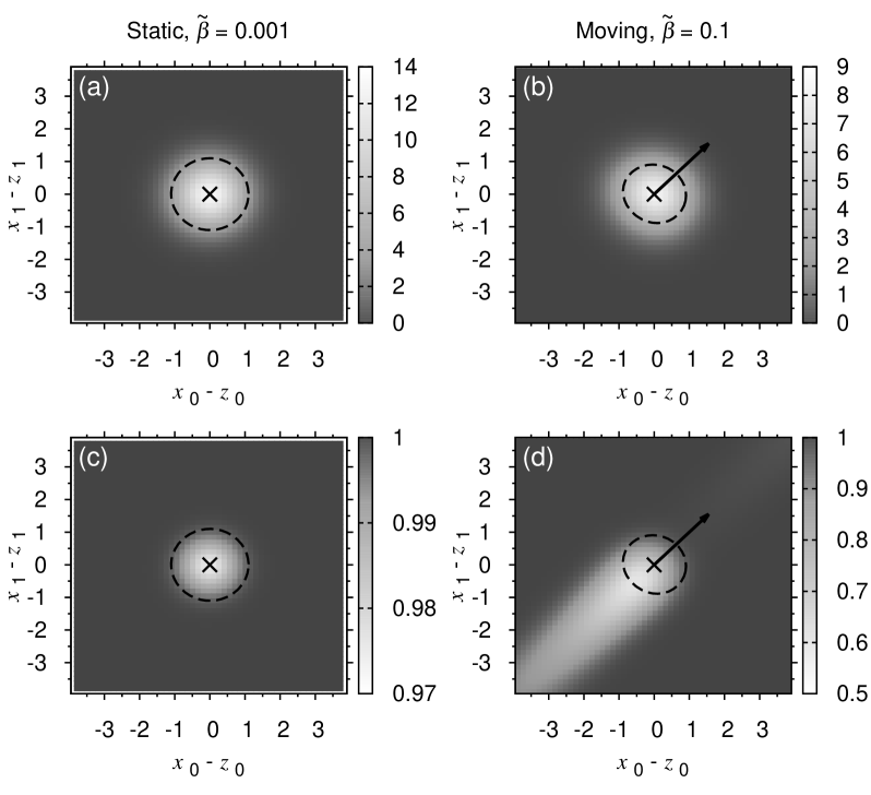
Figure 11: Snapshots of $\widetilde{u}\left(\mathbf{x},t\right)$ and $p\left(\mathbf{x},t\right)$ in the static phase ((a) and (c)) and moving phase ((b) and (d)). (a) and (b) are $\widetilde{u}\left(\mathbf{x},t\right)$, while (c) and (d) are $p\left(\mathbf{x},t\right)$. Dashed lines: contours for $\widetilde{u}\left(\mathbf{x},t\right)=4$. $\left(z_{0},z_{1}\right)$ is the center of mass of $\widetilde{u}\left(\mathbf{x},t\right)$. The moving direction of the bump is the $\left(1,1\right)$ direction, shows by the arrows in (b) and (d). Parameters: $\widetilde{k}=0.5$, $\tau_{d}/\tau_{s}=50$ and $\widetilde{\beta}=0.001$ for (a) and (c), and $\widetilde{\beta}=0.1$ for (b) and (d).

5.3 Asymmetric Modes and Moving Solutions

Higher-order perturbative modes are essential for predicting the behavior of dynamical variables of moving solutions accurately because the dynamical variables will become asymmetric about the center of mass of $\widetilde{u}\left(\mathbf{x},t\right)$ if the neural activity profile is moving. In Figure 11, there are two examples of CANNs with different levels of STD. Figures 11(a) and 11(c) are with $\widetilde{\beta}=0.001$, which corresponds to the static phase. In this case, both the average membrane potential profile $\widetilde{u}\left(\mathbf{x},t\right)$ and the fraction of available neurotransmitters $p\left(\mathbf{x},t\right)$ are rotationally symmetric about the center of mass of $\widetilde{u}\left(\mathbf{x},t\right)$. Therefore, in the static phase, low-order perturbation is good enough for making predictions.

Snapshots of $\widetilde{u}\left(\mathbf{x},t\right)$ and $p\left(\mathbf{x},t\right)$ in the moving phase are shown in Figures 11(b) and 11(d). Here the level of STD is $\widetilde{\beta}=0.1$. In this case, $\widetilde{u}\left(\mathbf{x},t\right)$ seems to be rotationally symmetric about its center of mass. Actually, the shape of the Gaussian-like average membrane potential profile is slightly squeezed along the moving direction. For $p\left(\mathbf{x},t\right)$, however, the deformation of the shape is more significant. In Figure 11(d), the profile of $p\left(\mathbf{x},t\right)$ is strongly biased against the moving direction. This highly skewed profile of $p\left(\mathbf{x},t\right)$ makes high-order perturbative mode more important, especially for cases involving stability and predictions of dynamical variables.

5.4 Limitation of Perturbative Approach

In this paper, we have shown the perturbative approach is able to successfully predict 1) the phase diagrams of CANNs with STD or SFA, 2) the speed of spontaneous motion and 3) the dynamical variables (e.g. $\widetilde{u}\left(x,t\right)$). Phenomena richer than spontaneous motion of local neural activity, for example, breathing wavefronts on neural networks have been considered theoretically (Kilpatrick & Bressloff, 2010a). The perturbative formulation is not applicable in that case, however, because the basis function we used here are local, while the traveling wavefronts are globally spreading. For the same reason, this method cannot be used to analyze also spiral waves on a 2D field.

In the case of collisions of two moving bump-shaped profiles of neuronal activity, one may find the dynamics hard to analyze by the perturbative method. This is because there are two centers of mass, one for each bump, and this makes the choice of the origin of basis functions confusing. For example, if one chose one of the centers of mass to be the origin of basis functions, the chosen family of basis functions will not be optimal for the other bump and will make the expansion of that bump less efficient.

Conclusion

In this paper we studied models with short-term synaptic depression and spike frequency adaptation and these models which was based on a two-dimensional CANN model with divisive global inhibition. We found that their intrinsic dynamics were similar. First, there are four phases in each scenario. They are static, moving, bistable and silent. The moving phase is the phase in which the bump-shaped profile moves spontaneously, while the static phase is the phase in which the bump-shaped profile cannot move spontaneously. Interestingly, in the bistable phase, the CANN can support both moving profiles and static profiles.

Second, there are clear phase transitions between static solutions and moving solutions. In Figures 5, 8 and 9 there is a clear discontinuity in slope between the two states. This suggests that, spontaneous motion can affect the shapes of the bump-shaped profiles.

The stability of steady states, the shapes of the dynamical variables and the speed of spontaneous motion can be predicted by perturbative analysis, but perturbative method cannot be used in some scenarios including spiral waves, breathing wavefronts and collisions of multiple bumps in 2D fields.

Acknowledgments

This study is partially supported by the Research Grants Council of Hong Kong (grant numbers 604512, 605813 and N_HKUST 606/12).

Appendix

A Amplitudal Stability of Bumps on 2D CANNs with STD

To study the stability of fixed point solutions of Eqs. (14) - (16), we assume

$$\widetilde{u}_{00}\left(t\right)= ~{}\widetilde{u}_{00}^{*}+\delta\widetilde{u}_{00}\left(t\right),$$ (A.1)

$$p_{00}\left(t\right)= ~{}p_{00}^{*}+\delta p_{00}\left(t\right),$$ (A.2)

$$B\left(t\right)= ~{}B^{*}+\delta B\left(t\right).$$ (A.3)

Linearizing Eqs. (14) - (16), we obtain

$$\tau_{s}\frac{d}{dt}\left(\begin{array}[]{c}\widetilde{u}_{00}\left(t\right)\\ p_{00}\left(t\right)\\ B\left(t\right)\end{array}\right)=\mathscr{A}_{\rm STD}\left(\begin{array}[]{c}\widetilde{u}_{00}\left(t\right)\\ p_{00}\left(t\right)\\ B\left(t\right),\end{array}\right)$$ (A.4)

where

$$\mathscr{A}_{\rm STD}= ~{}\left(\begin{array}[]{ccc}\frac{\partial F_{\widetilde{u}_{00}}\left(\widetilde{u}_{00},p_{00},B\right)}{\partial\widetilde{u}_{00}}&\frac{\partial F_{\widetilde{u}_{00}}\left(\widetilde{u}_{00},p_{00},B\right)}{\partial p_{00}}&\frac{\partial F_{\widetilde{u}_{00}}\left(\widetilde{u}_{00},p_{00},B\right)}{\partial B}\\ \frac{\partial F_{p_{00}}\left(\widetilde{u}_{00},p_{00},B\right)}{\partial\widetilde{u}_{00}}&\frac{\partial F_{p_{00}}\left(\widetilde{u}_{00},p_{00},B\right)}{\partial p_{00}}&\frac{\partial F_{p_{00}}\left(\widetilde{u}_{00},p_{00},B\right)}{\partial B}\\ \frac{\partial F_{B}\left(\widetilde{u}_{00},p_{00},B\right)}{\partial\widetilde{u}_{00}}&\frac{\partial F_{B}\left(\widetilde{u}_{00},p_{00},B\right)}{\partial p_{00}}&\frac{\partial F_{B}\left(\widetilde{u}_{00},p_{00},B\right)}{\partial B}\end{array}\right)$$ (A.8)

$$= ~{}\left(\begin{array}[]{ccc}-1+\frac{1}{B}\widetilde{u}_{00}\left(1-\frac{4}{7}\widetilde{p}_{00}\right)&-\frac{2}{7}\frac{1}{B}\widetilde{u}_{00}^{2}&-\frac{1}{2}\frac{1}{B^{2}}\widetilde{u}_{00}^{2}\left(1-\frac{4}{7}\widetilde{p}_{00}\right)\\ \frac{2\tau_{s}}{\tau_{d}}\frac{\widetilde{\beta}}{B}\widetilde{u}_{00}\left(1-\frac{2}{3}\widetilde{p}_{00}\right)&-\frac{\tau_{s}}{\tau_{d}}-\frac{2}{3}\frac{\tau_{s}}{\tau_{d}}\frac{\widetilde{\beta}}{B}\widetilde{u}_{00}^{2}&-\frac{\tau_{s}}{\tau_{d}}\frac{\widetilde{\beta}}{B^{2}}\widetilde{u}_{00}^{2}\left(1-\frac{2}{3}\widetilde{p}_{00}\right)\\ \frac{1}{8}\frac{\tau_{s}}{\tau_{B}}\widetilde{k}\widetilde{u}_{00}&0&-\frac{\tau_{s}}{\tau_{B}}\end{array}\right),$$ (A.12)

and

$$F_{\widetilde{u}_{00}}\left(\widetilde{u}_{00},p_{00},B\right)\equiv ~{}-\widetilde{u}_{00}+\frac{1}{2}\frac{1}{B}\widetilde{u}_{00}^{2}\left[1-\frac{4}{7}p_{00}\right],$$ (A.13)

$$F_{p_{00}}\left(\widetilde{u}_{00},p_{00},B\right)\equiv ~{}\frac{\tau_{s}}{\tau_{d}}\left\{-p_{00}+\frac{1}{B}\widetilde{\beta}\widetilde{u}_{00}^{2}\left[1-\frac{2}{3}p_{00}\right]\right\},$$ (A.14)

$$F_{B}\left(\widetilde{u}_{00},p_{00},B\right)\equiv ~{}\frac{\tau_{s}}{\tau_{B}}\left[-B+1+\frac{1}{16}\widetilde{k}\widetilde{u}_{00}^{2}\right].$$ (A.15)

By calculating eigenvalues of this matrix for a given fixed point solution, we can test the stability of each solution. In Figure 3 the parabolas are plotted from $\widetilde{\beta}=0$ to a point such that the real part of one of the eigenvalues just turns positive. The solid line in Figure 3 maps the parameter region for the existence of static profiles of $u(\mathbf{x},t)$.

For the stability matrix in Eq. (21), since $p_{10}=0$ for static states, amplitudal stability and translational stability are uncoupled. The $\mathscr{A}_{\rm STD}$ in the $4\times 4$ matrix in Eq. (21) is the same as that given in Eq. (A.8).

B Derivations of Eqs. (LABEL:eq:dukkdt) - (30)

To obtain Eqs. (LABEL:eq:dukkdt) - (30), we need to deal with differentiations of basis functions $\psi_{k}\left(\xi\right)$ and $\varphi_{k}\left(\xi\right)$:

$$\frac{d\psi_{k}\left(\xi\right)}{d\xi}= ~{}\frac{1}{2a}\sqrt{k}\psi_{k-1}\left(\xi\right)-\frac{1}{2a}\sqrt{k+1}\psi_{k-1}\left(\xi\right)$$ (B.1)

$$\frac{d\varphi_{k}\left(\xi\right)}{d\xi}= ~{}\frac{1}{\sqrt{2}a}\sqrt{k}\varphi_{k-1}\left(\xi\right)-\frac{1}{\sqrt{2}a}\sqrt{k+1}\varphi_{k-1}\left(\xi\right)$$ (B.2)

Combining this result with Eqs. (24), (25), we have

$$\tau_{s}\frac{\partial\widetilde{u}\left(\boldsymbol{\xi},t\right)}{\partial t}= ~{}\tau_{s}\sum_{k_{0}k_{1}}\biggl{\{}\frac{d\widetilde{u}_{k_{0}k_{1}}\left(t\right)}{dt}-\frac{c_{0}}{2a}\left[\sqrt{k_{0}+1}\widetilde{u}_{k_{0}+1,k_{1}}\left(t\right)-\sqrt{k_{0}}\widetilde{u}_{k_{0}-1,k_{1}}\left(t\right)\right]\biggr{.}$$

$$~{}\biggl{.}\frac{c_{1}}{2a}\left[\sqrt{k_{1}+1}\widetilde{u}_{k_{0},k_{1}+1}\left(t\right)-\sqrt{k_{1}}\widetilde{u}_{k_{0},k_{1}-1}\left(t\right)\right]\biggr{\}}\psi_{k_{0}}\left(\xi_{0}\right)\psi_{k_{1}}\left(\xi_{1}\right)$$ (B.3)

$$\tau_{d}\frac{\partial p\left(\boldsymbol{\xi},t\right)}{\partial t}= ~{}-\tau_{d}\sum_{k_{0}k_{1}}\biggl{\{}\frac{dp_{k_{0}k_{1}}\left(t\right)}{dt}-\frac{c_{0}}{\sqrt{2}a}\left[\sqrt{k_{0}+1}p_{k_{0}+1,k_{1}}\left(t\right)-\sqrt{k_{0}}p_{k_{0}-1,k_{1}}\left(t\right)\right]\biggr{.}$$

$$~{}\biggl{.}\frac{c_{1}}{\sqrt{2}a}\left[\sqrt{k_{1}+1}p_{k_{0},k_{1}+1}\left(t\right)-\sqrt{k_{1}}p_{k_{0},k_{1}-1}\left(t\right)\right]\biggr{\}}\varphi_{k_{0}}\left(\xi_{0}\right)\varphi_{k_{1}}\left(\xi_{1}\right)$$ (B.4)

We now obtain the left-hand sides of Eqs. (4) and (5). For the right-hand sides, by substituting Eqs. (24) and (25) into right-hand sides of Eqs. (4) and (5) and projecting them onto corresponding basis functions, we obtain

$$~{}-\widetilde{u}\left(\mathbf{x},t\right)+\frac{1}{B\left(t\right)}\int d\mathbf{x}\widetilde{J}\left(\left|\mathbf{x}-\mathbf{x}^{\prime}\right|\right)p\left(\mathbf{x}^{\prime},t\right)\widetilde{u}\left(\mathbf{x}^{\prime},t\right)^{2}$$

$$= ~{}\sum_{k_{0}k_{1}}\widetilde{u}_{k_{0}k_{1}}\psi_{k_{0}}\left(\xi_{0}\right)\psi_{k_{1}}\left(\xi_{1}\right)$$

$$~{}+\frac{1}{B\left(t\right)}\sum_{k_{0}k_{1}}\psi_{k_{0}}\left(\xi_{0}\right)\psi_{k_{1}}\left(\xi_{1}\right)\left(\sum_{n_{0}n_{1}m_{0}m_{1}}C_{n_{0}m_{0}}^{k_{0}}C_{n_{1}m_{1}}^{k_{1}}\widetilde{u}_{n_{0}n_{1}}\widetilde{u}_{m_{0}m_{1}}\right)$$

$$~{}-\frac{1}{B\left(t\right)}\sum_{k_{0}k_{1}}\psi_{k_{0}}\left(\xi_{0}\right)\psi_{k_{1}}\left(\xi_{1}\right)\left(\sum_{n_{0}n_{1}m_{0}m_{1}l_{0}l_{1}}D_{n_{0}m_{0}l_{0}}^{k_{0}}D_{n_{1}m_{1}l_{1}}^{k_{1}}\widetilde{u}_{n_{0}n_{1}}\widetilde{u}_{m_{0}m_{1}}p_{l_{0}l_{1}}\right),$$

$$~{}1-p\left(\mathbf{x},t\right)-\tau_{d}\beta p\left(\mathbf{x},t\right)\frac{\widetilde{u}\left(\mathbf{x},t\right)^{2}}{B\left(t\right)}$$

$$= ~{}\sum_{k_{0}k_{1}}p_{k_{0}k_{1}}\left(t\right)\varphi_{k_{0}}\left(\xi_{0}\right)\varphi_{k_{1}}\left(\xi_{1}\right)$$

$$~{}-\frac{\tau_{d}\beta}{B\left(t\right)}\sum_{k_{0}k_{1}}\varphi_{k_{0}}\left(\xi_{0}\right)\varphi_{k_{1}}\left(\xi_{1}\right)\left(\sum_{n_{0}n_{1}m_{0}m_{1}}E_{n_{0}m_{0}}^{k_{0}}E_{n_{1}m_{1}}^{k_{1}}\widetilde{u}_{n_{0}n_{1}}\widetilde{u}_{m_{0}m_{1}}\right)$$

$$~{}+\frac{\tau_{d}\beta}{B\left(t\right)}\sum_{k_{0}k_{1}}\varphi_{k_{0}}\left(\xi_{0}\right)\varphi_{k_{1}}\left(\xi_{1}\right)\left(\sum_{n_{0}n_{1}m_{0}m_{1}}F_{n_{0}m_{0}l_{0}}^{k_{0}}F_{n_{1}m_{1}l_{1}}^{k_{1}}\widetilde{u}_{n_{0}n_{1}}\widetilde{u}_{m_{0}m_{1}}p_{l_{0}l_{1}}\right).$$ (B.6)

Here argument $t$ of $\widetilde{u}_{k_{0}k_{1}}$ and $p_{k_{0}k_{1}}$ are omitted. $\widetilde{J}\left(\left|\mathbf{x}-\mathbf{x}^{\prime}\right|\right)\equiv J_{0}^{-1}J\left(\left|\mathbf{x}-\mathbf{x}^{\prime}\right|\right)$. Combining expressions of the left-hand and right-hand sides of Eqs. (4) and (5), we should obtain Eqs. (LABEL:eq:dukkdt) and (29). Eq. (30) can be obtained easily by substituting Eq. (24) into Eq. (2) and making use of the orthogonality of $\psi_{k_{i}}\left(\xi_{i}\right)$’s.

C Stability of Moving Bumps on 2D CANNs with STD

To study the stability issue, let us define

$$F\left(\widetilde{u}_{00},\cdots,p_{00},\cdots,B|\widetilde{u}_{k_{0}k_{1}}\right)\equiv ~{}-\widetilde{u}_{k_{0}k_{1}}+\frac{\tau_{s}c_{0}}{2a}\left[\sqrt{k_{0}+1}\widetilde{u}_{k_{0}+1,k_{1}}-\sqrt{k_{0}}\widetilde{u}_{k_{0}-1,k_{1}}\right]$$

$$~{}+\frac{\tau_{s}c_{1}}{2a}\left[\sqrt{k_{1}+1}\widetilde{u}_{k_{0},k_{1}+1}-\sqrt{k_{1}}\widetilde{u}_{k_{0},k_{1}-1}\right]$$

$$~{}+\frac{1}{B}\sum_{n_{0}n_{1}m_{0}m_{1}}C_{n_{0}m_{0}}^{k_{0}}C_{n_{1}m_{1}}^{k_{1}}\widetilde{u}_{n_{0}n_{1}}\widetilde{u}_{m_{0}m_{1}}$$

$$~{}-\frac{1}{B}\sum_{n_{0}n_{1}m_{0}m_{1}l_{0}l_{1}}D_{n_{0}m_{0}l_{0}}^{k_{0}}D_{n_{1}m_{1}l_{1}}^{k_{1}}\widetilde{u}_{n_{0}n_{1}}\widetilde{u}_{m_{0}m_{1}}p_{l_{0}l_{1}},$$

$$F\left(\widetilde{u}_{00},\cdots,p_{00},\cdots,B|p_{k_{0}k_{1}}\right)\equiv ~{}\frac{\tau_{s}}{\tau_{d}}\Biggl{\{}-p_{k_{0}k_{1}}\Biggr{.}$$

$$~{}+\frac{\tau_{d}c_{0}}{\sqrt{2}a}\left[\sqrt{k_{0}+1}p_{k_{0}+1,k_{1}}-\sqrt{k_{0}}p_{k_{0}-1,k_{1}}\right]$$

$$~{}+\frac{\tau_{d}c_{1}}{\sqrt{2}a}\left[\sqrt{k_{1}+1}p_{k_{0},k_{1}+1}-\sqrt{k_{1}}p_{k_{0},k_{1}-1}\right]$$

$$~{}+\frac{\widetilde{\beta}}{B}\sum_{n_{0}n_{1}m_{0}m_{1}}E_{n_{0}m_{0}}^{k_{0}}E_{n_{1}m_{1}}^{k_{1}}\widetilde{u}_{n_{0}n_{1}}\widetilde{u}_{m_{0}m_{1}}$$

$$~{}\Biggl{.}-\frac{\widetilde{\beta}}{B}\sum_{n_{0}n_{1}m_{0}m_{1}l_{0}l_{1}}F_{n_{0}m_{0}l_{0}}^{k_{0}}F_{n_{1}m_{1}l_{1}}^{k_{1}}\widetilde{u}_{n_{0}n_{1}}\widetilde{u}_{m_{0}m_{1}}p_{l_{0}l_{1}}\Biggr{\}},$$

$$F\left(\widetilde{u}_{00},\cdots,p_{00},\cdots,B|B\right)\equiv ~{}\frac{\tau_{s}}{\tau_{B}}\Biggl{(}-B+1+\frac{1}{32\pi a^{2}}\widetilde{k}\sum_{k_{0}k_{1}}\widetilde{u}_{k_{0}k_{1}}^{2}\Biggr{)}.$$ (C.3)

The stability of fixed point solutions can be determined by considering the stability matrix given by

$$~{}\mathscr{A}_{\rm STD}^{\rm moving}$$

$$\equiv ~{}\left(\begin{array}[]{ccccc}\frac{\partial F\left(\widetilde{u}_{00},\cdots,p_{00},\cdots,B|\widetilde{u}_{00}\right)}{\partial\widetilde{u}_{00}}&\cdots&\frac{\partial F\left(\widetilde{u}_{00},\cdots,p_{00},\cdots,B|\widetilde{u}_{00}\right)}{\partial p_{00}}&\cdots&\frac{\partial F\left(\widetilde{u}_{00},\cdots,p_{00},\cdots,B|\widetilde{u}_{00}\right)}{\partial B}\\ \vdots&\ddots&\vdots&\ddots&\vdots\\ \frac{\partial F\left(\widetilde{u}_{00},\cdots,p_{00},\cdots,B|p_{00}\right)}{\partial\widetilde{u}_{00}}&\cdots&\frac{\partial F\left(\widetilde{u}_{00},\cdots,p_{00},\cdots,B|p_{00}\right)}{\partial p_{00}}&\cdots&\frac{\partial F\left(\widetilde{u}_{00},\cdots,p_{00},\cdots,B|p_{00}\right)}{\partial B}\\ \vdots&\ddots&\vdots&\ddots&\vdots\\ \frac{\partial F\left(\widetilde{u}_{00},\cdots,p_{00},\cdots,B|B\right)}{\partial\widetilde{u}_{00}}&\cdots&\frac{\partial F\left(\widetilde{u}_{00},\cdots,p_{00},\cdots,B|B\right)}{\partial p_{00}}&\cdots&\frac{\partial F\left(\widetilde{u}_{00},\cdots,p_{00},\cdots,B|B\right)}{\partial B}\end{array}\right).$$ (C.9)

For dynamical variables near their fixed point solutions, we let

$$\widetilde{u}_{k_{0}k_{1}}\left(t\right)\equiv ~{}\widetilde{u}_{k_{0}k_{1}}^{*}+\delta\widetilde{u}_{k_{0}k_{1}}\left(t\right),$$ (C.11)

$$p_{k_{0}k_{1}}\left(t\right)\equiv ~{}p_{k_{0}k_{1}}^{*}+\delta p_{k_{0}k_{1}}\left(t\right),$$ (C.12)

$$B\left(t\right)\equiv ~{}B^{*}+\delta B\left(t\right),$$ (C.13)

where $\widetilde{u}_{k_{0}k_{1}}^{*}$, $p_{k_{0}k_{1}}^{*}$ and $B^{*}$ is the fixed point solution. Then the dynamics of $\delta\widetilde{u}_{k_{0}k_{1}}\left(t\right)$, $\delta p_{k_{0}k_{1}}\left(t\right)$ and $\delta B\left(t\right)$ can be formulated as

$$\tau_{s}\frac{d}{dt}\left(\begin{array}[]{c}\delta\widetilde{u}_{00}\left(t\right)\\ \vdots\\ \delta p_{00}\left(t\right)\\ \vdots\\ \delta B\left(t\right)\end{array}\right)=\mathscr{A}_{\rm STD}^{\rm moving}\left(\begin{array}[]{c}\delta\widetilde{u}_{00}\left(t\right)\\ \vdots\\ \delta p_{00}\left(t\right)\\ \vdots\\ \delta B\left(t\right)\end{array}\right).$$ (C.14)

The fixed point solution is stable only if the maximum of the real parts of eigenvalues of
$\left.\mathscr{A}_{\rm STD}^{\rm moving}\right|_{\widetilde{u}_{00}^{*},\dots,p_{00}^{*},\dots,B^{*}}$ is non-positive. In general, those eigenvalues can only be calculated by numerical methods. The predicted phase boundary separating the moving and silent phases shown in Figure 4 can be deduced, and the prediction can be verified by simulations.

D Amplitudal Stability of Bumps on 2D CANNs with SFA

For our convenience we define

$$K_{\widetilde{u}_{00}}\left(\widetilde{u}_{00},\widetilde{v}_{00},B\right)\equiv ~{}-\widetilde{u}_{00}+\frac{1}{2}\frac{\widetilde{u}_{00}^{2}}{B}-\widetilde{v}_{00},$$ (D.1)

$$K_{\widetilde{v}_{00}}\left(\widetilde{u}_{00},\widetilde{v}_{00},B\right)\equiv ~{}\frac{\tau_{s}}{\tau_{i}}\left(-\widetilde{v}_{00}+\gamma\widetilde{u}_{00}\right),$$ (D.2)

$$K_{B}\left(\widetilde{u}_{00},\widetilde{v}_{00},B\right)\equiv ~{}\frac{\tau_{s}}{\tau_{i}}\left(-B+1+\frac{1}{16}\widetilde{k}\widetilde{u}_{00}^{2}\right).$$ (D.3)

Then the stability matrix is given by

$$\mathscr{A}_{\rm SFA}= ~{}\left(\begin{array}[]{ccc}\frac{\partial K_{\widetilde{u}_{00}}\left(\widetilde{u}_{00},\widetilde{v}_{00},B\right)}{\partial\widetilde{u}_{00}}&\frac{\partial K_{\widetilde{u}_{00}}\left(\widetilde{u}_{00},\widetilde{v}_{00},B\right)}{\partial\widetilde{v}_{00}}&\frac{\partial K_{\widetilde{u}_{00}}\left(\widetilde{u}_{00},\widetilde{v}_{00},B\right)}{\partial B}\\ \frac{\partial K_{\widetilde{v}_{00}}\left(\widetilde{u}_{00},\widetilde{v}_{00},B\right)}{\partial\widetilde{u}_{00}}&\frac{\partial K_{\widetilde{v}_{00}}\left(\widetilde{u}_{00},\widetilde{v}_{00},B\right)}{\partial\widetilde{v}_{00}}&\frac{\partial K_{\widetilde{v}_{00}}\left(\widetilde{u}_{00},\widetilde{v}_{00},B\right)}{\partial B}\\ \frac{\partial K_{B}\left(\widetilde{u}_{00},\widetilde{v}_{00},B\right)}{\partial\widetilde{u}_{00}}&\frac{\partial K_{B}\left(\widetilde{u}_{00},\widetilde{v}_{00},B\right)}{\partial\widetilde{v}_{00}}&\frac{\partial K_{B}\left(\widetilde{u}_{00},\widetilde{v}_{00},B\right)}{\partial B}\end{array}\right)$$ (D.7)

$$= ~{}\left(\begin{array}[]{ccc}-1+2\left(1+\gamma\right)&-1&-2\left(1+\gamma\right)^{2}\\ \frac{\tau_{s}}{\tau_{i}}\gamma&-\frac{\tau_{s}}{\tau_{i}}&0\\ \frac{\tau_{s}}{\tau_{B}}\frac{1\pm\sqrt{1-\left(1+\gamma\right)^{2}\widetilde{k}}}{2\left(1+\gamma\right)}&0&-\frac{\tau_{s}}{\tau_{B}}\end{array}\right)$$ (D.11)

The dynamics of distortions becomes

$$\tau_{s}\frac{d}{dt}\left(\begin{array}[]{c}\delta\widetilde{u}_{00}\left(t\right)\\ \delta\widetilde{v}_{00}\left(t\right)\\ \delta B\left(t\right)\end{array}\right)=\mathscr{A}_{\rm SFA}\left(\begin{array}[]{c}\delta\widetilde{u}_{00}\left(t\right)\\ \delta\widetilde{v}_{00}\left(t\right)\\ \delta B\left(t\right)\end{array}\right)$$ (D.12)

If real parts of all eigenvalues of $\mathscr{A}_{\rm SFA}$ are non-positive, the static fixed point solution is stable. For the $\mathscr{A}_{\rm SFA}$ in Eq. (50), since symmetric terms and asymmetric terms are uncoupled for static bumps, that $\mathscr{A}_{\rm SFA}$ is the same as the matrix we have shown in this section.

E Recurrence Relation of $C^{k}_{nm}$ for CANNs with SFA

We have defined $C_{nm}^{k}$ in Eq. (56).

$$C_{nm}^{k}\equiv ~{}\frac{1}{\sqrt{2\pi}a}\int dx\psi_{k}\left(x\right)\int dx^{\prime}\exp\left[-\frac{\left(x-x^{\prime}\right)^{2}}{2a^{2}}\right]\psi_{n}\left(x^{\prime}\right)\psi_{m}\left(x^{\prime}\right)$$ (E.1)

$$= ~{}\frac{1}{\sqrt{2\pi}a}A_{k}A_{n}A_{m}\int dx\int dx^{\prime}H_{k}\left(\frac{x}{a}\right)\exp\left[-\frac{x^{2}}{4a^{2}}\right]$$

$$~{}\qquad\qquad\qquad\exp\left[-\frac{\left(x-x^{\prime}\right)^{2}}{2a^{2}}\right]H_{n}\left(\frac{x^{\prime}}{a}\right)H_{m}\left(\frac{x^{\prime}}{a}\right)\exp\left[-\frac{x^{\prime 2}}{2a^{2}}\right],$$

where

$$A_{n}=\frac{1}{\sqrt{\sqrt{2\pi}an!}}.$$ (E.3)

To derive the recurrence relations, we first consider

$$~{}\int dxH_{k}\left(\frac{x}{a}\right)\exp\left[-\frac{x^{2}}{4a^{2}}\right]\exp\left[-\frac{\left(x-x^{\prime}\right)^{2}}{2a^{2}}\right]$$

$$= ~{}\left(-1\right)^{k}\int dx\exp\left[-\frac{\left(x-x^{\prime}\right)^{2}}{2a^{2}}\right]\exp\left(\frac{x^{2}}{4a^{2}}\right)\frac{d^{k}}{d\left(\frac{x}{a}\right)^{k}}\exp\left(-\frac{x^{2}}{2a^{2}}\right)$$

$$= ~{}\left(-1\right)^{k}a^{k}\int d\left[\frac{d^{k-1}}{dx^{k-1}}\exp\left(-\frac{x^{2}}{2a^{2}}\right)\right]\exp\left[-\frac{\left(x-x^{\prime}\right)^{2}}{2a^{2}}\right]\exp\left(\frac{x^{2}}{4a^{2}}\right)$$

$$= ~{}\left(-1\right)^{k-1}a^{k}\int d\left\{\exp\left[-\frac{\left(x-x^{\prime}\right)^{2}}{2a^{2}}+\frac{x^{2}}{4a^{2}}\right]\right\}\frac{d^{k-1}}{dx^{k-1}}\exp\left(-\frac{x^{2}}{2a^{2}}\right)$$

$$= ~{}\left(-1\right)^{k-1}a^{k}\int d\left\{\exp\left[-\frac{1}{4a^{2}}\left(2x^{2}-4xx^{\prime}+2x^{\prime 2}-x^{2}\right)\right]\right\}\frac{d^{k-1}}{dx^{k-1}}\exp\left(-\frac{x^{2}}{2a^{2}}\right)$$

$$= ~{}\left(-1\right)^{k-1}a^{k}\exp\left[\frac{x^{\prime 2}}{2a^{2}}\right]\int d\left\{\exp\left[-\frac{\left(x-2x^{\prime}\right)^{2}}{4a^{2}}\right]\right\}\frac{d^{k-1}}{dx^{k-1}}\exp\left(-\frac{x^{2}}{2a^{2}}\right)$$

$$= ~{}\left(-1\right)^{k-1}a^{k}\exp\left[\frac{x^{\prime 2}}{2a^{2}}\right]\int dx\frac{d}{dx}\exp\left[-\frac{\left(x-2x^{\prime}\right)^{2}}{4a^{2}}\right]\frac{d^{k-1}}{dx^{k-1}}\exp\left(-\frac{x^{2}}{2a^{2}}\right)$$

$$= ~{}\left(-1\right)^{k}a^{k}\frac{1}{2}\exp\left[\frac{x^{\prime 2}}{2a^{2}}\right]\frac{d}{dx^{\prime}}\int dx\exp\left[-\frac{\left(x-2x^{\prime}\right)^{2}}{4a^{2}}\right]\frac{d^{k-1}}{dx^{k-1}}\exp\left(-\frac{x^{2}}{2a^{2}}\right)$$

$$= ~{}\left(-1\right)^{k}a^{k}\frac{1}{2}\exp\left[\frac{x^{\prime 2}}{2a^{2}}\right]\frac{d}{dx^{\prime}}\int d\left[\frac{d^{k-2}}{dx^{k-2}}\exp\left(-\frac{x^{2}}{2a^{2}}\right)\right]\exp\left[-\frac{\left(x-2x^{\prime}\right)^{2}}{4a^{2}}\right]$$

$$= ~{}\left(-1\right)^{k-1}a^{k}\frac{1}{2}\exp\left[\frac{x^{\prime 2}}{2a^{2}}\right]\frac{d}{dx^{\prime}}\int d\left\{\exp\left[-\frac{\left(x-2x^{\prime}\right)^{2}}{4a^{2}}\right]\right\}\frac{d^{k-2}}{dx^{k-2}}\exp\left(-\frac{x^{2}}{2a^{2}}\right)$$

$$= ~{}\left(-1\right)^{k}a^{k}\frac{1}{2^{2}}\exp\left[\frac{x^{\prime 2}}{2a^{2}}\right]\frac{d^{2}}{dx^{\prime 2}}\int d\exp\left[-\frac{\left(x-2x^{\prime}\right)^{2}}{4a^{2}}\right]\frac{d^{k-2}}{dx^{k-2}}\exp\left(-\frac{x^{2}}{2a^{2}}\right)$$

$$~{}\vdots$$

$$= ~{}\left(-1\right)^{k}a^{k}\frac{1}{2^{k}}\exp\left[\frac{x^{\prime 2}}{2a^{2}}\right]\frac{d^{k}}{dx^{\prime k}}\int d\exp\left[-\frac{\left(x-2x^{\prime}\right)^{2}}{4a^{2}}\right]\exp\left(-\frac{x^{2}}{2a^{2}}\right)$$

$$= ~{}\left(-1\right)^{k}a^{k}\frac{1}{2^{k}}\sqrt{\frac{4\pi}{3}}a\exp\left[\frac{x^{\prime 2}}{2a^{2}}\right]\frac{d^{k}}{dx^{\prime k}}\exp\left[-\frac{2x^{\prime 2}}{3a^{2}}\right]$$

$$= ~{}\left(-1\right)^{k}a^{k}\frac{1}{2^{k}}\sqrt{\frac{4\pi}{3}}a\exp\left[\frac{x^{\prime 2}}{2a^{2}}\right]\frac{d^{k}}{dx^{\prime k}}\exp\left[-\frac{1}{2}\left(\frac{2x}{\sqrt{3}a}\right)^{2}\right]$$

$$= ~{}\left(-1\right)^{k}a^{k}\frac{1}{2^{k}}\sqrt{\frac{4\pi}{3}}a\left(\frac{2}{\sqrt{3}a}\right)^{k}\exp\left[\frac{x^{\prime 2}}{2a^{2}}-\frac{1}{2}\left(\frac{2x^{\prime}}{\sqrt{3}a}\right)^{2}\right]$$

$$~{}\qquad\qquad\qquad\exp\left[\frac{1}{2}\left(\frac{2x^{\prime}}{\sqrt{3}a}\right)^{2}\right]\frac{d^{k}}{d\left(\frac{2x^{\prime}}{\sqrt{3}a}\right)^{k}}\exp\left[-\frac{1}{2}\left(\frac{2x^{\prime}}{\sqrt{3}a}\right)^{2}\right]$$

$$= ~{}\frac{2\sqrt{\pi}a}{3^{\frac{k+1}{2}}}\exp\left(-\frac{x^{\prime 2}}{6a^{2}}\right)H_{k}\left(\frac{2x^{\prime}}{\sqrt{3}a}\right).$$ (E.4)

Here we obtain this identity by using multiple integration by parts. Then, we have

$${C}_{nm}^{k}= ~{}\frac{\sqrt{2}}{3^{\frac{k+1}{2}}}A_{k}A_{n}A_{m}\int dx^{\prime}\exp\left(-\frac{2x^{\prime 2}}{3a^{2}}\right)H_{k}\left(\frac{2x^{\prime}}{\sqrt{3}a}\right)H_{n}\left(\frac{x^{\prime}}{a}\right)H_{m}\left(\frac{x^{\prime}}{a}\right)$$

$$= ~{}\frac{\sqrt{2}}{3^{\frac{k+1}{2}}}\frac{1}{\left(2\pi\right)^{\frac{3}{4}}a^{\frac{3}{2}}\sqrt{k!n!m!}}\int dx\exp\left(-\frac{2x^{2}}{3a^{2}}\right)H_{k}\left(\frac{2x}{\sqrt{3}a}\right)H_{n}\left(\frac{x}{a}\right)H_{m}\left(\frac{x}{a}\right).$$

To relate $C_{nm}^{k}$ and $C_{n^{\prime}m^{\prime}}^{k^{\prime}}$ we need to use the recursion relations of probabilist’s Hermite polynomials:

$$H_{n+1}\left(x\right)= ~{}xH_{n}\left(x\right)-H_{n}^{\prime}\left(x\right)\text{ and }$$ (E.6)

$$H_{n}^{\prime}\left(x\right)= ~{}nH_{n-1}\left(x\right).$$ (E.7)

Then we can derive

$${C}_{nm}^{k}= ~{}\frac{\sqrt{2}}{3^{\frac{k+1}{2}}}\frac{1}{\left(2\pi\right)^{\frac{3}{4}}a^{\frac{3}{2}}\sqrt{k!n!m!}}\int dx\exp\left(-\frac{2x^{2}}{3a^{2}}\right)H_{k}\left(\frac{2x}{\sqrt{3}a}\right)H_{n}\left(\frac{x}{a}\right)H_{m}\left(\frac{x}{a}\right)$$

$$= ~{}\frac{\sqrt{2}}{3^{\frac{k+1}{2}}}\frac{1}{\left(2\pi\right)^{\frac{3}{4}}a^{\frac{3}{2}}\sqrt{k!n!m!}}$$

$$~{}\quad\int dx\exp\left(-\frac{2x^{2}}{3a^{2}}\right)\left[\frac{2x}{\sqrt{3}a}H_{k-1}\left(\frac{2x}{\sqrt{3}a}\right)-\left(k-1\right)H_{k-2}\left(\frac{2x}{\sqrt{3}a}\right)\right]$$

$$~{}\quad\quad\quad\quad\quad\quad\quad\quad\quad H_{n}\left(\frac{x}{a}\right)H_{m}\left(\frac{x}{a}\right)$$

$$= ~{}\frac{\sqrt{2}}{3^{\frac{k+1}{2}}}\frac{1}{\left(2\pi\right)^{\frac{3}{4}}a^{\frac{3}{2}}\sqrt{k!n!m!}}\int dx\exp\left(-\frac{2x^{2}}{3a^{2}}\right)\frac{2x}{\sqrt{3}a}$$

$$~{}\quad\quad\quad\quad\quad\quad\quad\quad\quad\quad\quad\quad H_{k-1}\left(\frac{2x}{\sqrt{3}a}\right)H_{n}\left(\frac{x}{a}\right)H_{m}\left(\frac{x}{a}\right)$$

$$~{}-\frac{\sqrt{2}}{3^{\frac{k+1}{2}}}\frac{1}{\left(2\pi\right)^{\frac{3}{4}}a^{\frac{3}{2}}\sqrt{k!n!m!}}\int dx\exp\left(-\frac{2x^{2}}{3a^{2}}\right)\left(k-1\right)$$

$$~{}\quad\quad\quad\quad\quad\quad\quad\quad\quad\quad\quad\quad H_{k-2}\left(\frac{2x}{\sqrt{3}a}\right)H_{n}\left(\frac{x}{a}\right)H_{m}\left(\frac{x}{a}\right)$$

$$= ~{}-\frac{1}{3}\sqrt{\frac{k-1}{k}}{C}_{nm}^{k-2}+\frac{\sqrt{2}}{3^{\frac{k+1}{2}}}\frac{1}{\left(2\pi\right)^{\frac{3}{4}}a^{\frac{3}{2}}\sqrt{k!n!m!}}\left(-\frac{\sqrt{3}}{2}a\right)$$

$$~{}\quad\int d\left[\exp\left(-\frac{2x^{2}}{3a^{2}}\right)\right]H_{k-1}\left(\frac{2x}{\sqrt{3}a}\right)H_{n}\left(\frac{x}{a}\right)H_{m}\left(\frac{x}{a}\right)$$

$$= ~{}-\frac{1}{3}\sqrt{\frac{k-1}{k}}{C}_{nm}^{k-2}+\frac{\sqrt{2}}{3^{\frac{k+1}{2}}}\frac{1}{\left(2\pi\right)^{\frac{3}{4}}a^{\frac{3}{2}}\sqrt{k!n!m!}}\frac{\sqrt{3}}{2}a$$

$$~{}\quad\int dx\exp\left(-\frac{2x^{2}}{3a^{2}}\right)\left[H_{k-1}^{\prime}\left(\frac{2x}{\sqrt{3}a}\right)H_{n}\left(\frac{x}{a}\right)H_{m}\left(\frac{x}{a}\right)\frac{2}{\sqrt{3}a}\right.$$

$$~{}\quad\quad\quad\quad\quad\quad\quad\quad\quad+H_{k-1}\left(\frac{2x}{\sqrt{3}a}\right)H_{n}^{\prime}\left(\frac{x}{a}\right)H_{m}\left(\frac{x}{a}\right)\frac{1}{a}$$

$$~{}\left.\quad\quad\quad\quad\quad\quad\quad\quad\quad+H_{k-1}\left(\frac{2x}{\sqrt{3}a}\right)H_{n}\left(\frac{x}{a}\right)H_{m}^{\prime}\left(\frac{x}{a}\right)\frac{1}{a}\right]$$

$$= ~{}-\frac{1}{3}\sqrt{\frac{k-1}{k}}{C}_{nm}^{k-2}+\frac{1}{3}\frac{\sqrt{3}}{2}a\frac{2}{\sqrt{3}a}\frac{k-1}{\sqrt{k\left(k-1\right)}}{C}_{nm}^{k-2}$$

$$~{}\quad\quad\quad+\frac{1}{\sqrt{3}}\frac{\sqrt{3}}{2}a\frac{1}{a}\frac{n}{\sqrt{kn}}{C}_{n-1,m}^{k-1}+\frac{1}{\sqrt{3}}\frac{\sqrt{3}}{2}a\frac{1}{a}\frac{m}{\sqrt{km}}{C}_{n,m-1}^{k-1}$$

$$= ~{}\frac{1}{2}\sqrt{\frac{n}{k}}{C}_{n-1,m}^{k-1}+\frac{1}{2}\sqrt{\frac{m}{k}}{C}_{n,m-1}^{k-1}$$ (E.8)

Also,

$${C}_{nm}^{k}= ~{}\frac{\sqrt{2}}{3^{\frac{k+1}{2}}}\frac{1}{\left(2\pi\right)^{\frac{3}{4}}a^{\frac{3}{2}}\sqrt{k!n!m!}}$$

$$~{}\quad\int dx\exp\left(-\frac{2x^{2}}{3a^{2}}\right)H_{k}\left(\frac{2x}{\sqrt{3}a}\right)\left[\frac{x}{a}H_{n-1}\left(\frac{x}{a}\right)-H_{n-1}^{\prime}\left(\frac{x}{a}\right)\right]H_{m}\left(\frac{x}{a}\right)$$

$$= ~{}\frac{\sqrt{2}}{3^{\frac{k+1}{2}}}\frac{1}{\left(2\pi\right)^{\frac{3}{4}}a^{\frac{3}{2}}\sqrt{k!n!m!}}\int dx\exp\left(-\frac{2x^{2}}{3a^{2}}\right)H_{k}\left(\frac{2x}{\sqrt{3}a}\right)$$

$$~{}\quad\quad\quad\quad\quad\quad\quad\quad\quad\quad\left[\frac{x}{a}H_{n-1}\left(\frac{x}{a}\right)-\left(n-1\right)H_{n-2}\left(\frac{x}{a}\right)\right]H_{m}\left(\frac{x}{a}\right)$$

$$= ~{}\frac{\sqrt{2}}{3^{\frac{k+1}{2}}}\frac{1}{\left(2\pi\right)^{\frac{3}{4}}a^{\frac{3}{2}}\sqrt{k!n!m!}}\int dx\frac{x}{a}\exp\left(-\frac{2x^{2}}{3a^{2}}\right)$$

$$~{}\quad\quad\quad\quad\quad\quad\quad\quad\quad\quad\quad\quad H_{k}\left(\frac{2x}{\sqrt{3}a}\right)H_{n-1}\left(\frac{x}{a}\right)H_{m}\left(\frac{x}{a}\right)$$

$$~{}-\frac{\sqrt{2}}{3^{\frac{k+1}{2}}}\frac{1}{\left(2\pi\right)^{\frac{3}{4}}a^{\frac{3}{2}}\sqrt{k!n!m!}}\left(n-1\right)\int dx\exp\left(-\frac{2x^{2}}{3a^{2}}\right)$$

$$~{}\quad\quad\quad\quad\quad\quad\quad\quad\quad\quad\quad\quad\quad\quad\quad\quad H_{k}\left(\frac{2x}{\sqrt{3}a}\right)H_{n-2}\left(\frac{x}{a}\right)H_{m}\left(\frac{x}{a}\right)$$

$$= ~{}-\sqrt{\frac{n-1}{n}}{C}_{n-2,m}^{k}+\frac{\sqrt{2}}{3^{\frac{k+1}{2}}}\frac{1}{\left(2\pi\right)^{\frac{3}{4}}a^{\frac{3}{2}}\sqrt{k!n!m!}}\left(-\frac{3a}{4}\right)$$

$$~{}\quad\int d\left[\exp\left(-\frac{2x^{2}}{3a^{2}}\right)\right]H_{k}\left(\frac{2x}{\sqrt{3}a}\right)H_{n-1}\left(\frac{x}{a}\right)H_{m}\left(\frac{x}{a}\right)$$

$$= ~{}-\sqrt{\frac{n-1}{n}}{C}_{n-2,m}^{k}+\frac{\sqrt{2}}{3^{\frac{k+1}{2}}}\frac{1}{\left(2\pi\right)^{\frac{3}{4}}a^{\frac{3}{2}}\sqrt{k!n!m!}}\left(\frac{3a}{4}\right)$$

$$~{}\quad\int dx\exp\left(-\frac{2x^{2}}{3a^{2}}\right)\left[H_{k}^{\prime}\left(\frac{2x}{\sqrt{3}a}\right)H_{n-1}\left(\frac{x}{a}\right)H_{m}\left(\frac{x}{a}\right)\frac{2}{\sqrt{3}a}\right.$$

$$~{}\quad\quad\quad\quad\quad\quad\quad\quad\quad\quad+H_{k}\left(\frac{2x}{\sqrt{3}a}\right)H_{n-1}^{\prime}\left(\frac{x}{a}\right)H_{m}\left(\frac{x}{a}\right)\frac{1}{a}$$

$$~{}\quad\quad\quad\quad\quad\quad\quad\quad\quad\quad\left.+H_{k}\left(\frac{2x}{\sqrt{3}a}\right)H_{n-1}\left(\frac{x}{a}\right)H_{m}^{\prime}\left(\frac{x}{a}\right)\frac{1}{a}\right]$$

$$= ~{}-\sqrt{\frac{n-1}{n}}{C}_{n-2,m}^{k}+\frac{1}{\sqrt{3}}\frac{3a}{4}\frac{2}{\sqrt{3}a}\frac{k}{\sqrt{kn}}{C}_{n-1,m}^{k-1}$$

$$~{}\qquad+\frac{3a}{4}\frac{1}{a}\frac{n-1}{\sqrt{n\left(n-1\right)}}{C}_{n-2,m}^{k}+\frac{3a}{4}\frac{1}{a}\frac{m}{\sqrt{nm}}{C}_{n-1,m-1}^{k}$$

$$= ~{}-\frac{1}{4}\sqrt{\frac{n-1}{n}}{C}_{n-2,m}^{k}+\frac{1}{2}\sqrt{\frac{k}{n}}{C}_{n-1,m}^{k-1}+\frac{3}{4}\sqrt{\frac{m}{n}}{C}_{n-1,m-1}^{k}$$ (E.9)

$${C}_{nm}^{k}= ~{}-\frac{1}{4}\sqrt{\frac{m-1}{m}}{C}_{n,m-2}^{k}+\frac{1}{2}\sqrt{\frac{k}{m}}{C}_{n,m-1}^{k-1}+\frac{3}{4}\sqrt{\frac{n}{m}}{C}_{n-1,m-1}^{k}$$ (E.10)

For $k=m=n=0$, we have

$${C}_{00}^{0}= ~{}\frac{\sqrt{2}}{\sqrt{3}}\frac{1}{\left(2\pi\right)^{\frac{3}{4}}a^{\frac{3}{2}}}\int dx\exp\left(-\frac{2x^{2}}{3a^{2}}\right)$$

$$= ~{}\frac{\sqrt{2}}{\sqrt{3}}\frac{1}{\left(2\pi\right)^{\frac{3}{4}}a^{\frac{3}{2}}}\sqrt{\frac{3\pi a^{2}}{2}}$$

$$= ~{}\frac{1}{\sqrt{\sqrt{8\pi}a}}$$ (E.11)

By using Eqs. (E.8), (E.9) and (E.10) and $C_{00}^{0}$, we can generate any $C_{nm}^{k}$ needed for numerical computations.

F Intrinsic Speed of Moving Bumps on 2D CANNs with SFA

Here we consider terms up to $k_{0}+k_{1}=2$. And for simplicity we assume $\mathbf{c}=\left(c_{0},c_{1}\right)=\left(c,0\right)$. Then,

$$u\left(\boldsymbol{\xi},t\right)\approx ~{}\sum_{k_{0}+k_{1}\leq 2}u_{k_{0}k_{1}}\left(t\right)\psi_{k_{0}}\left(\xi_{0}\right)\psi_{k_{1}}\left(\xi_{1}\right)$$

$$= ~{}u_{00}\left(t\right)\psi_{0}\left(\xi_{0}\right)\psi_{0}\left(\xi_{1}\right)$$

$$~{}+u_{02}\left(t\right)\psi_{0}\left(\xi_{0}\right)\psi_{2}\left(\xi_{1}\right)+u_{20}\left(t\right)\psi_{2}\left(\xi_{0}\right)\psi_{0}\left(\xi_{1}\right),$$ (F.1)

$$v\left(\boldsymbol{\xi},t\right)= ~{}v_{00}\left(t\right)\psi_{0}\left(\xi_{0}\right)\psi_{0}\left(\xi_{1}\right)+v_{10}\left(t\right)\psi_{1}\left(\xi_{0}\right)\psi_{0}\left(\xi_{1}\right)$$

$$~{}+v_{02}\left(t\right)\psi_{0}\left(\xi_{0}\right)\psi_{2}\left(\xi_{1}\right)+v_{20}\left(t\right)\psi_{2}\left(\xi_{0}\right)\psi_{0}\left(\xi_{1}\right).$$ (F.2)

Note that, since $c_{1}=0$, terms that are asymmetric along the $\xi_{1}$-direction are dropped. The derived speed should be applicable to any direction because the model is homogeneous.

By projection and orthogonality of the basis functions, Eqs. (4) and (6) give

$$0= ~{}-\widetilde{u}_{00}-\widetilde{v}_{00}$$

$$~{}+\frac{1}{B}\left(C_{00}^{0}\right)^{2}\widetilde{u}_{00}^{2}+\frac{1}{B}C_{00}^{0}C_{22}^{0}\widetilde{u}_{02}^{2}+\frac{1}{B}C_{22}^{0}C_{00}^{0}\widetilde{u}_{20}^{2}$$

$$~{}+2\frac{1}{B}C_{00}^{0}C_{02}^{0}\widetilde{u}_{00}\widetilde{u}_{02}+2\frac{1}{B}C_{02}^{0}C_{00}^{0}\widetilde{u}_{00}\widetilde{u}_{20}+2\frac{1}{B}\left(C_{02}^{0}\right)^{2}\widetilde{u}_{02}\widetilde{u}_{20}$$ (F.3)

$$0= ~{}\widetilde{v}_{10}+\frac{\tau_{s}c}{2a}\left(\sqrt{1}\widetilde{u}_{00}-\sqrt{2}\widetilde{u}_{20}\right)$$ (F.4)

$$0= ~{}-\widetilde{u}_{02}-\widetilde{v}_{02}+\frac{1}{B}C_{00}^{0}C_{00}^{2}\widetilde{u}_{00}^{2}+\frac{1}{B}C_{00}^{0}C_{22}^{2}\widetilde{u}_{02}^{2}+\frac{1}{B}C_{22}^{0}C_{00}^{2}\widetilde{u}_{20}^{2}$$

$$~{}+2\frac{1}{B}C_{00}^{0}C_{02}^{2}\widetilde{u}_{00}\widetilde{u}_{02}+2\frac{1}{B}C_{02}^{0}C_{00}^{2}\widetilde{u}_{00}\widetilde{u}_{20}$$

$$~{}+2\frac{1}{B}C_{02}^{0}C_{20}^{2}\widetilde{u}_{02}\widetilde{u}_{20}$$ (F.5)

$$0= ~{}-\widetilde{u}_{20}-\widetilde{v}_{20}+\frac{1}{B}C_{00}^{2}C_{00}^{0}\widetilde{u}_{00}^{2}+\frac{1}{B}C_{00}^{2}C_{22}^{0}\widetilde{u}_{02}^{2}+\frac{1}{B}C_{22}^{2}C_{00}^{0}\widetilde{u}_{20}^{2}$$

$$~{}+2\frac{1}{B}C_{00}^{2}C_{02}^{0}\widetilde{u}_{00}\widetilde{u}_{02}+2\frac{1}{B}C_{02}^{2}C_{00}^{0}\widetilde{u}_{00}\widetilde{u}_{20}$$

$$~{}+2\frac{1}{B}C_{02}^{2}C_{20}^{0}\widetilde{u}_{02}\widetilde{u}_{20}$$ (F.6)

$$0= ~{}-\widetilde{v}_{00}+\gamma\widetilde{u}_{00}+\frac{\tau_{i}c}{2a}\widetilde{v}_{10}$$ (F.7)

$$0= ~{}-\widetilde{v}_{10}-\frac{\tau_{i}c}{2a}\left(\sqrt{1}\widetilde{v}_{00}-\sqrt{2}\widetilde{v}_{20}\right)$$ (F.8)

$$0= ~{}-\widetilde{v}_{02}+\gamma\widetilde{u}_{02}$$ (F.9)

$$0= ~{}-\widetilde{v}_{20}+\gamma\widetilde{u}_{20}-\frac{\tau_{i}c}{2a}\left(\sqrt{2}\widetilde{v}_{10}\right)$$ (F.10)

From these equations we can deduce the ratio between $\widetilde{u}_{00}-\sqrt{2}\widetilde{u}_{20}$ and $\widetilde{v}_{00}-\sqrt{2}\widetilde{v}_{20}$

$$0= ~{}\widetilde{v}_{10}+\frac{\tau_{s}c}{2a}\left(\widetilde{u}_{00}-\sqrt{2}\widetilde{u}_{20}\right)$$

$$0= ~{}\widetilde{v}_{10}+\frac{\tau_{i}c}{2a}\left(\widetilde{v}_{00}-\sqrt{2}\widetilde{v}_{20}\right)$$

$$\Rightarrow\widetilde{v}_{00}-\sqrt{2}\widetilde{v}_{20}= ~{}\frac{\tau_{s}}{\tau_{i}}\left(\widetilde{u}_{00}-\sqrt{2}\widetilde{u}_{20}\right)$$ (F.11)

Combining Eqs. (F.4), (F.7) and (F.10), we have

$$\widetilde{v}_{00}-\sqrt{2}\widetilde{v}_{20}-\gamma\left(\widetilde{u}_{00}-\sqrt{2}\widetilde{u}_{20}\right)= ~{}3\frac{\tau_{i}c}{2a}\widetilde{v}_{10}$$ (F.12)

$$\left(\frac{\tau_{s}}{\tau_{i}}-\gamma\right)\left(\widetilde{u}_{00}-\sqrt{2}\widetilde{u}_{20}\right)= ~{}3\frac{\tau_{i}c}{2a}\widetilde{v}_{10}$$ (F.13)

$$\frac{\tau_{s}c}{2a}= ~{}\pm\frac{\tau_{s}}{\tau_{i}}\sqrt{\frac{1}{3}\left(\frac{\tau_{i}}{\tau_{s}}\gamma-1\right)}$$ (F.14)

As shown in Figure 8, this formula can be verified by simulation.

G Stability of Moving Bumps on 2D CANNs with SFA

Using a method similar to that used in Appendix C, we define

$$K\left(\widetilde{u}_{00},\ldots,B|\widetilde{u}_{k_{0}k_{1}}\right)\equiv ~{}-\widetilde{u}_{k_{0}k_{1}}+\frac{1}{B}\sum_{n_{0}m_{0}n_{1}m_{1}}C_{n_{0}m_{0}}^{k_{0}}C_{n_{1}m_{1}}^{k_{1}}\widetilde{u}_{n_{0}n_{1}}\widetilde{u}_{m_{0}m_{1}}-\widetilde{v}_{k_{0}k_{1}}$$

$$~{}-\frac{\tau_{s}c_{0}}{2a}\left(\sqrt{k_{0}}\widetilde{u}_{k_{0}-1,k_{1}}-\sqrt{k_{0}+1}\widetilde{u}_{k_{0}+1,k_{1}}\right)$$

$$~{}-\frac{\tau_{s}c_{1}}{2a}\left(\sqrt{k_{1}}\widetilde{u}_{k_{0},k_{1}-1}-\sqrt{k_{1}+1}\widetilde{u}_{k_{0},k_{1}+1}\right)$$ (G.1)

$$K\left(\widetilde{u}_{00},\ldots,B|\widetilde{v}_{k_{0}k_{1}}\right)\equiv ~{}\frac{\tau_{s}}{\tau_{i}}\biggl{[}-\widetilde{v}_{k_{0}k_{1}}+\gamma\widetilde{u}_{k_{0}k_{1}}\biggr{.}$$

$$~{}-\frac{\tau_{i}c_{0}}{2a}\left(\sqrt{k_{0}}\widetilde{v}_{k_{0}-1,k_{1}}-\sqrt{k_{0}+1}\widetilde{v}_{k_{0}+1,k_{1}}\right)$$

$$~{}\biggl{.}-\frac{\tau_{i}c_{1}}{2a}\left(\sqrt{k_{1}}\widetilde{v}_{k_{0},k_{1}-1}-\sqrt{k_{1}+1}\widetilde{v}_{k_{0},k_{1}+1}\right)\biggr{]}$$ (G.2)

$$K\left(\widetilde{u}_{00},\ldots,B|B\right)\equiv ~{}\frac{\tau_{s}}{\tau_{B}}\biggl{(}-B\left(t\right)+1+\frac{1}{32\pi a^{2}}\widetilde{k}\sum_{k_{0}k_{1}}\widetilde{u}_{k_{0}k_{1}}^{2}\biggr{)}.$$ (G.3)

Then, the matrix concerning the stability issue is

$$\mathscr{A}_{\rm SFA}^{\rm moving}\equiv\left(\begin{array}[]{ccccc}\frac{\partial K\left(\widetilde{u}_{00},\ldots,B|\widetilde{u}_{00}\right)}{\partial\widetilde{u}_{00}}&\cdots&\frac{\partial K\left(\widetilde{u}_{00},\ldots,B|\widetilde{u}_{00}\right)}{\partial\widetilde{v}_{00}}&\cdots&\frac{\partial K\left(\widetilde{u}_{00},\ldots,B|\widetilde{u}_{00}\right)}{\partial B}\\ \vdots&\ddots&\vdots&\ddots&\vdots\\ \frac{\partial K\left(\widetilde{u}_{00},\ldots,B|\widetilde{v}_{00}\right)}{\partial\widetilde{u}_{00}}&\cdots&\frac{\partial K\left(\widetilde{u}_{00},\ldots,B|\widetilde{v}_{00}\right)}{\partial\widetilde{v}_{00}}&\cdots&\frac{\partial K\left(\widetilde{u}_{00},\ldots,B|\widetilde{v}_{00}\right)}{\partial B}\\ \vdots&\ddots&\vdots&\ddots&\vdots\\ \frac{\partial K\left(\widetilde{u}_{00},\ldots,B|B\right)}{\partial\widetilde{u}_{00}}&\cdots&\frac{\partial K\left(\widetilde{u}_{00},\ldots,B|B\right)}{\partial\widetilde{v}_{00}}&\cdots&\frac{\partial K\left(\widetilde{u}_{00},\ldots,B|B\right)}{\partial B}\end{array}\right).$$ (G.4)

Similarly, the dynamics of distortions is given by

$$\tau_{s}\frac{d}{dt}\left(\begin{array}[]{c}\delta\widetilde{u}_{00}\left(t\right)\\ \vdots\\ \delta\widetilde{v}_{00}\left(t\right)\\ \vdots\\ \delta B\left(t\right)\\ \end{array}\right)=\mathscr{A}_{\rm SFA}^{\rm moving}\left(\begin{array}[]{c}\delta\widetilde{u}_{00}\left(t\right)\\ \vdots\\ \delta\widetilde{v}_{00}\left(t\right)\\ \vdots\\ \delta B\left(t\right)\\ \end{array}\right),$$ (G.5)

Here $\delta\widetilde{u}_{k_{0}k_{0}}\left(t\right)$, $\delta\widetilde{v}_{k_{0}k_{0}}\left(t\right)$ and $\delta B\left(t\right)$ are defined by

$$\widetilde{u}_{k_{0}k_{1}}\left(t\right)= ~{}\widetilde{u}_{k_{0}k_{1}}^{*}+\delta\widetilde{u}_{k_{0}k_{1}}\left(t\right),$$ (G.6)

$$\widetilde{v}_{k_{0}k_{1}}\left(t\right)= ~{}\widetilde{v}_{k_{0}k_{1}}^{*}+\delta\widetilde{v}_{k_{0}k_{1}}\left(t\right),$$ (G.7)

$$\widetilde{B}\left(t\right)= ~{}B^{*}+\delta B\left(t\right),$$ (G.8)

where $\widetilde{u}_{k_{0}k_{1}}^{*}$, $\widetilde{v}_{k_{0}k_{1}}^{*}$ and $B^{*}$ are the fixed point moving solution to the system. By calculating eigenvalues of $\mathscr{A}_{\rm SFA}^{\rm moving}$, stability of the fixed point solution can be determined.

References

- Amari (1977) Amari, S. (1977). Dynamics of pattern formation in lateral-inhibition type neural fields. Biological Cybernetics, 27, 77 – 87.
- Benda & Herz (2003) Benda, J., & Herz, A. V. M. (2003). A Universal Model for Spike-Frequency Adaptation. Neural Computation, 15, 2523 – 2564.
- Ben-Yishai et al. (1995) Ben-Yishai, B., Bar-Or, R. L., & Sompolinsky, H. (1995). Theory of orientation tuning in visual cortex. Proceedings of the National Academy of Sciences of the United States of America, 92(9), 3844 – 3848.
- Blair & Sharp (1995) Blair, H. T., & Sharp, P. E. (1995). Anticipatory head direction signals in anterior thalamus: Evidence for a thalamocortical circuit that integrates angular head motion to compute head direction. The Journal of Neuroscience, 15, 6260 – 6270.
- Brown & Adams (1980) Brown, D. A., & Adams, P. R. (1980). Muscarinic Supression of a Novel Voltage-Sensitive K+ Current in a Vertebrate Neuron. Nature, 183, 673 – 676.
- Fleidervish et al. (1996) Fleidervish, I. A., Friedman, A., & Gutnick, M. J. (1996). Slow Inactivation of Na+ Current and Slow Cumulative Spike Adaptation in Mouse and Guineapig Neocortical Neurones in Slices. The Journal of Physiology, 493.1, 83 – 97.
- Funahashi et al. (1993) Funahashi, S., Bruce, C. J., & Goldman-Rakic, P. S. (1993). Dorsolateral prefrontal lesions and oculomotor delayed-response performance: evidence for mnemonic “scotomas”. The Journal of Neuroscience, 13(4), 1479 – 1497.
- Fung et al. (2010) Fung, C. C. A., Wong, K. Y. M., & Wu, S. (2010). A Moving Bump in a Continuous Manifold: A Comprehensive Study of the Tracking Dynamics of Continuous Attractor Neural Networks Neural Computation, 22, 752 – 792.
- Fung et al. (2012a) Fung, C. C. A., Wong, K. Y. M., Wang, H., & Wu, S. (2012a). Dynamical Synapses Enhance Neural Information Processing: Gracefulness, Accuracy and Mobility. Neural Computation, 24, 1147 – 1185.
- Fung et al. (2012b) Fung C. C. A., Wong K. Y. M., & Wu S. (2012b). Delay Compensation with Dynamical Synapses Advances in Neural Information Processing Systems, 25, ed. P. Bartlett, F. C. N. Pereira, C. J. C. Burges, L. Bottou & K. Q. Weinberger. 1097 – 1105.
- Fung et al. (2013) Fung, C. C. A., Wang, H., Lam K., Wong, K. Y. M., & Wu, S. (2013). Resolution enhancement in neural networks with dynamical synapses. Frontiers in Computational Neuroscience, 7, 73.
- Kilpatrick (2013) Kilpatrick, Z. P. (2013). Short term synaptic depression improves information transfer in perceptual multistability. Frontiers in Computational Neuroscience, 7, 85.
- Kilpatrick & Bressloff (2010a) Kilpatrick Z. P., & Bressloff P. C. (2010a). Spatially structured oscillations in a two-dimensional excitatory neuronal network with synaptic depression. Journal of Computational Neuroscience, 28(2), 193 – 209.
- Kilpatrick & Bressloff (2010b) Kilpatrick, Z. P., & Bressloff P. C. (2010b). Effects of Synaptic Depression and Adaptation on Spatiotemporal Dynamics of An Excitatory Neuronal Network. Physica D, 239, 547 – 560.
- Leobel & Tsodyks (2002) Loebel, A., & Tsodyks, M. (2002). Computation by Ensemble Synchronization in Recurrent Networks with Synaptic Depression. Journal of Computational Neuroscience, 13, 111 – 124.
- Lu et al. (2011) Lu, Y., Sato, Y., & Amari, S.-I. (2011). Traveling Bumps and Their Collisions in a Two-Dimensional Neural Field. Neural Computation, 23(5) 1248 – 1260.
- Madison & Nicoll (1984) Madison, D. V., & Nicoll, R. A. (1984). Control of the Repetitive Discharge of Rat CA1 Pyramidal Neurones in Vitro. The Journal of Physiology, 354, 319 – 331.
- Maunsell & van Essen (1983) Maunsell, J. H., & van Essen, D. C. (1983). Functional properties of neurons in middle temporal visual area of the macaque monkey. I. Selectivity for stimulus direction, speed, and orientation. Journal of Neurophysiology, 49, 1127 – 1147.
- O’Keefe & Dostrovsky (1971) O’Keefe, J., & Dostrovsky, J. (1971). The hippocampus as a spatial map. Preliminary evidence from unit activity in the freely-moving rat. Brain Research, 34(1), 171 – 175.
- O’Keefe (1976) O’Keefe, J. (1976). Place units in the hippocampus of the freely moving rat. Experimental Neurology, 51(1), 78 – 109.
- O’Keefe & Burgess (1996) O’Keefe, J., & Burgess, N. (1996). Geometric determinants of the place fields of hippocampal neurons. Nature, 381(6581), 425 – 428.
- Pouget et al. (1998) Pouget, A., Zhang, K., Deneve, S., & Latham, P.E. (1998). Statistically efficient estimation using population coding. Neural Computation, 10, 373 – 401.
- Samsonovich & McNaughton (1997) Samsonovich, A., & McNaughton, B. (1997). Path integration and cognitive mapping in a continuous attractor neural network model. The Journal of Neuroscience, 17, 5900 – 5920.
- Taube et al. (1990) Taube, J. S., Muller, R. U., & Ranck J. B. Jr. (1990). Head-direction cells recorded from the postsubiculum in freely moving rats. II. Effects of environmental manipulations. The Journal of Neuroscience, 10(2), 436 – 447.
- Taube & Muller (1998) Taube, J. S., & Muller, R. U. (1998). Comparisons of head direction cell activity in the postsubiculum and anterior thalamus of freely moving rats. Hippocampus, 8(2), 87 – 108.
- Treue et al. (2000) Treue, S., Hol, K., & Rauber, H.-J. (2000). Seeing multiple directions of motion–physiology and psychophysics. Nature Neuroscience, 3(3), 270 – 276.
- Tsodyks & Markram (1997) Tsodyks, M. V., & Markram H. (1997). The neural code between neocortical pyramidal neurons depends on neurotransmitter release probability. Proceedings of the National Academy of Sciences of the United States of America, 94(2), 719 – 723.
- Tsodyks et al. (1998) Tsodyks, M. S., Pawelzik, K., & Markram, H. (1998). Neural networks with dynamic synapses. Neural Computation, 10, 821 – 835.
- Wang et al. (Unpublished) Wang, H., Lam, K., Fung, C. C. A., Wong, K. Y. M., & Wu, S. A Rich Spectrum of Neural Field Dynamics in the Presence of Short-Term Synaptic Depression. (Unpublished).
- Wimmer et al. (2014) Wimmer, K., Nykamp, D. Q., Constantinidis, C., & Compte, A. (2014). Bump attractor dynamics in prefrontal cortex explains behavioral precision in spatial working memory. Nature, 17(3), 431 – 439.
- Wu et al. (2008) Wu, S., Hamaguchi, K., & Amari, S. (2008). Dynamics and Computation of Continuous Attractors. Neural Computation, 20(4), 994 – 1025.
- York & van Rossum (2009) York, L. C., & van Rossum, M. C. W. (2009). Recurrent networks with short term synaptic depression. Journal of Computational Neuroscience, 27, 607 – 620.
- Zhang (1996) Zhang, K.-C. (1996). Representation of spatial orientation by the intrinsic dynamics of the head-direction cell ensemble: A theory. The Journal of Neuroscience, 16, 2112 – 2126.