Combining k-Induction with
Continuously-Refined Invariants

Abstract

Bounded model checking (BMC) is a well-known and successful technique for finding bugs in software. $k$-induction is an approach to extend BMC-based approaches from falsification to verification. Automatically generated auxiliary invariants can be used to strengthen the induction hypothesis. We improve this approach and further increase effectiveness and efficiency in the following way: we start with light-weight invariants and refine these invariants continuously during the analysis. We present and evaluate an implementation of our approach in the open-source verification-framework CPAchecker. Our experiments show that combining $k$-induction with continuously-refined invariants significantly increases effectiveness and efficiency, and outperforms all existing implementations of $k$-induction-based software verification in terms of successful verification results.

I Introduction

Advances in software verification in the recent years have lead to increased efforts towards applying formal verification methods to industrial software, in particular operating-systems code [27, 3]. One model-checking technique that is implemented by more than half of the verifiers that participated in the 2014 Competition on Software Verification [6] is bounded model checking (BMC) [13]. For unbounded systems, BMC can be used only for falsification, not for verification [12]. This limitation to falsification can be overcome by combining BMC with mathematical induction and thus extending it to verification [20]. Unfortunately, inductive approaches are not always powerful enough to prove the required verification conditions, because not all program invariants are inductive [2]. This problem can be mitigated by using the more general $k$-induction instead of the standard induction [30], an approach which has already been implemented in the DMA-race analysis tool Scratch [21] and in the software verifier Esbmc [29]. Nevertheless, additional supportive measures are often required to guide $k$-induction and take advantage of its full potential [19]. Our goal is to provide a powerful and competitive approach for reliable, general-purpose software verification based on BMC and $k$-induction, implemented in a state-of-the-art software verification framework.

Our contribution is a new combination of $k$-induction-based model checking with automatically-generated continuously-refined invariants that are used to strengthen the induction hypothesis, which increases the effectiveness of the approach. BMC and $k$-induction are combined in an algorithm that iteratively increments the induction parameter $k$. The invariant generation runs in parallel to the $k$-induction proof construction, starting with relatively weak (but inexpensive to compute) invariants, and increasing the strength of the invariants over time as long as the analysis continues. The $k$-induction-based proof construction adopts the currently known set of invariants in every new proof attempt. This approach can verify easy problems quickly (with a small initial $k$ and weak invariants), and is able to verify complex problems by increasing the effort (by incrementing $k$ and searching for stronger invariants). Thus, it is both efficient and effective. In contrast to previous work [29], the new approach is sound. We implemented our approach as part of the open-source software-verification framework CPAchecker [10], and we perform an extensive experimental comparison of our implementation against the two existing tools that use similar techniques and against another successful software-verification approach.

I-A Availability of Data and Tools

Our experiments are based on benchmark verification tasks from the 2015 Competition on Software Verification. All benchmarks, tools, and results of our evaluation are available on a supplementary web page .

I-B Contributions

We make the following novel contributions: We develop an approach for providing continuously refined invariants to $k$-induction by using configurable program analysis with precision refinement. We also present an extensive evaluation where we compare various different approaches and implementations against the implementation of our proposed approach and show that our technique outperforms other approaches to software verification with $k$-induction.

⬇

6int main() {

7 unsigned int x1 = 0, x2 = 0; int s = 1;

8

9 while (nondet()) {

10 if (s == 1) x1++;

11 else if (s == 2) x2++;

12

13 s++;

14 if (s == 5) s = 1;

15

16 if ((s == 1) && (x1 != x2)) {

17 // Valid safety property

18ERROR: return 1;

19 }

20 }

21}

Figure 1: Safe example program example-safe, which cannot be proven with existing $k$-induction-based approaches

⬇

6int main() {

7 unsigned int x1 = 0, x2 = 0; int s = 1;

8

9 while (nondet()) {

10 if (s == 1) x1++;

11 else if (s == 2) x2++;

12

13 s++;

14 if (s == 5) s = 1;

15 }

16

17 if (s >= 4) {

18 // Invalid safety property (s may be 4)

19ERROR: return 1;

20 }

21}

Figure 2: Unsafe example program example-unsafe, where Esbmc produces a wrong proof

I-C Example

We illustrate the open problem of $k$-induction that we address, and the strength of our approach, on two example programs. Both programs encode an automaton, which is typical, e.g., for software that implements a communication protocol. The automaton has a finite set of states, which is encoded by variable s, and two data variables x1 and x2. There are some state-dependent calculations (lines 5 and 6 in both programs) that alternatingly increment x1 and x2, and a calculation of the next state (lines 8 and 9 in both programs). The state variable cycles through the range from 1 to 4. These calculations are done in a loop with a non-deterministic number of iterations. Both programs also contain a safety property (the label ERROR should not be reachable). The program example-safe in Fig. 2 checks that in every fourth state, the values of x1 and x2 are equal; it satisfies the property. The program example-unsafe in Fig. 2 checks that when the loop exits, the value of state variable s is not greater or equal to $4$; it violates the property.

First, note that the program example-safe is difficult or impossible to prove with other software-verification approaches: (1) BMC cannot prove safety for this program because the loop may run arbitrarily long. (2) Explicit-state model checking fails because of the huge state space (x1 and x2 can get arbitrarily large). (3) Predicate analysis with counterexample-guided abstraction refinement (CEGAR) and interpolation is able to prove safety, but only if the predicate $\mathit{x1}=\mathit{x2}$ gets discovered. If the interpolants contain instead only predicates such as $\mathit{x1}=1$, $\mathit{x2}=1$, $\mathit{x1}=2$, etc., the analysis will not terminate. Which predicates get discovered is hard to control and usually depends on internal interpolation heuristics of the satisfiability-modulo-theory (SMT) solver. (4) Traditional $1$-induction is also not able to prove the program safe because the assertion is checked only in every fourth loop iteration (when s is $1$). Thus, the induction hypothesis is too weak (the program state s = 4, x1 = 0, x2 = 1 is a counterexample for the step case in the induction proof).

Intuitively, this program should be provable by $k$-induction with a $k$ of at least $4$. However, for every $k$, there is a counterexample to the inductive-step case that refutes the proof. For such a counterexample, set s = $-k$, x1 = 0, x2 = 1 at the beginning of the loop. Starting in this state, the program would increment s $k$ times (induction hypothesis) and then reach s = 1 with property-violating values of x1 and x2 in iteration $k+1$ (inductive step). It is clear that s can never be negative, but this fact is not present in the induction hypothesis, and thus the proof fails. This illustrates the general problem of $k$-induction-based verification: safety properties often do not hold in unreachable parts of the state space of a program, and $k$-induction alone does not distinguish between reachable and unreachable parts of the state space. If Esbmc with $k$-induction analyzes program example-safe, the analysis —as expected— iteratively increments $k$ and loops infinitely, failing to prove safety.

This program could of course be verified more easily if it were rewritten to contain a stronger safety property such as $s\geq 1\wedge s\leq 4\wedge(s=2\Rightarrow\mathit{x1}=\mathit{x2}+1)\wedge(s\neq 2\Rightarrow\mathit{x1}=\mathit{x2})$ (which is a loop invariant and allows a proof by 1-induction without auxiliary invariants). However, our goal is to automatically verify real programs, and programmers usually neither write down trivial properties such as $s\geq 1$ nor too complex properties such as $s\neq 2\Rightarrow\mathit{x1}=\mathit{x2}$.

With our approach of combining $k$-induction with invariants, the program is proved safe with $k=4$ and the invariant $s\geq 1$. This invariant is easy to find automatically using an inexpensive static analysis, such as an interval analysis. For bigger programs, a more complex invariant might be necessary, which might get generated at some point by our continuous strengthening of the invariant. Furthermore, stronger invariants can reduce the $k$ that is necessary to prove a program. For example, the invariant $s\geq 1\wedge s\leq 4\wedge(s\neq 2\Rightarrow\mathit{x1}=\mathit{x2})$ (which is still weaker than the full loop invariant above) allows to prove the program with $k=2$. Thus, our strengthening of invariants can also shorten the inductive proof procedure and lead to better performance.

Esbmc [29] tries to solve this problem of a too-weak induction hypothesis by initializing only the variables of the loop-termination condition to a non-deterministic value in the step case, and initializing all other variables to their initial value in the program. However, this approach is not strong enough for the program example-safe and even produces a wrong proof (unsound result) for the program example-unsafe. This second example program contains a different safety property about s, which is violated. Because the variable s does not appear in the loop-termination condition, it is not set to an arbitrary value in the step case as it should be, and the inductive proof wrongly concludes that the program is safe because the induction hypothesis is too strong. Esbmc misses the bug in this program and claims it is correct. Our approach does not suffer from this unsoundness, because we only add invariants to the induction hypothesis that the invariant generation had proven to hold.

I-D Related Work

The use of auxiliary invariants is a common technique in software verification [15],[22],[24], and techniques combining abstract interpretation and SMT solvers also exist [25]. In most cases, the purpose is to speed up the analysis. For $k$-induction, however, the use of invariants is crucial in making the analysis terminate at all (cf. Fig. 2). There are several approaches to software verification using BMC in combination with $k$-induction.

Split-Case Induction. We use the split-case $k$-induction technique [21, 20], where the base case and the step case are checked in separate steps. Due to the fact that this technique is only able to handle one loop at a time, another similarity to the approach of the earlier versions of Scratch [21] is the transformation of programs with multiple loops into programs with only one single monolithic loop using a standard approach [1]. The alternative of recursively applying the technique to nested loops is discarded by the authors of Scratch [21], because the experiments suggested it was less efficient than checking the single loop that is obtained by the transformation. Scratch also supports combined-case $k$-induction [19], for which all loops are cut by replacing them with $k$ copies each for the base and the step case, and setting all loop-modified variables to non-deterministic values before the step case. That way, both cases can be checked at once in the transformed program and no special handling for multiple loops is required. When using combined-case $k$-induction, Scratch requires loops to be manually annotated with the required $k$ values, whereas its implementation of split-case $k$-induction supports iterative deepening of $k$ as in our implementation. Contrary to Scratch, we do not focus on one specific problem domain [21, 20], but want to provide a solution for solving a wide range of heterogeneous verification tasks.

Auxiliary Invariants. While both the split-case and the combined-case $k$-induction supposedly succeed with weaker auxiliary invariants than for example the inductive invariant approach [4], the approaches still do require auxiliary invariants in practice, and the tool Scratch requires these invariants to be annotated manually [21, 19]. There are techniques for automatically generating invariants that may be used to help inductive approaches to succeed [7, 16, 2]. These techniques, however, are not guaranteed to justify their additional effort by providing the required invariants on time, especially if strong auxiliary invariants are required. Based on previous ideas of supporting $k$-induction with invariants generated by lightweight static analysis [18], we therefore strive to leverage the power of the $k$-induction approach to succeed with auxiliary invariants generated by a static analysis based on intervals. However, to handle cases where it is necessary to invest more effort into invariant generation, we increase the precision of these invariants over time. A verification tool using a strategy similar to ours is PKind [26, 22], a model checker for Lustre programs based on $k$-induction. In PKind, there is a parallel computation of auxiliary invariants, where potential invariants derived by templates are iteratively checked via $k$-induction and, if successful, added to the set of known invariants. While this allows for strengthening the induction hypothesis over time, the template-based approach lacks the flexibility that is available to an invariant generator using dynamic precision refinement [9], and the required additional induction proofs are potentially expensive.

Unsound Strengthening of Induction Hypothesis. Esbmc does not require additional invariants for $k$-induction, because it assigns non-deterministic values only to the loop-termination condition variables before the inductive-step case [29] and thus retains more information than our as well as the Scratch implementation [21, 19], but $k$-induction in Esbmc is therefore potentially unsound. Our goal is to perform a real proof of safety by removing all pre-loop information in the step case, thus treating the unrolled iterations in the step case truly as "any $k$ consecutive iterations", as is required for the mathematical induction. Our approach counters this lack of information by employing incrementally improving invariant generation.

Parallel Induction. In PKind, base case and step case are checked in parallel, and the latest version of Esbmc, version 1.23, supports parallel execution of the base case, the forward condition, and the inductive-step case. In contrast, our base case and inductive-step case are checked sequentially, while our invariant generation runs in parallel to the aforementioned base- and step-case checks.

II Background

We briefly explain existing concepts that our approach uses.

II-A Programs

We use the same notion of programs to describe the theoretical aspects of our ideas as in previous work [8]. The presentation of our work is restricted to a simple imperative programming language that contains only assume operations and assignments. All variables are assumed to be integers . Programs are represented by control-flow automata. A control-flow automaton (CFA) consists of a set $L$ of program locations, modeling the program counter $l$, the initial program location $l_{0}$, modeling the program entry, and a set $G\subseteq L\times Ops\times L$ of control-flow edges, each of which models the operation that is executed during the flow of control from one program location to another. The variables that occur in operations from $Ops$ are contained in the set $X$ of program variables. In our presentation, we assume that each program contains at most one loop. In our implementation, we handle programs with multiple loops by transforming all loops into a single monolithic loop [1].

II-B Configurable Program Analysis

We use the concepts of configurable program analysis (CPA)[8] with dynamic precision adjustment [9]. A CPA defines an abstract domain and a transfer relation, together with a merge operator to specify what happens at meet points in the control-flow and a stop operator to specify the fixed-point conditions. The software-verification framework CPAchecker allows plugging in CPAs as components, and CPAs can be reused and combined, such that common tasks like tracking the program counter or the call stack do not need to be considered in every single analysis. The CPA algorithm optionally merges (as defined by the merge operator) newly-discovered abstract states with previously existing abstract states to produce an abstract state covering both states, over-approximating them. This over-approximation may result in a loss of information, but reduces the amount of states in favor of efficiency. Each abstract state is paired with a precision, which specifies how fine-grained the analysis should work (to find a compromise between being efficient and precise).

II-C Bounded Model Checking

The technique of bounded model checking (BMC) [14] was originally introduced as alternative to binary decision diagrams (BDD) in symbolic model checking, to produce counterexamples more quickly, and to speed up verification in general. Classic BMC reduces model checking to propositional satisfiability (SAT): Only counterexamples up to a given length $k$ are considered and a propositional formula $f$ is constructed such that $f$ is satisfiable iff such a counterexample exists. A SAT solver can be used to check the satisfiability of $f$ and, if $f$ is satisfiable, the counterexample can be reconstructed from the model for $f$, which is provided by the SAT solver. However, if $f$ is unsatisfiable, no counterexample with a length smaller than or equal to $k$ exists. Thus, unless it is known that all reachable states are covered by BMC with length $k$, the absence of longer counterexamples cannot be guaranteed. Therefore, BMC is often classified as a technique for falsification, not for verification. Nowadays, BMC is based on solvers for satisfiability modulo theories (SMT) [17].

II-D k-Induction

BMC-based approaches can be extended from falsification to verification by induction. Consider a program that contains a loop, and a safety property $P$. BMC with $k=1$ may show that no counterexample (a violation of $P$) of length $k=1$ exists (a), but a longer counterexample might still exist. If, however, we are able to prove that for any given iteration through the loop where $P$ holds before, $P$ also holds after the iteration (b), the program is verified by induction, where (a) is the base case and (b) is the inductive-step case. Consider as a more formal example the standard induction principle over natural numbers:

$$\left(P(0)\land\forall n:\left(P(n)\Rightarrow P(n+1)\right)\right)\Rightarrow\forall n:P(n)$$

This can be extended to greater values of $k$ by asserting the safety property $P$ for not only $1$ but $k$ consecutive predecessors in the step case, which is known as $k$-induction. $k$-induction over natural numbers can be written as:

$$\!\left(\bigwedge^{k-1}_{i=0}\!P(i)\land\forall n:\left(\!\!\left(\bigwedge^{k-1}_{i=0}\!P(n\!+\!i)\!\right)\Rightarrow P(n\!+\!k)\!\!\right)\!\!\right)\!\Rightarrow\forall n:P(n)$$

Intuitively, the induction proof is more likely to succeed for higher values of $k$, because the inductive-step case asserts the safety property for more consecutive predecessors, thus a less general case is checked. It holds that for $k>1$, ${(k-1)}$-induction implies $k$-induction and that therefore $(k-1)$-induction must always be at least as hard as $k$-induction [31].

II-E Invariants

An assertion $p$ is called an invariant of a program if $p$ is true for all states of that program [28]. If $p$ is an assertion that specifies the safety property of a program and $p$ is invariant, then the program is safe. Proving the invariance of an assertion is therefore a method of software verification. An assertion $\varphi$ is called inductive, if it is provable by induction [16]. However, not every invariant assertion is inductive. One solution to this problem is trying to find an inductive assertion $\varphi$ that is stronger than $p$, i.e., $\varphi\Rightarrow p$. Trivially, if $\varphi$ is invariant then $p$ is also invariant. This strengthening of assertions can be achieved by creating the conjunction of $p$ and an auxiliary invariant $p^{\prime}$ such that $\varphi:=p\land p^{\prime}$[2]. By choosing the auxiliary invariant in a way that excludes those unreachable "good" states that have transitions to "bad" successor states, the stronger invariant may be inductive where the weaker one was not.

III k-Induction with Invariants

Our verification approach consists of two algorithms that run concurrently. One algorithm is responsible for the generation of program invariants, starting with imprecise invariants that are continuously refined (strengthened). The other algorithm is responsible for finding counterexamples with BMC and constructing safety proofs with $k$-induction, for which it periodically picks up the invariants that the former algorithm has constructed so far. The $k$-induction algorithm uses information from the invariant analysis, but not vice versa.

III-A Iterative-Deepening k-Induction

Algorithm 1 shows our extension of the $k$-induction algorithm to a combination with continuously-refined invariants. Starting with an initial value for the bound $k$, e.g., $1$, we iteratively increase the value of $k$ after each unsuccessful attempt at finding a specification violation or proving correctness of the program using $k$-induction. The following description of our approach to $k$-induction is based on split-case $k$-induction [19], where for the propositional state variables $s$ and $s^{\prime}$ within a state transition system representing the program, the predicate $I(s)$ denotes that $s$ is an initial state, $T(s,s^{\prime})$ states that a transition from $s$ to $s^{\prime}$ exists, and $P(s)$ asserts the safety property for the state $s$.

Base Case. Lines 3 to 5 show the base case, which consists of running BMC with the current bound $k$. This means that starting from an initial program state, all paths of the program up to a maximum loop bound $k$ are explored. (As an optimization, one can omit checking for property violations which have been checked in previous iterations with lower values of $k$ already.) Formally, there exists a counterexample of length at most $k$ if the following holds:

$$I(s_{0})\land\bigvee_{n=0}^{k-1}\left(\bigwedge_{i=0}^{n-1}T(s_{i},s_{i+1})\land\lnot P(s_{n})\right)$$

If a counterexample is found, the algorithm terminates.

Forward Condition. Otherwise we check whether there exists a path with length $k^{\prime}>k$ in the program, or whether we have already fully explored the state space of the program (lines 6 to 8). In the latter case the program is safe and the algorithm terminates. This check is called the forward condition[23]. Formally, the program was fully explored and is safe if the following is unsatisfiable:

$$I(s_{0})\land\bigwedge_{i=0}^{k-1}T(s_{i},s_{i+1})$$

Algorithm 1 Iterative-Deepening $k$-Induction

0:   the initial value $k_{init}\geq 1$ for the bound $k$,an upper limit $k_{max}$ for the bound $k$,a function $\mathsf{inc}:\mathbb{N}\rightarrow\mathbb{N}$ with $\forall n\in\mathbb{N}:\mathsf{inc}(n)>n$ for increasing the bound $k$,the initial states defined by the predicate $I$,the transfer relation defined by the predicate $T$, anda safety property $P$

0:  true if $P$ holds, false otherwise

1:  $k:=k_{init}$

2:  while $k\leq k_{max}$ do

3:     $\mathit{base\_case}:=I(s_{0})\land\bigvee\limits_{n=0}^{k-1}\left(\bigwedge\limits_{i=0}^{n-1}T(s_{i},s_{i+1})\land\lnot P(s_{n})\right)$

4:     if $\mathsf{sat}(\mathit{base\_case})$ then

5:        return  false

6:     $\mathit{forward\_condition}:=I(s_{0})\land\bigwedge\limits_{i=0}^{k-1}T(s_{i},s_{i+1})$

7:     if $\lnot\,\mathsf{sat}(\mathit{forward\_condition})$ then

8:        return  true

9:     $\begin{aligned} \mathit{step\_case}_{n}:=&\bigwedge\limits_{i=n}^{n+k-1}\left(P(s_{i})\land T(s_{i},s_{i+1})\right)\\ &\land\lnot P(s_{n+k})\end{aligned}$

10:     repeat

11:        $\mathit{Inv}:=\mathsf{get\_currently\_known\_invariant}()$

12:        if $\lnot\,\mathsf{sat}(\exists n\in\mathbb{N}:\mathit{Inv}(s_{n})\land\mathit{step\_case}_{n})$ then

13:           return  true

14:     until $\mathit{Inv}=\mathsf{get\_currently\_known\_invariant}()$

15:     $k$ := $\mathsf{inc}(k)$

16:  return  unknown

Inductive Step. Checking the forward condition can, however, only prove safety for programs with finite (and short) loops. Therefore the algorithm also attempts an inductive proof (lines 9 to 14). The base case for induction was already checked before. The inductive-step case checks that, after any sequence of $k$ loop iterations without a property violation, there is also no property violation in loop iteration $k+1$. For model checking of software, however, this would often fail. The reason for this is that by induction we try to prove the property for every part of the state space of the program. Typically, a program has large parts of the state space that are unreachable, for which the property might not hold but which are irrelevant for the safety of the program. As an example, a typical loop in a program uses a loop counter which has only positive values, and with induction we would try to prove the property for all possible values of the loop counter, including negative values. The key to success for using induction for safety proofs of programs is thus to exclude as many unreachable parts of the state space as possible from the proof. This can be done by adding assumptions about program variables to the induction hypothesis. In our approach, we make use of the fact that the invariants that were generated so far by the concurrently-running invariant-generation algorithm hold, and conjunct these facts to the induction hypothesis. Thus, the inductive-step case can prove a program as safe if the following is unsatisfiable:

$$\exists n\in\mathbb{N}:\mathit{Inv}(s_{n})\land\bigwedge\limits_{i=n}^{n+k-1}\left(P(s_{i})\land T(s_{i},s_{i+1})\right)\land\lnot P(s_{n+k})$$

where $\mathit{Inv}$ are the currently available program invariants. If this formula is satisfiable, the induction check is inconclusive, and the program cannot be proved as safe or unsafe with the current value of $k$ and the current invariants. If during the time of the satisfiability check of the step case a new (stronger) invariant has become available (condition in line 14 is false), we immediately recheck the step case with the new invariant. This can be done efficiently using an incremental SMT solver for the repeated satisfiability checks in line 12. Otherwise we start over with an increased value of $k$.

Note that the inductive-step case is similar to BMC that checks for the presence of counterexamples of exactly length ${k+1}$. However, as the step case needs to consider any consecutive $k+1$ loop iterations, and not only the first such iterations, it does not assume that the execution of the loop iterations begins in the initial state. Instead, it assumes that there is a sequence of $k$ iterations without any property violation (this is the induction hypothesis).

Algorithm 2 Continuous Invariant Generation

0:   a configurable program analysis with dynamic precision adjustment $\mathbb{D}$,the initial states defined by the predicate $I$,a coarse initial precision $\pi_{0}$,a safety property $P$

0:  true if $P$ holds

1:  $\pi:=\pi_{0}$

2:  $\mathit{Inv}:=\mathit{true}$

3:  loop

4:     $\mathit{reached}:=\mathsf{CPAAlgorithm}(\mathbb{D},I(s),\pi)$

5:     if $\forall s\in\mathit{reached}:P(s)$ then

6:        return  true

7:      $\mathit{Inv}:=\mathit{Inv}\land\bigvee\limits_{s\,\in\,\mathit{reached}}s$

8:     $\pi:=\mathsf{RefinePrec(\pi)}$

III-B Continuous Invariant Generation

Our continuous invariant generation incrementally produces stronger and stronger program invariants. It is based on an invariant-generation procedure that is run in a loop, each time with an increased precision. Each time the invariant has been strengthened, it can be used as auxiliary invariant by the $k$-induction procedure. It may happen that this analysis proves safety of the program all by itself, but this is not its main purpose in our application.

Algorithm. Algorithm 2 shows our continuous invariant generation. The initial program invariant is represented by the formula $true$. We start with running the invariant-generation analysis once with a coarse initial precision. After each run of the program-invariant generation, we strengthen the previously-known program invariants with the newly-generated invariants (line 7) and announce it globally (such that the $k$-induction algorithm can use it). If the analysis was able to prove safety of the program, the algorithm terminates (lines 4 to 5). Otherwise, the analysis is restarted with a higher precision.

Our approach works with any kind of invariant generation procedure, as long as its precision, i.e., its level of abstraction, is configurable. We use the reachability algorithm $\mathsf{CPAAlgorithm}$ for configurable program analysis with dynamic precision adjustment [9]. It takes as input a configurable program analysis (CPA), an initial abstract state, and a precision. It returns a set of reachable abstract states that form an over-approximation of the reachable program state. This algorithm works with any abstract domain that can be formalized as a CPA. Depending on the used CPA and the precision, the analysis done by $\mathsf{CPAAlgorithm}$ can be efficient and abstract like data-flow analysis as well as expensive and precise like model checking.

Abstract Domain. For the invariant generation we use an abstract domain based on expressions over intervals. Note that this is not a requirement of our approach, which works with any kind of domain. Our choice is based on the high flexibility of this domain, which can be fast and efficient as well as precise.

The analysis is formalized and implemented as a CPA [8] with dynamic precision adjustment [9]. An abstract state of our invariant-generation domain consists of a mapping $M:X\rightarrow Expr$ from program variables to arithmetic expressions, where $Expr$ is the set of expressions and $X$ is the set of variables. The set $Expr$ of expressions consists of binary expressions, unary expressions, program variables, and disjunctions of intervals, and is defined recursively as $Expr\subseteq((Expr\times B\times Expr)\cup(U\times Expr)\cup X\cup I)$, where $B$ is the set of supported binary operators $B=\{+,*,/,\%,=,<,$^$,|,\lor,\&,\land,\gg,\ll,\cup\}$, $U$ is the set of supported unary operators $U=\{\lnot,\sim,-\}$, and $I$ is the set of disjunctions of intervals of the form $[u,l]$ with $u,l\in\mathbb{Z}\cup\infty$. The disjunctions of intervals allow for an efficient representation of ranges, and, unlike in single-interval-based approaches, gaps between ranges can also be represented.

Precision. In our CPA, the precision is a triple $(Y,n,w)$, where $Y\subseteq X$ is a specific selection of important program variables, $n$ is the maximal nesting depth of expressions in the abstract state, and $w$ is a boolean specifying whether widening should be used. Those variables that are considered important will not be over-approximated by merging abstract states. With a higher nesting depth, more precise relations between variables can be represented. The use of widening ensures timely termination (at the expense of a lower precision) even for programs with loops with many iterations, like those in the examples 2 and 2.

Merge. Our CPA merges two abstract states if both states do not differ in the expressions that are stored for the important program variables from the set $Y$ of the precision. This way, the loss of information resulting from merging two abstract states does not affect the selected variables in $Y$. Naturally, the more variables are in the precision, the fewer merges occur, resulting in a more precise but slower analysis. To guarantee timely termination of the analysis even over loops with many iterations, like those shown in the examples 2 and 2, a widening strategy for over-approximating variable values may be used when merging abstract states. Formally, for two abstract states $e_{1},e_{2}$ and a precision $\pi=(Y,n,w)$ the merge operator is defined as

$$\mathsf{merge}(e_{1},e_{2},\pi)=\begin{cases}\mathsf{widen}(e_{1},e_{2})&\text{if }w\land\neg\mathsf{differ}_{\pi}(e_{1},e_{2})\\ \mathsf{union}(e_{1},e_{2})&\text{if }\neg w\land\neg\mathsf{differ}_{\pi}(e_{1},e_{2})\\ e_{2}&\text{if }\mathsf{differ}_{\pi}(e_{1},e_{2})\end{cases}$$

with $\mathsf{differ}_{\pi}(e_{1},e_{2})=\exists v\in Y:e_{1}(v)\not=e_{2}(v)$. The operation $\mathsf{union}(e_{1},e_{2})$ returns an abstract state where for each variable the union of the values for this variable in $e_{1}$ and $e_{2}$ is used. The operation $\mathsf{widen}(e_{1},e_{2})$ over-approximates by assigning to each variable only a single (potentially infinite) interval.

Precision Refinement. The initial precision $(\emptyset,1,\mathit{true})$ for this analysis specifies an empty set of variables as important variables, i.e., abstract states belonging to the same program location are always merged (by applying widening). The maximum expression-nesting depth of $n=1$ means that abstract states map program variables to a single variable or to a disjunction of intervals (no arithmetic operators allowed).

Our main refinement strategy is to add variables to the set $Y$ of important program variables, first adding one variable, and then doubling the size of the set in each refinement step. When choosing variables for this step, we visit the control-flow automaton backwards from the error location and pick variables that appear in assume edges, such that variables appearing in conditions close to the error location get added first. This refinement strategy is property-guided, rather than counterexample-guided like CEGAR.

Additionally, we have a refinement step that increments the expression-nesting depth to $2$, allowing more complex expressions, such as an addition of a variable with a disjunction of intervals; this refinement is helpful if an invariant $x=y+1$ is required, but the values of $x$ and $y$ cannot be over-approximated precisely enough. The third refinement strategy is to disable the use of widening. Thus, the precision and the efficiency of the analysis is dynamically adjusted during the analysis. The maximal precision we use for our CPA is $(X,2,\mathit{false})$ which tracks all program variables almost fully precisely. Of course, any other precision-refinement strategy applicable for the chosen CPA can be used for our continuous invariant generation, too.

IV Experimental Evaluation

We compare our approach with other $k$-induction-based approaches implemented in the same tool as well as with other $k$-induction-based tools.

IV-A Benchmark Verification Tasks

As benchmark set we use verification tasks from the 2015 Competition on Software Verification (SV-COMP’15) . We took all 2 814 verification tasks from the categories ControlFlow, DeviceDrivers64, HeapManipulation, Sequentialized, and Simple. The remaining categories were excluded because they use features (such as bitvectors, concurrency, and recursion) that not all configurations of our evaluation support. 742 verification tasks in the benchmark set contain a known specification violation. Although we cannot expect an improvement for these verification tasks when using auxiliary invariants, we did not exclude them because this would unfairly benefit our approach (which spends some effort generating invariants which are not helpful when proving existence of a counterexample).

IV-B Experimental Setup

All experiments were conducted on computers with two 2.6 GHz 8-Core CPUs (Intel Xeon E5-2560 v2) with 135 GB of RAM. The operating system was Ubuntu 14.04 (64 bit), using Linux 3.13 and OpenJDK 1.7. Each verification task was limited to two CPU cores, a CPU run time of 15 min and a memory consumption of 15 GB.

IV-C Presentation

All benchmarks, tools, and the full results of our evaluation are available on a supplementary web page .

All reported times are rounded to two significant digits. We use the scoring scheme of SV-COMP’15 to calculate a score for each configuration. For every real bug found, 1 point is assigned, for every correct safety proof, 2 points are assigned. A score of 6 points is subtracted for every wrong alarm (false positive) reported by the tool, and 12 points are subtracted for every wrong proof of safety (false negative). This scoring scheme values proving safety higher than finding counterexamples, and significantly punishes wrong answers, which is in line with the community consensus [6] on difficulty of verification vs. falsification and importance of correct results. We consider this a good fit for evaluating an approach such as $k$-induction, which targets at producing safety proofs.

In Fig. 3 and 5, we present experimental results using a plot of quantile functions for accumulated scores as introduced by the Competition on Software Verification [5], which shows the score and CPU time for successful results and the score for wrong answers. A data point $(x,y)$ of a graph means that for the respective configuration the sum of the scores of all wrong answers and the scores for all correct answers with a run time of less than or equal to $y$ seconds is $x$. For the left-most point $(x,y)$ of each graph, the $x$-value shows the sum of all negative scores for the respective configuration and the $y$-value shows the time for the fastest successful result. For the right-most point $(x,y)$ of each graph, the $x$-value shows the total score for this configuration, and the $y$-value shows the maximal run time. A configuration can be considered better, the further to the right (the closer to $0$) its graph begins (fewer wrong answers), the further to the right it ends (more correct answers), and the lower its graph is (less run time).

IV-D Comparison of $k$-induction-based approaches

To allow a meaningful evaluation of our approach, we implemented it together with other existing approaches in the same tool. We used the Java-based open-source software-verification framework CPAchecker [10], which is available online  under the Apache 2.0 license. For benchmarking, we used revision 15 499 from the trunk of the CPAchecker repository, with MathSAT5  as SMT solver. The $k$-induction algorithm of CPAchecker was configured to increment $k$ by $1$ after each try (in Alg. 1, $\mathsf{inc}(k)=k+1$). The precision refinement of the continuous invariant generation was configured to increment the number of important program variables in the first, third, fifth, and any further precision refinements. The second precision refinement increments the expression-nesting depth, and the fourth precision refinement disables the widening operator.

We evaluated the following $k$-induction-based configurations: (1) without any auxiliary invariants, (2) with statically-generated invariants of different precisions, (3) with unsound invariants using a reimplementation of the heuristic of Esbmc [29], (4) with our new continuously-refined invariants.

The $k$-induction-based configuration using no auxiliary invariants is an instance of Alg. 1 where $\mathsf{get\_currently\_known\_invariant}()$ always returns an empty set of invariants and Alg. 2 does not run at all.

The configurations using statically-generated invariants are also instances of Alg. 1. Here, Alg. 2 runs in parallel, however, it terminates after one loop iteration. We denote these configurations with triples $(s,n,w)$ which represent the precision $(Y,n,w)$ of the invariant generation with $s$ being the size of the set of important program variables ($s=|Y|$). The first of these configuration is $(0,1,\mathit{true})$, which means that no variables are in the set $Y$ of important program variables (i.e., all variables get over-approximated by the merge operator), the maximum nesting depth of expressions in the abstract state is $1$, and the widening operator is used. The second configuration is $(16,2,\mathit{true})$, which means that $16$ variables are in the set $Y$, the nesting depth of expressions in the abstract state is limited to $2$, and the widening operator is used. The third configuration is $(16,2,\mathit{false})$, where $16$ variables are in the set $Y$, the maximum nesting depth of expressions in the abstract state is $2$, and the widening operator is not used. These configurations were selected because they represent some of the extremes of the precisions used during dynamic invariant generation. It is, however, impossible to cover every possible valid configuration within the scope of this paper.

The heuristic of Esbmc is to preserve information about variable values before the loop to help the step-case check to succeed. A sound technique for using pre-loop information in the step-case is to havoc the loop-modified variables, i.e., to remove all information about these loop-modified variables, but keep all other information [19], effectively propagating constants to the step case. Esbmc, however, heuristically selects only those variables for havocing that appear in loop-termination conditions [29]. This technique is easier and computationally cheaper than generating sound auxiliary invariants, but may lead to wrong verification results, as shown in Sec. I-C for our Example 2.

TABLE I: Results of $k$-induction-based configurations in CPAchecker for all 2 814 verification tasks with different approaches for generation of auxiliary invariants

Invariant	none	static			Esbmc	cont.-
generation		$(0,1,t)$	$(16,2,t)$	$(16,2,f)$	heuristic	refined
Score X	$1\,557$	$3\,184$	$3\,263$	$3\,177$	$204$	3 464
Correct results	$1\,036$	$1\,852$	$1\,893$	$1\,849$	$1\,827$	1 981
Wrong proofs	$2$	1	1	$2$	$263$	1
Wrong alarms	$12$	$10$	$11$	$9$	$8$	7
CPU time (h)	$400$	$200$	$190$	$200$	$140$	$170$
Wall time (h)	$380$	$150$	$130$	$120$	$130$	$100$
Times for correct results only: X
CPU time (h)	$7.1$	$14$	$15$	$13$	$8.8$	$17$
Wall time (h)	$5.7$	$8.4$	$8.9$	$7.6$	$6.9$	$9.4$
$k$-Values for correct safe results only: X
Max. final $k$	$101$	$101$	$101$	$119$	$120$	$88$
Avg. final $k$	$2.4$	$2.0$	$2.3$	$2.3$	$2.0$	$2.4$

IV-D1 Score

Using the unsound heuristic of Esbmc for invariant generation produces $263$ wrong proofs, which shows that this is not a suitable approach for proving program safety. In contrast, the few wrong proofs produced by the other configurations are not due to conceptual problems, but only due to incompletenesses in the analyzer’s handling of certain constructs such as unbounded arrays and pointer aliasing.

The configuration with no invariant generation receives the second-lowest score of $1\,557$, and (as expected) can verify only $1\,036$ programs successfully, producing more than $800$ results less than any of the configurations that use sound auxiliary invariants. This shows that it is indeed important in practice to enhance $k$-induction-based software verification with invariants.

The configurations using static invariant generation produce $1\,852$, $1\,893$, and $1\,849$ correct results and achieve scores of $3\,184$, $3\,263$, and $3\,177$ points, respectively. These results are close to each other, but improve upon the results of the plain $k$-induction without auxiliary invariants by a score of $1\,600$ to $1\,700$.

This observation explains the high score of $3\,464$ points achieved by our approach using continuously-refined invariant generation. By combining the advantages of fast and coarse precisions with those of slow but fine precisions, it correctly solves $1\,981$ verification tasks, which is $88$ more correct results than the best of the chosen static configurations. It is thus clearly the best of all evaluated $k$-induction-based approaches.

IV-D2 Performance

Table I shows that the fastest configuration in terms of CPU time is the unsound approach, which is easily explained by the fact that it often produces incorrect proofs after analyzing a low number of loop iterations of the program. Due to the vast amount of wrong results, the speed of the approach can hardly be considered a success.

By far the highest amount of time is spent by the configuration using no auxiliary invariants, because for those programs that cannot be proved without auxiliary invariants, the $k$-induction procedure loops incrementing $k$ until the time limit is reached. For the sound configurations, the wall times for the correct results correlate with the amount of correct results, i.e., on average about the same amount of time is spent on correct verifications, whether or not invariant generation is used. This shows that the overhead of generating auxiliary invariants is well-compensated.

The configurations with static and continuously-refined invariant generation have a relatively higher CPU time compared to their wall time because these configurations spend some time generating invariants in parallel to the $k$-induction algorithm. The results show, however, that the time spent for the continuously-refined invariant generation clearly pays off as this configuration is not only the one with the most correct results, but at the same time the fastest sound configuration with only $170$ h in total ($20$ h less than the second-fastest sound configuration). The fact that the accumulated wall time ($9.4$ h) it spent on correct results is slightly higher than for most of the other sound configurations is simply because it produced more correct results. The accumulated CPU time ($17$ h) spent on correct results is higher than for most of the other configurations partly due to the same reason, but also because of the multiple iterations of the invariant-generation algorithm as opposed to only one iteration for the configurations using static invariant generation or even zero iterations for the configuration using no invariant generation and the unsound configuration using the Esbmc heuristic. Even though it produced much more correct results, the configuration using continuous invariant generation did not exceed the times of the chosen configurations using static invariant generation ($>170$ h).

These results show that the additional effort invested in generating sound auxiliary invariants is well-spent, as it even decreases the overall time due to the fewer timeouts. As expected, the continuously-refined invariants solve many tasks quicker than the configurations using invariant generation with high static precisions.

IV-D3 Final value of $k$

The bottom of Table I shows some statistics about the final values of $k$ for the correct safety proofs. There is no difference between the maximum $k$ values for the configuration using no auxiliary invariants, the configuration $(0,1,t)$ using low-precision invariants, and the configuration $(16,2,t)$ using medium-precision invariants. The configuration using static invariant generation with high-precision and the unsound configuration using the Esbmc heuristic have higher maximum final values of $k$, with $119$ for the high-precision configuration $(16,2,f)$ and $120$ for the unsound configuration. The logs revealed that this unique deviation of the high-precision static invariant-generation configuration was caused by a situation where the static invariant generation completed only shortly before the timeout ($k=119$ instead of $k=101$). For the unsound configuration, there was one case where due to the low overhead of the approach, the iterative deepening of $k$ progressed quickly up until the value $120$, where the $k$-induction proof then succeeded. The configuration using continuously-refined invariants, on the other hand, has a significantly lower maximum final $k$-value than the other configurations. This is due to the following two reasons: First, with continuously-refined invariants, less time is wasted on generating unnecessarily strong invariants than for static high-precision configurations, and the proofs terminate before high values of $k$ are reached. Second, the dynamicity of the approach allows for generating stronger invariants than static low-precision configurations, thus reducing the value of $k$ required for the proof to succeed.

TABLE II: Results of $k$-induction-based tools for all 2 814 verification tasks

Tool	Cbmc	Esbmc		CPAchecker
Configuration		sequential	parallel	cont. refined
Score X	$-971$	$1\,659$	2 027	3 464
Correct results	$1\,216$	2 214	2 137	$1\,981$
Wrong proofs	$261$	$184$	137	1
Wrong alarms	4	$28$	24	$7$
CPU time (h)	$350$	$100$	130	$170$
Wall time (h)	$350$	$100$	76	$100$
Times for correct results only: X
CPU time (h)	$1.9$	$34$	25	$17$
Wall time (h)	$1.9$	$34$	14	$9.4$
$k$-Values for correct safe results only: X
Max. final $k$	$50$	$100$	100	$88$
Avg. final $k$	$1.1$	$8.4$	7.4	$2.4$

IV-E Comparison with other tools

For comparison with other $k$-induction-based tools, we evaluated Esbmc and Cbmc, two other successful software model checkers with support for $k$-induction. The CPAchecker configuration in this comparison is the same as the one above using continuously-refined invariants. For Cbmc, we used the latest version 5.0 in combination with a wrapper script for split-case $k$-induction provided by Michael Tautschnig. For Esbmc we used the latest version 2.24.1 in combination with the wrapper script of their submission to the 2013 Competition on Software Verification [29] (the script configures Esbmc to use $k$-induction). We also provide results for the experimental parallel $k$-induction of Esbmc, but note that our benchmark setup is not focused on parallelization (using only two CPU cores and a CPU-time limit instead of a wall-time limit). Table II summarizes the results; Fig. 3 shows the quantile functions of the accumulated scores for each configuration. The results for Cbmc are not competitive, which may be attributed to the experimental nature of its $k$-induction support.

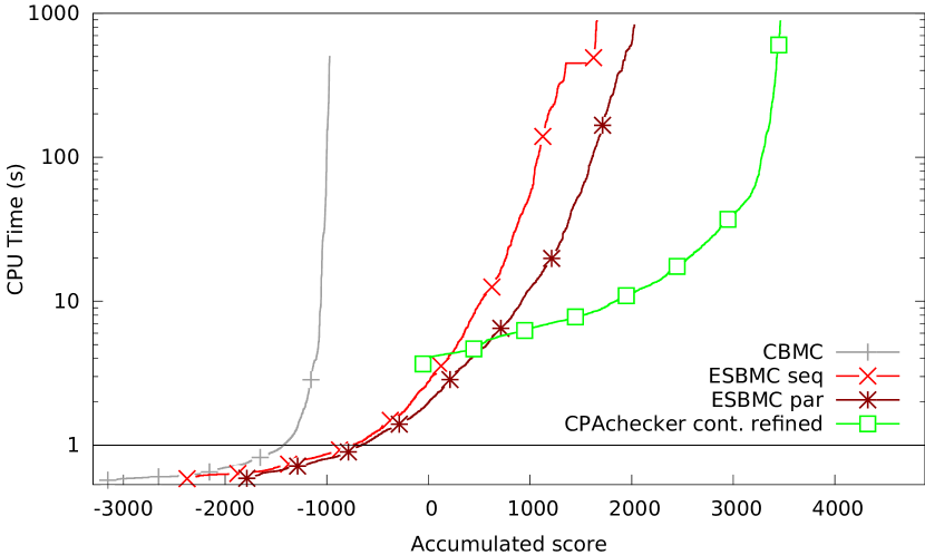
Figure 3: Quantile functions of $k$-induction-based tools for accumulated scores showing the CPU time for the successful results; linear scale between 0 s and 1 s, logarithmic scale beyond

Score. Both configurations of Esbmc produce a significant number of wrong results. All tools do produce some wrong answers, which are probably related to unsoundness and imprecision in the handling of some C features. CPAchecker with $k$-induction and sound invariants has only 1 missed bug (i.e, wrong claim of safety), whereas Esbmc, in the sequential version, has 184 wrong safety proofs. This large number of wrong results must be attributed to the unsound heuristic of Esbmc for strengthening the induction hypothesis, where it retains potentially incorrect information about loop-modified variables. The large number of wrong proofs reduces the confidence in the soundness of the correct proofs. Consequently, the score achieved by CPAchecker with continuously-refined invariants is much higher than the score of Esbmc (3 464 instead of 2 027 points). This clear advantage is also visible in Fig. 3.

When comparing the results of Esbmc to CPAchecker with a reimplemention of the unsound heuristic of Esbmc, we see that Esbmc produces fewer wrong results. The reason for this difference is that the heuristic only works well if relevant variables are identified on loop-exit conditions. Due to CPAchecker’s encoding of multiple loops in a program into a single loop for $k$-induction, the number of loop-exit conditions is smaller than in the original program, and the heuristic performs worse. However, even with the implementation in Esbmc, this unsound heuristic produces so many wrong results that it is not suited for verifying program safety.

The parallel version of Esbmc performs somewhat better than its sequential version, and misses fewer bugs. This is due to the fact that the base case and the step case are performed in parallel, and the loop bound $k$ is incremented independently for each of them. The base case is usually easier to solve for the SMT solver, and thus the base-case checks proceed faster than the step-case checks (reaching a higher value of $k$ sooner). Therefore, the parallel version manages to find some bugs by reaching the relevant $k$ in the base-case checks earlier than in the step-case checks, which would produce a wrong safety proof at reaching $k$. However, the number of wrong proofs is still much higher than with our approach, which is conceptually sound. Thus, our score is more than 1 400 points higher.

Performance. Table II shows that, if only the times for correct results are considered, our approach is considerably faster than Esbmc (Cbmc has so few correct results that the time for them is even less). This indicates that due to our invariants, we succeed more often with fewer loop unrollings and thus in less time. It also shows that the effort invested for generating the invariants is well spent. If considering the total time for the analysis of all results, CPAchecker needs more time. This is due to the fact that these measurements are dominated by those programs for which the tool runs into a timeout, and CPAchecker has more timeouts, whereas Esbmc has more wrong results (for which less time is spent). A timeout is generally preferable to a wrong result, though.

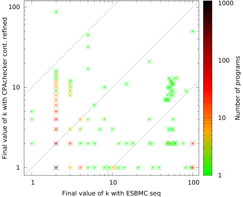
Figure 4: Scatter plot of the final value of $k$ for all safe programs verified successfully by both CPAchecker (continuously-refined invariants) and Esbmc (sequential) with $k$-induction; the color of each data point indicates the number of programs solved with this value of $k$

Final value of $k$. The bottom of Table II contains some statistics on the final value of $k$ that was needed to verify a program. Figure 4 shows a scatter plot comparing the values of the loop bound $k$ for CPAchecker with continuously-refined invariants and Esbmc in its sequential version. Both axes and the color range have a logarithmic scale. Data points are shown only for those $1\,460$ verification tasks that can be proved safe by both configurations. A point in the lower right half means that CPAchecker needed a lower $k$ (fewer loop unrollings) than Esbmc for the same verification task. The color of each data point gives an indication of how many verification tasks are represented by the data point. For example, the dark point at $(2,1)$ signifies that there are $845$ programs that can be verified by CPAchecker with a final value of $k=1$, whereas Esbmc needs $k=2$ for these programs.

The table shows that for safe programs, CPAchecker only needs a loop bound that is (on average) less than a third of the loop bound that Esbmc needs. The bottom of the plot shows that there are many programs (including the $845$ programs at $(2,1)$) that CPAchecker verifies with only one loop unrolling, but for which Esbmc needs to unroll the loops more often. To the right of the plot, there is also a group of programs for which Esbmc needs a $k$ between $45$ and $65$ to verify the program, and CPAchecker succeeds with significantly smaller $k$. There are only four programs for which CPAchecker needs a $k$ larger than $32$ (one program for $k=40$, $k=45$, $k=50$, and $k=88$ each). For Esbmc, the largest number of loop unrollings is $100$, which is necessary for $71$ programs. These advantages are due to the use of generated invariants, which make the induction proofs easier and likely to succeed with a smaller number of $k$. There is also a group of programs where Esbmc succeeds with $2$ loop unrollings but CPAchecker needs up to $16$. However, the number of such programs is relatively small (note that the data points with a green-to-orange color only represent $1$ to $9$ programs) and there is only a single program where CPAchecker unrolls the loops more than $10$ times more than Esbmc (while there are many with the reverse being true). The reason why Esbmc needs fewer loop unrollings for some programs is its (unsound) heuristic of keeping information about some program variables from the initial program state in the inductive-step case.

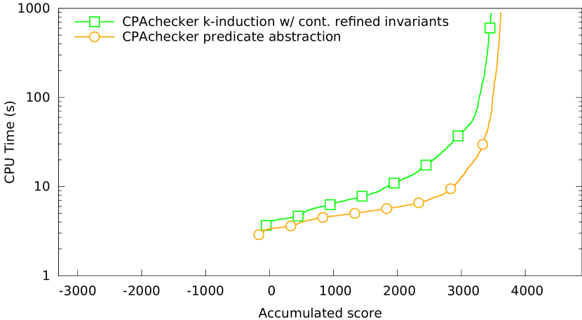
Figure 5: Quantile functions for accumulated scores showing the CPU time for the successful results

IV-F Comparison with other approaches

We also compare with the predicate-abstraction implementation of CPAchecker [11], which uses the same framework (parser, formula encoding, etc.) and SMT solver as our implementation of $k$-induction. The score-based quantile functions for our $k$-induction approach and the existing predicate abstraction in Fig. 5 show that the latter is somewhat faster and achieves a higher score. It is surprising that even the well-tuned CPAchecker implementation of the mature predicate-abstraction approach only slightly outperforms our novel $k$-induction implementation. The difference in performance and score between these two configurations is much smaller than the improvement of our approach compared to existing $k$-induction-based approaches (cf. Fig. 3). This is a promising result, considering that there is room for improvement in our approach. Especially the invariant generation could be further enhanced, e.g., by tailoring the invariant generation to the special needs of the $k$-induction proof, and a more targeted invariant-refinement procedure.

IV-G Acknowledgments

We would like to thank M. Tautschnig and L. Cordeiro for explaining the optimal available configuration for $k$-induction, for the verifiers Cbmc and Esbmc, respectively.

V Conclusion

We have presented the novel idea of combining $k$-induction with continuously-refined invariants, and contribute a publicly available implementation of our idea within the software-verification framework CPAchecker. Our extensive experiments show that our approach outperforms all existing implementations of $k$-induction for software verification, and that it is competitive compared to other, more mature techniques for software verification. We showed that a sound, effective, and efficient $k$-induction approach to general purpose software verification is possible, and that the additional resources required to achieve these combined benefits are negligible if invested judiciously. At the same time, there is still room for improvement of our technique. In the future, we plan to integrate successful features of other approaches to $k$-induction such as the parallel algorithm of Esbmc. The experiments with Esbmc show that we can avoid more timeouts on unsafe programs by running the iteratively-deepening BMC decoupled from the slower inductive-step case. We are also interested in adding an information flow between the two cooperating algorithms in the reverse direction. If the $k$-induction procedure could tell the invariant generation which facts it misses to prove safety, this could lead to a more efficient and effective approach that generates invariants that are specifically tailored to the needs of the $k$-induction proof. Already now, CPAchecker is parsimonious in terms of unrollings, compared to other tools. The low $k$-values required to prove many programs show that even our current invariant generation is powerful enough to produce invariants that are strong enough to help cut down the necessary number of loop unrollings. $k$-induction-guided precision refinement might direct the invariant generation towards providing weaker but still useful invariants for $k$-induction more efficiently.

References

- [1] A. V. Aho, R. Sethi, and J. D. Ullman. Compilers: Principles, Techniques, and Tools. Addison-Wesley, 1986.
- [2] M. Awedh and F. Somenzi. Automatic invariant strengthening to prove properties in bounded model checking. In Proc. DAC, pages 1073–1076. ACM/IEEE, 2006.
- [3] T. Ball, B. Cook, V. Levin, and S. Rajamani. SLAM and Static Driver Verifier: Technology transfer of formal methods inside Microsoft. In Proc. IFM, LNCS 2999, pages 1–20. Springer, 2004.
- [4] M. Barnett and K. R. M. Leino. Weakest-precondition of unstructured programs. In Proc. PASTE, pages 82–87. ACM, 2005.
- [5] D. Beyer. Second competition on software verification (summary of SV-COMP 2013). In Proc. TACAS, LNCS 7795, pages 594–609. Springer, 2013.
- [6] D. Beyer. Status report on software verification (competition summary SV-COMP 2014). In Proc. TACAS, LNCS 8413, pages 373–388. Springer, 2014.
- [7] D. Beyer, T. A. Henzinger, R. Majumdar, and A. Rybalchenko. Invariant synthesis for combined theories. In Proc. VMCAI, LNCS 4349, pages 378–394. Springer, 2007.
- [8] D. Beyer, T. A. Henzinger, and G. Théoduloz. Configurable software verification: Concretizing the convergence of model checking and program analysis. In Proc. CAV, LNCS 4590, pages 504–518. Springer, 2007.
- [9] D. Beyer, T. A. Henzinger, and G. Théoduloz. Program analysis with dynamic precision adjustment. In Proc. ASE, pages 29–38. IEEE, 2008.
- [10] D. Beyer and M. E. Keremoglu. CPAchecker: A tool for configurable software verification. In Proc. CAV, LNCS 6806, pages 184–190. Springer, 2011.
- [11] D. Beyer, M. E. Keremoglu, and P. Wendler. Predicate abstraction with adjustable-block encoding. In Proc. FMCAD, pages 189–197. FMCAD, 2010.
- [12] A. Biere. Handbook of Satisfiability. IOS Press, 2009.
- [13] A. Biere, A. Cimatti, E. M. Clarke, O. Strichman, and Y. Zhu. Bounded model checking. Advances in Computers, 58:117–148, 2003.
- [14] A. Biere, A. Cimatti, E. M. Clarke, and Y. Zhu. Symbolic model checking without BDDs. In Proc. TACAS, LNCS 1579, pages 193–207. Springer, 1999.
- [15] N. Bjørner, A. Browne, and Z. Manna. Automatic generation of invariants and intermediate assertions. Theor. Comput. Sci., 173(1):49–87, 1997.
- [16] A. R. Bradley and Z. Manna. Property-directed incremental invariant generation. FAC, 20(4-5):379–405, 2008.
- [17] L. Cordeiro, B. Fischer, and J. P. M. Silva. SMT-based bounded model checking for embedded ANSI-C software. In Proc. ASE, pages 137–148. IEEE, 2009.
- [18] A. F. Donaldson, L. Haller, and D. Kröning. Strengthening induction-based race checking with lightweight static analysis. In Proc. VMCAI, LNCS 6538, pages 169–183. Springer, 2011.
- [19] A. F. Donaldson, L. Haller, D. Kröning, and P. Rümmer. Software verification using k-induction. In Proc. SAS, LNCS 6887, pages 351–368. Springer, 2011.
- [20] A. F. Donaldson, D. Kröning, and P. Rümmer. Automatic analysis of scratch-pad memory code for heterogeneous multicore processors. In Proc. TACAS, LNCS 6015, pages 280–295. Springer, 2010.
- [21] A. F. Donaldson, D. Kröning, and P. Rümmer. Automatic analysis of DMA races using model checking and k-induction. FMSD, 39(1):83–113, 2011.
- [22] P. Garoche, T. Kahsai, and C. Tinelli. Incremental invariant generation using logic-based automatic abstract transformers. In Proc. NASA Formal Methods, LNCS 7871, pages 139–154. Springer, 2013.
- [23] D. Große, H. M. Le, and R. Drechsler. Proving transaction and system-level properties of untimed SystemC TLM designs. In Proc. MEMOCODE, pages 113–122. IEEE, 2010.
- [24] A. Gupta and A. Rybalchenko. Invgen: An efficient invariant generator. In Proc. CAV, LNCS 5643, pages 634–640. Springer, 2009.
- [25] A. Gurfinkel, A. Albarghouthi, S. Chaki, Y. Li, and M. Chechik. UFO: Verification with interpolants and abstract interpretation (competition contribution). In Proc. TACAS, pages 637–640. Springer, 2013.
- [26] T. Kahsai and C. Tinelli. Pkind: A parallel k-induction based model checker. In Proc. Int. Workshop on Parallel and Distributed Methods in Verification, EPTCS 72, pages 55–62, 2011.
- [27] A. V. Khoroshilov, V. Mutilin, A. Petrenko, and V. Zakharov. Establishing Linux driver verification process. In Proc. Ershov Memorial Conference, LNCS 5947, pages 165–176. Springer, 2009.
- [28] Z. Manna and A. Pnueli. Temporal Verification of Reactive Systems: Safety. Springer, 1995.
- [29] J. Morse, L. Cordeiro, D. Nicole, and B. Fischer. Handling unbounded loops with ESBMC 1.20 (competition contribution). In Proc. TACAS, LNCS 7795, pages 619–622. Springer, 2013.
- [30] M. Sheeran, S. Singh, and G. Stålmarck. Checking safety properties using induction and a SAT-solver. In Proc. FMCAD, LNCS 1954, pages 127–144. Springer, 2000.
- [31] T. Wahl. The k-induction principle, 2013. Available at http://www.ccs.neu.edu/home/wahl/Publications/k-induction.pdf.