Phenomenology of renormalons and the OPE from lattice regularization: the gluon condensate and the heavy quark pole mass

Abstract

We study the operator product expansion of the plaquette (gluon condensate) and the self-energy of an infinitely heavy quark. We first compute their perturbative expansions to order $\alpha^{35}$ and $\alpha^{20}$, respectively, in the lattice scheme. In both cases we reach the asymptotic regime where the renormalon behavior sets in. Subtracting the perturbative series, we obtain the leading non-perturbative corrections of their respective operator product expansions. In the first case we obtain the gluon condensate and in the second the binding energy of the heavy quark in the infinite mass limit. The results are fully consistent with the expectations from renormalons and the operator product expansion.

1 Introduction

The operator product expansion (OPE) Wilson:1969zs is a fundamental tool for theoretical analyses in quantum field theories. Its validity is only proven rigorously within perturbation theory, to arbitrary finite orders Zimmermann:1972tv . The use of the OPE in a non-perturbative framework was initiated by the ITEP group Vainshtein:1978wd (see also the discussion in Ref. Novikov:1984rf ), who postulated that the OPE of a correlator could be approximated by the following series:

$$\mathrm{correlator}(Q)\simeq\sum_{d}\frac{1}{Q^{d}}C_{d}(\alpha)\langle O_{d}\rangle\,,$$ (1)

where the expectation values of local operators $O_{d}$ are suppressed by inverse powers of a large external momentum $Q\gg\Lambda_{\mathrm{QCD}}$, according to their dimensionality $d$. The Wilson coefficients $C_{d}(\alpha)$ encode the physics at momentum scales larger than $Q$. These are well approximated by perturbative expansions in the strong coupling parameter $\alpha$:

$$C_{d}(\alpha)\simeq\sum_{n\geq 0}c_{n}\alpha^{n+1}\,.$$ (2)

The large-distance physics is described by the matrix elements $\langle O_{d}\rangle$ that usually have to be determined non-perturbatively: $\langle O_{d}\rangle\sim\Lambda_{\mathrm{QCD}}^{d}$.

It can hardly be overemphasized that (except for direct predictions of non-perturbative lattice simulations, e.g., on light hadron masses) all QCD predictions are based on factorizations that are generalizations of the above generic OPE.

There exist some major questions related to the OPE that have to be addressed:

• Are the perturbative expansions of Wilson coefficients asymptotic series?

• If so: are the associated ambiguities of the asymptotic behavior consistent with the OPE, i.e. with the positions of the expected renormalons Hooft in the Borel plane?

• Is the OPE valid beyond perturbation theory?

• What is the real size of the first non-perturbative correction within a given OPE expansion?

• Is this value strongly affected by ambiguities associated to renormalons?

In this paper we summarize and discuss our recent results Bauer:2011ws ; Bali:2013pla ; Bali:2013qla ; Bali:2014fea ; Bali:2014sja , which address these questions for the case of the plaquette and the energy of an infinitely heavy quark in the pure gluodynamics approximation to QCD. Both analyses utilize lattice regularization. Contrary to, e.g., dimensional regulation, lattice regularization can be defined non-perturbatively. Using a lattice scheme rather than the $\overline{\mathrm{MS}}$ scheme, we can, not only expand observables in perturbation theory, but also evaluate them non-perturbatively. Another advantage of this choice is that it enables us to use numerical stochastic perturbation theory DRMMOLatt94 ; DRMMO94 ; DR0 to obtain perturbative expansion coefficients. This allows us to realize much higher orders than would have been possible with diagrammatic techniques. A disadvantage of the lattice scheme is that, at least in our discretization, lattice perturbative expansions converge slower than expansions in the $\overline{\mathrm{MS}}$ coupling. This means that we have to go to comparatively higher orders to become sensitive to the asymptotic behavior. Many of the results obtained in a lattice scheme either directly apply to the $\overline{\mathrm{MS}}$ scheme too or can subsequently easily (and in some cases exactly) be converted into this scheme.

In our studies we used the Wilson gauge action Wilson:1974sk . We define the vacuum expectation value of a generic operator $B$ of engineering dimension zero as

$$\langle B\rangle\equiv\langle\Omega|B|\Omega\rangle=\frac{1}{Z}\int\![dU_{x,\mu}]\,e^{-S[U]}B[U]$$ (3)

with the partition function $Z=\int[dU_{x,\mu}]\,e^{-S[U]}$ and measure $[dU_{x,\mu}]=\prod_{x\in\Lambda_{E},\mu}dU_{x,\mu}$. $|\Omega\rangle$ denotes the vacuum state, $\Lambda_{E}$ is a Euclidean spacetime lattice with lattice spacing $a$ and $U_{x,\mu}\approx e^{iA_{\mu}(x+a/2)}\in\mathrm{SU}(3)$ is a gauge link.

2 The Plaquette: OPE in perturbation theory

For the case of the plaquette we have $B\rightarrow P$, where

$$\langle P\rangle=\frac{1}{N^{4}}\sum_{x\in\Lambda_{E}}\langle P_{x}\rangle\,,\quad P_{x}=1-\frac{1}{36}\sum_{\mu>\nu}\mathrm{Tr}\left(U_{x,\mu\nu}+U_{x,\mu\nu}^{\dagger}\right)\,,$$ (4)

and $U_{x,\mu\nu}$ denotes the oriented product of gauge links enclosing an elementary square (plaquette) in the $\mu$-$\nu$ plane of the lattice. For details on the notation and simulation set-up see Ref. Bali:2014fea .

$\langle P\rangle$ will depend on the lattice extent $Na$, the spacing $a$ and $\alpha=g^{2}/(4\pi)\equiv\alpha(a^{-1})$ (note that $\alpha$ is the bare lattice coupling and its natural scale is of order $a^{-1}$). We first compute this expectation value in strict perturbation theory. In other words, we Taylor expand in powers of $g$ before averaging over the gauge configurations (which we do using NSPT DRMMOLatt94 ; DRMMO94 ; DR0 ). The outcome is a power series in $\alpha$:

$$\langle P\rangle_{\mathrm{pert}}(N)\equiv\frac{1}{Z}\left.\int\![dU_{x,\mu}]\,e^{-S[U]}P[U]\right|_{\mathrm{NSPT}}=\sum_{n\geq 0}p_{n}(N)\alpha^{n+1}\,.$$

The dimensionless coefficients $p_{n}(N)$ are functions of the linear lattice size $N$. We emphasize that they do not depend on the lattice spacing $a$ or on the physical lattice extent $Na$ alone but only on the ratio $N=(Na)/a$.

We are interested in the large-$N$ (i.e. infinite volume) limit. In this situation

$$\frac{1}{a}\gg\frac{1}{Na}$$ (5)

and it makes sense to factorize the contributions of the different scales within the OPE framework. The hard modes, of scale $\sim 1/a$, determine the Wilson coefficients, whereas the soft modes, of scale $\sim 1/(Na)$, can be described by expectation values of local gauge invariant operators. There are no such operators of dimension two. The renormalization group invariant definition of the gluon condensate

$$\langle G^{2}\rangle=-\frac{2}{\beta_{0}}\left\langle\Omega\left|\frac{\beta(\alpha)}{\alpha}G_{\mu\nu}^{c}G_{\mu\nu}^{c}\right|\Omega\right\rangle=\left\langle\Omega\left|\left[1+\mathcal{O}(\alpha)\right]\frac{\alpha}{\pi}G_{\mu\nu}^{c}G_{\mu\nu}^{c}\right|\Omega\right\rangle$$ (6)

is the only local gauge invariant expectation value of an operator of dimension $a^{-4}$ in pure gluodynamics. In the purely perturbative case discussed here, this only depends on the soft scale $1/(Na)$, i.e. on the lattice extent. On dimensional grounds, the perturbative gluon condensate $\langle G^{2}\rangle_{\mathrm{soft}}$ is proportional to $1/(Na)^{4}$, and the logarithmic $(Na)$-dependence is encoded in $\alpha[1/(Na)]$. Therefore,

$$\frac{\pi^{2}}{36}\,a^{4}\langle G^{2}\rangle_{\mathrm{soft}}=-\frac{1}{N^{4}}\sum_{n\geq 0}f_{n}\alpha^{n+1}\![1/(Na)]\,,$$ (7)

and the perturbative expansion of the plaquette on a finite volume of $N^{4}$ sites can be written as

$$\langle P\rangle_{\mathrm{pert}}(N)=P_{\mathrm{pert}}(\alpha)\langle 1\rangle+\frac{\pi^{2}}{36}C_{\mathrm{G}}(\alpha)\,a^{4}\langle G^{2}\rangle_{\mathrm{soft}}+\mathcal{O}\left(\frac{1}{N^{6}}\right)\,,$$ (8)

where

$$P_{\mathrm{pert}}(\alpha)=\sum_{n\geq 0}p_{n}\alpha^{n+1}$$ (9)

and $p_{n}$ are the infinite volume coefficients that we are interested in. The constant pre-factor $\pi^{2}/36$ is chosen such that the Wilson coefficient, which only depends on $\alpha$, is normalized to unity for $\alpha=0$. It can be expanded in $\alpha$:

$$C_{\mathrm{G}}(\alpha)=1+\sum_{k\geq 0}c_{k}\alpha^{k+1}\,.$$ (10)

Since our action is proportional to the plaquette $P$, $C_{\mathrm{G}}$ is fixed by the conformal trace anomaly DiGiacomo:1990gy ; DiGiacomo:1989id :

$$C^{-1}_{\mathrm{G}}(\alpha)=-\frac{2\pi\beta(\alpha)}{\beta_{0}\alpha^{2}}=1+\frac{\beta_{1}}{\beta_{0}}\frac{\alpha}{4\pi}+\frac{\beta_{2}}{\beta_{0}}\left(\frac{\alpha}{4\pi}\right)^{2}+\frac{\beta_{3}}{\beta_{0}}\left(\frac{\alpha}{4\pi}\right)^{3}+\mathcal{O}(\alpha^{4})\,.$$ (11)

The $\beta$-function coefficients $\beta_{j}$ are known in the lattice scheme for $j\leq 3$ (see Eq. (25) of Ref. Bali:2014fea ).

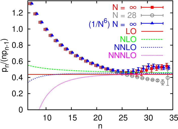
Figure 1: The ratios $p_{n}/(np_{n-1})$ compared with the leading order (LO), next-to-leading order (NLO), NNLO and NNNLO predictions of the $1/n$-expansion Eq. (14). Only the “$N=\infty$” extrapolation includes the systematic uncertainties. We also show finite volume data for $N=28$, and the result from the alternative $N\rightarrow\infty$ extrapolation including some $1/N^{6}$ corrections. The symbols have been shifted slightly horizontally.

Combining Eqs. (7), (8) and (10) gives

$$\langle P\rangle_{\mathrm{pert}}(N) =\sum_{n\geq 0}\left[p_{n}-\frac{f_{n}(N)}{N^{4}}\right]\alpha^{n+1}$$ (12)

$$=\sum_{n\geq 0}p_{n}\alpha^{n+1}-\frac{1}{N^{4}}\left(1+\sum_{k\geq 0}c_{k}\alpha^{k+1}(a^{-1})\right)\times\sum_{n\geq 0}f_{n}\alpha^{n+1}((Na)^{-1})+\mathcal{O}\left(\frac{1}{N^{6}}\right)\,,$$

where $f_{n}(N)$ is a polynomial in powers of $\ln(N)$. Fitting this equation to the perturbative lattice results, the first 35 coefficients $p_{n}$ were determined in Ref. Bali:2014fea . The results were confronted with the expectations from renormalons:

$$p^{\mathrm{latt}}_{n}\stackrel{{\scriptstyle n\rightarrow\infty}}{{=}}N^{\mathrm{latt}}_{P}\,\left(\frac{\beta_{0}}{2\pi d}\right)^{\!n}\frac{\Gamma(n+1+db)}{\Gamma(1+db)}\left[1+\frac{20.08931\ldots}{n+db}+\frac{505\pm 33}{\left(n+db\right)\left(n+db-1\right)}+\mathcal{O}\left(\frac{1}{n^{3}}\right)\right]\,,$$ (13)

$$\frac{p_{n}}{np_{n-1}}=\frac{\beta_{0}}{2\pi d}\left\{1+\frac{db}{n}+\frac{db(1-ds_{1})}{n^{2}}+\frac{db\left[1-3ds_{1}+d^{2}b(s_{1}+2s_{2})\right]}{n^{3}}+\mathcal{O}\left(\frac{1}{n^{4}}\right)\right\}\,,$$ (14)

where $b=\beta_{1}/(2\beta_{0}^{2})$, $s_{1}=(\beta_{1}^{2}-\beta_{0}\beta_{2})/(4b\beta_{0}^{4})$ and $s_{2}=(\beta_{1}^{3}-2\beta_{0}\beta_{1}\beta_{2}+\beta_{0}^{2}\beta_{3})/(16b^{2}\beta_{0}^{6})$ are defined so that

$$a=\frac{1}{\Lambda_{\mathrm{latt}}}\exp\left[-\frac{1}{t}-b\ln\frac{t}{2}+s_{1}bt-s_{2}b^{2}t^{2}+\cdots\right]\quad\mathrm{with}\quad t=\frac{\beta_{0}}{2\pi}\alpha\,.$$ (15)

In Fig. 1 we compare the infinite volume ratios $p_{n}/(np_{n-1})$ to the expectation Eq. (14): the asymptotic behavior of the perturbative series due to renormalons is reached around orders $n\sim 27-30$, proving, for the first time, the existence of the renormalon in the plaquette. Note that incorporating finite volume effects is compulsory to see this behavior, since there are no infrared renormalons on a finite lattice. To parameterize finite size effects we made use of the purely perturbative OPE Eq. (8). The behavior seen in Fig. 1, although computed from perturbative expansion coefficients, goes beyond the purely perturbative OPE since it predicts the position of a non-perturbative object in the Borel plane.

3 The plaquette: OPE beyond perturbation theory

Since in NSPT we Taylor expand in powers of $g$ before averaging over the gauge variables, no mass gap is generated. In non-perturbative Monte-Carlo (MC) lattice simulations an additional scale, $\Lambda_{\mathrm{QCD}}\sim 1/a\,e^{-2\pi/(\beta_{0}\alpha)}$, is generated dynamically (see also Eq. (15)). However, we can always tune $N$ and $\alpha$ such that

$$\frac{1}{a}\gg\frac{1}{Na}\gg\Lambda_{\mathrm{QCD}}\,.$$ (16)

In this small-volume situation we encounter a double expansion in powers of $a/(Na)$ and $a\Lambda_{\mathrm{QCD}}$ [or, equivalently, $(Na)\Lambda_{\mathrm{QCD}}\times a/(Na)$]. The construction of the OPE is completely analogous to that of the previous section and we obtain

$$\langle P\rangle_{\mathrm{MC}}=\frac{1}{Z}\left.\int\![dU_{x,\mu}]\,e^{-S[U]}P[U]\right|_{\mathrm{MC}}=P_{\mathrm{pert}}(\alpha)\langle 1\rangle+\frac{\pi^{2}}{36}C_{\mathrm{G}}(\alpha)\,a^{4}\langle G^{2}\rangle_{\mathrm{MC}}+\mathcal{O}(a^{6})\,.$$ (17)

In the last equality we have factored out the hard scale $1/a$ from the scales $1/(Na)$ and $\Lambda_{\mathrm{QCD}}$, which are encoded in $\langle G^{2}\rangle_{\mathrm{MC}}$. Exploiting the right-most inequality of Eq. (16), we can expand $\langle G^{2}\rangle_{\mathrm{MC}}$ as follows:

$$\langle G^{2}\rangle_{\mathrm{MC}}=\langle G^{2}\rangle_{\rm soft}\left\{1+\mathcal{O}[\Lambda_{\mathrm{QCD}}^{2}(Na)^{2}]\right\}\,.$$ (18)

Hence, a non-perturbative small-volume simulation would yield the same expression as NSPT, up to non-perturbative corrections that can be made arbitrarily small by reducing $a$ and therefore $Na$, keeping $N$ fixed. In other words, $p_{n}^{\mathrm{NSPT}}(N)=p_{n}^{\mathrm{MC}}(N)$ up to non-perturbative corrections.

We can also consider the limit

$$\frac{1}{a}\gg\Lambda_{\mathrm{QCD}}\gg\frac{1}{Na}\,.$$ (19)

This is the standard situation realized in non-perturbative lattice simulations. Again the OPE can be constructed as in the previous section, Eq. (17) holds, and the $p_{n}$- and $c_{n}$-values are still the same. The difference is that now

$$\langle G^{2}\rangle_{\mathrm{MC}}=\langle G^{2}\rangle_{\mathrm{NP}}\left[1+\mathcal{O}\left(\frac{1}{\Lambda_{\mathrm{QCD}}^{2}(Na)^{2}}\right)\right]\,,$$ (20)

where $\langle G^{2}\rangle_{\mathrm{NP}}\sim\Lambda_{\mathrm{QCD}}^{4}$ is the so-called non-perturbative gluon condensate introduced in Ref. Vainshtein:1978wd . From now on we will call this quantity simply the “gluon condensate” $\langle G^{2}\rangle$. We are now in the position

• to determine the gluon condensate and

• to check the validity of the OPE (at low orders in the $a^{2}$ scale expansion) for the case of the plaquette.

In order to do so we proceed as follows. The perturbative series is divergent due to renormalons and other, sub-leading, instabilities. This makes any determination of $\langle G^{2}\rangle$ ambiguous, unless we define precisely how to truncate or how to approximate the perturbative series. A reasonable definition that is consistent with $\langle G^{2}\rangle\sim\Lambda_{\mathrm{QCD}}^{4}$ can only be given if the asymptotic behavior of the perturbative series is under control. This has only been achieved recently Bali:2014fea , where the perturbative expansion of the plaquette was computed up to $\mathcal{O}(\alpha^{35})$, see the previous section. The observed asymptotic behavior was in full compliance with renormalon expectations, with successive contributions starting to diverge for orders around $\alpha^{27}$–$\alpha^{30}$ within the range of couplings $\alpha$ typically employed in present-day lattice simulations.

Extracting the gluon condensate from the average plaquette was pioneered in Refs. Di Giacomo:1981wt ; Kripfganz:1981ri ; DiGiacomo:1981dp ; Ilgenfritz:1982yx and many attempts followed during the next decades, see, e.g., Refs. Alles:1993dn ; DiRenzo:1994sy ; Ji:1995fe ; DiRenzo:1995qc ; Burgio:1997hc ; Horsley:2001uy ; Rakow:2005yn ; Meurice:2006cr ; Lee:2010hd ; Horsley:2012ra . These suffered from insufficiently high perturbative orders and, in some cases, also finite volume effects. The failure to make contact to the asymptotic regime prevented a reliable lattice determination of $\langle G^{2}\rangle$. This problem was solved in Ref. Bali:2014sja , which we now summarize.

Truncating the infinite sum at the order of the minimal contribution provides one definition of the perturbative series. Varying the truncation order will result in changes of size $\Lambda_{\mathrm{QCD}}^{4}a^{4}$, where the dimension $d=4$ is fixed by that of the gluon condensate. We approximate the asymptotic series by the truncated sum

$$S_{P}(\alpha)\equiv S_{n_{0}}(\alpha)\,,\quad\mathrm{where}\quad S_{n}(\alpha)=\sum_{j=0}^{n}p_{j}\alpha^{j+1}\,.$$ (21)

$n_{0}\equiv n_{0}(\alpha)$ is the order for which $p_{n_{0}}\alpha^{{n_{0}}+1}$ is minimal. We then obtain the gluon condensate from the relation

$$\langle G^{2}\rangle=\frac{36C_{\mathrm{G}}^{-1}(\alpha)}{\pi^{2}a^{4}(\alpha)}\left[\langle P\rangle_{\mathrm{MC}}(\alpha)-S_{P}(\alpha)\right]+\mathcal{O}(a^{2}\Lambda_{\mathrm{QCD}}^{2})\,.$$ (22)

$C^{-1}_{\mathrm{G}}(\alpha)$ is proportional to the $\beta$-function, and the first few terms are known, see Eq. (11). The corrections to $C_{\mathrm{G}}=1$ are small. However, the $\mathcal{O}(\alpha^{2})$ and $\mathcal{O}(\alpha^{3})$ terms are of similar sizes. We will account for this uncertainty in our error budget.

Following Eq. (22), we subtract the truncated sum $S_{P}(\alpha)$ calculated from the coefficients $p_{n}$ of Ref. Bali:2014fea from the MC data on $\langle P\rangle_{\mathrm{MC}}(\alpha)$ of Ref. Boyd:1996bx in the range $\beta\in[5.8,6.65]$ ($\beta=6/g^{2}$), where $a(\beta)$ is given by the phenomenological parametrization of Ref. Necco:2001xg ($x=\beta-6$)

$$a=r_{0}\exp\left(-1.6804-1.7331x+0.7849x^{2}-0.4428x^{3}\right)\,,$$ (23)

where $r_{0}\approx 0.5\,$fm. This corresponds to $(a/r_{0})^{4}\in[3.1\times 10^{-5},5.5\times 10^{-3}]$, covering more than two orders of magnitude.

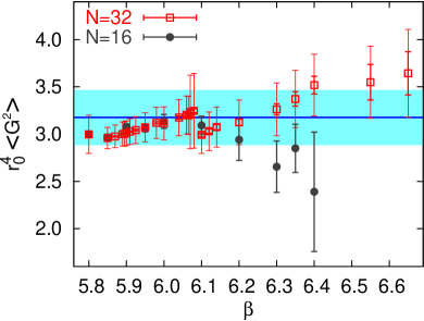
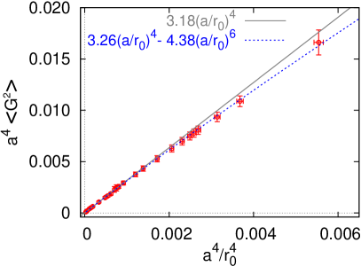
Figure 2: Left panel: Eq. (22) evaluated using the $N=16$ and $N=32$ MC data of Ref. Boyd:1996bx . The $N=32$ outer error bars include the error of $S_{P}(\alpha)$. The error band is our prediction for $\langle O_{G}\rangle$, Eq. (24).
Right panel: Eq. (22) times $a^{4}$ vs. $a^{4}(\alpha)/r_{0}^{4}$ from Eq. (23). The linear fit with slope Eq. (24) is to the $a^{4}<0.0013\,r_{0}^{4}$ points only.

Multiplying this difference by $36r_{0}^{4}/(\pi^{2}C_{\mathrm{G}}a^{4})$ gives $r_{0}^{4}\langle O_{\mathrm{G}}\rangle$ plus higher order non-perturbative terms. We show this combination in the left panel of Fig. 2. The smaller error bars represent the errors of the MC data, the outer error bars (not plotted for $N=16$) the total uncertainty, including that of $S_{P}$. This part of the error is correlated between different $\beta$-values (see the discussion in Ref Bali:2014sja ). The MC data were obtained on volumes $N^{4}=16^{4}$ and $N^{4}=32^{4}$. Towards large $\beta$-values the physical volumes $[Na(\beta)]^{4}$ will become small, resulting in transitions into the deconfined phase. For $\beta<6.3$ we find no significant differences between the $N=16$ and $N=32$ results. In the analysis we restrict ourselves to the more precise $N=32$ data and, to keep finite size effects under control, to $\beta\leq 6.65$. We also limit ourselves to $\beta\geq 5.8$ to avoid large $\mathcal{O}(a^{2})$ corrections. At very large $\beta$-values not only does the parametrization Eq. (23) break down but obtaining meaningful results becomes challenging numerically: the individual errors both of $\langle P\rangle_{\mathrm{MC}}(\alpha)$ and of $S_{P}(\alpha)$ somewhat decrease with increasing $\beta$. However, there are strong cancellations between these two terms, in particular at large $\beta$-values, since this difference decreases with $a^{-4}\sim\Lambda_{\mathrm{latt}}^{4}\exp(16\pi^{2}\beta/33)$ on dimensional grounds while $\langle P\rangle_{\mathrm{MC}}$ depends only logarithmically on $a$.

The data in the left panel of Fig. 2 show an approximately constant behavior. This indicates that, after subtracting $S_{P}(\alpha)$ from the corresponding MC values $\langle P\rangle_{\mathrm{MC}}(\alpha)$, the remainder scales like $a^{4}$. This can be seen more explicitly in the right panel of Fig. 2, where we plot this difference in lattice units against $a^{4}$. The result is consistent with a linear behavior but a small curvature seems to be present that can be parametrized as an $a^{6}$-correction. The right-most point ($\beta=5.8$) corresponds to $a^{-1}\simeq 1.45$ GeV while $\beta=6.65$ corresponds to $a^{-1}\simeq 5.3$ GeV. Note that $a^{2}$-terms are clearly ruled out.

We now determine the gluon condensate. We obtain the central value and its statistical error $\langle G^{2}\rangle=3.177(36)r_{0}^{-4}$ from averaging the $N=32$ data for $6.0\leq\beta\leq 6.65$. We now estimate the systematic uncertainties. Different infinite volume extrapolations of the $p_{n}(N)$ data Bali:2014fea result in changes of the prediction of about $6\%$. Another $6\%$ error is due to including an $a^{6}$-term or not and varying the fit range. Next there is a scale error of about 2.5%, translating $a^{4}$ into units of $r_{0}$. The uncertainty of the perturbatively determined Wilson coefficient $C_{\mathrm{G}}$ is of a similar size. This is estimated as the difference between evaluating Eq. (11) to $\mathcal{O}(\alpha^{2})$ and to $\mathcal{O}(\alpha^{3})$. Adding all these sources of uncertainty in quadrature and using the pure gluodynamics value Capitani:1998mq $\Lambda_{\overline{\mathrm{MS}}}=0.602(48)r_{0}^{-1}$ yields

$$\langle G^{2}\rangle=3.18(29)r_{0}^{-4}=24.2(8.0)\Lambda_{\overline{\mathrm{MS}}}^{4}\,.$$ (24)

The gluon condensate Eq. (6) is independent of the renormalization scale. However, $\langle G^{2}\rangle$ was obtained employing one particular prescription in terms of the observable and our choice of how to truncate the perturbative series within a given renormalization scheme. Different (reasonable) prescriptions can in principle give different results. One may for instance choose to truncate the sum at orders $n_{0}(\alpha)\pm\sqrt{n_{0}(\alpha)}$ and the result would still scale like $\Lambda_{\mathrm{QCD}}^{4}$. We estimated this intrinsic ambiguity of the definition of the gluon condensate in Ref. Bali:2014fea as $\delta\langle G^{2}\rangle=36/(\pi^{2}C_{\mathrm{G}}a^{4})\,\sqrt{n_{0}}p_{n_{0}}\alpha^{n_{0}+1}$, i.e. as $\sqrt{n_{0}(\alpha)}$ times the contribution of the minimal term:

$$\delta\langle G^{2}\rangle=27(11)\Lambda_{\overline{\mathrm{MS}}}^{4}\,.$$ (25)

Up to $1/n_{0}$-corrections this definition is scheme- and scale-independent and corresponds to the (ambiguous) imaginary part of the Borel integral times $\sqrt{2/\pi}$.

In QCD with sea quarks the OPE of the average plaquette or of the Adler function will receive additional contributions from the chiral condensate. For instance $\langle G^{2}\rangle$ needs to be redefined, adding terms $\propto\langle\gamma_{m}(\alpha)m\bar{\psi}\psi\rangle$ Tarrach:1981bi ; Bali:2013esa . Due to this and the problem of setting a physical scale in pure gluodynamics, it is difficult to assess the precise numerical impact of including sea quarks onto our estimates

$$\langle G^{2}\rangle\simeq 0.077\,\mathrm{GeV}^{4}\,,\quad\delta\langle G^{2}\rangle\simeq 0.087\,\mathrm{GeV}^{4}\,,$$ (26)

which we obtain using $r_{0}\simeq 0.5$ fm Sommer:1993ce . While the systematics of applying Eqs. (24)–(25) to full QCD are unknown, our main observations should still extend to this case. We remark that our prediction of the gluon condensate Eq. (26) is significantly bigger than values obtained in one- and two-loop sum rule analyses, ranging from 0.01 GeV⁴ Vainshtein:1978wd ; Ioffe:2002be up to 0.02 GeV⁴ Broadhurst:1994qj ; Narison:2011xe . However, these numbers were not extracted in the asymptotic regime, which for a $d=4$ renormalon in the $\overline{\mathrm{MS}}$ scheme we expect to set in at orders $n\gtrsim 7$. Moreover, we remark that in schemes without a hard ultraviolet cut-off, like dimensional regularization, the extraction of $\langle G^{2}\rangle$ can become obscured by the possibility of ultraviolet renormalons. Independent of these considerations, all these values are smaller than the intrinsic prescription dependence Eq. (25).

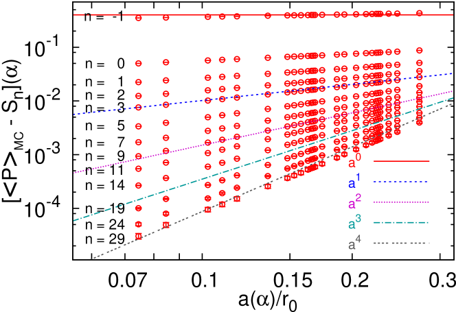
Figure 3: Differences $\langle P\rangle_{\mathrm{MC}}(\alpha)-S_{n}(\alpha)$ between MC data and sums truncated at orders $\alpha^{n+1}$ ($S_{-1}=0$) vs. $a(\alpha)/r_{0}$. The lines $\propto a^{j}$ are drawn to guide the eye.

Our analysis confirms the validity of the OPE beyond perturbation theory for the case of the plaquette. Our $a^{4}$-scaling clearly disfavors suggestions about the existence of dimension two condensates beyond the standard OPE framework Burgio:1997hc ; Chetyrkin:1998yr ; Gubarev:2000nz ; RuizArriola:2006gq ; Andreev:2006vy . In fact we can also explain why an $a^{2}$-contribution to the plaquette was found in Ref. Burgio:1997hc . In the log-log plot of Fig. 3 we subtract sums $S_{n}$, truncated at different fixed orders $\alpha^{n+1}$, from $\langle P\rangle_{\mathrm{MC}}$. The scaling continuously moves from $\sim a^{0}$ at $\mathcal{O}(\alpha^{0})$ to $\sim a^{4}$ around $\mathcal{O}(\alpha^{30})$. Note that truncating at an $\alpha$-independent fixed order is inconsistent, explaining why in the figure we never exactly obtain an $a^{4}$-slope. For $n\sim 9$ we reproduce the $a^{2}$-scaling reported in Ref. Burgio:1997hc for a fixed order truncation at $n=7$. In view of Fig. 3, we conclude that the observation of this scaling power was accidental.

4 The binding energy of HQET: OPE in perturbation theory

The OPE of the plaquette is analogous to the OPE of the vacuum polarization (or the Adler function) in position space. As we already mentioned, the OPE concept of the factorization of scales can also be applied to more general kinematical settings (in particular to cases where some scales are defined in Minkowski spacetime). A prominent example is heavy quark effective theory (HQET). In this case the term $\langle O_{1}\rangle$ of Eq. (1) is replaced by a non-perturbative quantity, the so-called heavy quark binding energy $\overline{\Lambda}$, that cannot be represented as an expectation value of a local gauge invariant operator. We consider the self-energy of a heavy quark in the infinite mass limit (in other words, the self-energy of a static source in the triplet representation, for other color representations see Ref. Bali:2013pla ), that is closely related to $\overline{\Lambda}$. We compute this quantity in close analogy to the case of the plaquette in lattice regularization.

First we compute the self-energy of the static quark in perturbation theory (again using NSPT). We obtain this from the Polyakov loop in an asymmetric volume $N_{S}^{3}N_{T}a^{4}$ of spatial and temporal extents $N_{S}a$ and $N_{T}a$, respectively:

$$L(N_{S},N_{T})=\frac{1}{N_{S}^{3}}\sum_{\mathbf{x}}\frac{1}{3}\mathrm{Tr}\left[\prod_{x_{4}/a=0}^{N_{T}-1}U_{x,4}\right]\,,$$ (27)

or, more specifically, from its logarithm

$$P(N_{S},N_{T})=-\frac{\ln\langle L(N_{S},N_{T})\rangle_{\mathrm{pert}}}{aN_{T}}=\sum_{n\geq 0}c_{n}(N_{S},N_{T})\alpha^{n+1}\,.$$ (28)

Again, $U_{x,\mu}$ denotes a gauge link and $x=(\mathbf{x},x_{4})\in\Lambda_{E}$ are Euclidean lattice points. We define the energy of a static source and its perturbative expansion in a finite spatial volume,

$$\delta m(N_{S})=\lim_{N_{T}\rightarrow\infty}P(N_{S},N_{T})=\frac{1}{a}\sum_{n\geq 0}c_{n}(N_{S})\alpha^{n+1}\!(1/a)\,,\quad\mathrm{where}\quad c_{n}(N_{S})=\lim_{N_{T}\rightarrow\infty}c_{n}(N_{S},N_{T})\,,$$ (29)

and its infinite volume limit

$$\delta m=\lim_{N_{S},N_{T}\rightarrow\infty}P(N_{S},N_{T})=\frac{1}{a}\sum_{n=0}^{\infty}c_{n}\alpha^{n+1}\!(1/a)\quad\mathrm{with}\quad c_{n}=\lim_{N_{S}\rightarrow\infty}c_{n}(N_{S})\,.$$ (30)

We now construct the purely perturbative OPE in a finite volume. For large $N_{S}$, we can write [$a^{-1}\gg(N_{S}a)^{-1}$]:

$$\delta m(N_{S}) =\frac{1}{a}\sum_{n\geq 0}^{\infty}\left(c_{n}-\frac{f_{n}(N_{S})}{N_{S}}\right)\alpha^{n+1}\!(1/a)+\mathcal{O}{\left(\frac{1}{N_{S}^{2}}\right)}$$ (31)

$$=\frac{1}{a}\sum_{n\geq 0}c_{n}\alpha^{n+1}\!\!\left(1/a\right)-\frac{1}{N_{S}a}\sum_{n\geq 0}f_{n}\alpha^{n+1}\!\!\left[1/(N_{S}a)\right]+\mathcal{O}{\left(\frac{1}{N_{S}^{2}}\right)}\,.$$

Note the similarity between this equation and Eq. (12). $f_{n}(N_{S})=\sum_{j=0}^{n}f_{n}^{(j)}\ln^{j}(N_{S})$ is again a polynomial in powers of $\ln(N_{S})$, and the $f_{n}^{(j)}$ are known combinations of $\beta$-function coefficients and lower order infinite volume expansion coefficients $c_{k}$, $k<n$. The main difference with respect to the gluon condensate is that the power correction scales like $1/N_{S}$, instead of $1/N_{S}^{4}$, and that now the Wilson coefficient is trivial. This $1/N_{S}$ scaling also means that the renormalon behavior will show up at lower orders $n$ of the perturbative expansion. Fitting the $c_{n}(N_{S})$ data to this equation, the first 20 $c_{n}$ coefficients were determined in Refs. Bauer:2011ws ; Bali:2013pla ; Bali:2013qla and confronted with the renormalon expectations:

$$c_{n}\stackrel{{\scriptstyle n\rightarrow\infty}}{{=}}N_{m}\,\left(\frac{\beta_{0}}{2\pi}\right)^{n}\,\frac{\Gamma(n+1+b)}{\Gamma(1+b)}\left[1+\frac{bs_{1}}{(n+b)}+\frac{b^{2}\left(s_{1}^{2}/2-s_{2}\right)}{(n+b)(n+b-1)}+\cdots\right]\,.$$ (32)

In the lattice scheme the numerical values of the above coefficients read $bs_{1}=1.36095381(11)$ and $b^{2}(s_{1}^{2}/2-s_{2})=5.34(51)$. As expected, the above expansion converges much faster in $1/n$ than Eq. (13). Calculating the ratio of subsequent perturbative coefficients gives

$$\frac{c_{n}}{c_{n-1}}\frac{1}{n}=\frac{\beta_{0}}{2\pi}\left\{1+\frac{b}{n}-\frac{bs_{1}}{n^{2}}+\frac{1}{n^{3}}\left[2b^{2}s_{2}+b(b-1)s_{1}\right]+\mathcal{O}\left(\frac{1}{n^{4}}\right)\right\}\,.$$ (33)

We remark that Eq. (14) includes the effect of the non-trivial Wilson coefficient $C_{\mathrm{G}}$. Therefore, just setting $d=1$ in that equation does not result in Eq. (33) above.

In Fig. 4 we compare the data to Eq. (33) for two different lattice discretizations of the covariant temporal derivative, which amounts to “smearing” or not smearing temporal gauge links. This should not affect the infrared behavior and, indeed, beyond the first few orders the difference becomes invisible. The asymptotic behavior of the perturbative series due to the renormalon is confirmed in full glory for $n\gtrsim 8$, proving the existence of the renormalon behavior in QCD beyond any reasonable doubt. Again the incorporation of finite volume effects was decisive to obtain this result.

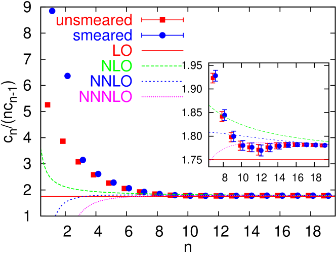
Figure 4: Ratios $c_{n}/(nc_{n-1})$ of the unsmeared (squares) and smeared (circles) triplet static self-energy coefficients $c_{n}$ in comparison to the theoretical prediction Eq. (33), truncated at different orders in $1/n$. In the inset we magnify the asymptotic region.

5 The binding energy of HQET: OPE beyond perturbation theory

The methods used for the gluon condensate can also be applied to other observables. We now consider the non-perturbative evaluation of the energy of a static-light meson on the lattice and its OPE:

$$E_{\mathrm{MC}}(\alpha)=E_{\mathrm{pert}}(\alpha)+\overline{\Lambda}+\mathcal{O}(a\Lambda_{\mathrm{QCD}}^{2})\,.$$ (34)

$\overline{\Lambda}$ is the non-perturbative binding energy and $E_{\mathrm{pert}}(\alpha)=\delta m(\alpha)$ is the self-energy of the static source in perturbation theory, i.e. Eq. (30). In HQET the mass of the $B$ meson is given as $m_{B}=m_{b,\mathrm{pert}}+\overline{\Lambda}+\mathcal{O}(1/m_{b})$, where $m_{b,\mathrm{pert}}$ is the $b$-quark pole mass $m_{b}^{\mathrm{OS}}$, which suffers from the same renormalon ambiguity as $\delta m$ Bigi:1994em ; Beneke:1994sw ; Neubert:1994wq .

The perturbative expansion of $a\delta m(\alpha)=\sum_{n}c_{n}\alpha^{n+1}$ was obtained in Refs. Bauer:2011ws ; Bali:2013pla up to $\mathcal{O}(\alpha^{20})$, see the previous section. Its intrinsic ambiguity

$$\delta\overline{\Lambda}=\sqrt{n_{0}}c_{n_{0}}\alpha^{n_{0}+1}=0.748(42)\Lambda_{\overline{\mathrm{MS}}}=0.450(44)r_{0}^{-1}$$ (35)

was computed in Refs. Bali:2013pla ; Bali:2013qla . MC data for the ground state energy $E_{\mathrm{MC}}$ of a static-light meson with the Wilson action can be found in Refs. Duncan:1994uq ; Allton:1994tt ; Ewing:1995ih .

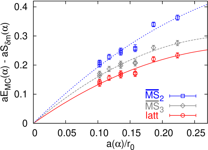
Figure 5: $a\overline{\Lambda}=aE_{\mathrm{MC}}-aS_{\delta m}$ vs. $a/r_{0}$. The sum $aS_{\delta m}$ Eq. (36) was also converted into the $\overline{\mathrm{MS}}$ scheme at two ($\overline{\mathrm{MS}}_{2}$) and three ($\overline{\mathrm{MS}}_{3}$) loops and truncated at the respective minimal orders. The curves are fits to $\overline{\Lambda}a+ca^{2}/r_{0}^{2}$.

Truncating the infinite sum in $\delta m$ at the order of the minimal contribution provides one definition of the perturbative series. As we did for the plaquette, we approximate the asymptotic series by the truncated sum

$$S_{\delta m}(\alpha)\equiv\frac{1}{a}\sum_{j=0}^{n_{0}(\alpha)}c_{j}\alpha^{j+1}\,,$$ (36)

where $n_{0}\equiv n_{0}(\alpha)$ is the order for which $c_{n_{0}}\alpha^{{n_{0}}+1}$ is minimal. While for the gluon condensate we expected an $a^{4}$-scaling (see the right panel of Fig. 2), for $a\overline{\Lambda}=aE_{\mathrm{MC}}-aS_{\delta m}(\alpha)$ we expect a scaling linear in $a$. Comforting enough this is what we find, up to the expected $a\mathcal{O}(a\Lambda_{\mathrm{QCD}}^{2})$ discretization corrections, see Fig. 5. Subtracting the partial sum truncated at orders $n_{0}(\alpha)=6$ from the $\beta\in[5.9,6.4]$ data, we obtain $\overline{\Lambda}=1.55(8)r_{0}^{-1}$ from such a linear plus quadratic fit, where we only give the statistical uncertainty. The errors of the perturbative coefficients are all tiny, which allows us to transform the expansion $a\delta m(\alpha)$ into $\overline{\mathrm{MS}}$-like schemes and to compute $\overline{\Lambda}$ accordingly. We define the schemes $\overline{\mathrm{MS}}_{2}$ and $\overline{\mathrm{MS}}_{3}$ by truncating $\alpha_{\overline{\mathrm{MS}}}(a^{-1})=\alpha(1+d_{1}\alpha+d_{2}\alpha^{2}+\ldots)$ exactly at $\mathcal{O}(\alpha^{3})$ and $\mathcal{O}(\alpha^{4})$, respectively. The $d_{j}$ are known for $j\leq 3$ Bali:2013pla ; Bali:2013qla . We typically find $n_{0}^{\overline{\mathrm{MS}}_{i}}(\alpha_{\overline{\mathrm{MS}}_{i}})=2,3$ and obtain $\overline{\Lambda}\sim 2.17(8)r_{0}^{-1}$ and $\overline{\Lambda}\sim 1.89(8)r_{0}^{-1}$, respectively, see Fig. 5. We conclude that the changes due to these resummations are indeed of the size $\delta\overline{\Lambda}\sim 0.5r_{0}^{-1}$, adding confidence that our definition of the ambiguity Eq. (35) is neither a gross overestimate nor an underestimate. For the plaquette, where we expect $n_{0}^{\overline{\mathrm{MS}}}\sim 7$, we cannot carry out a similar analysis, due to the extremely high precision that is required to resolve the differences between $S_{P}(\alpha)$ and $\langle P\rangle_{\mathrm{MC}}(\alpha)$, which largely cancel in Eq. (22).

6 Conclusions

For the first time ever, perturbative expansions at orders where the asymptotic regime is reached have been obtained and subtracted from non-perturbative Monte Carlo data of the static-light meson mass and of the plaquette, thereby validating the OPE for these cases beyond perturbation theory. The scaling of the latter difference with the lattice spacing confirms the dimension $d=4$. Dimension $d<4$ slopes appear only when subtracting the perturbative series truncated at fixed pre-asymptotic orders. Therefore, we interpret the lower dimensional “condensates” discussed in Ref. Chetyrkin:1998yr as approximate parametrizations of unaccounted perturbative effects, i.e. of the short-distance behavior. These will be observable-dependent, unlike the non-perturbative gluon condensate. Such simplified parametrizations introduce unquantifiable errors and, therefore, are of limited phenomenological use. As we have demonstrated above (see Fig. 3), even the effective dimension of such a “condensate” varies when truncating a perturbative series at different orders. In Refs. Gubarev:2000nz ; RuizArriola:2006gq ; Andreev:2006vy various analyses, based on models such as string/gauge duality or Regge models, have been made claiming the existence of non-perturbative dimension two condensates. Our results strongly suggest that there may be flaws in these derivations.

We observe that $\overline{\Lambda}$ and $\langle G^{2}\rangle$ do not depend on the lattice spacing (i.e. on the renormalization scale). In other words, they are renormalization group invariant quantities, as expected. This is coherent with the interpretation of these quantities to be of order $\Lambda_{\mathrm{QCD}}$ and $\Lambda_{\mathrm{QCD}}^{4}$, respectively. However, the values of $\overline{\Lambda}$ and $\langle G^{2}\rangle$ will depend on the details of how the divergent perturbative series is truncated or estimated (and therefore implicitly also on the scheme used in the perturbative expansion), as well as on the observable used as an input in the determination.

We have obtained an accurate value of the gluon condensate in SU(3) gluodynamics, Eq. (24). It is of a similar size as the intrinsic difference, Eq. (25), between (reasonable) subtraction prescriptions. This result contradicts the implicit assumption of sum rule analyses that the renormalon ambiguity is much smaller than leading non-perturbative corrections. The value of the gluon condensate obtained with sum rules can vary significantly due to this intrinsic ambiguity if determined using different prescriptions or truncating at different orders in perturbation theory. Clearly, the impact of this, e.g., on determinations of $\alpha_{s}$ from $\tau$-decays or from lattice simulations needs to be assessed carefully.

As already mentioned in the previous paragraph, due to the non-convergent nature of the perturbative series, the binding energy $\overline{\Lambda}$ and the gluon condensate $\langle G^{2}\rangle$ are in principle ill-defined quantities. The intrinsic ambiguity of their definition can, however, be estimated. The ambiguity of the HQET binding energy $\delta\overline{\Lambda}=0.75(4)\Lambda_{\overline{\mathrm{MS}}}$ as well as the ambiguity $\delta\langle G^{2}\rangle=27(11)\Lambda_{\overline{\mathrm{MS}}}^{4}$ of the non-perturbative gluon condensate are scale- and renormalization-scheme independent, at least up to $1/n_{0}$-corrections, where $n_{0}$ is the order of the minimal term of the perturbative series. In the first case this ambiguity is significantly smaller than $\overline{\Lambda}\simeq 2.6\Lambda_{\overline{\mathrm{MS}}}$. In the second case the ambiguity is larger than values typically quoted for $\langle G^{2}\rangle$, including our result $\langle G^{2}\rangle\simeq 24\Lambda_{\overline{\mathrm{MS}}}^{4}$. The size of $\delta\langle G^{2}\rangle\gtrsim\langle G^{2}\rangle$ means that, at least in pure gluodynamics, $\langle G^{2}\rangle$ should not be used to estimate the magnitude of unknown non-perturbative corrections. Instead, the ambiguity $\delta\langle G^{2}\rangle$ should be used for this purpose. An exception to this rule are situations where the renormalon ambiguities cancel exactly or are small. For instance, the perturbative expansion of a difference between two observables $\langle B_{2}\rangle-\langle B_{1}\rangle$ that receive contributions $\propto C_{B_{j}}\langle G^{2}\rangle/Q^{4}$ with a relative normalization such that $C_{B_{1}}=C_{B_{2}}+\mathcal{O}(\alpha)$ will be partially blind to the associated $d=4$ infrared renormalon if the $\langle B_{j}\rangle$ are expanded at the same scale, in the same renormalization scheme and the same method is used to truncate both perturbative series.

References

- (1) K. G. Wilson, Phys. Rev. 179, 1499 (1969).
- (2) W. Zimmermann, Annals Phys. 77, 570 (1973) [Lect. Notes Phys. 558, 278 (2000)].
- (3) A. I. Vainshtein, V. I. Zakharov and M. A. Shifman, JETP Lett. 27, 55 (1978) [Pi’sma Zh. Eksp. Teor. Fiz. 27, 60 (1978)].
- (4) V. A. Novikov, M. A. Shifman, A. I. Vainshtein and V. I. Zakharov, Nucl. Phys. B249, 445 (1985) [Yad. Fiz. 41, 1063 (1985)].
- (5) G. ’t Hooft, in Proceedings of the International School of Subnuclear Physics: The Whys of Subnuclear Physics, Erice 1977, edited by A. Zichichi, Subnucl. Ser. 15 (Plenum, New York, 1979) 943.
- (6) C. Bauer, G. S. Bali and A. Pineda, Phys. Rev. Lett. 108, 242002 (2012) [arXiv:1111.3946 [hep-ph]].
- (7) G. S. Bali, C. Bauer, A. Pineda and C. Torrero, Phys. Rev. D 87, 094517 (2013) [arXiv:1303.3279 [hep-lat]].
- (8) G. S. Bali, C. Bauer and A. Pineda, Proc. Sci. LATTICE 2013 (2014) 371 [arXiv:1311.0114 [hep-lat]].
- (9) G. S. Bali, C. Bauer and A. Pineda, Phys. Rev. D 89, 054505 (2014) [arXiv:1401.7999 [hep-ph]].
- (10) G. S. Bali, C. Bauer and A. Pineda, Phys. Rev. Lett. 113, 092001 (2014) [arXiv:1403.6477 [hep-ph]].
- (11) F. Di Renzo, G. Marchesini, P. Marenzoni and E. Onofri, Nucl. Phys. B Proc. Suppl. 34 (1994) 795.
- (12) F. Di Renzo, E. Onofri, G. Marchesini and P. Marenzoni, Nucl. Phys. B426, 675 (1994) [arXiv:hep-lat/9405019].
- (13) F. Di Renzo and L. Scorzato, J. High Energy Phys. 0410, 073 (2004) [arXiv:hep-lat/0410010].
- (14) K. G. Wilson, Phys. Rev. D 10, 2445 (1974).
- (15) A. Di Giacomo, H. Panagopoulos and E. Vicari, Phys. Lett. B 240, 423 (1990).
- (16) A. Di Giacomo, H. Panagopoulos and E. Vicari, Nucl. Phys. B338, 294 (1990).
- (17) A. Di Giacomo and G. C. Rossi, Phys. Lett. 100B, 481 (1981).
- (18) J. Kripfganz, Phys. Lett. 101B, 169 (1981).
- (19) A. Di Giacomo and G. Paffuti, Phys. Lett. 108B, 327 (1982).
- (20) E.-M. Ilgenfritz and M. Müller-Preußker, Phys. Lett. 119B, 395 (1982).
- (21) B. Alles, M. Campostrini, A. Feo and H. Panagopoulos, Phys. Lett. B 324, 433 (1994) [arXiv:hep-lat/9306001].
- (22) F. Di Renzo, E. Onofri, G. Marchesini and P. Marenzoni, Nucl. Phys. B426, 675 (1994) [arXiv:hep-lat/9405019].
- (23) X.-D. Ji, arXiv:hep-ph/9506413.
- (24) F. Di Renzo, E. Onofri and G. Marchesini, Nucl. Phys. B457, 202 (1995) [arXiv:hep-th/9502095].
- (25) G. Burgio, F. Di Renzo, G. Marchesini and E. Onofri, Phys. Lett. B422, 219 (1998) [arXiv:hep-ph/9706209].
- (26) R. Horsley, P. E. L. Rakow and G. Schierholz, Nucl. Phys. B Proc. Suppl. 106 (2002) 870 [arXiv:hep-lat/0110210].
- (27) P. E. L. Rakow, Proc. Sci. LAT2005 (2006) 284 [arXiv:hep-lat/0510046].
- (28) Y. Meurice, Phys. Rev. D 74, 096005 (2006) [arXiv:hep-lat/0609005].
- (29) T. Lee, Phys. Rev. D 82, 114021 (2010) [arXiv:1003.0231 [hep-ph]].
- (30) R. Horsley, G. Hotzel, E.-M. Ilgenfritz, R. Millo, H. Perlt, P. E. L. Rakow, Y. Nakamura, G. Schierholz and A. Schiller [QCDSF Collaboration], Phys. Rev. D 86, 054502 (2012) [arXiv:1205.1659 [hep-lat]].
- (31) G. Boyd, J. Engels, F. Karsch, E. Laermann, C. Legeland, M. Lütgemeier and B. Petersson, Nucl. Phys. B469, 419 (1996) [arXiv:hep-lat/9602007].
- (32) S. Necco and R. Sommer, Nucl. Phys. B622, 328 (2002) [arXiv:hep-lat/0108008].
- (33) S. Capitani, M. Łüscher, R. Sommer and H. Wittig [ALPHA Collaboration], Nucl. Phys. B544, 669 (1999) [arXiv:hep-lat/9810063].
- (34) R. Tarrach, Nucl. Phys. B196, 45 (1982).
- (35) G. S. Bali, F. Bruckmann, G. Endrődi, F. Gruber and A. Schäfer, JHEP 1304, 130 (2013) [arXiv:1303.1328 [hep-lat]].
- (36) R. Sommer, Nucl. Phys. B411, 839 (1994) [arXiv:hep-lat/9310022].
- (37) B. L. Ioffe and K. N. Zyablyuk, Eur. Phys. J. C27, 229 (2003) [arXiv:hep-ph/0207183].
- (38) D. J. Broadhurst, P. A. Baikov, V. A. Ilyin, J. Fleischer, O. V. Tarasov and V. A. Smirnov, Phys. Lett. B329, 103 (1994) [arXiv:hep-ph/9403274].
- (39) S. Narison, Phys. Lett. B706, 412 (2012) [arXiv:1105.2922 [hep-ph]].
- (40) K. G. Chetyrkin, S. Narison and V. I. Zakharov, Nucl. Phys. B550, 353 (1999) [arXiv:hep-ph/9811275].
- (41) F. V. Gubarev and V. I. Zakharov, Phys. Lett. B501, 28 (2001) [arXiv:hep-ph/0010096].
- (42) E. Ruiz Arriola and W. Broniowski, Phys. Rev. D 73, 097502 (2006) [arXiv:hep-ph/0603263].
- (43) O. Andreev, Phys. Rev. D 73, 107901 (2006) [arXiv:hep-th/0603170].
- (44) I. I. Y. Bigi, M. A. Shifman, N. G. Uraltsev and A. I. Vainshtein, Phys. Rev. D 50, 2234 (1994) [arXiv:hep-ph/9402360].
- (45) M. Beneke and V. M. Braun, Nucl. Phys. B426, 301 (1994) [arXiv:hep-ph/9402364].
- (46) M. Neubert and C. T. Sachrajda, Nucl. Phys. B438, 235 (1995) [arXiv:hep-ph/9407394].
- (47) A. Duncan, E. Eichten, J. M. Flynn, B. Hill, G. Hockney and H. Thacker, Phys. Rev. D 51, 5101 (1995) [arXiv:hep-lat/9407025].
- (48) C. R. Allton, M. Crisafulli, V. Lubicz, G. Martinelli, F. Rapuano, G. Salina and A. Vladikas [APE Collaboration], Nucl. Phys. B Proc. Suppl. 42 (1995) 385 [arXiv:hep-lat/9502013].
- (49) A. K. Ewing, J. M. Flynn, C. T. Sachrajda, N. Stella, H. Wittig, K. C. Bowler, R. D. Kenway, J. Mehegan, D. G. Richards and C. Michael [UKQCD Collaboration], Phys. Rev. D 54, 3526 (1996) [arXiv:hep-lat/9508030].