Rokhsar-Kivelson Models of Bosonic Symmetry-Protected Topological States

Abstract

A platform for constructing microscopic Hamiltonians describing bosonic symmetry-protected topological (SPT) states is presented. The Hamiltonians we consider are examples of frustration-free Rokhsar-Kivelson models, which are known to be in one-to-one correspondence with classical stochastic systems in the same spatial dimensionality. By exploring this classical-quantum mapping, we are able to construct a large class of microscopic models which, in a closed manifold, have a non-degenerate gapped symmetric ground state describing the universal properties of SPT states. Examples of one and two dimensional SPT states which illustrate our approach are discussed.

I Introduction

The $SO(3)$ symmetric spin-1 anti-ferromagnetic Heisenberg chain, which was shown by Haldane Haldane-1983-a ; Haldane-1983-b ; Haldane-1985 to have a symmetry preserving gapped ground state, provides the oldest known example of a bosonic symmetry-protected topological (SPT) state in one dimension. The topological character of this state is captured by a topological $\theta$-term present in the non-linear sigma model effective action describing long-wavelength degrees of freedom. Haldane-1983-a ; Haldane-1983-b ; Haldane-1985

An insightful account of the properties of this anti-ferromagnetic spin chain was given by Affleck, Kennedy, Lieb, and Tasaki (AKLT), who constructed a Hamiltonian in the same phase as the Heisenberg model, where the $S=1$ spins emerge from the composition of underlying $S=1/2$ degrees of freedom. Affleck-1987 ; Affleck-1988 With periodic boundary conditions, the AKLT model has a non-degenerate ground state that does not break any symmetries and is separated from the first excited state by a finite gap. With open boundary conditions, on the other hand, the AKLT model makes it manifest that each edge supports a “free” $S=1/2$ degree of freedom contributing to a 2-fold degeneracy per edge. Interestingly, while the Hamiltonian is $SO(3)$ symmetric and the bulk degrees of freedom transform linearly under this symmetry, the effective $S=1/2$ spins on the edges transform projectively under the action of the spin rotation symmetry: an initial $S=1/2$ spin state rotated by $360$ degrees about an arbitrary axis is mapped into itself up to a minus sign. The inter-connection among the topological $\theta$-term action, the ground state degeneracy with open boundary conditions and the projective representation of the global symmetry on the edge degrees of freedom makes this system a non-trivial gapped phase of matter.

Inspired by the example of the anti-ferromagnetic chain, there have been recent proposals to classify gapped SPT phases of matter protected by a global symmetry $G$ using various mathematical frameworks such as group cohomology, Chen-2012-a ; Chen-2013 which generalizes the concept of projective representations, topological field theories Lu-2012 ; Chen-2012-b ; Vishwanath-2013 ; Metliski-2013-a ; Sule-2013 ; C-Wang-2014 ; Ye-2013 ; Santos-2014 ; J-Wang-2014 and non-linear sigma models in the presence of a topological $\theta$-term action compatible with the global symmetry $G$. Bi-2013 ; Xu-2013 Recently, a number of microscopic models of bosonic SPT states have been studied, which help to shed light on the role played by physical interactions in bringing about SPT phases. Chen-2012-a ; Chen-2013 ; Chen-2012-b ; Santos-2014 ; J-Wang-2014 ; Chen-2011 ; Levin-2012 ; Chen-2014 ; Burnell-2013 ; Fidkowski-2013 ; Lu-2014 ; Chen-2014-2 ; Geraedts-2014

The purpose of this paper is to provide a framework for constructing microscopic models capable of describing bosonic SPT states. As we shall see, some of the exactly solvable models previously studied Levin-2012 ; Chen-2014 ; Geraedts-2014 will be identified as special cases of a large class of models to be constructed here. We shall also be able to construct parent Hamiltonians for two dimensional $\mathbb{Z}_{2}\times\mathbb{Z}_{2}$ paramagnets, whose effective edge theory was shown in Ref. J-Wang-2014, to be in direct relation to non-trivial $3$-cocycles.

The classes of gapped bosonic insulators protected a by global symmetry $G$ that we shall be concerned with have, on a $\mathrm{d}$-dimensional closed manifold, a non-degenerate ground state

$$\begin{split}{|\,{\Psi_{G}}\,\rangle}=\frac{1}{\sqrt{Z(\beta)}}\,\sum_{s}\,e^{-\frac{\beta}{2}\,E_{G}(s)+i\,W_{G}(s)}\,{|\,{s}\,\rangle}\,,\end{split}\textbullet$$ (1)

• where $\{{|\,{s}\,\rangle}\}$ denotes an orthonormal many-body basis, $E_{G}(s)\in\mathbb{R}$ is a non-universal local function related to the decay of correlations of local operators in the ground state and the phase $W_{G}(s)\in\mathbb{R}$ is a universal piece that endows the ground state (1) with its non-trivial topological properties. $W_{G}(s)$ plays, at the microscopic level considered here, a role analogous to the topological $\theta$-term. Chen-2012-a ; Chen-2013 ; Bi-2013 ; Xu-2013

When $W_{G}(s)=0$, one obtains from Eq. (1) the nodeless ground state

$$\begin{split}{|\,{\Phi_{G}}\,\rangle}=\frac{1}{\sqrt{Z(\beta)}}\,\sum_{s}\,e^{-\frac{\beta}{2}\,E_{G}(s)}\,{|\,{s}\,\rangle}\,.\end{split}\textbullet$$ (2)

• The form of the ground state Eq. (2) is very appealing; for equal time correlation functions of operators in the diagonal representation $\{{|\,{s}\,\rangle}\}$,

$$\begin{split}&\,{\langle\,{\Phi_{G}}\,|}\,\hat{\mathcal{O}}_{a}(\hat{s})\,\hat{\mathcal{O}}_{b}(\hat{s})\,{|\,{\Phi_{G}}\,\rangle}=\sum_{s}\,\mathcal{O}_{a}(s)\,\mathcal{O}_{b}(s)\,\frac{e^{-\beta\,E_{G}(s)}}{Z(\beta)}\,,\end{split}\textbullet$$ (3)

• can be interpreted as equal time correlation functions of an equilibrium $\mathrm{d}$-dimensional statistical mechanical system with classical configurations $\{s\}$, each one occurring with probability $p^{(0)}_{s}=e^{-\beta\,E_{G}(s)}/Z(\beta)$, where the real parameter $\beta$ acquires the natural interpretation of an effective inverse temperature and the normalization factor of the ground state,

$$\begin{split}Z(\beta)=\sum_{s}\,e^{-\beta\,E_{G}(s)}\,,\end{split}\textbullet$$ (4)

• is interpreted as the partition function of the classical system in “thermal” equilibrium. Hence, if the associated classical model described by the partition function Eq. (4) is in the “disordered” phase, then typical correlation functions of local operators distant by $|{\bm{r}}|$ behave as $e^{-|{\bm{r}}|/\xi}$, for some finite correlation length $\xi$, and the representation (2) can be associated with a quantum many-body ground state in its gapped phase.

In fact the foregoing classical-quantum correspondence can be made more precise. Rokhsar-1988 ; Henley-1997 ; Ardonne-2004 ; Henley-2004 ; Castelnovo-2005 Eq. (2) is recognized as the zero energy ground state of a class of quantum dimer-like models at the so-called Rokhsar-Kivelson (RK) point. Rokhsar-1988 In Ref. Rokhsar-1988, , it was noted that dimer-dimer correlation functions of the square lattice quantum dimer model at the RK point can be computed exactly from the corresponding classical dimer problem. Fisher-1963 In Ref. Ardonne-2004, , Ardonne, Fendley and Fradkin have established the quantum-classical correspondence to more general classes of RK Hamiltonians beyond dimer models. In Ref. Henley-2004, , Henley has observed that any stochastic classical system described by a real transition rate matrix $M$ can be interpreted, via a similarity transformation, as an RK Hamiltonian. In Ref. Castelnovo-2005, , Castelnovo, Chamon, Mudry and Pujol have shown that the reverse is true, namely, that given a quantum RK Hamiltonian in a “preferred basis” [the basis in which the ground state is expressed as a linear combination of same-sign coefficients as in Eq. (2)], there exists an associated stochastic classical model whose spectrum of relaxation rates is (up to an overall minus sign) the same as the energy spectrum of the quantum RK Hamiltonian and whose equilibrium probability distribution is the square of the coefficients in the expansion of the RK quantum ground state Eq. (2).

In light of the above arguments, if one considers the configurations $\{s\}$ to be made of spins on a lattice, then the ground state Eq. (2) offers a natural representation of a paramagnetic state, provided the corresponding classical system is chosen to have a spectrum of relaxation rates with a finite gap and correlation functions of local operators, Eq. (3), exhibiting short-range behavior.

As for the role played by symmetries, we now let the quantum system be invariant under a global symmetry group $G$, whose action on the basis ${|\,{s}\,\rangle}$ is represented by

$$\widehat{S}_{G}\,{|\,{s}\,\rangle}={|\,{g\,s}\,\rangle}\,.$$ (5)

• It is then clear that the ground state Eq. (2) is a unique and $G$ invariant state provided the local “classical energy” $E_{G}(s)$ is symmetric under the transformation $\{s\}\rightarrow\{g\,s\}$:

$$\begin{split}E_{G}(g\,s)=E_{G}(s)\,.\end{split}\textbullet$$ (6)

•

The central point of this paper is the observation, which will be supported by concrete examples, that in a closed manifold, the SPT ground state Eq. (1) can be obtained from the trivial insulator ground state Eq. (2) via a global symmetry-preserving unitary transformation $\mathbb{W}_{G}$, whose action on the many-body basis $\{{|\,{s}\,\rangle}\}$ is

$$\begin{split}\mathbb{W}_{G}\,{|\,{s}\,\rangle}:=e^{i\,W_{G}(s)}\,{|\,{s}\,\rangle}\,,\end{split}\textbullet$$ (7a)

• hence,

$$\begin{split}{|\,{\Psi_{G}}\,\rangle}=\mathbb{W}_{G}\,{|\,{\Phi_{G}}\,\rangle}\,.\end{split}\textbullet$$ (7b)

•

•

For the SPT ground state Eq. (1) to be invariant under the symmetry $G$, it is required that

$$\begin{split}&\,E_{G}(g\,s)=E_{G}(s)\,,\\ &\,W_{G}(g\,s)=W_{G}(s)~{}\textrm{mod}~{}2\pi\,,\end{split}\textbullet$$ (8a)

• if $$G$$ is an unitary global symmetry, and

$$\begin{split}&\,E_{G}(g\,s)=E_{G}(s)\,,\\ &\,W_{G}(g\,s)=-W_{G}(s)~{}\textrm{mod}~{}2\pi\,,\end{split}\textbullet$$ (8b)

•

• if $G$ is an anti-unitary global symmetry.

Now let $H_{G}$ and $\mathcal{H}_{G}$ be, respectively, the quantum Hamiltonians whose non-degenerate ground states are ${|\,{\Phi_{G}}\,\rangle}$ and ${|\,{\Psi_{G}}\,\rangle}$. Then the unitary mapping Eq. (7b) establishes

$$\mathcal{H}_{G}=\mathbb{W}_{G}\,H_{G}\,\mathbb{W}_{G}^{-1}\,.$$ (9)

• Starting, thus, from a parent Hamiltonian $H_{G}$ for the trivial gapped state Eq. (2), one can construct a parent Hamiltonian $\mathcal{H}_{G}$ for the SPT ground state Eq. (1) using Eq. (9), if the unitary transformation connecting the two ground states, Eq. (7), is known.

This paper is organized as follows. In Sec. (II) we review the relevant points about the mapping between stochastic classical systems and quantum RK Hamiltonians. In Sec. (III) we construct parent Hamiltonians of one dimensional bosonic SPT states with $\mathbb{Z}_{n}\times\mathbb{Z}_{n}$ symmetry, where we shall use the concept of entanglement spectrum degeneracy to determiner the unitary transformation Eq. (7) that maps the trivial ground state to other $n-1$ topological phases. In Sec. (IV) we discuss the one dimensional SPT state with anti-unitary time-reversal symmetry $\mathbb{Z}^{T}_{2}$. In Sec. (V) we construct two dimensional microscopic models that account for all the $8$ possible classes of $\mathbb{Z}_{2}\times\mathbb{Z}_{2}$ SPT paramagnets. We show that the $\mathbb{Z}_{2}\times\mathbb{Z}_{2}$ symmetry transformation projected onto the one dimensional edge acquires a non-onsite form, which was studied in Ref. J-Wang-2014, in connection with non-trivial $3$-cocycles in the group cohomology. Finally we draw some conclusions and point to future directions in Sec. (VI).

II Classical-quantum mapping

In order to make the discussion self-contained, we review the essential aspects of the relationship between quantum RK Hamiltonians and stochastic classical systems. Henley-2004 ; Castelnovo-2005 The content of Secs. (II.1) and (II.2) closely follows Ref. Castelnovo-2005, , which the reader may consult for further details. In Sec. (II.3) we give the general form of the SPT-RK Hamiltonians describing bosonic SPT states in $\mathrm{d}$-dimensional space obtained from the unitary mapping Eq. (9).

II.1 Rokhsar-Kivelson Hamiltonians

A quantum RK Hamiltonian satisfies three properties Castelnovo-2005 :

1. The orthonormal elements of the basis $\Sigma=\{{|\,{s}\,\rangle}\}$, which span the Hilbert space,

   $$\begin{split}{\langle\,{s}\,|}s^{\prime}\rangle=\delta_{s,s^{\prime}}\,,\quad\openone=\sum_{s}\,{|\,{s}\,\rangle}{\langle\,{s}\,|}\,,\end{split}\textbullet$$ (10)

   • form a countable set.

2. The quantum Hamiltonian can be decomposed into a sum of positive-semidefinite projector-like Hermitian operators $P_{s,s^{\prime}}$ [Eq. (11)].

3. The ground state [Eq. (13)] is annihilated by every $P_{s,s^{\prime}}$ and the normalization constant of the ground state can be interpreted as the partition function of a classical system [Eq. (14)].

•

The RK Hamiltonian takes the form

$$H_{\textrm{RK}}=\frac{1}{2}\,\sum^{s\neq s^{\prime}{}}_{(s,s^{\prime})}\,\omega_{s,s^{\prime}}\,P_{s,s^{\prime}}\,,$$ (11a)

• where

$$\omega_{s,s^{\prime}}\in\mathbb{R}\,,\quad\omega_{s,s^{\prime}}>0\,,$$ (11b)

•

$$\begin{split}&\,P_{s,s^{\prime}}=-{|\,{s}\,\rangle}{\langle\,{s^{\prime}}\,|}-{|\,{s^{\prime}}\,\rangle}{\langle\,{s}\,|}\\ &\,+e^{-\frac{\beta}{2}\,\left[E(s^{\prime})-E(s)\right]}\,{|\,{s}\,\rangle}{\langle\,{s}\,|}+e^{-\frac{\beta}{2}\,\left[E(s)-E(s^{\prime})\right]}\,{|\,{s^{\prime}}\,\rangle}{\langle\,{s^{\prime}}\,|}\,,\end{split}\textbullet$$ (11c)

•

• where $\beta\in\mathbb{R}$, $E(s)\in\mathbb{R}$ and $P_{s,s^{\prime}}$ is a projector-like positive semi-definite Hermitian operator satisfying

$$\begin{split}P^{2}_{s,s^{\prime}}=2\,\cosh{\left\{\frac{\beta}{2}\,\left[E(s^{\prime})-E(s)\right]\right\}}\,P_{s,s^{\prime}}\,.\end{split}\textbullet$$ (12)

•

One easily verifies that the nodeless state

$$\begin{split}{|\,{\Phi_{\textrm{RK}}}\,\rangle}=\frac{1}{\sqrt{Z(\beta)}}\,\sum_{s}\,e^{-\frac{\beta}{2}\,E(s)}\,{|\,{s}\,\rangle}\,,\end{split}\textbullet$$ (13)

• with normalization constant

$$Z(\beta)=\sum_{s}\,e^{-\beta\,E(s)}\,,$$ (14)

• satisfies

$$\begin{split}P_{s,s^{\prime}}\,{|\,{\Phi_{\textrm{RK}}}\,\rangle}=0\,,\quad\forall~{}(s,s^{\prime})\,.\end{split}\textbullet$$ (15)

• Thus Eq. (13) is the ground state of the RK Hamiltonian Eq. (11) with energy zero. The normalization constant Eq. (14) can be interpreted as the partition function of a classical system with classical energy $E(s)$ at the effective inverse temperature $\beta$. In the “infinite temperature” limit $\beta=0$, the Boltzmann factors in the partition function tend to unity and $Z(0)$ counts the number of allowed configurations.

II.2 Relation between quantum RK Hamiltonians and stochastic classical systems

In order to show the relation between quantum RK Hamiltonian and stochastic classical systems, one considers the real-valued matrix $M$ defined by Henley-2004 ; Castelnovo-2005

$$M_{ss^{\prime}}\equiv-e^{-\frac{\beta}{2}\,\left[E(s)-E(s^{\prime})\right]}\,\left(H_{\textrm{RK}}\right)_{ss^{\prime}}\,,$$ (16)

• where $\left(H_{\textrm{RK}}\right)_{ss^{\prime}}=\langle\,s\,|\,H_{\textrm{RK}}\,|\,s^{\prime}\,\rangle$ denotes the matrix elements of $H_{\textrm{RK}}$. From the fact that $H_{\textrm{RK}}$ is a real and Hermitian operator, it follows that

$$\left(H_{\textrm{RK}}\right)_{ss^{\prime}}=\left(H_{\textrm{RK}}\right)_{s^{\prime}s}\,$$ (17)

• and, from Eqs. (11) and (16), that the matrix $M$ satisfies:

$$M_{ss^{\prime}}>0\,,\quad\textrm{if}~{}s\neq s^{\prime}\,,$$ (18a)

• and

$$M_{ss}=-\sum^{s^{\prime}\neq s}_{s^{\prime}}\,M_{s^{\prime}s}\,.$$ (18b)

•

•

One then considers a classical system with a phase space formed by configurations $\{s\}$, which, as a function of time $\tau$, can be visited stochastically with probability $p_{s}(\tau)$ evolving according to the master equation

$$\begin{split}\frac{d\,p_{s}(\tau)}{d\,\tau}\,&\,=\sum_{s^{\prime}}\,M_{ss^{\prime}}\,p_{s^{\prime}}(\tau)\\ &\,=\sum^{s^{\prime}\neq s}_{s^{\prime}}\,\Big{[}M_{ss^{\prime}}\,p_{s^{\prime}}(\tau)-M_{s^{\prime}s}\,p_{s}(\tau)\Big{]}\,,\end{split}\textbullet$$ (19)

• where Eq. (18b) has been used to achieve the last equality of Eq. (19). The first term on the r.h.s. accounts for the transitions out of the configurations $s^{\prime}$ into the configuration $s$, while the second term on the r.h.s. accounts for transitions out of the configuration $s$ into the configurations $s^{\prime}$.

Moreover Eqs. (16) and (17) are easily seen to imply, for every pair of indices $(s,s^{\prime})$,

$$M_{ss^{\prime}}\,p^{(0)}_{s^{\prime}}=M_{s^{\prime}s}\,p^{(0)}_{s}\,,$$ (20a)

• where

$$p^{(0)}_{s}\equiv\frac{1}{Z(\beta)}\,e^{-\beta\,E(s)}\,.$$ (20b)

•

• Eq. (20) implies the condition of detailed balance on the matrix $M$ as well as that $p^{(0)}_{s}$ is the equilibrium probability distribution associated with the classical dynamics Eq. (19).

Denoting by $\lambda_{n}$ and $\psi^{(R;n)}_{s}$, respectively, the right-eigenvalues and right-eigenvectors of $M$,

$$\sum_{s^{\prime}}\,M_{ss^{\prime}}\,\psi^{(R;n)}_{s^{\prime}}=\lambda_{n}\,\psi^{(R;n)}_{s}\,,$$ (21)

• then the time dependent solution of Eq. (19) can be expressed as

$$p_{s}(\tau)=\sum_{n}\,a_{n}(0)\,e^{\lambda_{n}\,\tau}\,\psi^{(R;n)}_{s}\,,$$ (22)

• where $a_{n}(0)$ are coefficients determined by the initial conditions.

Since Eq. (16) establishes, up to an overall minus sign, a similarity transformation between $H_{\textrm{RK}}$ and $M$, the spectrum of relaxation rates $\{\lambda_{n}\}$ of $M$ and the energy spectrum $\{\varepsilon_{n}\}$ of $H_{\textrm{RK}}$ are simply related:

$$\varepsilon_{n}=-\lambda_{n}>0\,.$$ (23)

•

When the classical system whose dynamics is described by Eq. (19) has a spectrum of relaxation rates such that the largest characteristic time scale associated with the decay into the equilibrium configuration is finite in the thermodynamic limit, then it follows from Eq. (23) that the many-body energy spectrum of the quantum Hamiltonian possess a finite energy gap for excitations above ground state.

II.3 SPT-RK Hamiltonians

We now give the general form of the SPT-RK Hamiltonians with ground state given by Eq. (1).

Let the $\mathrm{d}$-dimensional quantum system, protected by global symmetry $G$, in its trivial phase be described by an RK Hamiltonian $H_{G}$ of the form Eq. (11) with the non-degenerate ground state ${|\,{\Phi_{G}}\,\rangle}$, Eq. (2), where we impose the symmetry constraint Eq. (6) upon $E_{G}(s)$. Then the unitary transformation Eq. (7) yields the SPT ground state ${|\,{\Psi_{G}}\,\rangle}$, Eq. (1), and Eq. (9) yields the SPT-RK Hamiltonian $\mathcal{H}_{G}$:

$$\mathcal{H}_{G}=\mathbb{W}_{G}\,H_{G}\,\mathbb{W}_{G}^{-1}\,=\frac{1}{2}\,\sum^{s^{\prime}\neq s}_{(s,s^{\prime})}\,\omega_{s,s^{\prime}}\,\mathcal{P}_{s,s^{\prime}}\,,$$ (24a)

• where

$$\omega_{s,s^{\prime}}\in\mathbb{R}\,,\quad\omega_{s,s^{\prime}}>0\,,$$ (24b)

•

$$\begin{split}&\,\mathcal{P}_{s,s^{\prime}}=-e^{i\,\left[W_{G}(s)-W_{G}(s^{\prime})\right]}\,{|\,{s}\,\rangle}{\langle\,{s^{\prime}}\,|}-e^{i\,\left[W_{G}(s^{\prime})-W_{G}(s)\right]}\,{|\,{s^{\prime}}\,\rangle}{\langle\,{s}\,|}+e^{-\frac{\beta}{2}\,\left[E_{G}(s^{\prime})-E_{G}(s)\right]}\,{|\,{s}\,\rangle}{\langle\,{s}\,|}+e^{-\frac{\beta}{2}\,\left[E_{G}(s)-E_{G}(s^{\prime})\right]}\,{|\,{s^{\prime}}\,\rangle}{\langle\,{s^{\prime}}\,|}\,.\end{split}\textbullet$$ (24c)

•

•

Before we proceed to discuss specific SPT systems, we close this section with a few important remarks:

1. In Secs. (II.1) and (II.2) we saw that the structure of the RK ground state is determined only by $\beta\,E(s)$, while the energy spectrum is determined solely by the couplings $\omega_{s,s^{\prime}}$. Henley-2004 ; Castelnovo-2005

2. If the couplings $\omega_{s,s^{\prime}}$ are such that the energy spectrum has a non-degenerate gapped ground state (which is the only case considered in this work), then Eq. (13) parametrizes a large class of ground states, whereby $\beta\,E(s)$ controls the correlation length associated with the decay of correlation functions such as Eq. (3).

3. In the particular case $\beta=0$, the ground state Eq. (13) acquires the form of a trivial product state. It will prove useful to work in this “infinite temperature”  limit, where the correlation length is zero, in order to determine the form of the unitary transformation Eq. (7).

4. While the unitary mapping Eq. (7) leaves the energy spectrum unchanged, it introduces a non-trivial entanglement structure in the SPT ground state Eq. (1) that is responsible for its universal topological properties.

III SPT states in one dimension

In this section we derive parent Hamiltonians of one dimensional bosonic SPT states protected by $\mathbb{Z}_{n}\times\mathbb{Z}_{n}$ symmetry. In a chain with periodic boundary conditions, each of these phases is described by a non-degenerate gapped symmetric ground state. In a chain with open boundary conditions, on the other hand, there remains a trivial phase with a non-degenerate ground state, while $n-1$ phases have $n$-fold degeneracy per edge, accounting for a total $n^{2}$-fold degeneracy of the ground state manifold in the thermodynamic limit.

Our aim is to construct the unitary transformations Eq. (7) connecting the trivial ground state and the $n-1$ non-trivial SPT ground states. Our strategy in deriving such unitary mappings is to draw on the notion of entanglement spectrum degeneracy as follows. As we pointed out in the remark (c) of Sec. (II.3), in the “infinite temperature” limit $\beta=0$ the ground state of the trivial SPT chain reduces to a product state. The entanglement structure of the product state is as simple as it gets, for the Schmidt decomposition with respect to any partition contains only one eigenvalue (equal to $1$). We shall find the unitary transformation Eq. (7) by demanding that, in the limit $\beta=0$, the entanglement spectrum of the non-trivial SPT ground state, for any partition of the chain, acquires an $n$-fold degeneracy. Remarkably, we shall verify that these unitary mappings, via Eq. (9), endow the parent Hamiltonians of non-trivial SPT chains with the required $n$-fold degeneracy of the energy spectrum per edge. Once the unitary transformation Eq. (7) is derived, we can obtain the most general form of the SPT ground state Eq. (1) by allowing $\beta\neq 0$ without changing either the gapped nature of the many-body energy spectrum or the topological properties of the ground state. That this is true can be seen perturbatively: moving away from the $\beta=0$ limit with $\beta<<1$ and $E_{G}(s)$ a local function in Eq. (24), amounts to adding small local symmetry-preserving perturbations to the gapped $\beta=0$ theory, which therefore, cannot immediately destroy the SPT phase. Based on this we expect that, for $0<\beta\leq\beta_{c}$, the ground state Eq. (1) describes a class of many-body SPT ground states adiabatically connected to the $\beta=0$ limit.

III.1 $\mathbb{Z}_{2}\,\times\,\mathbb{Z}_{2}$ SPT states in $\mathrm{d}=1$

We consider a spin chain, with an even number $N_{\mathrm{s}}$ of sites, divided into even and odd sublattices and $\mathbb{Z}_{2}\,\times\mathbb{Z}_{2}$ symmetry generated by

$$\begin{split}\widehat{S}^{(1)}_{\mathbb{Z}_{2}}=\prod_{j\in\mathrm{even}}\,X_{j}\,,\quad\widehat{S}^{(2)}_{\mathbb{Z}_{2}}=\prod_{j\in\mathrm{odd}}\,X_{j}\,.\end{split}\textbullet$$ (25)

• In the following, $\{X,Y,Z\}$ denote the three Pauli matrices.

We start by examining a trivial spin chain in the special limit where it is represented by a product state,

$$\begin{split}{|\,{\Phi_{\mathbb{Z}_{2}\times\mathbb{Z}_{2}}}\,\rangle}=\prod^{N_{\mathrm{s}}}_{j=1}\,{|\,{\rightarrow}\,\rangle}_{j}=\frac{1}{2^{N_{\mathrm{s}}/2}}\sum_{s}\,{|\,{s}\,\rangle}\,,\end{split}$$ (26)

where $X_{j}\,{|\,{\rightarrow}\,\rangle}_{j}={|\,{\rightarrow}\,\rangle}_{j}$ and $\{\,{|\,{s}\,\rangle}\,\}$ represents the $2^{N_{\mathrm{s}}}$ many-body spin states in the eigenbasis of $Z$ operators: $Z_{j}\,{|\,{s_{j}}\,\rangle}=s_{j}\,{|\,{s_{j}}\,\rangle}$, for $s_{j}\pm 1$. We recognize Eq. (26) as the ground state Eq. (2) in the $\beta=0$ limit. It has the parent Hamiltonian

$$\begin{split}H_{\mathbb{Z}_{2}\times\mathbb{Z}_{2}}=\omega_{0}\,\sum^{N_{\mathrm{s}}}_{j=1}\,\left(\,1-X_{j}\,\right)\,,\end{split}\textbullet$$ (27)

• which is an RK Hamiltonian of the form Eq. (11) with $\beta=0$ and $\omega_{s,s^{\prime}}=\omega_{0}>0$, where the sum in Eq. (11a) extends over pairs of states $(s,s^{\prime})$ which differ by a single spin flip.

The product state form of the ground state Eq. (26) implies that its Schmidt decomposition, with respect to any partition $\Sigma_{i}$ between sites $i$ and $i+1$ of the lattice, contains a single Schmidt eigenvalue (equal to $1$).

Now, for $\theta_{j}\in\mathbb{R}$, we introduce the unitary mapping

$$\begin{split}\mathbb{W}^{\theta}_{\mathbb{Z}_{2}\times\mathbb{Z}_{2}}\equiv\prod_{j}\,e^{i\,\theta_{j}\,\left(1-Z_{j}\,Z_{j+1}\right)/2}\,\end{split}\textbullet$$ (28)

• and the SPT state

$$\begin{split}{|\,{\Psi_{\mathbb{Z}_{2}\times\mathbb{Z}_{2}}}\,\rangle}&\,\equiv\mathbb{W}^{\theta}_{\mathbb{Z}_{2}\times\mathbb{Z}_{2}}\,{|\,{\Phi_{\mathbb{Z}_{2}\times\mathbb{Z}_{2}}}\,\rangle}\\ &\,\equiv\frac{1}{2^{N_{\mathrm{s}}/2}}\sum_{s}\,e^{i\,W_{\mathbb{Z}_{2}\times\mathbb{Z}_{2}}(s)}\,{|\,{s}\,\rangle}\\ &\,=\frac{1}{2^{N_{\mathrm{s}}/2}}\sum_{s}\,e^{i\,\sum_{j}\,\theta_{j}\,\left(1-s_{j}\,s_{j+1}\right)/2}{|\,{s}\,\rangle}\,.\end{split}$$ (29)

The unitary transformation Eq. (28) endows the state Eq. (29) with an amplitude $e^{i\,\theta_{j}}$ for every domain wall between neighbor spins in the many-body configuration ${|\,{s}\,\rangle}$. We seek to find $\theta_{j}$ for which Eq. (29) describes the SPT ground state.

Due to the product state nature of Eq. (26) and the pairwise entanglement induced by the unitary mapping Eq. (28), one effortlessly finds that, for any partition $\Sigma_{i}$, the reduced density operator obtained by tracing over one of the subsystems is given by the $2\times 2$ matrix

$$\rho_{i}=\frac{1}{2}\,\begin{pmatrix}1&\cos{(\theta_{i})}\\ \cos{(\theta_{i})}&1\end{pmatrix}\textbullet\,.$$ (30)

• For $\theta_{i}=0$ the above density matrix has a single non-zero Schmidt eigenvalue. The existence of $2$ degenerate Schmidt eigenvalues (equal to $1/2$) is verified for

$$\theta_{i}=\pm\pi/2\,.$$ (31)

•

Moreover, imposing that the unitary transformation Eq. (28) commutes with either of the $\mathbb{Z}_{2}$ symmetries in Eq. (25) yields the final form

$$\begin{split}\mathbb{W}_{\mathbb{Z}_{2}\times\mathbb{Z}_{2}}=\prod_{j}\,e^{i\,\frac{\pi}{4}\,\left(1-Z_{2\,j-1}\,Z_{2\,j}\right)}\,e^{-i\,\frac{\pi}{4}\,\left(1-Z_{2\,j}\,Z_{2\,j+1}\right)}\,.\end{split}\textbullet$$ (32)

•

One then finds

$$\begin{split}&\,\mathbb{W}_{\mathbb{Z}_{2}\times\mathbb{Z}_{2}}\,X_{2j}\,\mathbb{W}_{\mathbb{Z}_{2}\times\mathbb{Z}_{2}}^{-1}=X_{2j}\,Z_{2j-1}\,Z_{2j+1}\,,\\ &\,\mathbb{W}_{\mathbb{Z}_{2}\times\mathbb{Z}_{2}}\,X_{2j+1}\,\mathbb{W}_{\mathbb{Z}_{2}\times\mathbb{Z}_{2}}^{-1}=X_{2j+1}\,Z_{2j}\,Z_{2j+2}\,.\end{split}\textbullet$$ (33)

•

The operator $\mathbb{W}_{\mathbb{Z}_{2}\times\mathbb{Z}_{2}}\,X_{j}\,\mathbb{W}_{\mathbb{Z}_{2}\times\mathbb{Z}_{2}}^{-1}$ can be regarded as a modified Pauli spin operator (since it is obtained from $X_{j}$ by a unitary transformation) which is “dressed” by the domain wall operator $Z_{j-1}\,Z_{j+1}$ with support on the opposite sublattice.

So, under the unitary transformation Eq. (32), the SPT Hamiltonian at zero correlation length is

$$\begin{split}\mathcal{H}_{\mathbb{Z}_{2}\times\mathbb{Z}_{2}}&\,\equiv\mathbb{W}_{\mathbb{Z}_{2}\times\mathbb{Z}_{2}}\,H_{\mathbb{Z}_{2}\times\mathbb{Z}_{2}}\,\mathbb{W}_{\mathbb{Z}_{2}\times\mathbb{Z}_{2}}^{-1}\\ &\,=\omega_{0}\,\sum^{N_{\mathrm{s}}}_{j=1}\,\Big{(}1-Z_{j-1}\,X_{j}\,Z_{j+1}\Big{)}\,.\end{split}\textbullet$$ (34)

• We note that the model Eq. (34) has been constructed in Ref. Chen-2014, using the concept of decorated domain walls, while we have arrived on it by appealing to the notion of entanglement spectrum via the unitary mapping Eq. (32).

Ground state degeneracy can be easily attested by studying this model with open boundary conditions, where

$$\begin{split}\mathcal{H}^{\textrm{open}}_{\mathbb{Z}_{2}\times\mathbb{Z}_{2}}&\,=\omega_{0}\,\sum^{N_{\mathrm{s}-1}}_{j=2}\,\Big{(}1-Z_{j-1}\,X_{j}\,Z_{j+1}\Big{)}\,.\end{split}\textbullet$$ (35)

•

The fact that the above Hamiltonian commutes with $Z_{1}$ and $Z_{N_{\mathrm{s}}}$ implies that there are $2$-fold degenerate states associated with the left and the right edges corresponding to states with $s_{1}=\pm 1$ and $s_{N_{\mathrm{s}}}=\pm 1$. Thus the universal properties of the SPT state studied here are encoded in the unitary mapping Eq. (32).

With the unitary transformation Eq. (32), we can obtain the more general form of the SPT ground state Eq. (1) by allowing $\beta\neq 0$ without changing either the gapped nature of the many-body energy spectrum or the topological properties of the ground state. In this regard, the Hamiltonian Eq. (34) is a particular example of a larger class of SPT models described in Eq. (24), with the phase factors $e^{i\,W_{\mathbb{Z}_{2}\times\mathbb{Z}_{2}}(s)}$ given by acting with the unitary transformation Eq. (32). on the state ${|\,{s}\,\rangle}$.

III.2 $\mathbb{Z}_{3}\,\times\,\mathbb{Z}_{3}$ SPT states in $\mathrm{d}=1$

We consider a spin chain, with an even number $N_{\mathrm{s}}$ of sites and $\mathbb{Z}_{3}\,\times\mathbb{Z}_{3}$ symmetry generated by

$$\begin{split}\widehat{S}^{(1)}_{\mathbb{Z}_{3}}=\prod_{j\in\mathrm{even}}\,\tau_{j}\,,\quad\widehat{S}^{(2)}_{\mathbb{Z}_{3}}=\prod_{j\in\mathrm{odd}}\,\tau_{j}\,.\end{split}\textbullet$$ (36)

• where, at each site $j$, we consider the operators

$$\begin{split}\tau_{j}=\begin{pmatrix}0&0&1\\ 1&0&0\\ 0&1&0\end{pmatrix}\textbullet\,,\quad{\sigma}_{j}=\begin{pmatrix}1&0&0\\ 0&\omega&0\\ 0&0&\omega^{2}\end{pmatrix}\textbullet\,,\end{split}\textbullet$$ (37)

• satisfying $\tau^{3}_{j}={\sigma}^{3}_{j}=1$, $\tau^{\dagger}_{j}\,{\sigma}_{j}\,\tau_{j}=\omega\,{\sigma}_{j}$, where $\omega=e^{i\,2\pi/3}$.

Let ${|\,{s_{i}}\,\rangle}$, for $s_{i}=0,1,2$, be the eigenstates of ${\sigma}_{i}$: ${\sigma}_{i}\,{|\,{s_{i}}\,\rangle}=\omega^{s_{i}}\,{|\,{s_{i}}\,\rangle}$. As in Sec. (III.1), we start with a trivial $\mathbb{Z}_{3}\times\mathbb{Z}_{3}$ paramagnet described by the ground state

$$\begin{split}{|\,{\Phi_{\mathbb{Z}_{3}\times\mathbb{Z}_{3}}}\,\rangle}\equiv\prod_{j}\,\Big{(}\frac{{|\,{0_{j}}\,\rangle}+{|\,{1_{j}}\,\rangle}+{|\,{2_{j}}\,\rangle}}{\sqrt{3}}\Big{)}=\frac{1}{3^{N_{\mathrm{s}}/2}}\,\sum_{\{s\}}\,{|\,{s}\,\rangle}\,,\end{split}\textbullet$$ (38)

• where $\{\,{|\,{s}\,\rangle}\,\}$ represents the $3^{N_{\mathrm{s}}}$ many-body spin states in the eigenbasis of ${\sigma}$ operators. We recognize Eq. (38) as the RK ground state Eq. (2) in the $\beta=0$ limit. It has the parent Hamiltonian

$$H_{\mathbb{Z}_{3}\times\mathbb{Z}_{3}}=\omega_{0}\,\sum^{N_{s}}_{j=1}\,\left[2-\left(\tau_{j}+\tau^{\dagger}_{j}\right)\right]\,,$$ (39)

• which is an RK Hamiltonians of the form Eq. (11) with $\beta=0$, $\omega_{s,s^{\prime}}=\omega_{0}>0$, where the sum in Eq. (11a) extends over pairs of states $(s,s^{\prime})$ which differ by a single $\mathbb{Z}_{3}$ spin flip.

We now consider, for $\theta_{j}\in\mathbb{R}$, the unitary transformation

$$\begin{split}\mathbb{W}^{\theta}_{\mathbb{Z}_{3}\times\mathbb{Z}_{3}}=\prod_{j}\,\exp{\left[i\,\theta_{j}\sum^{2}_{a=1}\,\frac{1-({\sigma}^{\dagger}_{j}\,{\sigma}_{j+1})^{a}}{(\bar{\omega}^{a}-1)\,(\omega^{a}-1)}\right]}\,\end{split}\textbullet$$ (40)

• and the SPT state

$$\begin{split}&\,{|\,{\Psi_{\mathbb{Z}_{3}\times\mathbb{Z}_{3}}}\,\rangle}\equiv\mathbb{W}^{\theta}_{\mathbb{Z}_{3}\times\mathbb{Z}_{3}}\,{|\,{\Phi_{\mathbb{Z}_{3}\times\mathbb{Z}_{3}}}\,\rangle}\\ &\,\equiv\frac{1}{3^{N_{\mathrm{s}}/2}}\sum_{s}\,e^{i\,W_{\mathbb{Z}_{3}\times\mathbb{Z}_{3}}(s)}\,{|\,{s}\,\rangle}\\ &\,=\frac{1}{3^{N_{\mathrm{s}}/2}}\sum_{s}\,\exp{\left[\sum_{j}\,i\,\theta_{j}\sum^{2}_{a=1}\,\frac{1-\omega^{a\,\left(s_{j+1}-s_{j}\right)}}{(\bar{\omega}^{a}-1)\,(\omega^{a}-1)}\right]}{|\,{s}\,\rangle}\,.\end{split}$$ (41)

The unitary transformation Eq. (40) endows the state Eq. (41) with an amplitude $e^{i\,\theta_{j}}$ for every pair of neighbor spins $j$ and $j+1$ for which $s_{j}\neq s_{j+1}~{}(\textrm{mod}~{}3)$ in the many-body configuration ${|\,{s}\,\rangle}$.

Due to the product state nature of Eq. (38) and the pairwise entanglement induced by the unitary mapping Eq. (40), one effortlessly verifies that, for any partition $\Sigma_{i}$, the reduced density operator obtained by tracing over one of the subsystems is given by the $3\times 3$ matrix

$$\rho_{i}=\frac{1}{3}\,\left(\begin{array}[]{ccc}1&f(\theta_{i})&f(\theta_{i})\\ f(\theta_{i})&1&f(\theta_{i})\\ f(\theta_{i})&f(\theta_{i})&1\\ \end{array}\right)\,,$$ (42)

• where $f(\theta)=\frac{1}{3}(1+2\cos{(\theta)})$. For $\theta_{i}=0$ the above density matrix has a single non-zero Schmidt eigenvalue. The existence of $3$ degenerate Schmidt eigenvalues (equal to $1/3$) is then verified for

$$\theta^{(p)}_{i}=\frac{2\pi}{3}\,p\,,\quad p=1,2\,.$$ (43)

•

Moreover, imposing that the unitary transformation Eq. (40) commutes with either of the $\mathbb{Z}_{3}$ symmetries in Eq. (36) yields the final form

$$\begin{split}\mathbb{W}_{\mathbb{Z}_{3}\times\mathbb{Z}_{3}}^{(p)}&\,=\prod_{j}\,\exp{\Big{[}i\,\frac{2\pi p}{3}\,\sum^{3}_{a=1}\,\frac{1-({\sigma}^{\dagger}_{2j-1}\,{\sigma}_{2j})^{a}}{(\omega^{a}-1)\,(\bar{\omega}^{a}-1)}\Big{]}}\,\exp{\Big{[}-i\,\frac{2\pi p}{3}\,\sum^{2}_{a=1}\,\frac{1-({\sigma}^{\dagger}_{2j}\,{\sigma}_{2j+1})^{a}}{(\omega^{a}-1)\,(\bar{\omega}^{a}-1)}\Big{]}}\,,\quad p=1,2\,.\end{split}\textbullet$$ (44)

• Eq. (44) establishes two unitary mappings between the trivial SPT ground state and the two non-trivial SPT ground states.

Moreover we find that

$$\begin{split}&\,\mathbb{W}_{\mathbb{Z}_{3}\times\mathbb{Z}_{3}}^{(p)}\,\tau_{2j}\,\left(\mathbb{W}_{\mathbb{Z}_{3}\times\mathbb{Z}_{3}}^{(p)}\right)^{-1}=\tau_{2j}\,({\sigma}_{2j-1}\,{\sigma}^{\dagger}_{2j+1})^{p}\,,\\ &\,\mathbb{W}_{\mathbb{Z}_{3}\times\mathbb{Z}_{3}}^{(p)}\,\tau_{2j+1}\,\left(\mathbb{W}_{\mathbb{Z}_{3}\times\mathbb{Z}_{3}}^{(p)}\right)^{-1}=\tau_{2j+1}\,({\sigma}^{\dagger}_{2j}\,{\sigma}_{2j+2})^{p}\,,\end{split}\textbullet$$ (45)

• so that the operator $\tau_{j}$ gets “dressed” by a domain wall like operator – carrying $\mathbb{Z}_{3}$ charge $p=1,2$ – with support on the opposite sublattice.

The SPT Hamiltonians in the $\beta=0$ limit then read

$$\begin{split}\mathcal{H}^{(p)}_{\mathbb{Z}_{3}\times\mathbb{Z}_{3}}&\,=\mathbb{W}_{\mathbb{Z}_{3}\times\mathbb{Z}_{3}}^{(p)}\,H_{\mathbb{Z}_{3}\times\mathbb{Z}_{3}}\,\left(\mathbb{W}_{\mathbb{Z}_{3}\times\mathbb{Z}_{3}}^{(p)}\right)^{-1}\\ &\,=\omega_{0}\,\sum_{j}\,\Big{\{}\left[\,1-\tau_{2j}\,({\sigma}_{2j-1}\,{\sigma}^{\dagger}_{2j+1})^{p}\,\right]+\textrm{H.c.}\Big{\}}+\omega_{0}\,\sum_{j}\,\Big{\{}\left[\,1-\tau_{2j+1}\,({\sigma}^{\dagger}_{2j}\,{\sigma}_{2j+2})^{p}\,\right]+\textrm{H.c.}\Big{\}}\,,\end{split}$$ (46)

for $p=1,2.$

As in Sec. (III.1), degeneracy of the ground state energy manifold can be checked by placing this system in an open chain, in which case, one finds that the SPT Hamiltonians commutes with ${\sigma}_{1}$ and ${\sigma}_{N_{\mathrm{s}}}$, thus implying a $3$-fold degenerate state associated to the left and right edges. Thus the universal properties of the SPT state studied here are encoded in the unitary mapping Eq. (44).

With the unitary transformation Eq. (44) we can obtain the more general form of the SPT ground state Eq. (1) by allowing $\beta\neq 0$ without changing either the gapped nature of the many-body energy spectrum or the topological properties of the ground state. In this regard, the Hamiltonian Eq. (46) provides a particular example of a larger class of models described in Eq. (24), with the phase factors $e^{i\,W_{\mathbb{Z}_{3}\times\mathbb{Z}_{3}}(s)}$ given by acting with the unitary transformation Eq. (44). on the state ${|\,{s}\,\rangle}$.

III.3 $\mathbb{Z}_{n}\,\times\,\mathbb{Z}_{n}$ SPT states in $\mathrm{d}=1$

We generalize the findings of Secs. (III.1) and (III.2) to $\mathbb{Z}_{n}\,\times\,\mathbb{Z}_{n}$ SPT states (see the Appendix for definitions and useful formulas). We arrive at $n-1$ $\mathbb{Z}_{n}\,\times\,\mathbb{Z}_{n}$ symmetric unitary transformations, labeled by $p=1,...,n-1$,

$$\begin{split}\mathbb{W}_{\mathbb{Z}_{n}\,\times\,\mathbb{Z}_{n}}^{(p)}&\,=\prod_{j}\,\exp{\Big{[}i\,\frac{2\pi p}{n}\,\sum^{n-1}_{a=1}\,\frac{1-({\sigma}^{\dagger}_{2j-1}\,{\sigma}_{2j})^{a}}{(\omega^{a}-1)\,(\bar{\omega}^{a}-1)}\Big{]}}\,\exp{\Big{[}-i\,\frac{2\pi p}{n}\,\sum^{n-1}_{a=1}\,\frac{1-({\sigma}^{\dagger}_{2j}\,{\sigma}_{2j+1})^{a}}{(\omega^{a}-1)\,(\bar{\omega}^{a}-1)}\Big{]}}\,.\end{split}\textbullet$$ (47)

•

It can be shown, using Eqs. (70),  (71) and (72), that

$$\begin{split}&\,\mathbb{W}_{\mathbb{Z}_{n}\,\times\,\mathbb{Z}_{n}}^{(p)}\,\tau_{2j}\,\left(\mathbb{W}_{\mathbb{Z}_{n}\,\times\,\mathbb{Z}_{n}}^{(p)}\right)^{-1}=\tau_{2j}\,({\sigma}_{2j-1}\,{\sigma}^{\dagger}_{2j+1})^{p}\,,\\ &\,\mathbb{W}_{\mathbb{Z}_{n}\,\times\,\mathbb{Z}_{n}}^{(p)}\,\tau_{2j+1}\,\left(\mathbb{W}_{\mathbb{Z}_{n}\,\times\,\mathbb{Z}_{n}}^{(p)}\right)^{-1}=\tau_{2j+1}\,({\sigma}^{\dagger}_{2j}\,{\sigma}_{2j+2})^{p}\,,\end{split}\textbullet$$ (48)

• for $p=1,...,n-1$.

The $\mathbb{Z}_{n}\,\times\,\mathbb{Z}_{n}$ SPT Hamiltonians in the $\beta=0$ limit are of the same form as Eq. (46) with $p=1,...,n-1$. We notice that this class of one dimensional SPT models has been studied in Ref. Geraedts-2014, without reference to the connection between unitary transformations and ground state entanglement spectrum that we are exploring here. Moreover, in our formalism, we do not need to be restricted to the $\beta=0$ limit for, with the unitary transformation Eq. (47), we can construct a large class of SPT-RK Hamiltonians of the form Eq. (24) with the phase factors $e^{i\,W_{\mathbb{Z}_{n}\times\mathbb{Z}_{n}}(s)}$ given by acting with the unitary transformation Eq. (47) on the basis state ${|\,{s}\,\rangle}$.

IV SPT state in one dimension with time-reversal symmetry

We now study the one dimensional bosonic SPT states protected by time-reversal symmetry which, being an anti-unitary symmetry, requires conditions Eq. (8b) to be satisfied.

The action of time-reversal symmetry shall be represented by the anti-unitary operator

$$\Theta$$,

$$\Theta\,\Theta^{-1}=1\,,\quad\Theta^{2}=1\,,$$ (49a)

• where we work with the representation

$$\begin{split}\Theta&\,=\Big{(}\,\prod_{j}\,X_{j}\,\Big{)}K\,,\end{split}\textbullet$$ (49b)

•

• with $K$ denoting the complex conjugation operator.

A one dimensional chain of $N_{\mathrm{s}}$ sites in the trivial $\mathbb{Z}^{T}_{2}$ insulating phase can be described by the Hamiltonian

$$\begin{split}H_{\mathbb{Z}^{T}_{2}}&\,=\omega_{0}\,\sum^{N_{\mathrm{s}}}_{j=1}\,\left(1-X_{j}\right)\,,\end{split}\textbullet$$ (50)

• which has the time-reversal symmetric ground state

$$\begin{split}{|\,{\Phi_{\mathbb{Z}^{T}_{2}}}\,\rangle}=\frac{1}{2^{N_{\mathrm{s}}/2}}\,\sum_{s}\,{|\,{s}\,\rangle}\,,\end{split}\textbullet$$ (51)

• where $\{\,{|\,{s}\,\rangle}\,\}$ represents the $2^{N_{\mathrm{s}}}$ many-body spin states in the eigenbasis of $Z$ operators: $Z_{j}\,{|\,{s_{j}}\,\rangle}=s_{j}\,{|\,{s_{j}}\,\rangle}$, for $s_{j}=\pm 1$. We recognize Eq. (51) as the ground state Eq. (2) in the $\beta=0$ limit and Eq. (50) as an RK Hamiltonian of the form Eq. (11) with $\beta=0$ and $\omega_{s,s^{\prime}}=\omega_{0}>0$, where the sum in Eq. (11a) extends over pairs of states $(s,s^{\prime})$ which differ by a single spin flip.

We now obtain the unitary mapping $\mathbb{W}_{\mathbb{Z}^{T}_{2}}$, which, applied on the trivial ground state Eq. (51), yields the non-trivial SPT state

$$\begin{split}{|\,{\Psi_{\mathbb{Z}^{T}_{2}}}\,\rangle}\equiv\mathbb{W}_{\mathbb{Z}^{T}_{2}}\,{|\,{\Phi_{\mathbb{Z}^{T}_{2}}}\,\rangle}\equiv\frac{1}{2^{N_{\mathrm{s}}/2}}\,\sum_{s}\,e^{i\,W_{\mathbb{Z}^{T}_{2}}(s)}\,{|\,{s}\,\rangle}\,,\end{split}\textbullet$$ (52)

• wherein the action of $\mathbb{W}_{\mathbb{Z}^{T}_{2}}$ on the many-body basis $\{{|\,{s}\,\rangle}\}$ is defined as

$$\begin{split}\mathbb{W}_{\mathbb{Z}^{T}_{2}}\,{|\,{s}\,\rangle}=e^{i\,W_{\mathbb{Z}^{T}_{2}}(s)}\,{|\,{s}\,\rangle}\,.\end{split}\textbullet$$ (53)

•

Invariance of the SPT ground state ${|\,{\Psi_{\mathbb{Z}^{T}_{2}}}\,\rangle}$ under time-reversal symmetry Eq. (49), according to Eq. (8b), implies

$$\begin{split}W_{\mathbb{Z}^{T}_{2}}(s)=-W_{\mathbb{Z}^{T}_{2}}(-s)+2\pi\times\textrm{integer}\,.\end{split}\textbullet$$ (54)

•

In light of the discussion in Sec. (III), if we assume for $\mathbb{W}_{\mathbb{Z}^{T}_{2}}$ an ansatz that leads to the entanglement of nearest neighbor spins, than the only transformation (up to a trivial global phase) consistent with Eq. (54) has

$$W_{\mathbb{Z}^{T}_{2}}(s)=\frac{\pi}{4}\,\sum_{j}\,\left(1-s_{j}\,s_{j+1}\right)\,$$ (55)

• due to the fact that, with periodic boundary conditions, $\sum_{j}\,(1-s_{j}\,s_{j+1})/2$ is an even number. Moreover, comparing Eqs. (53) and (55) with the results obtained in Sec (III.1), we conclude that, for any partition $\Sigma_{i}$ between sites $i$ and $i+1$, there are $2$ degenerate (equal to $1/2$) Schmidt eigenvalues and that the SPT parent Hamiltonian for the ground state Eq. (52) reads

$$\begin{split}\mathcal{H}_{\mathbb{Z}^{T}_{2}}\equiv\mathbb{W}_{\mathbb{Z}^{T}_{2}}\,H_{\mathbb{Z}^{T}_{2}}\,\mathbb{W}_{\mathbb{Z}^{T}_{2}}^{-1}&\,=\omega_{0}\,\sum^{N_{\mathrm{s}}}_{j=1}\,\left(1+Z_{j-1}\,X_{j}\,Z_{j+1}\right)\,.\end{split}\textbullet$$ (56)

•

Since this is essentially the same model as the $\mathbb{Z}_{2}\times\mathbb{Z}_{2}$ spin chain discussed in Sec (III.1), we conclude that the $\mathbb{Z}_{2}^{T}$ symmetric SPT Hamiltonian has $2$-fold degeneracy of the ground state per edge.

With the unitary transformation Eqs. (53) and (55) we can obtain the most general form of the SPT ground state Eq. (1) by allowing $\beta\neq 0$ without changing either the gapped nature of the many-body energy spectrum or the topological properties of the ground state. In this regard, the Hamiltonian Eq. (56) provides a particular example of a larger class of models described in Eq. (24), with the phase factors $e^{i\,W_{\mathbb{Z}_{2}^{T}}(s)}$ given in Eq. (55).

V SPT states in two dimensions

V.1 $\mathbb{Z}_{2}$ SPT states in $d=2$

The classification of bosonic SPT states in two dimensions, protected by $\mathbb{Z}_{n}$ symmetry, asserts the existence of $n$ gapped phases of matter. Chen-2012-a ; Chen-2013 ; Lu-2012 From the point of view of the one dimensional edge, these $n$ phases can be distinguished by the way right- and left-moving degrees of freedom transform under the symmetry: while in the trivial phase right- and left-moving modes carry the same $\mathbb{Z}_{n}$ charges, their $\mathbb{Z}_{n}$ charges are different for each of the other $n-1$ non-trivial SPT states. Lu-2012 ; Chen-2012-b ; Santos-2014 As a consequence, in each of these $n-1$ non-trivial SPT states the edge states cannot be gapped and symmetry preserving at the same time.

Levin and Gu have constructed a model on a triangular lattice that describes a $\mathbb{Z}_{2}$ SPT paramagnet in two dimensions. Levin-2012 The $\mathbb{Z}_{2}$ symmetry is generated by

$$\widehat{S}_{\mathbb{Z}_{2}}=\prod_{j}\,X_{j}\,,$$ (57)

• where $\{X,Y,Z\}$ denote the three Pauli matrices and $Z_{j}\,{|\,{s_{j}}\,\rangle}=s_{j}\,{|\,{s_{j}}\,\rangle}$, for $s_{j}=\pm 1$.

In Ref. Levin-2012, the two kinds of paramagnetic ground states are represented by

$$\begin{split}{|\,{\Phi_{\mathbb{Z}_{2}}}\,\rangle}=\frac{1}{2^{N_{\textrm{s}}/2}}\,\sum_{s}\,{|\,{s}\,\rangle}\,,\end{split}\textbullet$$ (58)

• for the trivial paramagnet, and

$$\begin{split}{|\,{\Psi_{\mathbb{Z}_{2}}}\,\rangle}=\frac{1}{2^{N_{\textrm{s}}/2}}\,\sum_{s}\,e^{i\,\pi\,L(s)}\,{|\,{s}\,\rangle}\,,\end{split}\textbullet$$ (59)

• for the non-trivial paramagnet. $N_{\textrm{s}}$ denotes the number of sites of the triangular lattice and $L(s)\in\mathbb{N}$ counts the number of loops that separate domain-wall regions for each one of the $2^{N_{\textrm{s}}}$ many-body spin configurations ${|\,{s}\,\rangle}$ (see Figs. 1, 2, and 3). Thus while the coefficients in the expansion Eq. (58) all have the same sign, in the non-trivial SPT ground state Eq. (59), the sign of the coefficients depends on the number of loops $L(s)$. This non-trivial (real) phase factor was shown in Ref. Levin-2012, to be responsible for the universal properties of the $\mathbb{Z}_{2}$ non-trivial paramagnetic state.

From Eqs. (58) and (59), we identify the ground states of Ref. Levin-2012, with Eqs. (2) and (1) in the limit $\beta=0$, and the unitary mapping $\mathbb{W}_{\mathbb{Z}_{2}}$ between the two classes of paramagnets, defined by its action on the basis $\{{|\,{s}\,\rangle}\}$, to be

$$\mathbb{W}_{\mathbb{Z}_{2}}\,{|\,{s}\,\rangle}=e^{i\,W_{\mathbb{Z}_{2}}(s)}\,{|\,{s}\,\rangle}=e^{i\,\pi\,L(s)}\,{|\,{s}\,\rangle}\,.$$ (60)

•

Given that the unitary transformation defined in Eq. (60) encodes the universal properties of the two dimensional $\mathbb{Z}_{2}$ SPT paramagnet, we can move away from the “infinite temperature” limit $\beta=0$ studied in Ref. (Levin-2012, ) by allowing a larger class of $\mathbb{Z}_{2}$ SPT paramagnets with ground state given by Eq. (1) and microscopic Hamiltonians given by Eq. (24).

V.2 $\mathbb{Z}_{2}\times\mathbb{Z}_{2}$ SPT states in $d=2$

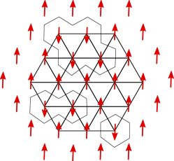
Figure 1: (Color online) A particular many-body configuration ${|\,{s^{(1)}}\,\rangle}$ of spins $Z^{(1)}_{j}$ (red), where the loops are defined along the domain walls and have support on the dual lattice. As in Ref. Levin-2012, , in order to determine the projection of the $\mathbb{Z}_{2}$ symmetry on the edge, we take the outer spins in a reference state where they are all pointing up.

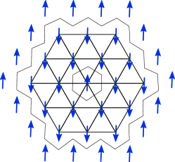
Figure 2: (Color online) A particular many-body configuration ${|\,{s^{(2)}}\,\rangle}$ of spins $Z^{(2)}_{j}$ (blue).

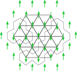
Figure 3: (Color online) A particular many-body configuration ${|\,{s^{(12)}}\,\rangle}$ of the spins $Z^{(12)}_{j}=Z^{(1)}_{j}\,Z^{(2)}_{j}$ (green). Note how the direction of the arrows at every site is consistent with Figs. 1 and 2.

In Ref. J-Wang-2014, , the classification of two dimensional bosonic SPT states with $\mathbb{Z}_{n}\times\mathbb{Z}_{m}$ symmetry was studied from the point of view of the effective one dimensional edge degrees of freedom. The non-trivial SPT edge states were there shown to be associated with non-trivial $3$-cocycles in the group cohomology. However, no microscopic theory for the two-dimensional bulk states has been investigated. In this section, we construct a microscopic theory for the $\mathbb{Z}_{2}\times\mathbb{Z}_{2}$ bosonic SPT states using the formalism of RK Hamiltonians and show how the topological properties of the ground state give rise to the edge physics studied in Ref. J-Wang-2014, .

In addressing SPT states with $\mathbb{Z}_{2}\times\mathbb{Z}_{2}$ symmetry, we allow, at each site $j$ of the lattice, two spin species represented by Pauli operators $\{\,X^{(1)}_{j},Y^{(1)}_{j},Z^{(1)}_{j}\,\}$ and $\{\,X^{(2)}_{j},Y^{(2)}_{j},Z^{(2)}_{j}\,\}$, where the $\mathbb{Z}_{2}\times\mathbb{Z}_{2}$ symmetry is generated by

$$\begin{split}\widehat{S}^{(1)}_{\mathbb{Z}_{2}}=\prod_{j}\,X^{(1)}_{j}\,,\quad\widehat{S}^{(2)}_{\mathbb{Z}_{2}}=\prod_{j}\,X^{(2)}_{j}\,.\end{split}\textbullet$$ (61)

•

We immediately realize that there should exist at least four kinds of paramagnets, which are obtained by stacking two decoupled $\mathbb{Z}_{2}$ symmetric systems. These four states of matter are parametrized by two integer numbers, $p_{1},p_{2}\in\{0,1\}$, which contribute to the expansion of the ground state with the (real) phase factor $\exp{\left\{i\,\pi\,\left[p_{1}\,L(s^{(1)})+p_{2}\,L(s^{(2)})\right]\right\}}$, where $L(s^{(1)})$ and $L(s^{(2)})$ count, respectively, the number of loops defined by domain wall configurations formed by spins of species $1$ and $2$, as in Figs. 1 and 2.

In order to obtain $\mathbb{Z}_{2}\times\mathbb{Z}_{2}$ symmetric states that go beyond the tensor product of two $\mathbb{Z}_{2}$ symmetric states, we realize that, at each site $j$, we can consider an independent Ising spin $Z^{(12)}_{j}\equiv Z^{(1)}_{j}\,Z^{(2)}_{j}$ with eigenvalues $s^{(12)}_{j}=s^{(1)}_{j}\,s^{(2)}_{j}$.

We then propose

$$\begin{split}{|\,{\Psi^{2\mathrm{d}}_{\mathbb{Z}_{2}\times\mathbb{Z}_{2}}}\,\rangle}=\frac{1}{2^{N_{\mathrm{s}}}}\,\sum_{s^{(1)}}\,\sum_{s^{(2)}}\,e^{i\,\pi\,\left[p_{1}\,L(s^{(1)})+p_{2}\,L(s^{(2)})+p_{12}\,L(s^{(12)})\right]}\,{|\,{s^{(1)};s^{(2)}}\,\rangle}\,\end{split}\textbullet$$ (62)

• as a description of the $8$ classes of $\mathbb{Z}_{2}\times\mathbb{Z}_{2}$ symmetric ground states parametrized by $3$ binary indices $p_{1},p_{2},p_{12}\in\{0,1\}$. We adopt the notation ${|\,{s^{(1)}}\,\rangle}\otimes{|\,{s^{(2)}}\,\rangle}\equiv{|\,{s^{(1)};s^{(2)}}\,\rangle}$. When $p_{1}=p_{2}=p_{12}=0$, Eq. (62) describes the trivial ground state

$$\begin{split}{|\,{\Phi^{2\mathrm{d}}_{\mathbb{Z}_{2}\times\mathbb{Z}_{2}}}\,\rangle}=\frac{1}{2^{N_{\mathrm{s}}}}\,\sum_{s^{(1)}}\,\sum_{s^{(2)}}\,{|\,{s^{(1)};s^{(2)}}\,\rangle}\,,\end{split}\textbullet$$ (63)

• which is the tensor product of two trivial $\mathbb{Z}_{2}$ paramagnets.

Eq. (62) corresponds to the choice of ground state in the “high temperature” limit $\beta=0$ and the SPT ground states can be obtained from the trivial one, Eq. (63), via the unitary transformation $\mathbb{W}^{2\mathrm{d}}_{\mathbb{Z}_{2}\times\mathbb{Z}_{2}}$, whose action on the many-body basis $\{\,{|\,{s^{(1)};s^{(2)}}\,\rangle}\,\}$ reads

$$\mathbb{W}^{2\mathrm{d}}_{\mathbb{Z}_{2}\times\mathbb{Z}_{2}}\,{|\,{s^{(1)};s^{(2)}}\,\rangle}\equiv e^{i\,W^{2\mathrm{d}}_{\mathbb{Z}_{2}\times\mathbb{Z}_{2}}(s^{(1)};s^{(2)})}\,{|\,{s^{(1)};s^{(2)}}\,\rangle}=e^{i\,\pi\,\left[p_{1}\,L(s^{(1)})+p_{2}\,L(s^{(2)})+p_{12}\,L(s^{(12)})\right]}\,{|\,{s^{(1)};s^{(2)}}\,\rangle}\,.$$ (64)

• In Eqs. (62) and (64), in order to simplify the notation, we omit the indices $p_{1}$, $p_{2}$ and $p_{12}$ on which the SPT ground states and the unitary transformation depend upon.

V.2.1 Parent Hamiltonians of the $\mathbb{Z}_{2}\times\mathbb{Z}_{2}$ state in $\mathrm{d}=2$

The Hamiltonian

$$\begin{split}H^{2\mathrm{d}}_{\mathbb{Z}_{2}\times\mathbb{Z}_{2}}=\omega_{0}\,\sum_{j}\,\left[\left(1-X^{(1)}_{j}\right)+\left(1-X^{(2)}_{j}\right)\right]\end{split}\textbullet$$ (65)

• describes a trivial paramagnetic system and has Eq. (63) as its ground state. It is the sum of two RK Hamiltonians of the form Eq. (11) with $\beta=0$, $\omega_{s,s^{\prime}}=\omega_{0}>0$, where the sum in Eq. (11a) extends over pairs of states $(s,s^{\prime})$ which differ by a single spin flip.

Then applying the unitary transformation $\mathbb{W}^{2\mathrm{d}}_{\mathbb{Z}_{2}\times\mathbb{Z}_{2}}$ in Eq. (64) to the Hamiltonian Eq. (65) yields the microscopic model realizing the $8$ classes of $\mathbb{Z}_{2}\times\mathbb{Z}_{2}$ SPT paramagnets:

$$\begin{split}\mathcal{H}^{2\mathrm{d}}_{\mathbb{Z}_{2}\times\mathbb{Z}_{2}}&\,=\mathbb{W}^{2\mathrm{d}}_{\mathbb{Z}_{2}\times\mathbb{Z}_{2}}\,H^{2\mathrm{d}}_{\mathbb{Z}_{2}\times\mathbb{Z}_{2}}\,\left(\mathbb{W}^{2\mathrm{d}}_{\mathbb{Z}_{2}\times\mathbb{Z}_{2}}\right)^{-1}\\ &\,=\omega_{0}\,\sum_{j}\,\Big{\{}1-X^{(1)}_{j}\,e^{i\,\pi\,\left(p_{1}+p_{12}\right)+i\,\frac{\pi}{4}\,\sum_{<\ell\,\ell^{\prime};\,j>}\,\left[p_{1}\,\left(1-Z^{(1)}_{\ell}\,Z^{(1)}_{\ell^{\prime}}\right)+p_{12}\,\left(1-Z^{(12)}_{\ell}\,Z^{(12)}_{\ell^{\prime}}\right)\right]}\Big{\}}\\ &\,+\omega_{0}\,\sum_{j}\,\Big{\{}1-\,X^{(2)}_{j}\,e^{i\,\pi\,\left(p_{2}+p_{12}\right)+i\,\frac{\pi}{4}\,\sum_{<\ell\,\ell^{\prime};\,j>}\,\left[p_{2}\,\left(1-Z^{(2)}_{\ell}\,Z^{(2)}_{\ell^{\prime}}\right)+p_{12}\,\left(1-Z^{(12)}_{\ell}\,Z^{(12)}_{\ell^{\prime}}\right)\right]}\Big{\}}\,,\end{split}\textbullet$$ (66)

• where the notation $<\ell\,\ell^{\prime};\,j>$ denotes that the summation in the exponent runs over pairs of nearest neighbors $\ell$ and $\ell^{\prime}$, which themselves belong to the $6$ nearest sites around a given site $j$ of the triangular lattice. When $p_{12}=0$ and $p_{1}=p_{2}=1$, Eq. (66) describes, up to an overall energy shift, two decoupled Levin-Gu Hamiltonians. Levin-2012 On the other hand, the case $p_{12}=1$ encodes strong entanglement between the two Ising systems.

V.2.2 Edge symmetry transformations of the $\mathbb{Z}_{2}\times\mathbb{Z}_{2}$ state in $\mathrm{d}=2$

The physical properties of the edge of two dimensional bosonic SPT states can be understood from the chiral action of the symmetry on the edge modes Lu-2012 ; Chen-2012-b ; Levin-2012 ; Santos-2014 ; J-Wang-2014 ; Else-2014 which, on a microscopic scale, originates from a non-onsite symmetry realization on the edge degrees of freedom. Chen-2012-b ; Levin-2012 ; Santos-2014 ; J-Wang-2014 For the $\mathbb{Z}_{2}\times\mathbb{Z}_{2}$ SPT states considered here, the non-onsite symmetry transformations on the edge were shown in Ref. J-Wang-2014, to be a manifestation of the non-trivial type-II cocycles of group cohomology.

The ground state Eq. (63) is a simple product state and, as such, the edge states are disentangled from the bulk. On the other hand, in the other SPT ground states whose expansion coefficients depend upon the domain wall configurations, the effect of flipping an edge spin can change the number of loops $L$, implying an entanglement between edge and bulk degrees of freedom. Therefore by studying the properties of the edge states, we can gain information about the nature of the bulk states and vice versa.

We have found, working directly with the bulk SPT wave functions Eq. (62), that the projection of the symmetry transformations Eq. (61) onto the boundary spins is

$$\begin{split}\widehat{S}^{(1)}_{\mathbb{Z}_{2},\textrm{edge}}=&\,\prod_{j}\,X^{(1)}_{j}\,e^{i\,\pi\,\left(p_{1}+p_{12}\right)+i\,\frac{\pi}{4}\,\left[p_{1}\left(1-Z^{(1)}_{j}\,Z^{(1)}_{j+1}\right)+p_{12}\left(1-Z^{(12)}_{j}\,Z^{(12)}_{j+1}\right)\right]}\,,\end{split}\textbullet$$ (67a)

•

$$\begin{split}\widehat{S}^{(2)}_{\mathbb{Z}_{2},\textrm{edge}}=&\,\prod_{j}\,X^{(2)}_{j}\,e^{i\,\pi\,\left(p_{2}+p_{12}\right)+i\,\frac{\pi}{4}\,\left[p_{2}\left(1-Z^{(2)}_{j}\,Z^{(2)}_{j+1}\right)+p_{12}\left(1-Z^{(12)}_{j}\,Z^{(12)}_{j+1}\right)\right]}\,,\end{split}\textbullet$$ (67b)

•

• where the product in Eq. (67) is taken over the spins on the edge with periodic boundary conditions. Remarkably these are the same non-onsite symmetry transformations studied in Ref. J-Wang-2014, , which shows that Eq. (62) gives the correct representation of the ground state of the two dimensional bosonic SPT states protected by $\mathbb{Z}_{2}\times\mathbb{Z}_{2}$ symmetry. As is clear from Eq. (67), the non-onsite form acquired by the edge symmetry in the non-trivial SPT phase implies that domain wall configurations on the edge carry projective representation of the $\mathbb{Z}_{2}$ symmetry, i.e., upon flipping any given spin configuration twice, there is a factor of $(-1)^{p}$ for every domain wall. Since the total number of domain walls is even, it follows that Eq. (67) is a faithful representation of the $\mathbb{Z}_{2}$ symmetry on the edge.

VI Conclusions and future directions

We have demonstrated that Rokhsar-Kivelson models offer a useful framework for constructing microscopic models whose ground states encode the universal properties of bosonic symmetry-protected topological states. Although we have illustrated our construction for one- and two-dimensional models and for certain discrete symmetries (unitary and anti-unitary), we believe our construction should hold true generically for any number of dimensions and for continuous symmetries as well. We close with a few observations:

1. It will certainly be interesting to realize parent Hamiltonians for bosonic SPT states in two dimensions with discrete symmetry $\mathbb{Z}_{n}$, for $n\geq 3$. In contrast to the $\mathbb{Z}_{2}$ case, the expansion of the paramagnetic state in the ordered basis contains more than one type of domain walls, suggesting that the coefficients in the expansion of the SPT ground state in the ${|\,{s}\,\rangle}$ basis may depend on orientable loops. It remains an open question how these domain wall fluctuations can coherently give rise to SPT ground states.

2. We expect that this formalism may offer a path to constructing microscopic models for other classes of bosonic SPT states in three dimensions, as well as interesting examples of bosonic SPT states in two dimensions protected by $\mathbb{Z}_{2}\times\mathbb{Z}_{2}\times\mathbb{Z}_{2}$ symmetry, which are classified by non-trivial Type-III cocycles. J-Wang-2014

3. A refinement of the group cohomology classification in terms of cobordisms has been recently proposed to describe three dimensional bosonic SPT states with time-reversal symmetry. Kapustin-2014 It could be worthwhile to study these time-reversal symmetric phases of matter using the formalism of RK Hamiltonians, in particular, to understand if there is any special meaning attached to the global unitary transformation that connects the trivial and the non-trivial SPT ground states, which could shed new light on the reason behind the inability of the group cohomology classification to account for these phases of matter.

Appendix A $\mathbb{Z}_{n}$ operators

At each site $j$ of a lattice we consider operators $\sigma_{j}$ and $\tau_{j}$ represented by $n\times n$ matrices

$$\sigma_{j}=\begin{pmatrix}1&0&0&0\\ 0&\omega&0&0\\ 0&0&\ddots&0\\ 0&0&0&\omega^{n-1}\end{pmatrix}\,,$$ (68)

•

$$\tau_{j}=\begin{pmatrix}0&0&0&\dots&0&1\\ 1&0&0&\dots&0&0\\ 0&1&0&\dots&0&0\\ 0&0&1&\dots&0&0\\ \vdots&0&0&\dots&1&0\end{pmatrix}\,,$$ (69)

• satisfying

$$\begin{split}{\sigma}^{n}_{j}=\tau^{n}_{j}=1\,,\quad\tau^{\dagger}_{j}\,{\sigma}_{j}\,\tau_{j}=\omega\,{\sigma}_{j}\,,\end{split}\textbullet$$ (70)

• where $\omega=e^{i\,\frac{2\,\pi}{n}}$ and $\bar{\omega}=e^{-i\,\frac{2\,\pi}{n}}$.

The following identities hold for $p=0,...,n$:

$$\begin{split}\exp{\left\{i\,\frac{2\,\pi p}{n}\,\left[\frac{n-1}{2}+\sum^{n-1}_{a=1}\,\frac{\left({\sigma}^{\dagger}_{j}\,{\sigma}_{j^{\prime}}\right)^{a}}{\bar{\omega}^{a}-1}\right]\right\}}=\left({\sigma}^{\dagger}_{j}\,{\sigma}_{j^{\prime}}\right)^{p}\,,\end{split}\textbullet$$ (71)

•

$$\begin{split}\exp{\left\{-i\,\frac{2\,\pi p}{n}\,\left[\frac{n-1}{2}+\sum^{n-1}_{a=1}\,\frac{\left({\sigma}^{\dagger}_{j}\,{\sigma}_{j^{\prime}}\right)^{a}}{\omega^{a}-1}\right]\right\}}=\left({\sigma}^{\dagger}_{j}\,{\sigma}_{j^{\prime}}\right)^{p}\,.\end{split}\textbullet$$ (72)

•

References

- (1) F. D. M. Haldane, Phys. Lett. 93A, 464 (1983).
- (2) F. D. M. Haldane, Phys. Rev. Lett. 50, 1153 (1983).
- (3) F. D. M. Haldane, J. Appl. Phys. 57, 3359 (1985).
- (4) I. Affleck, T. Kennedy, E. H. Lieb, and H. Tasaki, Phys. Rev. Lett. 59, 799 (1987).
- (5) I. Affleck, T. Kennedy, E. H. Lieb, and H. Tasaki, Comm. Math. Phys. 115, 477 (1988).
- (6) X. Chen, Z.-C. Gu, Z.-X. Liu, and X.-G. Wen, Science 338, 1604 (2012).
- (7) X. Chen, Z. -C. Gu, Z. -X. Liu and X. -G. Wen, Phys. Rev. B 87, 155114 (2013).
- (8) Y.-M. Lu and A. Vishwanath, Phys. Rev. B 86, 125119 (2012).
- (9) X. Chen and X. -G. Wen, Phys. Rev. B 86, 235135 (2012).
- (10) A. Vishwanath and T. Senthil, Phys. Rev. X 3, 011016 (2013).
- (11) M. A. Metlitski, C. L. Kane, and Matthew P. A. Fisher, Phys. Rev. B 88, 035131 (2013).
- (12) O. M. Sule, X. Chen, and S. Ryu, Phys. Rev. B 88, 075125 (2013).
- (13) C. Wang, A. Potter, and T. Senthil, Science 343, 629 (2014).
- (14) P. Ye and J. Wang, Phys. Rev. B 88, 235109 (2013).
- (15) L. H. Santos and J. Wang, Phys. Rev. B 89, 195122 (2014).
- (16) J. Wang, L. H. Santos, and X.-G. Wen, arXiv:1403.5256 (unpublished).
- (17) C. Xu and T. Senthil, Phys. Rev. B 87, 174412 (2013).
- (18) Zhen Bi, Alex Rasmussen, Cenke Xu, Phys. Rev. B 91, 134404 (2015).
- (19) X. Chen, Z.-X. Liu, and X.-G. Wen, Phys. Rev. B 84, 235141 (2011).
- (20) M. Levin and Z.-C. Gu, Phys. Rev. B 86, 115109 (2012).
- (21) X. Chen, Y.-M. Lu, and A. Vishwanath, Nat. Comm. 5, 3507 (2014).
- (22) F. J. Burnell, X. Chen, L. Fidkowski, and A. Vishwanath, arXiv:1302.7072 (unpublished).
- (23) L. Fidkowski, X. Chen and A. Vishwanath, Phys. Rev. X 3, 041016 (2013).
- (24) Y.-M. Lu and D.-H. Lee, Phys. Rev. B 89, 205117 (2014).
- (25) X. Chen, F. J. Burnell, A. Vishwanath and L. Fidkowski, arXiv:1403.6491 (unpublished).
- (26) S. D. Geraedts and O. I. Motrunich, arXiv:1410.1580
- (27) D. S. Rokhsar and S. A. Kivelson, Phys. Rev. Lett. 61, 2376 (1988).
- (28) C. L. Henley, J. Stat. Phys. 89, 483 (1997).
- (29) E. Ardonne, P. Fendley, and E. Fradkin, Annals of Physics (N.Y.) 310, 493 (2004).
- (30) C. L. Henley, J. Phys.: Condens. Matter 16, S891 (2004).
- (31) C. Castelnovo, C. Chamon, C. Mudry, and P. Pujol, Annals of Physics 318, 316 (2005).
- (32) M. E. Fisher and J. Stepheson, Phys. Rev. 132, 1411 (1963).
- (33) D. V. Else and C. Nayak, Phys. Rev. B 90, 235137 (2014).
- (34) A. Kapustin, arXiv:1403.1467; arXiv:1404.6659 (unpublished).