Connecting Faint End Slopes of the Lyman- emitter and Lyman-break Galaxy Luminosity Functions
Abstract
We predict Lyman- (Ly) luminosity functions (LFs) of Ly-selected galaxies (Ly emitters, or LAEs) at using the phenomenological model of Dijkstra & Wyithe (2012). This model combines observed UV-LFs of Lyman-break galaxies (LBGs, or drop out galaxies), with constraints on their distribution of Ly line strengths as a function of UV-luminosity and redshift. Our analysis shows that while Ly LFs of LAEs are generally not Schechter functions, these provide a good description over the luminosity range of . Motivated by this result, we predict Schechter function parameters at . Our analysis further shows that (i) the faint end slope of the Ly LF is steeper than that of the UV-LF of Lyman-break galaxies, (with a median at ), and (ii) a turn-over in the Ly LF of LAEs at Ly luminosities erg s erg s-1 may signal a flattening of UV-LF of Lyman-break galaxies at . We discuss the implications of these results – which can be tested directly with upcoming surveys – for the Epoch of Reionization.
keywords:
galaxies: high-redshift – galaxies: luminosity function, mass function – cosmology: reionization – ultraviolet: galaxies1 Introduction
The luminosity function (LF) of galaxies provides one of the most basic statistical descriptions of a population of galaxies. It describes the number density of galaxies in a given luminosity interval. Generally, the LF is well described by a Schechter (1976) function
| (1) |
with a normalization parameter , an exponential cutoff at , and, a power law with faint-end-slope for . The parameters depend on wavelength considered, galaxy type (e.g., passive versus star forming), and cosmic time.
At high redshift, galaxies are typically identified either through their broadband colors, for example using the drop-out or Lyman-break technique (Steidel et al., 1996), or through narrow-band searches aimed at detecting emission lines (Partridge & Peebles, 1967; Djorgovski et al., 1985) In particular, young star forming galaxies emit a significant fraction of their radiation as Lyman- (Ly) emission, and this method has been proved to be very efficient in finding samples out to (e.g. Rhoads et al., 2000; Rhoads & Malhotra, 2001; Ouchi et al., 2008; Bond et al., 2009; Bond et al., 2010; Guaita et al., 2010; Kashikawa et al., 2011; Hibon et al., 2012; Ono et al., 2012; Ota & Iye, 2012; Rhoads et al., 2012; Shibuya et al., 2012; Finkelstein et al., 2013; Konno et al., 2014).
Galaxies that have been selected (found) on the basis of their Ly lines are referred to as ‘Ly emitters’ (or LAEs). LAEs are useful because they are selected on having a strong Ly line flux irrespective of their associated UV-continuum emission. Therefore, LAEs can be fainter in the continuum compared to Lyman-break galaxies, and complement galaxy samples obtained via broadband searches which have been extensively carried out with the Hubble Space Telescope out to (e.g. Yan & Windhorst, 2004; Beckwith et al., 2006; Bouwens et al., 2006; Wilkins et al., 2010; Trenti et al., 2011; Grazian et al., 2012; Finkelstein et al., 2012; Bouwens et al., 2014a; Finkelstein et al., 2014; Oesch et al., 2014; Schmidt et al., 2014). Moreover, the sensitivity of the observed Ly flux to intervening neutral hydrogen gas makes LAEs an excellent probe of the Epoch of Reionization (see e.g. Dijkstra, 2014, for a review).
Since the range of observed Ly luminosities at high- typically extends only over orders of magnitude, the shape of the Ly LF is not strongly constrained and a fit with a Schechter function leads to significant degeneracy in the parameters. In particular the faint-end slope is essentially unconstrained: for example, Henry et al. (2012) used a sample of six (three) LAEs to find () at . Other approaches include assuming a fixed value for and resorting to the data to constrain the other parameters (van Breukelen et al., 2005; Dawson et al., 2007; Ouchi et al., 2008; Hu et al., 2010; Kashikawa et al., 2011; Ciardullo et al., 2012; Zheng et al., 2013). In contrast, the ultraviolet (UV) LF of Lyman-break galaxies (LBGs) is much better constrained due to available data stretching over several orders of magnitude in luminosity (McLure et al., 2010; Yan et al., 2011; Bouwens et al., 2011; Bradley et al., 2012; Oesch et al., 2012; Yan et al., 2012; Lorenzoni et al., 2013; Schenker et al., 2013). For the faint end slope, the most recent by Bouwens et al. (2014a) finds () at ().
There exists a clear opportunity to connect LAEs and LBGs via the Ly line emission properties of LBGs. Shapley et al. (2003) provided a probability distribution function (PDF) of the rest-frame equivalent-width (EW) of the Ly line in their sample of LBGs. Dijkstra & Wyithe (2012) showed that this observed PDF was well described by an exponential function, and that the characteristic scale-length of this function increased towards fainter UV-luminosities. While there do not exist equally well measured PDFs at higher redshifts and/or fainter UV-luminosities, recent studies have constrained both the redshift and UV-luminosity dependence of the so-called ‘Ly fraction’, which quantifies the fraction of LBGs for which the Ly EW exceeds a certain value. The Ly fractions – which represent integrated versions of the full EW PDF – increase from to at fixed (Stark et al., 2010; Cassata et al., 2015) and from UV-bright to UV-faint galaxies (Stark et al., 2010; Stark et al., 2011; Pentericci et al., 2011; Ono et al., 2012; Schenker et al., 2012).
There have been several attempts to link the redshift evolution of LBGs and their Ly fractions to LAE luminosity functions (Dijkstra & Wyithe, 2012; Faisst et al., 2014; Schenker et al., 2014). In this paper, we follow the work of Dijkstra & Wyithe (2012) and combine the most recent constraints on UV-LFs & Ly fractions to make predictions for Ly LFs. Dijkstra & Wyithe (2012) showed that this phenomenological model reproduces observed Ly LFs and their redshift evolution remarkably well. Here, we focus specifically on the faint-end slope of the Ly LF of LAEs, because (i) we can make robust predictions for this faint end slope, (ii) as we will show later, this faint end slope can be highly relevant for understanding the Epoch of Reionization.
2 Method
The number density of LAEs with luminosities in the interval is given by
| (2) |
Here, denotes the number density of LBGs as a function of in the range . This function can be represented by the Schechter function with parameters .
The term is the conditional probability that a galaxy has a Ly luminosity given an absolute UV magnitude . This conditional probability can be recast in terms of the equivalent width () probability density function as if , where and are related as . Here, the luminosity/flux densities, frequency and wavelength are evaluated just longward of the Ly resonance at Å. We can extrapolate these flux/luminosities to their values where the UV-continuum measurements are usually made (see e.g. Dijkstra & Westra 2010)111We use the relation where is the UV luminosity density and converts the flux density at Å to that at Å, which is the wavelength where was measured (Dijkstra & Westra, 2010).. Furthermore, denotes the equivalent width threshold that determines whether a galaxy would make it into an LAE sample. We adopt that Å, but note that some surveys adopt colour criteria for selecting LAEs as large as Å (see Dijkstra & Wyithe, 2012). If , then since in this case the galaxy does not qualify as an LAE. This threshold more closely represents detection threshold for Ly emitting galaxies in spectroscopic surveys222Note that in practise an EW cut is likely still needed to distinguish between LAEs and lower- interlopers, such as [OII] emitters. This EW cut can nevertheless be lower than Å (Leung et al., 2015) – e.g., with MUSE (Bacon et al., 2010), HETDEX (Hill et al., 2008) and/or VIMOS (Cassata et al., 2011, 2015). We have verified that our main results do not depend on this choice333We have verified that varying in the range Å changes by ..
The preceding factor in Eq. (2) is merely a normalization constant to fit the data and, hence, can be thought of as the ratio of predicted versus the total number of LAEs. This factor should ideally be . However, Dijkstra & Wyithe (2012) required that . The origin of this number is not known (see Dijkstra & Wyithe, 2012, for an extensive discussion)444The value of depends weakly on the adopted UV Schechter function parameters. For example, Bowler et al. (2014) reported slightly different best-fit values, which drive up to . The Finkelstein et al. (2014) parameters, on the other hand, also suggest ., but we stress it only affects the predicted normalization linearly and not the predicted faint-end slopes.
Hence, the key function in our analysis is . Several functional forms have been explored in the literature. Schenker et al. (2014) compared the maximum likelihood values for several EW distributions to their Keck MOSFIRE (McLean et al., 2012) data, and concluded that the exponential distribution introduced by Dijkstra & Wyithe (2012) provides an adequate fit. This functional form is
| (3) |
with where , , , , and are model parameters. These parameters were chosen to match the observations of (Shapley et al., 2003) and Stark et al. (2010); Stark et al. (2011) as closely as possible. Furthermore, is a normalization constant which is forced to be zero outside of . Our choice of values for the model parameters is described in Sec. 3.3 where we present the numerical results. In Appendix A we show explicitly that the main results in this paper are insensitive to both the functional form of and the parameterization of .
3 Results
We first present results in which EWconstant (in § 3.1). This allows us to demonstrate that for models in which the Ly fraction does not evolve with , the faint end slope of the LF of LAEs approaches that of LBGs. We then present a simplified model in § 3.2 in which the mean Ly EW-PDF increases towards fainter UV-luminosity function. This model demonstrates quantitatively that the faint end slope of the LF of LAEs is steeper than that of LBGs if the Ly fraction increases towards fainter UV-luminosities. In § 3.3 we present the results that we obtained from the EW-PDF given in Eq. (3).
3.1 Exemplary case with
We consider the case , i.e. . Furthermore, we set for . Under these assumptions we find
| (4) | ||||
| (5) |
where is the modified Bessel function of the second kind and is the luminosity corresponding to .
Eq. (5) shows that the Ly LF generally does not take-on a Schechter form. The slope of the LF is given by
| (6) |
with . For we have , and we obtain to leading order . Thus, having a constant corresponds to an unchanged faint end slope, .

3.2 Exemplary case where evolves with
If depends on a general analytic solution for does not exist. For illustration purposes we first consider a case in which we replace Eq. (3) with a Dirac- distribution,
| (7) |
where . The parameter EWd can be interpreted as the mean of the full PDF. This -function PDF leads555For simplicity, we set the minimum and maximum UV luminosity to zero and infinity, respectively. to
| (8) |
Here, the faint end slope is . he Ly LF thus has a steeper faint-end slope than the LBG LF, if (i.e. if decreases towards fainter , as has been observed). Also note that we again obtain if does not evolve with .
3.3 Realistic case with inferred from observations
For the model parameters of in Eq. (3) we adopt the values from Dijkstra & Wyithe (2012)666Specifically the model parameters related to are given by . The EW-PDF covers the range []. Here, the lower limit , where follows the form Å for , Å for and Å, otherwise (see Dijkstra & Wyithe 2012). We used Å but we verified that this choice does not affect our results quantitatively.. Example EW-PDFs are shown in Appendix A.1. For a more detailed motivation of this we refer the reader to Dijkstra & Wyithe (2012). We integrate the UV-LF over the range when predicting Ly luminosity functions, and discuss the impact of varying in Sec. 4.
The redshift evolution of the best fit Schechter parameters of the UV LF is taken from Bouwens et al. (2014a) and given as , , and, . Following these analyses, we use Å as rest frame wavelength in which the UV continuum was measured and assume a UV spectral slope . This choice for does not affect our results (see Appendix A.4 for detailed discussion).
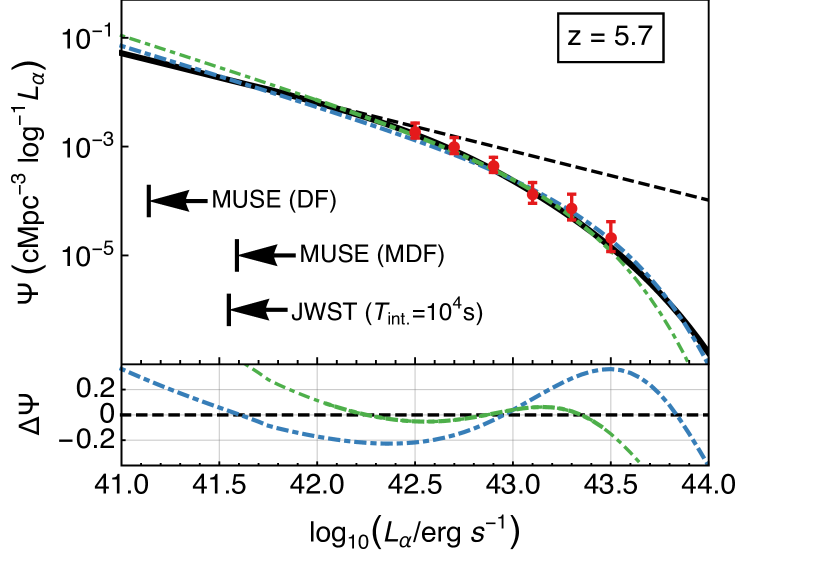
The upper panel of Fig. 1 shows the resulting number density of LAEs at in the luminosity range , i.e., , as a function of . This quantity is related to as (‘’ denotes the natural logarithm). We compare these prediction to the data from Ouchi et al. (2008). In addition, we show the MUSE detection limits777MUSE survey limits taken from http://muse.univ-lyon1.fr/IMG/pdf/science_case_gal_formation.pdf. for its medium deep field (MDF, limiting flux , integration time h), and, deep field (DF, , h) surveys as well as an exemplary JWST888JWST survey limits obtained from http://www.stsci.edu/jwst/science/sensitivity/ limit (, s).
Figure. 1 also shows two Schechter function approximations to our numerical findings fitted over the full luminosity-range shown (in blue) and over (in green). Although we do not expect the resulting Ly LF to be a Schechter function (as shown in Sec. 3.2), it provides a reasonable fit over the displayed luminosity range. This can also be seen in the lower panel of Fig. 1, where we display the relative deviation of the fits to the LF.
Fig. 2 shows the redshift evolution of the Schechter best fit parameters (as black lines). Predictions for do not account for reionization effects and are calculated with an unaltered EW evolution (solid line) as well as an EW-PDF which does not evolve after (dash-dotted line). We discuss this result separately in § 4.3. For comparison, we plot the corresponding redshift parameterization of the UV LF by Bouwens et al. (2014a) (as blue dashed lines). The left panel shows that increases by a factor over the redshift range , which differs from the redshift evolution in the characteristic UV-luminosity which drops by . This difference is driven by the redshift evolution in the Ly EW-PDF, which in turn was inferred from the observed redshift-evolution of Ly ‘fractions’ over this redshift range. The central panel shows that . This is again a consequence of inferred redshift evolution of the Ly-EW PDF (see § 3.2). This figure also illustrates the close-to-linear – relation. This evolution is mostly driven by the redshift evolution of . Finally, the right panel shows the predicted redshift evolution in .

4 Discussion
4.1 Low- turnover
The integral over diverges for . We therefore expect that the luminosity function flattens or turns-over below some luminosity. The minimum luminosity that we can account for in our models is
| (9) |
where Å (see footnote 6 in § 3.3) denotes the minimum equivalent width in our EW-PDF at the maximum absolute UV-magnitude (i.e. the lowest UV-luminosity). For example, we obtain for . At this luminosity we expect the predicted Ly luminosity to go to zero, as is shown in Figure 4.
An estimate for where we may start to see departures from a power-law slope can be obtained by considering the conditional probability . Bayes’ theorem states that , of which we show examples in Fig. 3 for four different values of . This Figure illustrates for example that Ly observations that probe a flux corresponding to erg s-1 – a level that can be reached in MUSE ultra deep fields – effectively probe galaxies with , which are fainter than can be probed directly even with the JWST. The JWST detection limit shown in Figure 3 is taken from Windhorst et al. (2006). Figure 3 further shows that if the UV-LF flattens off at – say – that then the effects should become noticeable in the predicted Ly luminosity function around erg s-1, as here galaxies with dominate the contribution to the Ly LF.
In Figure 4 we make these points more explicit, and show the predicted faint end of the LAE LF for four values of (calculated with the UV LF parameters at ). For each curve we marked with dotted lines. For example, a potential UV turnover at leads to deviations999The first deviations in the Ly LF can be found at with . Here, describes the half width of at a chosen probability threshold. of the Ly LF at and a cutoff at . Figure 4 also contains data points taken from Rauch et al. (2008). Rauch et al. (2008) performed an ultra deep (-hr) exposure with VLTs FORS2 low resolution spectrograph. The goal of these observations was to detect fluorescent Ly emission from optically thick clouds powered by the ionizing background. While their sensitivity turned out not to be good enough to detect this fluorescent emission (revised estimates of the ionizing background and the conversion efficiency into Ly), they detected numerous ultra faint Ly emitting sources characterizing their LF down to . We computed the uncertainties with the cosmic variance calculator of Trenti & Stiavelli (2008). These data-points fall on the predicted LF for . However we caution that the turn-over occurs at the lowest luminosity data-point only, which might suffer from incompleteness (although it lies above the detection threshold). In the same figure we provide the estimated MUSE limits for the deep field (DF) and the gravitationally lensed ultra deep field (UDF) surveys.

4.2 Implications for the Epoch of Reionization
Low luminosity galaxies are expected to play a major role in driving the reionization of the Universe (e.g. Robertson et al., 2010; Trenti et al., 2010; Kuhlen & Faucher-Giguère, 2012; Boylan-Kolchin et al., 2014). Determining the faint end of the LF such as its slope and a turnover luminosity is essential for constraining the volume emissivity of ionizing photons. However, even future experiments will have difficulties detecting these galaxies directly via their UV continuum flux. Current constraints rely, therefore, on extrapolation of local properties to higher redshifts (Weisz et al., 2014), (relatively few) gravitationally lensed objects (Alavi et al., 2014; Atek et al., 2014) or inferences from gamma-ray burst observations (Trenti et al., 2012). In this work, we have shown that the Ly LF can provide an independent probe of the faint end of the UV LF, and that for example the MUSE DF survey could already detect (or rule out) a turnover at .
Recent studies have shown that Ly escape may be correlated with the escape of ionizing photons (Behrens et al., 2014; Verhamme et al., 2014), as the escape of ionizing photons requires low HI-column density ( cm-2) channels, which can also provide escape routes for Ly photons. The fact that Ly LFs are likely steeper than the UV LFs implies that the Ly volume emissivity – and therefore possibly the ionizing emissivity – are weighted more strongly towards low luminosity galaxies. This is consistent with the expectation that ionizing photons escape more easily from lower mass – and hence lower luminosity – galaxies. A steep faint-end slope of the Ly LF may therefore provide observational support for this scenario.
4.3 Predictions for redshifts
We extrapolated our predictions for the best-fit Schechter parameters of the LAE LF to in two ways (shown in Fig. 2): (i) in the first, we assume that the EW-PDF continues to evolve as inferred from the observations at . This model is represented by the solid lines, and, (ii) in the second, we ‘freeze’ the EW distribution for at the value it had at (dashed lines). This latter assumption has been common in previous works (see e.g. Dijkstra et al., 2011; Bolton & Haehnelt, 2013; Jensen et al., 2013; Choudhury et al., 2014; Mesinger et al., 2015). We show results for these two models to get a sense for the uncertainties on our predictions. We stress that we have purposefully not modelled the impact of reionization on the EW-PDF. Reionization is likely responsible for the observed ‘drop’ in the observed Ly fractions at (e.g. Pentericci et al., 2011; Schenker et al., 2012; Ono et al., 2012; Treu et al., 2013; Caruana et al., 2014; Tilvi et al., 2014). Understanding this drop has been the main focus of previous works, and is outside the scope of this paper. Our predictions for are useful in a different way, as they provide predictions for the Ly LFs of LAEs in the absence of reionization. Comparison to observed LFs at these redshifts highlight the impact of reionization.
5 Conclusions
We predicted Ly luminosity functions (LFs) of Ly-selected galaxies (Ly emitters, or LAEs) at using the phenomenological model of Dijkstra & Wyithe (2012). This model combines observed UV-LFs of Lyman-break galaxies (LBGs), with observational constraints on the Ly EW PDF of these LBGs, as a function of and redshift. The results from our analysis can be summarized as follows:
-
•
While Ly luminosity functions of LAEs are generally not Schechter functions, these provide a good description over the luminosity range of (see Fig. 1).
-
•
We predict Schechter function parameters at (shown in Fig. 2). The faint end slope of the Ly LF is steeper than that of the UV-LF of LBGs, with a median at (see the central panel in Fig. 2). While the current work was in the advanced stage of completion, Dressler et al. (2014) posted a preprint in which they observationally infer a very steep faint end slope at (, also see Dressler et al. (2011)). The central value is in excellent agreement with the value predicted in our framework.
-
•
The faint end of the LAE LF provides independent constraints on the very faint end of the UV-LF of LBGs. For example, the predicted LAE LF at Ly luminosities erg s erg s-1 is sensitive to the UV-LF of LBGs in the range (see Fig. 3 and Fig. 4). These LBGs are too faint to be detected directly (even with JWST). A turn-over in the Ly LF of LAEs may signal a flattening of UV-LF of LBGs. We discuss implications of these results for the Epoch of Reionization in § 4.2.
We have verified that these results are insensitive to our assumed functional form of and how we parameterized its dependence on and . Our predictions can be tested directly with various upcoming surveys.
Acknowledgements
We thank Masami Ouchi for kindly providing the data points shown in Fig. 1. MD and MT thank Alan Dressler giving a presentation which inspired this work at the UCSB GLASS meeting in May 2014.
References
- Alavi et al. (2014) Alavi A., et al., 2014, ApJ, 780, 143
- Atek et al. (2014) Atek H., et al., 2014, ApJ, 786, 60
- Bacon et al. (2010) Bacon R., et al., 2010, in Society of Photo-Optical Instrumentation Engineers (SPIE) Conference Series. , doiXX:10.1117/12.856027
- Beckwith et al. (2006) Beckwith S. V. W., et al., 2006, AJ, 132, 1729
- Behrens et al. (2014) Behrens C., Dijkstra M., Niemeyer J., 2014, preprint (arXiv:1401.4860)
- Bolton & Haehnelt (2013) Bolton J. S., Haehnelt M. G., 2013, MNRAS, 429, 1695
- Bond et al. (2009) Bond N. A., Gawiser E., Gronwall C., Ciardullo R., Altmann M., Schawinski K., 2009, ApJ, 705, 639
- Bond et al. (2010) Bond N. A., Feldmeier J. J., Matković A., Gronwall C., Ciardullo R., Gawiser E., 2010, ApJ, 716, L200
- Bouwens et al. (2006) Bouwens R. J., Illingworth G. D., Blakeslee J. P., Franx M., 2006, ApJ, 653, 53
- Bouwens et al. (2011) Bouwens R. J., et al., 2011, ApJ, 737, 90
- Bouwens et al. (2014a) Bouwens R. J., et al., 2014a, preprint (arXiv:1403.4295)
- Bouwens et al. (2014b) Bouwens R. J., et al., 2014b, ApJ, 793, 115
- Bowler et al. (2014) Bowler R. A. A., et al., 2014, ArXiv e-prints,
- Boylan-Kolchin et al. (2014) Boylan-Kolchin M., Bullock J. S., Garrison-Kimmel S., 2014, MNRAS, 443, L44
- Bradley et al. (2012) Bradley L. D., et al., 2012, ApJ, 760, 108
- Caruana et al. (2014) Caruana J., Bunker A. J., Wilkins S. M., Stanway E. R., Lorenzoni S., Jarvis M. J., Ebert H., 2014, MNRAS, 443, 2831
- Cassata et al. (2011) Cassata P., et al., 2011, A&A, 525, A143
- Cassata et al. (2015) Cassata P., et al., 2015, A&A, 573, A24
- Choudhury et al. (2014) Choudhury T. R., Puchwein E., Haehnelt M. G., Bolton J. S., 2014, preprint (arXiv:1412.4790),
- Ciardullo et al. (2012) Ciardullo R., et al., 2012, ApJ, 744, 110
- Dawson et al. (2007) Dawson S., Rhoads J. E., Malhotra S., Stern D., Wang J., Dey A., Spinrad H., Jannuzi B. T., 2007, ApJ, 671, 1227
- Dijkstra (2014) Dijkstra M., 2014, PASA, 31, 40
- Dijkstra & Westra (2010) Dijkstra M., Westra E., 2010, MNRAS, 401, 2343
- Dijkstra & Wyithe (2012) Dijkstra M., Wyithe J. S. B., 2012, MNRAS, 419, 3181
- Dijkstra et al. (2011) Dijkstra M., Mesinger A., Wyithe J. S. B., 2011, MNRAS, 414, 2139
- Djorgovski et al. (1985) Djorgovski S., Spinrad H., McCarthy P., Strauss M. A., 1985, ApJ, 299, L1
- Dressler et al. (2011) Dressler A., Martin C. L., Henry A., Sawicki M., McCarthy P., 2011, ApJ, 740, 71
- Dressler et al. (2014) Dressler A., Henry A., Martin C. L., Sawicki M., McCarthy P., Villaneuva E., 2014, preprint (arXiv:1412.0655),
- Faisst et al. (2014) Faisst A. L., Capak P., Carollo C. M., Scarlata C., Scoville N., 2014, ApJ, 788, 87
- Finkelstein et al. (2012) Finkelstein S. L., et al., 2012, ApJ, 756, 164
- Finkelstein et al. (2013) Finkelstein S. L., et al., 2013, Nature, 502, 524
- Finkelstein et al. (2014) Finkelstein S. L., et al., 2014, preprint (arXiv:1410.5439),
- Grazian et al. (2012) Grazian A., et al., 2012, A&A, 547, A51
- Guaita et al. (2010) Guaita L., et al., 2010, ApJ, 714, 255
- Henry et al. (2012) Henry A. L., Martin C. L., Dressler A., Sawicki M., McCarthy P., 2012, ApJ, 744, 149
- Hibon et al. (2012) Hibon P., Kashikawa N., Willott C., Iye M., Shibuya T., 2012, ApJ, 744, 89
- Hill et al. (2008) Hill G. J., et al., 2008, in Kodama T., Yamada T., Aoki K., eds, Astronomical Society of the Pacific Conference Series Vol. 399, Panoramic Views of Galaxy Formation and Evolution. p. 115, arXiv:0806.0183
- Hu et al. (2010) Hu E. M., Cowie L. L., Barger A. J., Capak P., Kakazu Y., Trouille L., 2010, ApJ, 725, 394
- Jensen et al. (2013) Jensen H., Laursen P., Mellema G., Iliev I. T., Sommer-Larsen J., Shapiro P. R., 2013, MNRAS, 428, 1366
- Kashikawa et al. (2011) Kashikawa N., et al., 2011, ApJ, 734, 119
- Konno et al. (2014) Konno A., et al., 2014, preprint (arXiv:1404.6066),
- Kuhlen & Faucher-Giguère (2012) Kuhlen M., Faucher-Giguère C.-A., 2012, MNRAS, 423, 862
- Leung et al. (2015) Leung A. S., Gawiser E. J., Acquaviva V., Hetdex Collaboration 2015, in American Astronomical Society Meeting Abstracts. p. 336.49
- Lorenzoni et al. (2013) Lorenzoni S., Bunker A. J., Wilkins S. M., Caruana J., Stanway E. R., Jarvis M. J., 2013, MNRAS, 429, 150
- McLean et al. (2012) McLean I. S., et al., 2012, in Society of Photo-Optical Instrumentation Engineers (SPIE) Conference Series. , doiXX:10.1117/12.924794
- McLure et al. (2010) McLure R. J., Dunlop J. S., Cirasuolo M., Koekemoer A. M., Sabbi E., Stark D. P., Targett T. A., Ellis R. S., 2010, MNRAS, 403, 960
- Mesinger et al. (2015) Mesinger A., Aykutalp A., Vanzella E., Pentericci L., Ferrara A., Dijkstra M., 2015, MNRAS, 446, 566
- Oesch et al. (2012) Oesch P. A., et al., 2012, ApJ, 759, 135
- Oesch et al. (2014) Oesch P. A., et al., 2014, ApJ, 786, 108
- Ono et al. (2012) Ono Y., et al., 2012, ApJ, 744, 83
- Ota & Iye (2012) Ota K., Iye M., 2012, MNRAS, 423, 444
- Ouchi et al. (2008) Ouchi M., et al., 2008, ApJS, 176, 301
- Partridge & Peebles (1967) Partridge R. B., Peebles P. J. E., 1967, ApJ, 147, 868
- Pentericci et al. (2011) Pentericci L., et al., 2011, ApJ, 743, 132
- Rauch et al. (2008) Rauch M., et al., 2008, ApJ, 681, 856
- Rhoads & Malhotra (2001) Rhoads J. E., Malhotra S., 2001, ApJ, 563, L5
- Rhoads et al. (2000) Rhoads J. E., Malhotra S., Dey A., Stern D., Spinrad H., Jannuzi B. T., 2000, ApJ, 545, L85
- Rhoads et al. (2012) Rhoads J. E., Hibon P., Malhotra S., Cooper M., Weiner B., 2012, ApJ, 752, L28
- Robertson et al. (2010) Robertson B. E., Ellis R. S., Dunlop J. S., McLure R. J., Stark D. P., 2010, Nature, 468, 49
- Schechter (1976) Schechter P., 1976, ApJ, 203, 297
- Schenker et al. (2012) Schenker M. A., Stark D. P., Ellis R. S., Robertson B. E., Dunlop J. S., McLure R. J., Kneib J.-P., Richard J., 2012, ApJ, 744, 179
- Schenker et al. (2013) Schenker M. A., et al., 2013, ApJ, 768, 196
- Schenker et al. (2014) Schenker M. A., Ellis R. S., Konidaris N. P., Stark D. P., 2014, ApJ, 795, 20
- Schmidt et al. (2014) Schmidt K. B., et al., 2014, ApJ, 786, 57
- Shapley et al. (2003) Shapley A. E., Steidel C. C., Pettini M., Adelberger K. L., 2003, ApJ, 588, 65
- Shibuya et al. (2012) Shibuya T., Kashikawa N., Ota K., Iye M., Ouchi M., Furusawa H., Shimasaku K., Hattori T., 2012, ApJ, 752, 114
- Stark et al. (2010) Stark D. P., Ellis R. S., Chiu K., Ouchi M., Bunker A., 2010, MNRAS, 408, 1628
- Stark et al. (2011) Stark D. P., Ellis R. S., Ouchi M., 2011, ApJ, 728, L2
- Steidel et al. (1996) Steidel C. C., Giavalisco M., Pettini M., Dickinson M., Adelberger K. L., 1996, ApJ, 462, L17
- Tilvi et al. (2014) Tilvi V., et al., 2014, ApJ, 794, 5
- Trenti & Stiavelli (2008) Trenti M., Stiavelli M., 2008, ApJ, 676, 767
- Trenti et al. (2010) Trenti M., Stiavelli M., Bouwens R. J., Oesch P., Shull J. M., Illingworth G. D., Bradley L. D., Carollo C. M., 2010, ApJ, 714, L202
- Trenti et al. (2011) Trenti M., et al., 2011, ApJ, 727, L39
- Trenti et al. (2012) Trenti M., Perna R., Levesque E. M., Shull J. M., Stocke J. T., 2012, ApJ, 749, L38
- Treu et al. (2013) Treu T., Schmidt K. B., Trenti M., Bradley L. D., Stiavelli M., 2013, ApJ, 775, L29
- Verhamme et al. (2014) Verhamme A., Orlitova I., Schaerer D., Hayes M., 2014, preprint (arXiv:1404.2958)
- Weisz et al. (2014) Weisz D. R., Johnson B. D., Conroy C., 2014, preprint (arXiv:1409.4772)
- Wilkins et al. (2010) Wilkins S. M., Bunker A. J., Ellis R. S., Stark D., Stanway E. R., Chiu K., Lorenzoni S., Jarvis M. J., 2010, MNRAS, 403, 938
- Windhorst et al. (2006) Windhorst R. A., Cohen S. H., Jansen R. A., Conselice C., Yan H., 2006, New A Rev., 50, 113
- Yan & Windhorst (2004) Yan H., Windhorst R. A., 2004, ApJ, 612, L93
- Yan et al. (2011) Yan H., et al., 2011, ApJ, 728, L22
- Yan et al. (2012) Yan H., et al., 2012, ApJ, 761, 177
- Zheng et al. (2013) Zheng Z.-Y., et al., 2013, MNRAS, 431, 3589
- van Breukelen et al. (2005) van Breukelen C., Jarvis M. J., Venemans B. P., 2005, MNRAS, 359, 895
Appendix A Varying the EW distribution
In this appendix, we demonstrated that our main results and conclusions do not depend on our assumed EW-PDF.
A.1 Fiducial
Our default EW distribution is given by Eq. (3). We plot the PDF for three UV magnitudes and two redshifts in Fig. 5.

A.2 Schenker et al. (2014) parameterization
As mentioned in Sec. 2, Schenker et al. (2014) suggest an alternative parameterization of the EW-PDF, namely
| (10) |
This log-normal PDF possesses the parameters , and . The latter is given by
| (11) |
where is the UV continuum slope. Schenker et al. (2014) found their EW distribution to depend more strongly on than on , and therefore constrained . We can include this parameterization into our formalism if we map onto .
This mapping is based on three results from Bouwens et al. (2014b):
-
1.
We use their empirical linear correlation between at . This relation constrains .
-
2.
Furthermore, we apply their measured change per unit redshift .
-
3.
Finally, we use their measurement that () for ().
Accordingly, our mapping can be written as
| (12) |
where and .
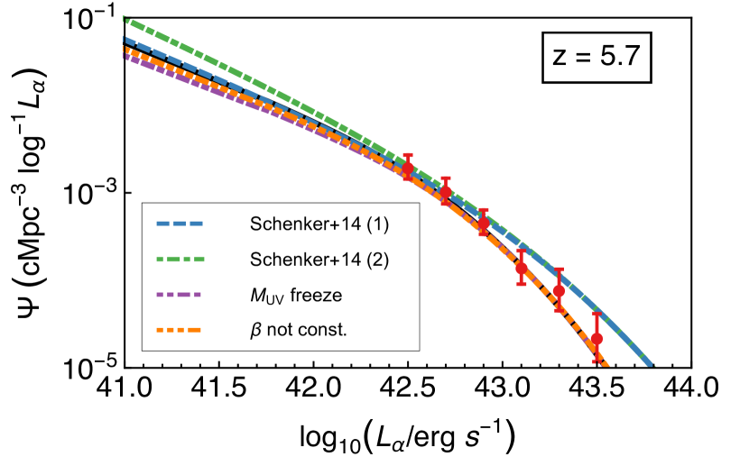
In Eq. (10) we used the best parameters by Schenker et al. (2014), i.e., . In addition, since is degenerate with , we set . The orange dashed line in Fig. 6 shows the resulting Ly LF at . The agreement in the faint-end between the two procedures is remarkable. For greater luminosities, however, the Schenker et al. (2014) parameterization leads to a (much) higher number density of LAEs. While there are significant uncertainties in the above procedure, the agreement we get at the faint end slope is especially encouraging. Future surveys can be extremely useful in further connecting the LAE and LBG populations by constraining the bright end of the LAE luminosity function.
A.3 ‘Freezing’ the EW PDF for faint galaxies
Since the evolution in the EW PDF for fainter sources involves a (modest) extrapolation of observationally inferred , we have also tested and alternative PDF where we ‘froze’ the evolution at . That is, we also conservatively assume that the EW-PDF stops evolving at (even though observations hint that this is not the case, see fig. 13 of Stark et al. (2010)). Fig. 6 shows the resulting Ly LF (purple line). It is clear that our results are only affected slightly, i.e., the faint-end-slope is reduced by . We also tested this over a variety of redshifts.
A.4 Non-constant UV spectral slope
The spectral slope is not a constant, but depends on UV magnitude and redshift (as discussed above). This introduces some additional dispersion in the predicted Ly flux at a fixed . However, varying within changes the Ly flux only by . This dispersion is smaller than that introduced by the EW-PDF. If we replace the constant with the empirical fit described in § A.2, then our predicted Ly LF (represented by the orange line in Fig. 6) is barely any different from our fiducial model that used (represented by the black solid line).