Gravitational Lens Modelling in a Citizen Science Context

Abstract

We develop a method to enable collaborative modelling of gravitational lenses and lens candidates, that could be used by non-professional lens enthusiasts. It uses an existing free-form modelling program (GLASS), but enables the input to this code to be provided in a novel way, via a user-generated diagram that is essentially a sketch of an arrival-time surface.

We report on an implementation of this method, SpaghettiLens, that has been tested in a modelling challenge using 29 simulated lenses drawn from a larger set created for the Space Warps citizen science strong lens search. We find that volunteers from this online community asserted the image parities and time ordering consistently in some lenses, but made errors in other lenses depending on the image morphology. While errors in image parity and time ordering lead to large errors in the mass distribution, the enclosed mass was found to be more robust: the model-derived Einstein radii found by the volunteers were consistent with those produced by one of the professional team, suggesting that given the appropriate tools, gravitational lens modelling is a data analysis activity that can be crowd-sourced to good effect. Ideas for improvement are discussed; these include (a) overcoming the tendency of the models to be shallower than the correct answer in test cases, leading to systematic over-estimation of the Einstein radius by 10% at present, and (b) detailed modelling of arcs.

1 Introduction

The first work on lens modelling (Young et al., 1981a, b) was developed after the discovery of the first two gravitational lenses (Walsh et al., 1979; Weymann et al., 1980), where a massive galaxy causes a background quasar to appear as two or four images. For the second lens to be discovered (PG1115+080), mass models scored an early success with the prediction that one of the lensed images seen would split further into two at higher resolution. That galaxies must sometimes cause multiple images had long been expected (Zwicky, 1937), and it had even been argued that the phenomenon could help measure cosmological parameters (Refsdal, 1964, 1966), but apparently nobody was expecting that lenses would need detailed modelling. The first observations, however, immediately stimulated models. The reason for that lies in the image separation. Recall that image separations are of order of the angular Einstein radius

$$\Theta_{\rm E}\sim\left(\frac{4GM}{c^{2}D_{L}}\right)^{1/2}\simeq 0.1^{\prime\prime}\left(\frac{M}{M_{\odot}}\right)^{1/2}\left(\frac{D_{L}}{\rm pc}\right)^{-1/2},$$ (1)

where $D_{L}$ is the distance to the lens, and $M$ its mass. A lensing galaxy with $M\sim 10^{11}\rm\,M_{\odot}$ at $\sim 1\rm\,Gpc$ would cause image separations of $\sim 1^{\prime\prime}$, which is comparable to the size of the galaxy; typically the lensed images are seen through the galaxy halo. Hence, the lensed images depend on the detailed mass distribution of the lensing galaxy. Galaxy lenses therefore require models of their mass distributions.

Since those early discoveries, more than 400 secure lenses are now known. Modelling of the mass distribution is part of any research using lenses, but so far no modelling study has spanned all known lenses. The largest single one (Koopmans et al., 2009) models 58 separate lenses to infer the distribution of dark matter around galaxies. In other work, Leier et al. (2011) combined lens models of 21 galaxies with models of their stellar populations, to find the relation between stars and dark matter, and Sereno & Paraficz (2014) modelled 18 time-delay lenses together to infer cosmological parameters.

Imaging surveys now under way aim to increase the inventory of lenses another ten or a hundred fold (see e.g. Marshall et al., 2005; Oguri & Marshall, 2010), with both automated and visual search techniques proposed (e.g. Marshall et al., 2009; More et al., 2012; Gavazzi et al., 2014). For example, Space Warps (Marshall et al, in prep; More et al, in prep) is a citizen science project in which volunteers are presented sky-survey images and are invited to identify lens candidates, by eye. Simulated lenses are mixed in with the data, both to help train volunteers on what to look for, and to provide measures of the effectiveness of the search. The motivation for Space Warps is to enable volunteers, some of whom had previously serendipitously identified lens candidates on earlier citizen-science surveys, either to make discoveries missed in automatic searches by software robots, or to perform the necessary inspection of an automatically-generated sample, for quality control. Robots can be built to be good at detecting lensing system in clean, uncrowded fields with high signal-to-noise, but in more general test situations, robots miss lenses (low completeness) or contaminate the results with non-lenses (low purity) (Marshall et al., 2009).

The encouraging early results from the first Space Warps lens search, carried out on the $\simeq 172$ square degree Canada-France-Hawaii Telescope Legacy Survey (CFHTLS) imaging by over 30,000 volunteers (Marshall et al, in prep; More et al, in prep) prompted the question: could the modelling of the lenses also be done by the volunteers? If so, modelling could help prioritise lens candidates at an early stage, which would be very useful with new wide-field and sensitive surveys, which will yield thousands of lens candidates. There are several software tools for lens modelling available, and work has been done on generic interfaces (e.g. Lefor, 2014). Some early designs for Space Warps included a prototype lens modelling tool (Naudus et al., 2010). Moreover, some Space Warps volunteers are quite experienced from earlier projects, having individually spent a thousand hours or more with data, and are very interested in more demanding projects. The interests of citizen-science communities are just beginning to be studied (e.g., Raddick et al., 2013), but it is clear that some volunteers welcome open-ended challenges, and sometimes these have led to new scientific results: one example is the discovery of an exceptional extra-solar planet (Schwamb et al., 2013); another is the development of new algorithms for protein folding (Khatib et al., 2011). All these are grounds for optimism. There is, however, a basic difficulty in strong gravitational lensing. Lensed images do not look much like their source, and still less do they resemble the lensing-mass distribution. To model a lens, one needs either to do a lot of random guessing, or to have a good intuition for what works.

In this paper, we propose a way around the difficulty, and report on a modelling test on Space Warps using simulated lenses. The three following sections are devoted to the concept, the implementation, and tests respectively.

In Section 2 we introduce a markup system for lensed images, which we call a “spaghetti diagram.” A spaghetti diagram resembles the visible image system, in a cartoon-like way, and at the same time it encodes the basis of a mass model. This supplies an intuitive link between the image system and the mass distribution, which look frustratingly different from each other. Spaghetti diagrams are essentially the saddle-point contours originally introduced to gravitational lensing by Blandford & Narayan (1986) as a way of classifying lensed images. They are sometimes shown as part of the output of lens models (for example Rusin et al., 2001; Keeton & Winn, 2003; Lubini & Coles, 2012). In the present work, however, spaghetti diagrams are the input through which the modeller tells the SpaghettiLens program what to do.

In Section 3 we describe the SpaghettiLens program, which implements the above scheme. SpaghettiLens is an interface to and extension of the GLASS framework for modelling lenses (Coles et al., 2014). We will not go into software details in this paper, instead concentrate on lens modelling per se, but we remark that SpaghettiLens is designed to be friendly to the forum style of citizen-science projects, and enables incremental collaborative model refinement by different people, without sacrificing any of the technical features of GLASS.

In Section 4 we describe a modelling challenge where a diverse sample of 29 simulated lenses was modelled multiple times by a small number of Space Warps volunteers using SpaghettiLens. The models were then examined in two ways. One was whether the spaghetti diagram was correct. The other was the recovery of the Einstein radius of the lens. In addition, we show some visual comparisons of the actual and recovered lens shape and radial profile, and identify some areas to improve. Profile and shape recovery with GLASS has been studied in more detail in (Coles et al., 2014).

Section 5 gives the general outlook and next steps.

2 Fermat’s principle and spaghetti diagrams

We first explain the lensing theory relevant to SpaghettiLens, following the formulation of gravitational lensing in terms of Fermat’s principle by Blandford & Narayan (1986).

2.1 Geometrical and gravitational time delays

Consider a lens at some redshift $z_{L}$ and let $(x,y)$ be planar coordinates at the lens, transverse to the line of sight. Let $\Sigma(x,y)$ be the mass distribution. It is a mass per unit area, i.e., density projected along the line of sight. The mass distribution is often given in a dimensionless form

$$\kappa(x,y)\propto\Sigma(x,y)$$ (2)

called the convergence. Let there be light, in the form of a more distant source, at redshift $z_{S}$, behind point $(x_{s},y_{s})$ on the lens.

We now imagine a virtual photon flying from the source to some $(x,y)$ on the lens, then changing direction and coming to the observer. Such a direction change would increase the light travel time compared to coming through $(x_{s},y_{s})$. The increased light travel time from the geometry of deflection would be

$$t_{\rm geom}(x,y)\propto(x-x_{s})^{2}+(y-y_{s})^{2},$$ (3)

assuming the delay is small compared to the total light travel time.

An additional delay of the photon comes from travelling through the curved spacetime at the lens. This gravitational time delay $t_{\rm grav}$ is related to the mass distribution of the lens. The relation is generally written as a two-dimensional Poisson equation, but an alternative expression, avoiding calculus, is as follows. The value of $t_{\rm grav}$ through $(x,y)$ equals its average value on the circumference of a small circle centred at $(x,y)$, plus a constant times the mass within that circle. The constant is $2G/c^{3}$ times the cosmological expansion factor $(1+z_{L})$. Thus

$$t_{\rm grav}(x,y)=\left\langle t_{\rm grav}(x_{\lower 0.99458pt\hbox{$\circ$}},y_{\lower 0.99458pt\hbox{$\circ$}})\right\rangle+(1+z_{L})\frac{2G}{c^{3}}M(x_{\lower 0.99458pt\hbox{$\bullet$}},y_{\lower 0.99458pt\hbox{$\bullet$}})\,.$$ (4)

We have used $(x_{\lower 0.99458pt\hbox{$\circ$}},y_{\lower 0.99458pt\hbox{$\circ$}})$ to denote the circumference of a circle, and $(x_{\lower 0.99458pt\hbox{$\bullet$}},y_{\lower 0.99458pt\hbox{$\bullet$}})$ to indicate the integrated mass within the circle. Appendix A relates this expression to the better-known explicit form for the gravitational time delay.

The light travel time of a virtual photon is therefore longer by

$$t(x,y)=t_{\rm geom}+t_{\rm grav}$$ (5)

than it would have been with no lens present. Real photons take paths that make $t(x,y)$ extremal, that is, having a minimum, maximum or saddle point (Fermat’s principle).

The proportionality factors in (2) and (3) depend on the redshifts and cosmological parameters, and are given in Appendix A.

Figure 1: Perspective views and contour maps of example arrival time surfaces. Contours are coloured in rainbow order (red: least delay, violet: highest delay). The special contours that self-cross at saddle points are the basis of spaphetti diagrams. Upper panel: No lens, hence showing the parabolic shape of the geometrical time delay. The image would be at the bottom, coinciding with the source. Middle panel: A circular lensing mass (offset from the source) has been added, which has pushed the minimum to one side and introduced a maximum and saddle point, each corresponding to an image. The saddle-point is characterized by a self-crossing “spaghetti” contour. Lower panel: An elongated lensing mass has been added. There are now two minima, two saddle points, and a maximum, each corresponding to an image.

2.2 Arrival-time contours

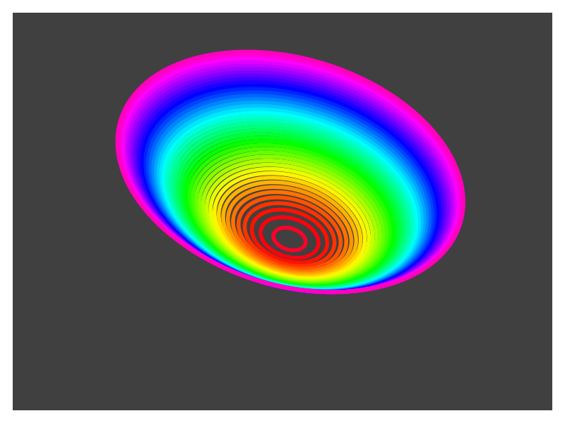
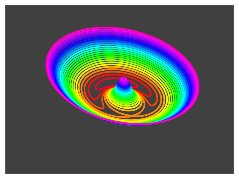
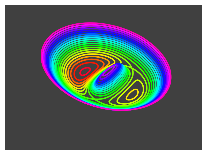
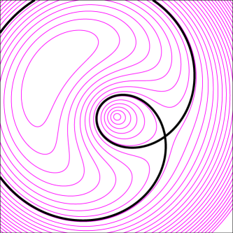
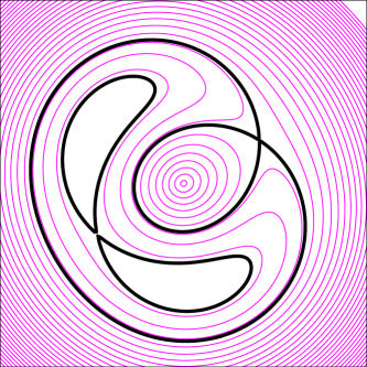
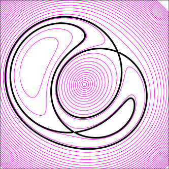
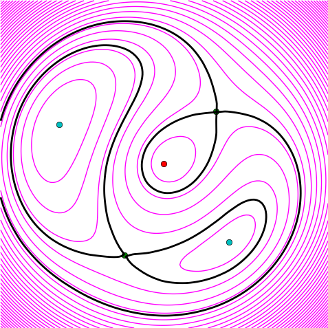
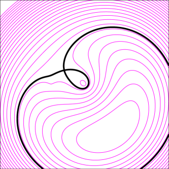
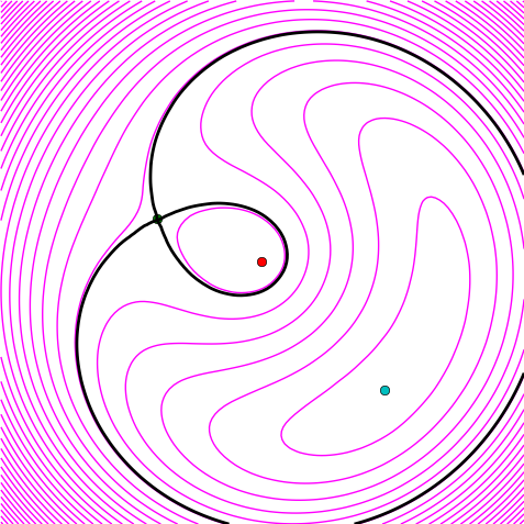
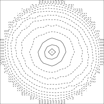
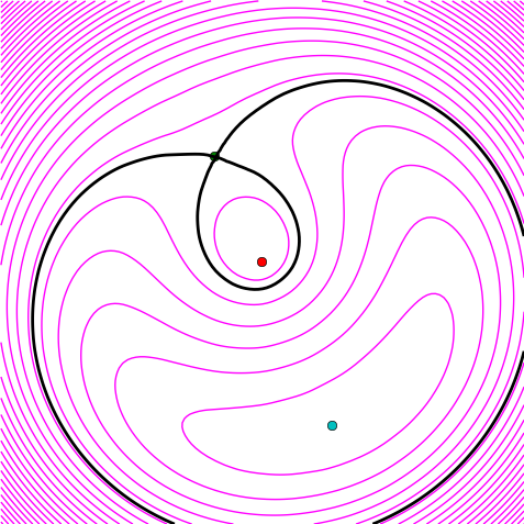
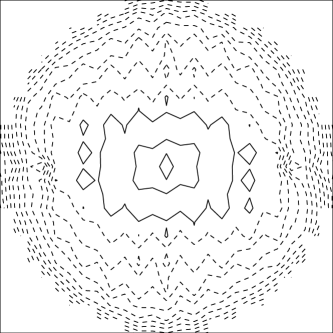
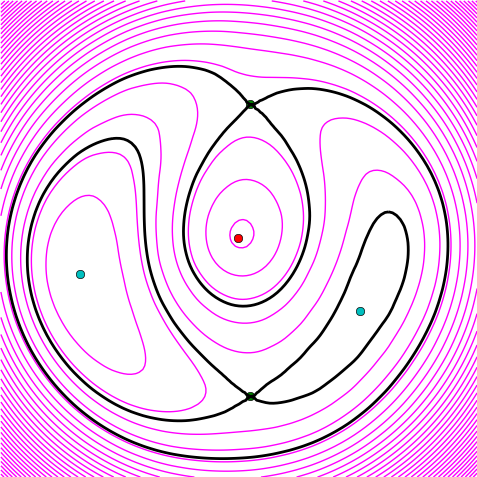
The full function $t(x,y)$, also known as the arrival-time surface, applies to virtual photons. In other words, it is an abstract construct and not itself observable. But observable image positions can be derived from the arrival-time surface, so visualising the surface is useful. Figure 1 does so. In this figure, a maximum, if present, is easy to see. To locate mimima and saddle-points, however, one needs to examine the contours of equal arrival time. A saddle point is characterised by a contour crossing itself, forming an X. Mimima, on the other hand, have contours looping around them, as do maxima.

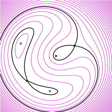
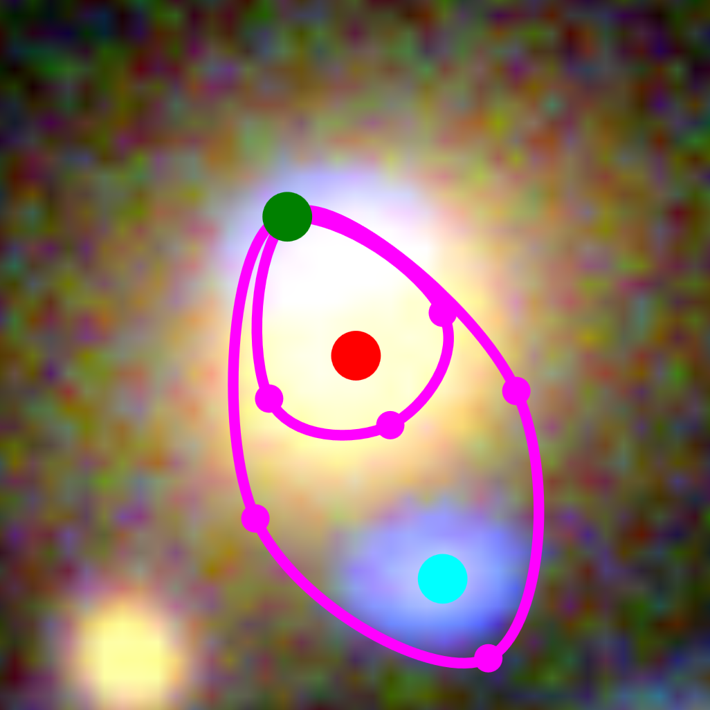
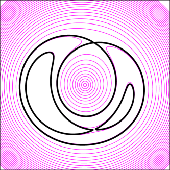
The saddle-point contours which form an X are especially interesting, because they set the overall topography of the arrival-time surface. They obviously give the locations of the saddle points, and roughly localise the minima and maxima as well. If more precise locations of the minima and maxima are added, the whole arrival-time surface is already approximately known. Since the arrival-time surface has an exact relation to the lens-mass distribution and the source position, in effect the mass distribution is also automatically approximately specified. In other words, a simple sketch of saddle-point contours along with locations of minima and maxima —which we call a “spaghetti diagram”— is implicitly already an approximation to a lens-mass distribution.

The preceding assumes a point source. To get an idea of what an extended source would do, let us imagine moving the original source slightly. The contours of constant arrival time will naturally move slightly, and so will the images. The movement of the contours will be most noticeable where the contours are far apart, that is where the arrival-time surface is nearly flat. As is evident from Figure 1, this is the region where the minimum and saddle points lie, or near the images. In this region, points on the source that are close together produce images that are comparatively far apart. In other words, the image is highly magnified. In summary, lower curvature in the arrival-time surface for a point source implies larger magnification of an extended source. Conversely, where the arrival-time surface is strongly curved, the image will be demagnified. We see from Figure 1 that the arrival-time surface tends to be highly curved near the maximum. Hence maximum tend to be demagnified. In practice, maxima of the arrival time are nearly always too faint to see. The minima and saddle points dominate.

3 A lens-modelling program

SpaghettiLens is a mass modelling program that makes use of the Space Warps infrastructure, in particular, the image database and the discussion forum. The forum is essential for establishing contact between interested members of the Space Warps community and the project science team, and then for enabling collaboration between them. We were able to collaborate together on modelling objects from Space Warps in the usual style of medium-sized astronomical collaborations, with video-conferencing and in-person meetings where possible. Preliminary results were immediately summarized on modelling threads on the forum, and anyone interested was made welcome to join at any time.

Modelling with SpaghettiLens involves three stages, (1) markup of the image, followed by (2) intensive numerical computation carried out on a server in the background, followed by (3) review of diagnostics and possible discussion. Human interaction is essential to the first and third stages, while stage 2 is completely automated. We now describe the three stages.

3.1 Image markup

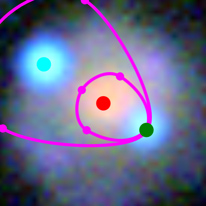
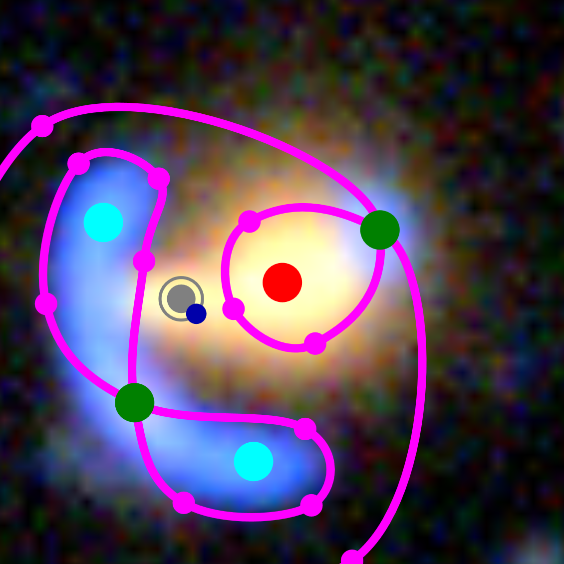
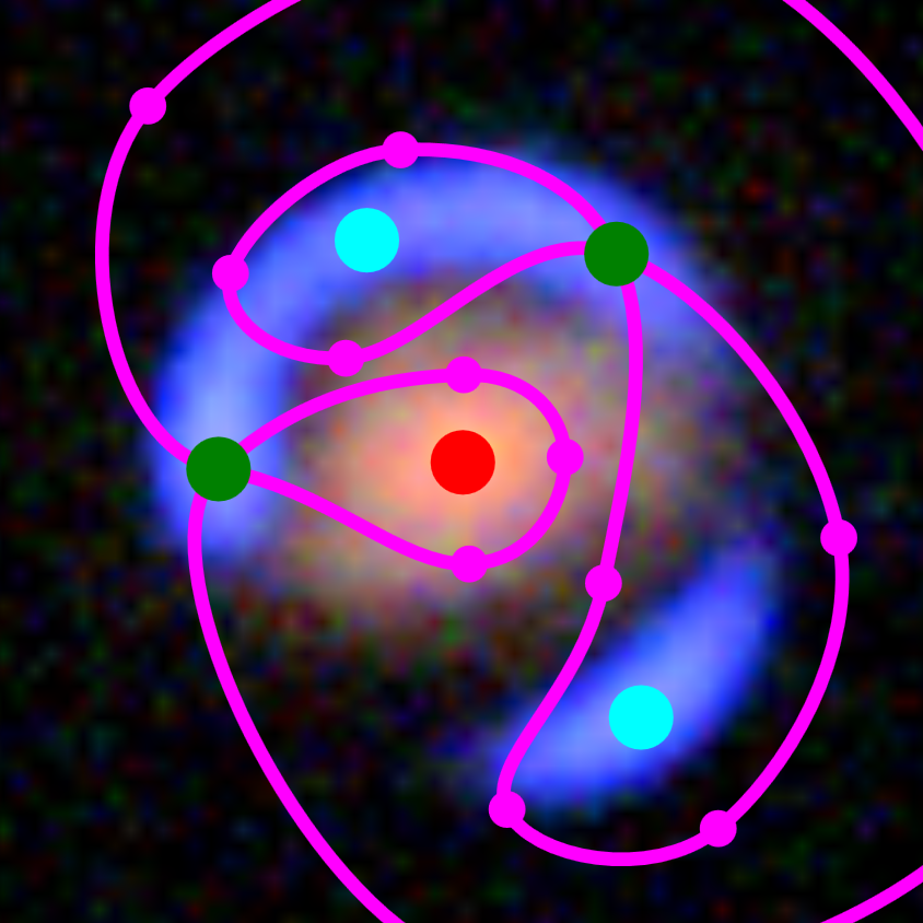
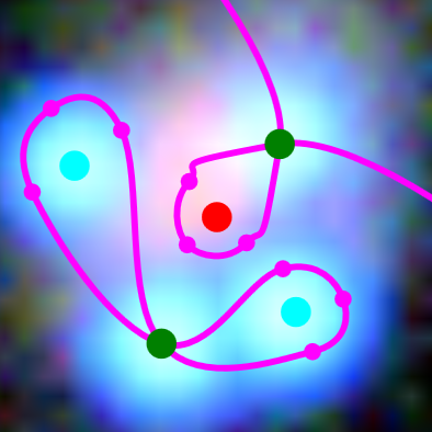
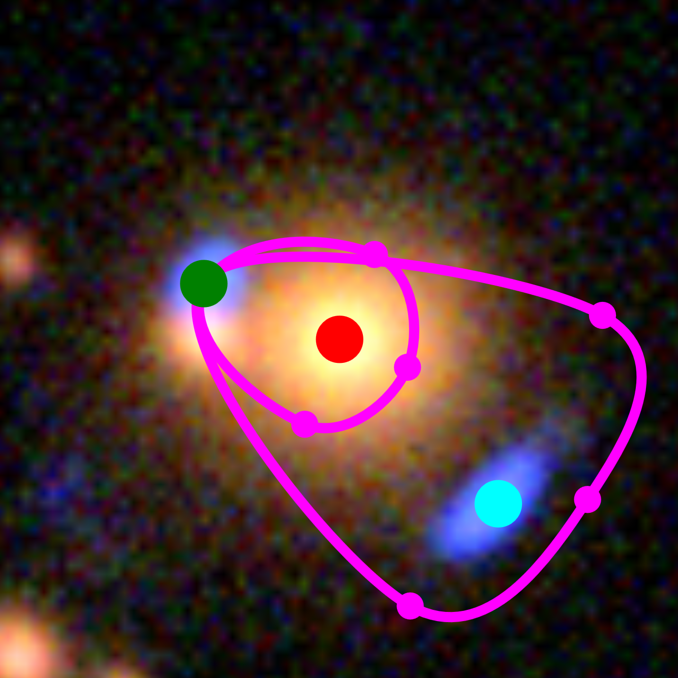
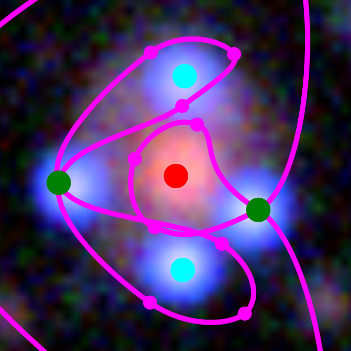
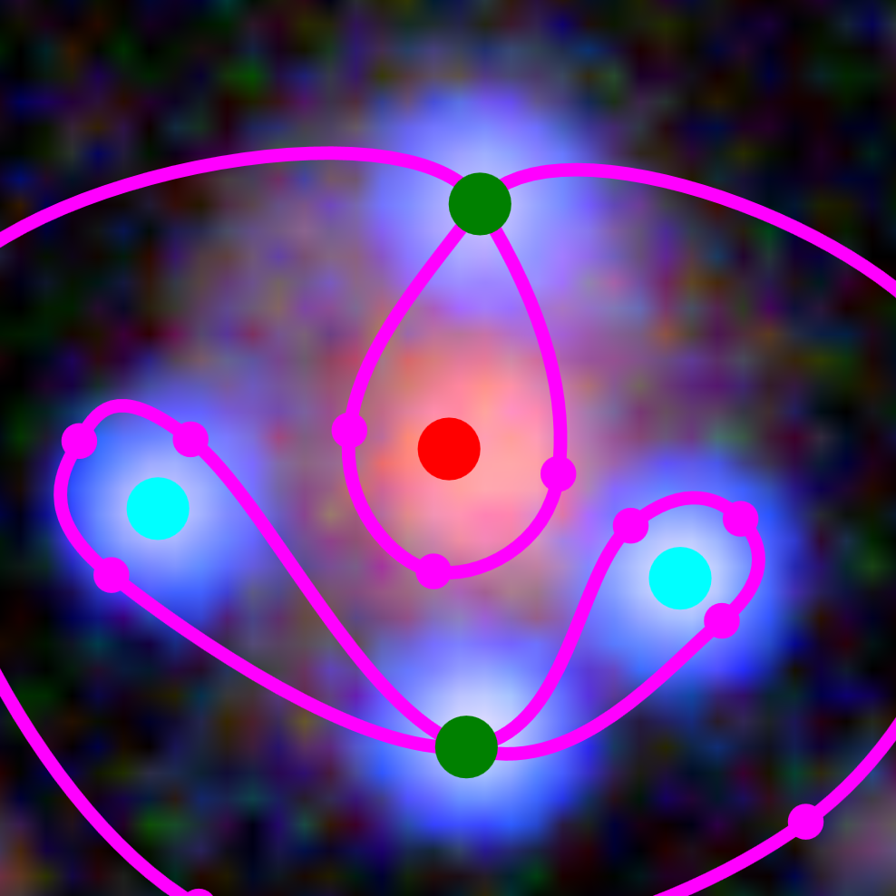
One begins by going to the SpaghettiLens web application and entering the number of a Space Warps image tile. SpaghettiLens then presents the image, along with zoom and pan options and a markup tool to construct a spaghetti diagram. The human modeller now has to make an educated guess for the topography of the arrival-time surface, and input the locations time-ordering of the maxima, minima, and saddle-points. The markup tool (which is inspired by Figure 6 of Blandford & Narayan, 1986, and is like that figure made interactive and overlaid on data) lets the modeller enter the information by sketching saddle-point contours. Examples can be seen in Figure 2 and the upper-left panels of Figures 3 to 10. The loops in the markup tool were the origin of the “spaghetti” metaphor.

Figure 2: Screen grab of SpaghettiLens in action. A Space Warps image has been loaded in, re-centred and zoomed. Five images and the associated “spaghetti” contours have then been suggested, using the marking tools associated with the buttons along the top of the panel. The mass model is generated server-side when the right-most button is pressed.

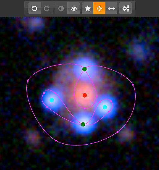
The markup tool allows only valid lensing configurations to be entered. The user does not need to think explicitly about the image parities (though the markup tool provides this information using colour codes) or about time-ordering, or worry about the odd-image theorem. The exact placement of the loops in a spaghetti diagram has no significance. Only the hierarchy of which loop is inside which is relevant. The loops are there simply to help modeller’s intuition.

As implemented so far, SpaghettiLens assumes that the lens is dominated by a single galaxy. Accordingly, only one maximum in the arrival-time surface is permitted, and it is taken to be the centre of the main lensing galaxy. The user can, however, mark additional minor galaxies: these are modelled as point masses, the mass being fitted by the program along with the rest of the mass distribution.

3.2 Numerics

Having sketched a spaghetti diagram, the user presses a button to initiate the next stage. SpaghettiLens then translates the spaghetti diagram into input for GLASS, and forwards this input. The task of GLASS, which runs server-side as it is compute-intensive, is to find a mass distribution $\kappa(x,y)$ that exactly reproduces the given locations of the maximum, minima and saddle points. This criterion by itself is extremely under-determined — there are infinitely many mass distributions that will reproduce a given set of maxima, minima and saddle points, but typically they (a) produce lots of extra images, and (b) look very unlike galaxies. Additional assumptions (a prior) are necessary. GLASS uses the following priors (cf. Saha & Williams, 1997; Coles, 2008).

1. The mass distribution is built out of non-negative tiles of mass. (Sometimes these tiles are called mass pixels, but we should emphasize that they are unrelated to image pixels, and are much larger.)

2. There is a notional lens centre, say $(x_{0},y_{0})$ which is identified with the maximum of the arrival time. The source can have an arbitrary offset with respect to the lens centre.

3. The mass distribution must be centrally concentrated, in two respects. First, the circularly averaged density must fall away like

   $$\left[(x-x_{0})^{2}+(y-y_{0})^{2}\right]^{-1/2}$$

   or more steeply. Second, the direction of increasing density at any $(x,y)$ can point at most $45^{\circ}$ away from $(x_{0},y_{0})$.

4. The lens must be symmetrical with respect to $180^{\circ}$ rotations about $(x_{0},y_{0})$. This symmetry assumption can be relaxed if the user wishes.

There are still infinitely many models that satisfy both data and prior constraints, but now they are more credible as galaxy lenses. It is then possible to generate an ensemble of models. The sampling technique used by GLASS is described in (Lubini & Coles, 2012). Typically, ensembles of 200 models are used. That is to say, what we call a SpaghettiLens model is really the mean of an ensemble of 200 models, and its estimated uncertainty is the range covered by the whole ensemble.

3.3 Diagnostics

After the model ensemble has been generated, SpaghettiLens post-processes it to present results and diagnostics to the user for inspection. This takes the form of three figures.

1. A synthetic image of the lensed features.

2. A contour map of the arrival-time surface $t(x,y)$.

3. A gray scale plus contour map of the mass distribution.

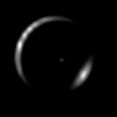
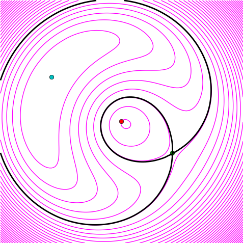
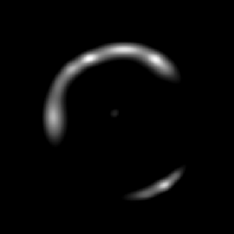
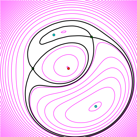
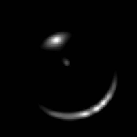
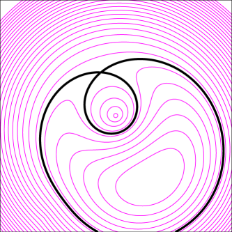
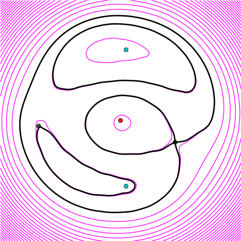
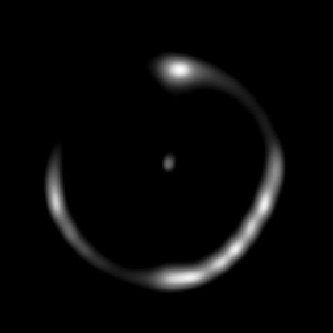
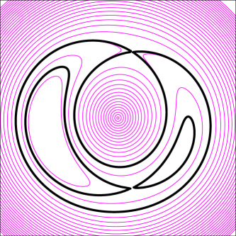
The synthetic image generated by SpaghettiLens assumes a simple circularly symmetric source with linearly decreasing surface brightness profile. The user can change the contrast level on the image, which (though it is not saved) amounts to adjusting the size of the source. These synthetic images are still very crude, and not always useful for assessing models. The best indicator, in practice, of whether the modelling was successful is contour map of $t(x,y)$, with saddle-point contours highlighted. It is, in effect, the computer’s refinement of the spaghetti diagram input by the user. If the arrival-time surface looks qualitatively similar to the spaghetti diagram, that generally indicates a successful model. The mass distribution also provides indications; successful models generally lead to smooth-looking mass distribution, whereas an irregular or checkboard pattern in the mass map signals a bad model.

After examining this feedback, the user can choose to save the model to the SpaghettiLens archive, at which point it is assigned an unique URL. They can also modify the input and try again, or discard the attempt altogether. After archiving, there can be discussion among modellers, through the Space Warps forum or by any other means, and revision of the model. This is achieved simply by sharing the model’s URL; following its hyperlink takes one to the SpaghettiLens app, pre-loaded with the correct data image and input spaghetti. Any archived model can be revised by any user: they can modify the spaghetti configuration slightly or drastically, or change options like the size of the mass tiles. Particularly interesting lens candidates lead to trees of models in this way. Discussion among modellers tends to prune a model tree, focusing attention on the most interesting models.

4 A lens modelling challenge

We now describe a test of the lens-modelling system, under conditions that mimic as closely as possible the modelling of real lens discoveries. The lenses to be modelled were the simulated lenses (known as “sims”) already sprinkled onto the Space Warps field. Once a small user base had grown around SpaghettiLens, a modelling challenge was announced through the Space Warps forum. The challenge set consisted of 29 sims, chosen to represent the different visual morphologies of Space Warps sims. Modellers then contributed 119 models for these sims (at least two for each sim). Models were reported on the same forum used to model real candidate lenses. Modellers were free to consult and refine each other’s models, but had no information on how the sims were generated.

Once the modelling was complete, the models were compared with the originals. There were two main tests: a check of whether the spaghetti diagrams were correct for the lens in question, and a comparison of the effective Einstein radii of the sims and the models.

4.1 The simulated lenses

The Space Warps sims are described in detail in More et al (in prep), but relevant here is that the sims were of three kinds, as follows.

1. Lensed quasars: The lens is modelled as a singular isothermal ellipsoid (SIE) and a constant external shear whereas the quasar is represented with a circular Gaussian source whose size is given by the point spread function (PSF) in each imaging band.

2. Galaxy-scale lenses: The lens model is the same as above whereas the background galaxy is modelled as an elliptical de Vaucouleurs.

3. Group-scale lenses: The lens model includes SIE models for the central galaxy and the inner group members, plus a circular NFW (Navarro et al., 1996, 1997) to represent the underlying dark matter distribution and the background galaxy model stays the same as galaxy-scale lenses.

Figure 3: A simulated lens that mimics a lensed quasar, and model results. The left panels derive from the simulation, and the right panels are SpaghettiLens output. Details of individual panels are in Section 4.2.

Figure 4: Results from a system with an arc plus a counter-image, typical of lensed galaxies. (See Section 4.2 for details.)

Figure 5: Another configuration of arc plus counter-image: an arc and counter image where the arc is closer to the lensing galaxy than the counter image. (See Section 4.2 for details.)

Figure 6: A four-image configuration typical of lensed quasars. (See Section 4.2 for details.)

Figure 7: A lens with unrecovered mass substructure. (See Section 4.2 for details.)

Figure 8: A sim with unrecovered substructure, resulting in a poor mass model. (See Section 4.2 for details.)

Figure 9: A four-image system with image parities incorrectly identified. The model is poor, but the estimated Einstein radius is not bad. (See Section 4.2 for details.)

Figure 10: The same system as in Figure 9, this time with image parities correctly identified. (See Section 4.2 for details.)

The gravlens program (Keeton, 2001b) was used. Formulas for the lenses appear in Keeton (2001a). The SIE lenses follow equations (33–35) of that work, with core radius set to zero. The NFW lens is in equations (48) and (50), while shear is the $\gamma$ term in equation (76).

The information in this section was not revealed to the main developer of SpaghettiLens (RK, who also chose the challenge set) or to the modellers (EB, CC, CM, JO, PS and JW) while modelling was in progress. That is, the modellers had no advance knowledge of what kind of parameterisation had been used to make the sims. After the modelling stage, AM released the details of the sims for post-modelling analysis. Results from the latter now follow.

4.2 Some example models

Of the 119 models proposed, we now discuss eight examples in some detail. Results from these are shown in Figures 3–10. The first four of these show the most common image morphologies, the other four explain some problem cases.

Each of Figures 3–10 figures has the following layout.

$$\begin{matrix}\hbox{marked-up CFHTLS image}\qquad&\hbox{model synthetic image}\\ t(x,y)&\hbox{model }t(x,y)\\ \kappa(x,y)&\hbox{model }\kappa(x,y)\end{matrix}$$

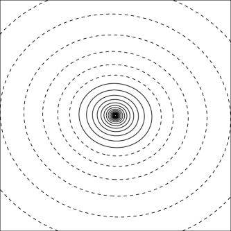
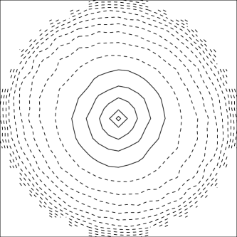
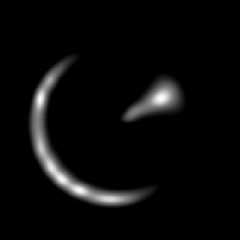
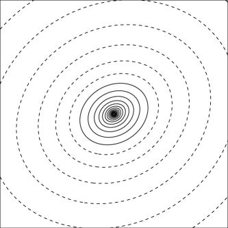
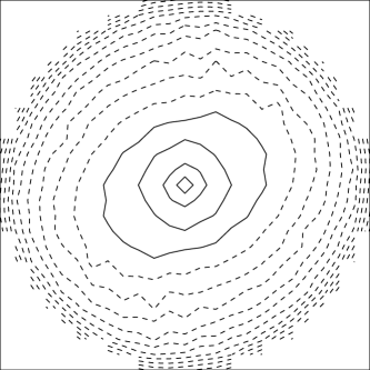
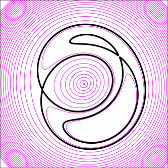
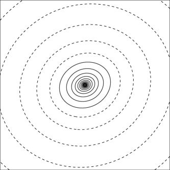
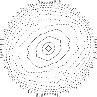
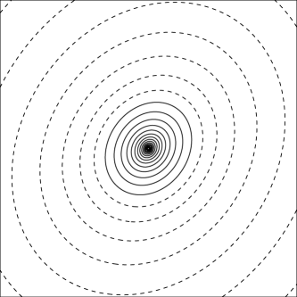
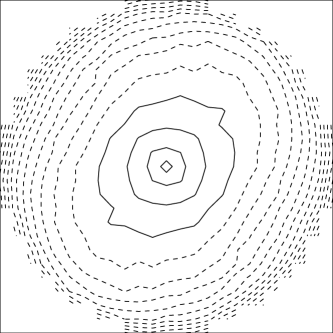
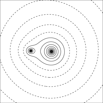
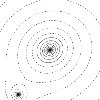
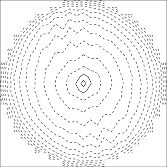
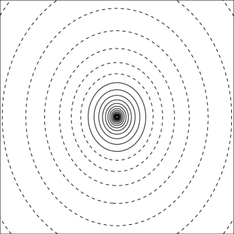
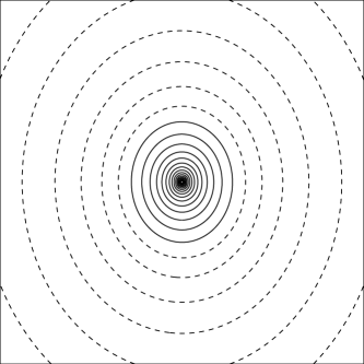
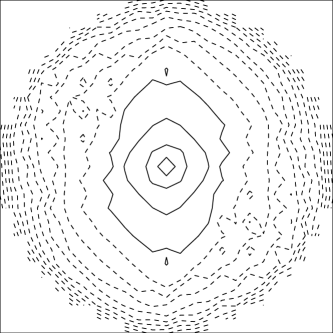
The model synthetic image presented in this paper is not the original one, but an interpolated version generated by an updated version of SpaghettiLens. The image presented during the original experiment was of lower resolution. The two plots in the middle showing $t(x,y)$ have uniform, but arbitrary spaced contour lines. The $\kappa(x,y)$ plots in the bottom row show solid lines for $\kappa>1$ and dashed lines for $\kappa<1$. The spacing is logarithmic, with 10 contours for every decade — that means contour spacing is a quarter magnitude in optical terms.

Let us now consider these cases in turn.

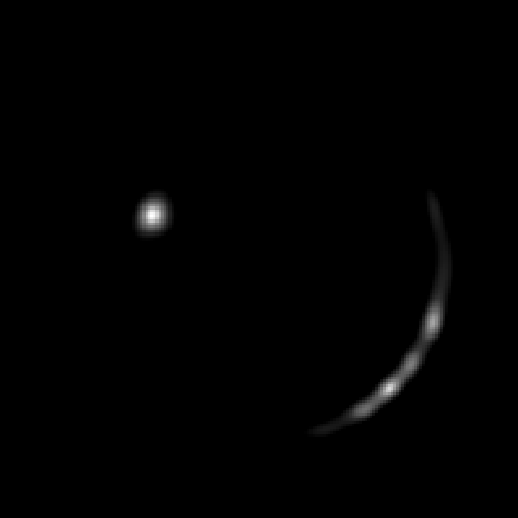
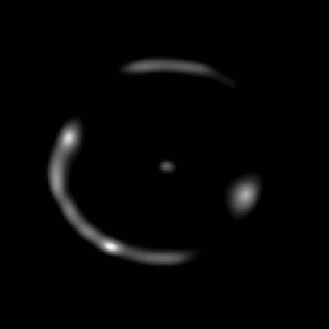
• Figure 3 shows the simplest case, with two clear images produced by a nearly-circular lens. The center of the lensing galaxy is a maximum, the image nearer to the galaxy is a saddle point, and the image further away is a minimum. All these were correctly identified. As note above, in Section 3, the precise shape of the loops in the spaghetti diagrams is unimportant, only the implied image locations, parities and time-ordering matters. $\kappa(x,y)$ shows, that the model has a more shallow mass distribution than the simulation. This is a persistent issue throughout all models and is discussed in Section 4.4.

• Figure 4 shows an example of an arc that has split into three images. This kind of configuration, with a counter-image close to the lensing galaxy and a more distant arc/triplet on the other side, generically arises from an elongated mass distribution when the source is displaced along the elongated direction. The spaghetti diagram in this case has another markup element, a grey point and circle overlaid on a probable secondary lensing galaxy. This is an instruction to SpaghettiLens to allow a point mass at that location, distinct from the main mass map.

• Figure 5 shows another example of an arc plus counter-image, but (in contrast to Figure 4) the arc is closer to the lens than the counter-image. This configuration arises if the source displacement is perpendicular to the long axis of the lensing mass. Comparing the two panels in the middle row, we see that the modeller interpreted arc as consisting of three images, whereas the sim shows a single saddle point associated with the arc. But the identification is not really erroneous — we just need to take into account that the source is extended. In fact, in the sim the brightest part of the source is only doubly imaged, but the source extends into a region that produces four images. In the $t(x,y)$ of the sim, the hairpin-bending contours are typical of double on the verge of splitting into a quad.

• Figure 6 shows another quad. This kind of configuration arises when the mass is elongated and the source is displaced at an angle to the elongation. The minima and saddle points are correctly identified, and the orientation of the ellipticity of the mass distribution is correctly reproduced.

• Figure 7 shows a lens with substructure in the form of a smaller secondary galaxy. The galaxies in such group or cluster sims were based on galaxies visible in the images, but the modelers were not told in advance whether this was the case. The minimum and saddle point are correctly identified. The mass distribution misses the substructure, but overall appears reasonable.

• Figure 8 shows a sim with substructre, like Figure 8. In comparison to the above, the resulting mass model is poor.

• Figure 9 shows a quad. In this one, the identification of the minima and saddle points was incorrect, and mass distribution comes out elongated East-West instead of North-South. The mass distribution also appears somewhat jagged and the saddle-point contours are not as clean as in the previous examples; these are often indicators of a problem with the model. The enclosed mass is, however, none the worse — the reason is probably that in a relatively symmetrical image configuration, the Einstein radius is quite well constrained by the images in a fairly model-independent way.

• Figure 10 shows another model of the same system, the only one done by an expert in this sample. The image parities are correct. The elongation has the right orientation, but is too shallow.

4.3 Test of image identification

The first post-modelling test was a qualitative comparison of the original arrival-time surfaces and the input spaghetti diagrams given by the modeller. This tested first, for correct identification and location of the lensed images, and second, for the correct parities and ordering of the lensed images in respect of the arrival time.

While we expected the identification of lensed images to be trivial, given the generally clean appearance of the sims in the test, we expected the parities and time-ordering to be more difficult. While the SpaghettiLens tutorials had provided general guidelines, to be consistently correct with the time-ordering, a modeller needs to develop some intuition for arrival time surfaces. This is an area where experience and tutorials training could improve results at a later stage, and correspondingly, feedback on the difficulties modellers encounter can help improve the tutorial materials.

Table 1 presents a summary of the test. The evaluation was done manually, comparing the input to SpaghettiLens with the actual arrival-time surface of the sim. This amounts to comparing the middle-left and middle-right panels in each of Figures 3–10, and similarly for the other 111 models.

Total	119	100%
errors in image locations	9	8%
errors in image parities or time ordering	49	41%
inaccurate image placement over an arc	21	18%
identified two images of four	5	4%
identified two nearby images as one	3	3%
missed faint images	1	1%
proposed too many images	1	1%
modelled a three-image arc as one image	4	3%
modelled one image as a three-image arc	5	4%
swapped minimum and saddle in double	2	2%
swapped minima and saddles in quad	38	32%
swapped early and late saddles in a quad	7	6%

Table 1: Table of image-identification errors and the number of models containing each. A model can contain more than one type of error.

The images of the system were considered to have been located correctly, if all the images were identified and were approximated within about 5% of SpaghettiLens frame used to draw the spaghetti diagram. That frame size is adjustable by the user, but in practice it is somewhat larger than the spaghetti diagram. Such image-placement errors were found in only 9 models. That does not include inaccurate image placement over an arc, which was considered a separate category of error.

In addition to simple image-placement errors, ten types of errors were recognised and are listed in Table 1. Most of the problems were due to unclear arc-like structures. Critical errors like the failure to identify all five images in a five images system, or to include too many images, were rare.

The assignment of the parity of the images was a more difficult task, and was successful in only about 60% of the cases. The most common error was swapping of minima and saddle-points in a quad; Figure 9 shows an example. Another, less common, error was flipping the spaghetti diagram, thus swapping the time-ordering of the two saddle points.

Incorrect image parities and time orderings tended to produce poorer-looking models, such as the checker board patterns in the mass map in Figure 9. Interestingly, however, the enclosed-mass profiles were quite robust. We will consider this aspect in the next section.

Figure 11: Mean $\kappa$ inside a circle around the lens centre, as a function of the radius of the circle. (See Section 4.4 for details.) The upper panel corresponds to the model shown in Figure 9, in which the minima and saddle-points have been incorrectly swapped. The middle corresponds to Figure 10, where the image parities were correct. The lower panel corresponds to another model, where the image parities were correct but the time-ordering was incorrect.

4.4 Test of mass-profile recovery

The second test was to compare the mass distributions $\kappa(x,y)$ of the sims and of the SpaghettiLens models. A visual comparison is presented for the eight models in Figures 3–10, in the lower-left versus lower-right panels. We will summarize the mass distributions drastically in a single number, the effective Einstein radius. Other measures for comparison of free-form lensing mass distributions appear in Coles et al. (2014), but comparing Einstein radii is already useful.

There is no standard way of defining the Einstein radius of a general non-circular lens. We adopt the simple definition

$$\langle\kappa\rangle_{\Theta_{\rm E}}=1,$$ (6)

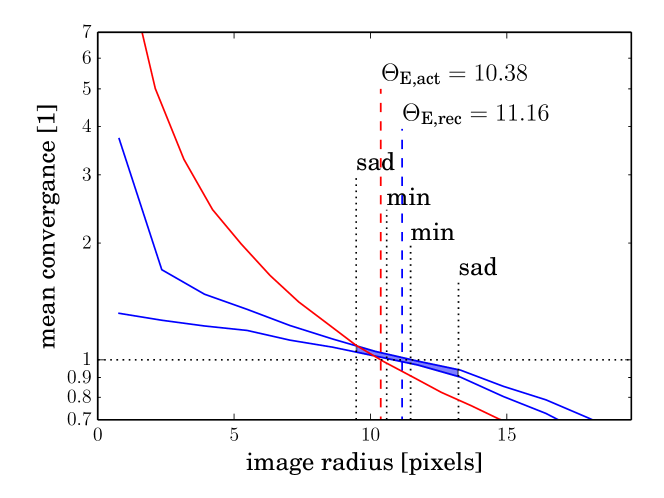
that is, the effective Einstein radius $\Theta_{\text{E}}$ is such that the mean $\kappa$ is unity inside a circle of radius $\Theta_{\text{E}}$ centered at the lens center.

Figure 12: Model-recovered versus actual Einstein radii $\Theta_{\text{E,rec}}$ and $\Theta_{\text{E,act}}$. Plus signs indicate models flagged by the modeller as failures by commenting negatively about it in the forum. Light and dark grey bands show standard deviation of volunteers (15%) and expert (10%).

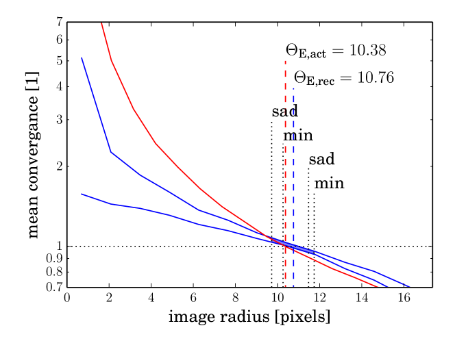
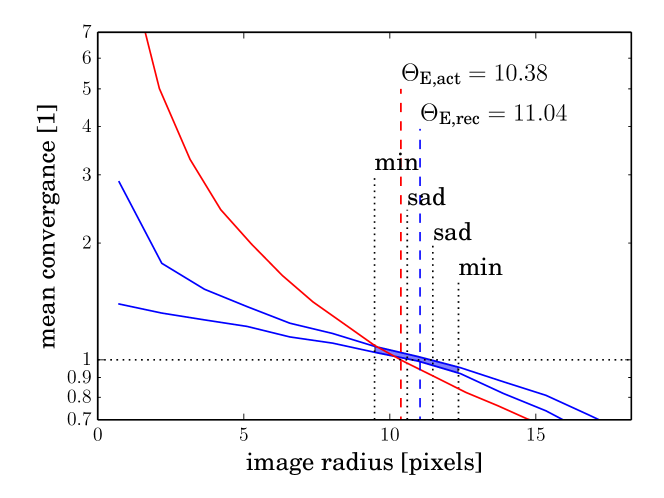
To illustrate, Figure 11 compares the circularly averaged mass profiles of three different models of one particular lens; two of the models are shown in Figures 9 and 10. Each panel in Figure 11 shows the mean $\kappa$ within a circle of given radius. The red curve is the correct profile for the sim. The two blue curves are the minimal and maximal mean enclosed $\kappa$ from the internal ensemble in SpaghettiLens. Radial locations of the images are marked, along with the image parities. The region between the blue curves is shaded between the radii of the innermost and the outermost images: this is the confidence region from the modelling. The definition (6) for $\Theta_{\text{E}}$ corresponds to crossing the dashed horizontal line at $1$: the red curve crosses the dashed line at the actual Einstein radius $\Theta_{\text{E,act}}$; the recovered Einstein radius $\Theta_{\text{E,rec}}$ and its uncertainty are given by the blue curves crossing the dashed line. We see that in all three panels, the blue curves are shallower than the red curve and $\Theta_{\text{E,rec}}$ is more than $\Theta_{\text{E,act}}$, by more than the model uncertainties. Now, steeper mass profiles tend to give wider image separations — recall that the image separation for a circular isothermal lens is 2$\Theta_{\text{E}}$, whereas for a point mass it is more (see, e.g., Courbin et al., 2002) — so $\Theta_{\text{E,rec}}$ being too high is really a consequence of the GLASS models being too shallow for the sims.

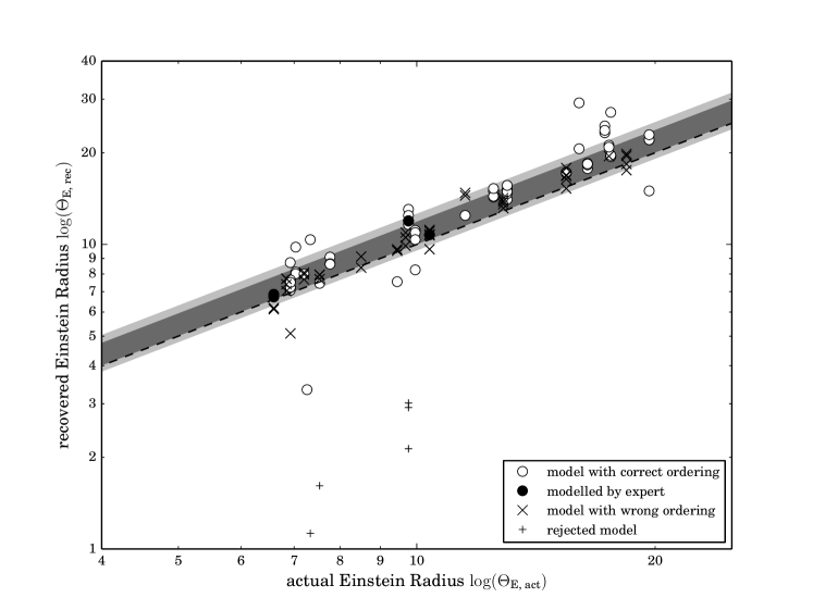
Figure 12 shows that $\Theta_{\text{E,rec}}$ of the models tend to be too high. However, this is entirely due to the GLASS model density profiles being too shallow, as illustrated above. We can separate out the performance of the SpaghettiLens interface and its users by comparing their results with the Einstein radii of SpaghettiLens models made by an expert (PS). Discounting the models which were flagged by the volunteers as poor, the mean Einstein radius overestimate was 10%, with a 15% standard deviation (shown by the light grey band in Figure 12). The expert models show a similar bias, with standard deviation 10% (the dark grey band in Figure 12). One source of this systematic error is that it is difficult to centre the lens accurately: an offset leads to a flatter mass profile for the model compared to the simulation.

5 Outlook

This work has developed the concept of saddle-point contours in the travel time of virtual photons, originally introduced by Blandford & Narayan (1986) for understanding image structure in strong gravitational lenses, into a technique for mass-mapping lenses. Despite being highly abstract, saddle-point contours look like schematic arcs, and hence lend themselves to an intuitive markup tool for lenses or lens candidates, which we call a spaghetti diagram. At the same time, saddle-point contours encode information about possible mass distributions, which can be translated into input for an existing lens-modelling engine (GLASS, by Coles et al., 2014).

SpaghettiLens is an implementation of these ideas, enabling experienced but non-professional lens enthusiasts to model newly-discovered lens candidates from the Space Warps citizen-science platform. The tests in this paper indicate that such modelling would be both feasible and scientifically interesting: given a suitable modelling tool, and appropriate guidance, a small team of non-professional volunteers was able to model a sample of 29 test lenses, and measure their Einstein radii with comparable accuracy to a professional expert.

There is, however, plenty of room for improvement:

1. SpaghettiLens tends to overestimate the Einstein radius (evident from Figure 12), and the model density profiles tend to be shallower than the SIE model used for generating the sims. The likely explanation is that while the sims are steeply peaked at the centre, the pixellated mass model fixes a comparatively large area near the central at constant density. Allowing smaller pixels in the centre region, thus enabling a steeper centre (similar to the “high resolution” feature implemented in Coles et al., 2014) may remove this bias. The use of simply parameterised, appropriately steeply-profiled models would also avoid the problem.

2. Currently, SpaghettiLens does not attempt to model the source shape; the user identifies the brightest points on the image, and these are taken as images of a point-like source, whose positions must be reproduced exactly. For generating a synthetic image, a conical source profile is assumed. Fitting for the source profile to optimize resemblance to the observed lensed image after the lens model has been generated, is algorithmically straightforward (cf. Warren & Dye, 2003; Suyu et al., 2006) and planned to be implemented. This would alleviate another problem with SpaghettiLens, which is that there is as yet no quantitative figure of merit for any given model: assessment of each model is a judgment call based on the synthetic image, and on whether the mass distribution and the arrival-time surface show suspicious features. Another possibility would be use the SpaghettiLens models as a feeder to a different lens-modelling program that already implements source-profile fitting.

3. Another limitation so far in SpaghettiLens is that the lens is assumed to be dominated by one galaxy, which puts most galaxy-group lenses beyond the reach of the modeler. Since complicated group lenses are some of the most interesting candidates present, removing this limitation is most desirable. From the users’ point of view, it would mean that spaghetti contours with more than one maximum can be allowed. For examples, see Fig. 5c in (Rusin et al., 2001) and Fig. 4b in Keeton & Winn (2003).

4. At present, a single false-color composite is used as the data. An option could be added to use all available filters, individually or in combination, at the user wishes.

5. As mentioned above, the option of revising an already-archived model is already available. Desired now are tools for comparing different models of a given system, both visually and through different statistical measures. As evidenced by a current collaborative modelling effort, a particularly interesting candidate can lead to an extended discussion and dozens of models, that in some way sample the high likelihood region of model parameter space.

6. Better tutorial materials are also needed, and this would address some of the problem areas found in the modelling challenge. For example, we saw in Section 4.3 that volunteers are most prone to making errors in two situations: when in identifying an arc- like structure while placing the points, and in identifying the correct ordering of the points in nearly-symmetric configurations. Better and more detailed introductory materials would also allow the community of modellers to grow faster and without individual instructions by experts or experienced volunteers.

The SpaghettiLens program was developed by Küng, with design suggestions from Coles, Cornen and Saha, and feedback from all co-authors. The simulations were created by A. More, in consultation with Marshall, S. More and Verma. Modelling was done by Baeten, Cornen, Macmillan, Odermatt, Saha and Wilcox, with post-modelling analysis by Küng and Saha. All authors participated in writing and editing the manuscript.

Appendix A Relation to standard lensing formalism

The description of the arrival-time surface in Sections 2 and 2.2 omitted some details for the sake of a more intuitive explanation. The convergence $\kappa$ and the geometric time delay $t_{\rm geom}$ were left as proportionalities (equations 2 and 3), and the gravitational time delay $t_{\rm grav}$ was given in an implicit form (equation 4). Here we fill in the details.

The original formulation of the arrival-time surface appears in equations (2.1) to (2.6) of Blandford & Narayan (1986). Their equations can be rearranged as follows.

$$t_{\rm geom} =\frac{(1+z_{L})}{2c}\frac{d_{S}}{d_{L}d_{LS}}\left[(x-x_{s})^{2}+(y-y_{s})^{2}\right]$$ (7)

$$\nabla^{2}t_{\rm grav} =-(1+z_{L})\frac{8\pi G}{c^{3}}\,\Sigma(x,y)$$

$$\kappa(x,y) =\frac{4\pi G}{c^{2}}\frac{d_{L}d_{LS}}{d_{S}}\times\Sigma(x,y)$$

The symbols $d_{L},d_{S}$ and $d_{LS}$ are angular-diameter distances, respectively from observer to lens, observer to source, and lens to source. We have replaced angular positions on the sky with positions on the lens plane as

$$(x,y)=d_{L}(\theta_{x},\theta_{y})\,.$$ (8)

In the concordance cosmology

$$d_{LS}=\frac{c}{H_{0}}\,\frac{1}{1+z_{S}}\,\int_{z_{L}}^{z_{S}}\!\!\frac{dz}{\sqrt{\Omega_{m}(1+z)^{3}+\Omega_{\Lambda}}}$$ (9)

and similarly $d_{L}$ and $d_{S}$.

The first line of equation (7) is $t_{\rm geom}$ from equation (3) with the proportionality filled in, and with the source offset at $(x_{s},y_{s})$ rather than at the origin.

The last line of equation (7) fills in the proportionality factor in equation (2) for the convergence (or dimensionless surface density) $\kappa$.

The middle line of equation (7) is a Poisson equation for the gravitational time delay, and is equivalent to the implicit expression (4). One way to verify the equivalence is to consider the small circle in equation (4) as a region where $\Sigma$ is constant, and approximate $t_{\rm grav}$ by its Taylor expansion to $O(x^{2},y^{2})$. Substituting in equations (7) gives the Taylor coefficients in terms of $\Sigma$, and result satisfies the expression (4). Alternatively, we can proceed with a discrete form of the Poission equation from (7). Discretising on a grid with spacing $\Delta$, we have

$$t_{\rm grav}(x,y) =\frac{1}{4}\Big{[}t_{\rm grav}(x+\Delta,y)+t_{\rm grav}(x-\Delta,y)+{}$$ (10)

$$\kern 24.0ptt_{\rm grav}(x,y+\Delta)+t_{\rm grav}(x,y-\Delta)\Big{]}$$

$$+(1+z_{L})\frac{2G}{c^{3}}\,\pi\Delta^{2}\,\Sigma(x,y)\,.$$

This is recognisable as a formula for solving the two-dimensional Poisson equation from (7) by relaxation. Let us now replace the average over four neighbouring points by the circular average $\left\langle t_{\rm grav}(x_{\lower 0.99458pt\hbox{$\circ$}},y_{\lower 0.99458pt\hbox{$\circ$}})\right\rangle$ and replace $\pi\Delta^{2}\,\Sigma(x,y)$ by the enclosed mass $M(x_{\lower 0.99458pt\hbox{$\bullet$}},y_{\lower 0.99458pt\hbox{$\bullet$}})$. These replacements are valid in the limit of a small grid. The result is the implicit equation (4).

References

- Blandford & Narayan (1986) Blandford R., Narayan R., 1986, ApJ, 310, 568
- Coles (2008) Coles J., 2008, ApJ, 679, 17
- Coles et al. (2014) Coles J. P., Read J. I., Saha P., 2014, ArXiv:1401.7990
- Courbin et al. (2002) Courbin F., Saha P., Schechter P. L., 2002, in Lecture Notes in Physics, Berlin Springer Verlag, Vol. 608, Gravitational Lensing: An Astrophysical Tool, Courbin F., Minniti D., eds., p. 1
- Gavazzi et al. (2014) Gavazzi R., Marshall P. J., Treu T., Sonnenfeld A., 2014, ApJ, 785, 144
- Keeton (2001a) Keeton C. R., 2001a, ArXiv: astro-ph/0102341
- Keeton (2001b) Keeton C. R., 2001b, ArXiv: astro-ph/0102340
- Keeton & Winn (2003) Keeton C. R., Winn J. N., 2003, ApJ, 590, 39
- Khatib et al. (2011) Khatib F., Cooper S., Tyka M. D., Xu K., Makedon I., Popović Z., Baker D., Players F., 2011, Proceedings of the National Academy of Sciences, 108, 18949
- Koopmans et al. (2009) Koopmans L. V. E. et al., 2009, ApJL, 703, L51
- Lefor (2014) Lefor A. T., 2014, Astronomy and Computing, 5, 28
- Leier et al. (2011) Leier D., Ferreras I., Saha P., Falco E. E., 2011, ApJ, 740, 97
- Lubini & Coles (2012) Lubini M., Coles J., 2012, MNRAS, 425, 3077
- Marshall et al. (2009) Marshall P. J., Hogg D. W., Moustakas L. A., Fassnacht C. D., Bradač M., Schrabback T., Blandford R. D., 2009, ApJ, 694, 924
- Marshall et al. (2005) Marshall P. J., Moustakas L. A., Hogg D. W., Bradac M., Fassnacht C. D., Blandford R. D., 2005, in Bulletin of the American Astronomical Society, Vol. 37, American Astronomical Society Meeting Abstracts, p. #200.03
- More et al. (2012) More A., Cabanac R., More S., Alard C., Limousin M., Kneib J.-P., Gavazzi R., Motta V., 2012, ApJ, 749, 38
- Naudus et al. (2010) Naudus P., Wallin J., Marshall P., 2010, in Bulletin of the American Astronomical Society, Vol. 42, American Astronomical Society Meeting Abstracts #215, p. 435.27
- Navarro et al. (1996) Navarro J. F., Frenk C. S., White S. D. M., 1996, ApJ, 462, 563
- Navarro et al. (1997) Navarro J. F., Frenk C. S., White S. D. M., 1997, ApJ, 490, 493
- Oguri & Marshall (2010) Oguri M., Marshall P. J., 2010, MNRAS, 405, 2579
- Raddick et al. (2013) Raddick M. J. et al., 2013, Astronomy Education Review, 12, 010106
- Refsdal (1964) Refsdal S., 1964, MNRAS, 128, 307
- Refsdal (1966) Refsdal S., 1966, MNRAS, 132, 101
- Rusin et al. (2001) Rusin D. et al., 2001, ApJ, 557, 594
- Saha & Williams (1997) Saha P., Williams L. L. R., 1997, MNRAS, 292, 148
- Schwamb et al. (2013) Schwamb M. E. et al., 2013, ApJ, 768, 127
- Sereno & Paraficz (2014) Sereno M., Paraficz D., 2014, MNRAS, 437, 600
- Suyu et al. (2006) Suyu S. H., Marshall P. J., Hobson M. P., Blandford R. D., 2006, MNRAS, 371, 983
- Walsh et al. (1979) Walsh D., Carswell R. F., Weymann R. J., 1979, Nature, 279, 381
- Warren & Dye (2003) Warren S. J., Dye S., 2003, ApJ, 590, 673
- Weymann et al. (1980) Weymann R. J. et al., 1980, Nature, 285, 641
- Young et al. (1981a) Young P., Deverill R. S., Gunn J. E., Westphal J. A., Kristian J., 1981a, ApJ, 244, 723
- Young et al. (1981b) Young P., Gunn J. E., Oke J. B., Westphal J. A., Kristian J., 1981b, ApJ, 244, 736
- Zwicky (1937) Zwicky F., 1937, ApJ, 86, 217